Density profiles near nuclear surface of ^44,52Ti: An indication of $\alpha$ clustering

Abstract

We investigate the degree of $\alpha$ (⁴He nucleus) clustering in the ground-state density profiles of ⁴⁴Ti and ⁵²Ti. Two types of density distributions, shell- and cluster-model configurations, are generated fully microscopically with the antisymmetrized quasi-cluster model, which can describe both the $j$-$j$ coupling shell and $\alpha$-cluster configurations in a single scheme. Despite both the models reproducing measured charge radius data, we found that the $\alpha$ clustering significantly diffuses the density profiles near the nuclear surface compared to the ideal $j$-$j$ coupling shell model configuration. The effect is most significant for ⁴⁴Ti, while it is less for ⁵²Ti due to the occupation of the $0f_{7/2}$ orbits in the ⁴⁸Ca core. This difference can be detected by measuring proton-nucleus elastic scattering or the total reaction cross section on a carbon target at intermediate energies.

I Introduction

Nucleon density distributions include various information on the nuclear structure. Saturation of the nuclear density in the internal region and the drop off at the nuclear surface were revealed by systematic measurements of charge density distributions using electron scattering [1]. The nucleon density distribution can also be obtained using proton-nucleus elastic scattering [2]. Such measurements were extended to unstable nuclei using the inverse kinematics [3]. Since the nuclear density is saturated in the internal region, the nuclear structure information is obtained near the nuclear surface [4, 5]. For example, nuclear deformation induces a sudden enhancement of the nuclear matter radius [8, 9, 10, 11, 6, 7, 12, 13, 14], where the density profile near the nuclear surface is significantly diffused compared to the spherical configuration [15, 16]. The nuclear “bubble” structure, the internal density depression can also be imprinted on the nuclear surface [17].

We explore how the nuclear structure affects the density profiles near the nuclear surface. These days, exploring an $\alpha$ (⁴He nucleus) cluster in medium to heavy mass nuclei has attracted attention in the context of the astrophysical interest [18]. Direct measurement of the degree of $\alpha$ clustering near the nuclear surface has been realized using $\alpha$ knockout reactions [19]. The quantification of the degree of $\alpha$ clustering may impact the determination of the reaction rates of astrophysically important reactions involving medium mass nuclei.

Although the clustering is exotic and intriguing to explore, the standard picture for the nuclear structure is shell structure, and the difference between these two must appear in the density profiles near the nuclear surface. Here we choose ⁴⁴Ti and ⁵²Ti as representatives of medium mass nuclei. The well-developed ${}^{40}{\rm Ca}+\alpha$ structure of ⁴⁴Ti was predicted in Ref. [20]. Afterward, the inversion doublet structure was confirmed experimentally [21, 22] as its supporting evidence. The $\alpha$-cluster structure of ⁴⁴Ti was microscopically investigated [23]. Establishing the degree of the clustering in ⁴⁴Ti may impact ${}^{40}{\rm Ca}(\alpha,\gamma)^{44}{\rm Ti}$ reaction rate [24]. The influence of the $\alpha$ clustering on the reaction rate was discussed for ⁴⁸Ti using the $(p,p\alpha)$ knockout reactions [25]. We remark that the mechanism of the emergence of the $\alpha$ cluster near the nuclear surface in medium mass nuclei is recently suggested concerning the tensor force [26].

In this paper, we discuss the difference of the density profiles near the nuclear surface between cluster and shell models by taking an example of ⁴⁴Ti. We also examine the case of ⁵²Ti to clarify the role of excess neutrons. The study along this line may give a hint for the research for the emergent mechanism of $\alpha$ particle in the neutron-rich nuclei toward understanding nuclear matter properties. For this purpose, we need a model that can describe both the shell and cluster configurations in a single scheme. Here we employ the antisymmetrized quasi-cluster model (AQCM [27, 28, 29, 30, 31, 32, 33, 34, 35, 36, 37, 38, 39, 40]). This model allows to smoothly transform the cluster model wave function to the $j$-$j$ coupling shell one and these two can be treated on the same footing.

The paper is organized as follows. Section II summarizes the present approach to investigate the $\alpha$ clustering in the density profiles of ⁴⁴Ti and ⁵²Ti. How to calculate the density distributions that have shell and cluster configurations using the AQCM is explained in Sec. II.1. For the sake of convenience, some definitions of the nuclear radii are given in Sec. II.2. To connect obtained density profiles with reaction observables, a high-energy reaction theory, the Glauber model is briefly explained in Sec. II.3. Section III presents our results. First, in Sec. III.1, we discuss the properties of the wave functions with the shell and cluster configurations. Definitions and characteristics of the two types of model wave functions are described in detail. In Sec. III.2, we compare the resulting density profiles and discuss the relationship between these density profiles and reaction observables. Section III.3 clarifies the difference in the shell- and cluster-model approaches in the density profiles. Finally, the conclusion is given in Sec. IV.

II Methods

II.1 Density distribution with antisymmetrized quasi-cluster model (AQCM)

The AQCM ansatz of the core (⁴⁰Ca or ⁴⁸Ca) plus $\alpha$ particle wave function, which can be transformed to $j$-$j$ coupling shell model one, is defined by fully antisymmetric $(\mathcal{A})$ product of the core and $\alpha$ wave functions as

$$\Phi(\nu_{\rm C},\nu_{\alpha},R,\Lambda_{p},\Lambda_{n})=\mathcal{A}\left\{\Phi_{\rm C}(\nu_{\rm C})\Phi_{\alpha}(\nu_{\alpha},R,\Lambda_{p},\Lambda_{n})\right\}.$$ (1)

The wave function of the core nucleus $\Phi_{C}$ with the oscillator size parameter $\nu_{C}$ is constructed based on the multi-$\alpha$ cluster model [41]. For ⁴⁰Ca, the core wave function is obtained by taking small distances among ten $\alpha$ clusters; this nucleus corresponds to the closure of the $sd$-shell and the shell- and cluster-model wave functions coincide at the zero-distance limit of the inter-cluster distances. For ⁴⁸Ca, we need to put additional eight neutrons describing the neutron number $N=28$, subclosure of the $0f_{7/2}$ shell, and AQCM allows a simple description to transform the cluster model. The details are given in Ref. [32].

The wave function of the $\alpha$ particle at the distance between the center-of-mass coordinate of the core and $\alpha$ particles, $R$, is defined as the product of the single-particle Gaussian wave packet as

$$\Phi_{\alpha}(\nu,R,\Lambda_{p},\Lambda_{n})=\phi^{\nu}_{1}(\uparrow,p)\phi^{\nu}_{2}(\downarrow,p)\phi^{\nu}_{3}(\uparrow,n)\phi^{\nu}_{4}(\downarrow,n)$$ (2)

with a single-nucleon Gaussian wave packet with spin $\chi_{s}$ ($s=\uparrow$ or $\downarrow$) and isospin $\eta_{t}$ ($t=p$ or $n$) wave functions

$$\phi^{\nu}_{i}(s,t)=\left(\frac{2\nu}{\pi}\right)^{3/4}\exp\left[-\nu(\bm{r}_{i}-\bm{\zeta}_{t})^{2}\right]\chi_{s}\eta_{t},$$ (3)

where

$$\bm{\zeta}_{t}=\bm{R}+i\Lambda_{t}\bm{e}_{t}^{\rm spin}\times\bm{R}$$ (4)

with $\bm{e}^{\rm spin}_{t}$ being a unit vector for the intrinsic-spin orientation of a nucleon. Note that it corresponds to the ordinary Brink $\alpha$-cluster wave function in Ref. [41] by taking $\Lambda_{t}=0$. A limit of $R\to 0$ leads to the SU(3) limit of the shell model configuration. The $j$-$j$ coupling shell model wave function can be expressed by introducing $\Lambda_{t}=1$ with $R\to 0$ [30]. For example, in ⁴⁴Ti, the $\alpha$ cluster is changed into $(0f_{7/2})^{4}$ configuration using AQCM. Thus, the model wave function can describe both the shell and $\alpha$-cluster configurations in a single scheme.

Finally, the density distribution in the laboratory frame is obtained by averaging the intrinsic density distribution over angles as

$$\rho_{t}(r)=\frac{1}{4\pi}\,\int d\hat{\bm{r}}\,\rho^{\rm int}_{t}(\bm{r}),$$ (5)

where $\rho^{\rm int}_{t}$ is obtained by using the Slater determinant of ⁴⁴Ti or ⁵²Ti represented as $\Phi$

$$\rho^{\rm int}_{t}(\bm{r})=\langle\Phi|\sum_{i\in t}\delta(\bm{r}_{i}-\bm{r})|\Phi\rangle/\langle\Phi|\Phi\rangle,$$ (6)

where the summation is taken over protons ($t=p$) or neutrons ($t=n$). Note that $\sum_{i=1}^{A}\left<\bm{r}_{i}\right>=0$ is imposed and the center-of-mass motion is ignored as the mass number $A\approx 40$–50 is large.

II.2 Definitions of radii

The root-mean-square (rms) point-proton, neutron, and matter radii are calculated by

$$r_{p} =\sqrt{\frac{4\pi}{Z}\int_{0}^{\infty}dr\,r^{4}\rho_{p}(r)},$$ (7)

$$r_{n} =\sqrt{\frac{4\pi}{N}\int_{0}^{\infty}dr\,r^{4}\rho_{n}(r)},$$ (8)

$$r_{m} =\sqrt{\frac{4\pi}{A}\int_{0}^{\infty}dr\,r^{4}[\rho_{p}(r)+\rho_{n}(r)]},$$ (9)

where $Z$ denotes the proton number. The charge radius $r_{\rm ch}$ is converted from the theoretical point-proton radius $r_{p}$ by using the formula [42, 43]

$$r_{\rm ch}^{2}=r_{p}^{2}+r_{{\rm ch},p}^{2}+\frac{N}{Z}r^{2}_{{\rm ch},n}+\frac{3\hbar^{2}}{4m_{p}^{2}c^{2}}.$$ (10)

where $r^{2}_{{\rm ch},t}$ is the second moment of the nucleon charge distribution, and the fourth term of Eq. (10) is the so-called Darwin-Foldy term, which comes from relativistic correction.

II.3 Reaction observables within the Glauber model

Proton-nucleus elastic scattering at intermediate energy is one of the most direct ways to extract the density profiles near the nuclear surface. We remark that the whole density distribution can be obtained by measuring up to backward angles [44, 45], although the internal density has large uncertainties. As long as the nuclear surface density is of interest, only the cross sections at the forward angles, to be more specific, the cross section at the first peak in proton-nucleus diffraction is needed to extract the “diffuseness” of the density distribution as prescribed in Ref. [15]. To connect the density profile with observables at intermediate energies, we employ a high-energy microscopic reaction theory, the Glauber model [46].

The elastic scattering differential cross section is evaluated by

$$\frac{d\sigma}{d\Omega}=|f(\theta)|^{2}$$ (11)

with the scattering amplitude of the proton-nucleus elastic scattering [47]

$$f(\theta)=F_{C}(\theta)+\frac{ik}{2\pi}\int d\bm{b}\,e^{-i\bm{q}\cdot\bm{b}+2i\eta\ln(kb)}\left(1-e^{i\chi_{pT}(\bm{b})}\right),$$ (12)

where $F_{C}(\theta)$ is the Rutherford scattering amplitude, $\bm{b}$ is the impact parameter vector, and $\eta$ is the Sommerfeld parameter. The relativistic kinematics is used for the wave number $k$.

The optical phase-shift function $\chi_{pT}$ includes all dynamical information in the Glauber model, but its evaluation involves multi-fold integrations. For practical calculations, the optical-limit approximation (OLA) [46, 47] is made to compute the optical phase-shift function as

$$i\chi_{pT}(\bm{b})\approx-\int d\bm{r}\,\left[\rho_{p}(\bm{r})\Gamma_{pp}(\bm{b}+\bm{s})+\rho_{n}(\bm{r})\Gamma_{np}(\bm{b}+\bm{s})\right],$$ (13)

where $\bm{r}=(\bm{s},z)$ with $z$ being the beam direction. The inputs to the theory are the projectile’s density distributions and proton-proton (neutron-proton) profile function $\Gamma_{pp}$ ($\Gamma_{np}$). The parameterization of the profile function is given in Ref. [48]. Once all the inputs are set, the theory has no adjustable parameter, and thus, the resulting reaction observables must reflect the density profiles of the projectile nucleus. The OLA works well for proton-nucleus scattering as demonstrated, e.g., in Refs. [49, 53], and its accuracy compared to those obtained by the full evaluation of the optical phase-shift function were discussed in Refs. [50, 51, 52, 53].

The density profile can also be reflected in the total reaction cross sections at medium to high incident energies, which are a standard physical quantity to investigate the nuclear size properties. Here, we investigate the total reaction cross sections on a carbon target as a carbon target is superior than a proton target to probe the density distributions near the nuclear surface [54, 55]. In the Glauber model [46], the cross section is calculated as

$$\sigma_{R}=\int d\bm{b}\,\left(1-|e^{i\chi_{PT}(\bm{b})}|^{2}\right).$$ (14)

Since the multiple scattering effects cannot be neglected in the nucleus-nucleus collision, the nucleon-target formalism in the Glauber model [56] is employed to evaluate projectile-target optical phase-shift function $\chi_{PT}(\bm{b})$. The inputs to the theory are the density distributions of the projectile and target and the profile function. We take harmonic-oscillator type density for the target density that reproduces the measured charge radius of ¹²C [43]. This model works well in many examples of the nucleus-nucleus scattering involving unstable nuclei [57, 58, 51, 59, 11, 13, 52] and is a standard tool to extract nuclear size properties from the interaction cross section measurements [60, 61, 62].

III Results and discussions

III.1 Properties of the wave functions

Here we examine two types of model wave functions: one is a shell-model-like configuration (S-type), and another is a cluster-model-like configuration (C-type). Both models reproduce the experimental charge radius data of ⁴⁴Ti. To clarify the role of the excess neutrons, we examine ⁵²Ti as well. Note that the charge radius of ⁵²Ti has not been measured yet, and thus we use the data of the neighboring nucleus, ⁵⁰Ti, 3.57 fm [43] as a reference. In the following two subsubsections, we explain how to construct the two model wave functions in detail.

III.1.1 Shell-model-like configuration (S-type)

The shell-model-like wave function (S-type) is practically constructed by taking the core-$\alpha$ distance $R$ small with $\nu_{C}=\nu_{\alpha}=\nu$. It is known that this limit goes to the SU(3) shell model configuration [41]. For ⁴⁴Ti, to express the $j$-$j$ coupling shell model wave function, we take $\Lambda_{p}=\Lambda_{n}=1$ [26], and thus the wave function of the valence nucleon orbit becomes $(0f_{7/2})^{2}_{p}(0f_{7/2})^{2}_{n}$, where $p$ is for proton and $n$ is for neutron. In this S-type wave function, as we fix the core-$\alpha$ distance small, we only have one parameter, the oscillator size parameter of ⁴⁴Ti, $\nu$. This is fixed to reproduce the point-proton radius extracted from the charge radius data of ⁴⁴Ti. To confirm the configurations are all right, we evaluate the total harmonic oscillator quanta $\left<Q\right>$, the expectation values of single-particle spin-orbit operators $\sum_{i=1}^{A}\bm{l}_{i}\cdot\bm{s}_{i}$, $\left<LS\right>$, and single-particle parity operators $\sum_{i=1}^{A}P_{i}$ with $P_{i}f(\bm{r}_{i})=f(-\bm{r}_{i})$, $\left<P\right>$. The last quantity represents difference of number of particles in the positive-parity orbits and negative-parity orbits. These calculated values are listed in Table 1 and perfectly agree with the results expected from ideal shell model configurations: $\left<Q\right>=60$, $\left<LS\right>=0$, and $\left<P\right>=16$ for ⁴⁰Ca with the closed $sd$ shell and 72, 6, and 12 for ⁴⁴Ti with the $(0f_{7/2})^{2}_{p}(0f_{7/2})^{2}_{n}$ configuration.

For ⁴⁸Ca, these values also agree with the ideal values of the shell model, $\left<Q\right>=84$, $\left<LS\right>=12$, and $\left<P\right>=8$. In the case of ⁵²Ti, as it differs from the case of ⁴⁴Ti, we take $\Lambda_{p}=1$ and $\Lambda_{n}=0.5$, resulting in the desired expectation values $\left<Q\right>=96$, $\left<LS\right>=16$, and $\left<P\right>=4$ for the $(0f_{7/2})^{2}_{p}(1p_{3/2})^{2}_{n}$ configuration. This is because the $0f_{7/2}$ neutron orbit is already filled by the core nucleus. The additional two neutrons are found to occupy higher $j$-upper orbits such as $0g_{9/2}$ when $\Lambda_{n}=1$. In fact, we get $\left<Q\right>\approx 98$ when $\Lambda_{p}=\Lambda_{n}=1$ is taken. As the charge radius of ⁵²Ti is unknown, we also generate the ⁵²Ti wave function by extending the point-proton radius $r_{p}$ by 0.05 fm, which is listed as “extended” S-type.

III.1.2 $\alpha$-cluster-like configuration (C-type)

Table 1: Properties of the shell-model-like (S-type) and $\alpha$-cluster-model-like (C-type) wave functions. Values in parentheses are obtained with ideal configurations.

		$\nu$ (fm-2)	$R$ (fm)	$\Lambda_{p}$	$\Lambda_{n}$	$\left<Q\right>$	$\left<LS\right>$	$\left<P\right>$	$r_{\rm ch}$ (fm)
40Ca		0.1315	–	–	–	60.0 (60)	0.0 (0)	16.0 (16)	3.478
44Ti (S-type)		0.1270	0.20	1	1	72.0 (72)	6.0 (6)	12.0 (12)	3.611
44Ti (C-type)		0.1315	2.85	0	0	72.9	0.0 (0)	13.2	3.611
48Ca		0.1311	–	–	–	84.2 (84)	12.0 (12)	8.4 (8)	3.476
52Ti (S-type)		0.1297	0.20	1	0.5	96.2 (96)	15.5 (16)	4.4 (4)	3.569
52Ti (C-type)		0.1311	1.60	0	0	96.5	11.2	4.9	3.569
52Ti (extended, S-type)		0.1260	0.20	1	0.5	96.2 (96)	15.5 (16)	4.4 (4)	3.619
52Ti (extended, C-type)		0.1311	3.01	0	0	97.4	11.4	5.9	3.619

The $\alpha$-cluster-model wave function (C-type) is constructed based on the core plus $\alpha$-cluster model. In this case, we take $\Lambda_{p}=\Lambda_{n}=0$, where the four nucleons are localized at a distance $R$ from the core nucleus. The size parameters of the core wave functions are respectively fixed to reproduce the charge radii of ^40,48Ca. For the C-type wave functions of ^44,52Ti, for the sake of simplicity, we set $\nu_{\rm C}=\nu_{\alpha}=\nu$. This is reasonable because $\alpha$-particle near the nuclear surface can be distorted by the interaction and Pauli principle from the core. In fact, the size of $\alpha$-particle is somewhat enlarged compared to that in vacuum [63]. Finally, the distances between the core and $\alpha$ particle, $R$, of ⁴⁴Ti and ⁵²Ti are respectively fixed to reproduce their charge radii. Hereafter we refer to this model as C-type.

Table 1 also lists the properties of the C-type wave functions. For ⁴⁴Ti, the $\left<LS\right>$ values are zero as $\Lambda_{p}=\Lambda_{n}=0$. The core and cluster distance is determined to be $R=2.85$ fm, implying well-developed $\alpha$ clustering near the nuclear surface. $\left<Q\right>$ is a bit larger than that of the S-type. This is due to the mixing of $sdg$-shell orbit ($\left<Q_{i}\right>=4,\left<P_{i}\right>=+1$), which can be confirmed from the fact that the $\left<P\right>$ value of the C-type is larger than that of the S-type.

For ⁵²Ti, the core-$\alpha$ distance is found to be smaller, $R=1.60$ fm to reproduce the charge radius of ⁵⁰Ti. The S-type and C-type wave functions give similar $\left<Q\right>$ values, while $\left<LS\right>$ value is reduced for the C-type wave function because $\alpha$ cluster part does not contribute to this value.

The distance becomes comparable to that of ⁴⁴Ti, $R\approx 3$ fm when the extended charge radius is assumed for ⁵²Ti. In that case, an increase of the $\left<Q\right>$ and $\left<P\right>$ values are attained by the contribution of higher shell, which is the same reason found in ⁴⁴Ti. The $\left<LS\right>$ value is also reduced for the C-type compared to the S-type by the same amount as in the case of those reproducing the charge radius of ⁵⁰Ti because the S-type wave function includes $1p_{3/2}$ orbits, while the C-type wave function has no contribution from the $\alpha$ cluster part.

III.2 Density profiles and reaction observables

Table 2: Rms point-proton, neutron, and matter radii and diffuseness parameters for proton, neutron, and matter in units of fm.

		$r_{p}$	$r_{n}$	$r_{m}$	$a_{p}$	$a_{n}$	$a_{m}$
40Ca		3.38	3.38	3.38	0.551	0.551	0.551
44Ti (S-type)		3.51	3.51	3.51	0.557	0.557	0.557
44Ti (C-type)		3.51	3.51	3.51	0.625	0.625	0.625
48Ca		3.38	3.62	3.52	0.552	0.528	0.540
52Ti (S-type)		3.48	3.68	3.59	0.552	0.574	0.572
52Ti (C-type)		3.48	3.67	3.59	0.608	0.566	0.593
52Ti (extended, S-type)		3.53	3.73	3.65	0.558	0.584	0.579
52Ti (extended, C-type)		3.53	3.71	3.63	0.630	0.579	0.606

Here we investigate the difference between these density profiles obtained in the previous section. Table 2 lists the root-mean-square (rms) point-proton $(r_{p})$, neutron $(r_{n})$, and matter ($r_{m}$) radii of these density models employed in this paper. Thus far, we have obtained different density profiles that have the same charge radius, i.e., the rms point-proton radius. For ⁴⁰Ca and ⁴⁴Ti, as the number of protons and neutrons are the same, the rms point-neutron radius is the same as that for the protons by the definition of the AQCM ansatz. For ⁵²Ti, the $r_{n}$ value of the C-type are slightly smaller than that of the S-type, since an $\alpha$-particle is isoscalar and has no neutron-skin thickness in this model wave function. This is consistent with the results showing the negative correlations between the neutron skin-thickness and $\alpha$-clustering [18, 64].

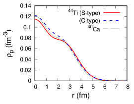
Figure 1: Point-proton density distributions of ⁴⁴Ti and ⁴⁰Ca. The distributions are the same for neutron.

Figure 1 displays the point-proton density distributions (S-type and C-type) of ⁴⁴Ti. Note that the distributions are the same for the neutrons. The density distribution of ⁴⁰Ca is also plotted for comparison. Despite that the S-type and C-type density distributions give the same charge radii, they exhibit different density profiles. All three densities coincide at $r\approx 3$ fm, which divides the internal and outer parts of the density distribution. The internal densities are reduced in the S-type. This is attributed to the fact that in S-type, the increase of the charge radius from ⁴⁰Ca to ⁴⁴Ti partially comes from the change of the size of the oscillator parameter, $1/\sqrt{\nu}$. This leads to the depression of the internal density. For the C-type, the internal density at around $r\approx 1$–3 fm is enhanced, which is reasonable, given the $\alpha$ cluster is located at $r\approx 3$ fm. Around the surface regions, at $r\gtrsim 3$ fm the S-type density has larger values, but the inversion occurs, and the C-type density is larger at $r\gtrsim 4$ fm.

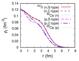
Figure 2: Point-proton ($t=p$) and neutron ($t=n$) density distributions of ⁵²Ti and ⁴⁸Ca.

Figure 2 plots the point-proton and neutron density distributions of ⁵²Ti and ⁴⁸Ca. The charge radius of ⁵⁰Ti is used for ⁵²Ti to determine the parameters. While changes in the proton density distributions from ⁴⁸Ca to ⁵²Ti are small, they are similar to these for the ⁴⁴Ti case. For the neutron density distributions, though the densities at the surface region of $r\gtrsim 4$ fm is a little enhanced, the S- and C-type distributions are quite similar, implying the effect of the $(0f_{7/2})_{n}^{8}$ configuration in the ⁴⁸Ca part. We will address this reason in the next subsection.

These differences between the S-type and C-type are reflected in patterns of proton-nucleus diffraction. Figure 3 plots the proton-nucleus differential elastic scattering cross sections. The proton incident energies are chosen as at 320 and 1000 MeV, where the experimental data of ${}^{40,48}{\rm Ca}+p$ is available [65, 66, 67] (crosses). Our results perfectly reproduce the data of ${}^{40,48}{\rm Ca}+p$ up to the second peak, which verifies our approach. For ⁴⁴Ti, the difference between the two types of density models (S-type and C-type) is apparent at the first and second peak positions. For a closer comparison, we plot in Fig. 4 the cross sections in a linear scale. We clearly see that the difference between the cross sections of the S-type and C-type density models is larger than the uncertainties of the experimental ${}^{40}{\rm Ca}+p$ cross sections at the first peak position. Measurement of these cross sections is useful to distinguish the degree of the clustering near the nuclear surface. In contrast, less difference is found in the cases of ⁵²Ti as expected from Fig. 2. The difference is found to be comparable to the uncertainties of the experimental ${}^{48}{\rm Ca}+p$ cross sections. The situation is improved when we take the extended charge radius for ⁵²Ti.

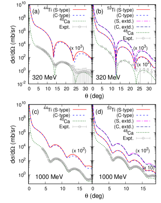
Figure 3: Differential elastic scattering cross sections of (a,c) ${}^{44}{\rm Ti}+p$ and ${}^{40}{\rm Ca}+p$ and (b,d) ${}^{52}{\rm Ti}+p$ and ${}^{48}{\rm Ca}+p$ at incident energies of (a,b) 320 MeV and (c,d) 1000 MeV as a function of scattering angles. The experimental data is taken from Refs. [65, 66, 67]. For the sake of visibility, the cross sections of ${}^{44}{\rm Ti}+p$ and ${}^{52}{\rm Ti}+p$ are multiplied by some factors.

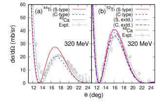
Figure 4: Same as Fig. 3 (a) and (b) but in a linear scale.

These differences in the density profiles can also influence the total reaction cross sections. Figure 5 displays the calculated total reaction cross sections as a function of the incident energy. Though the difference is not as significant as that in the proton-nucleus differential elastic scattering cross sections, the difference between the two density models (S-type and C-type) is at most about 2% for ⁴⁴Ti, which is larger than the present experimental precision, typically less than 1% [62, 68]. The cross sections with the S- and C-type density distributions are almost identical for ⁵²Ti. A little difference is found when the extended charge radius is applied to ⁵²Ti.

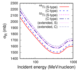
Figure 5: Total reaction cross sections of ⁴⁴Ti and ⁵²Ti on a carbon target as a function of incident energy.

To explore the $\alpha$-clustering for heavier nuclei, we investigate cases for Sn isotopes; to be more specific, ${}^{120}{\rm Sn}+\alpha$ and ${}^{132}{\rm Sn}+\alpha$. We found that The C-type configuration always gives more diffused nuclear surface than that of S-type as we have shown in Ti isotopes. However, the density profiles of the S- and C-types becomes similar as the mass number increases that cannot be distinguished clearly. In such a case, a more direct way, e.g., $\alpha$-knockout reaction [19] could be more useful to quantify the degree of the $\alpha$ clustering.

III.3 Close comparison of the density profiles

To clarify the origin of the differences in the density profiles, it is convenient to quantify the density profiles near the nuclear surface. For this purpose, we extract the nuclear diffuseness from the calculated density distributions using the prescription given in Ref. [15]. Nuclear diffuseness is defined in a two-parameter Fermi (2pF) function

$$\rho_{\rm 2pF}(\bar{R}_{q},a_{q},r)=\frac{\rho_{0q}}{1+\exp[(r-\bar{R}_{q})/a_{q}]},$$ (15)

where the radius $\bar{R}_{q}$ and diffuseness $a_{q}$ parameters are respectively defined for neutron $(q=n)$, proton $(q=p)$, and matter ($q=m$). Given the $\bar{R}_{q}$ and $a_{q}$ values, the $\rho_{0q}$ value is uniquely determined by the normalization condition. These parameters are determined by minimizing

$$\int_{0}^{\infty}dr\,r^{2}\left|\rho_{\rm 2pF}(\bar{R}_{q},a_{q},r)-\rho_{q}(r)\right|.$$ (16)

Note $\rho_{m}=\rho_{p}+\rho_{n}$. The extracted 2pF parameters are equivalent to those obtained by fitting the first peak position and its magnitude of proton-nucleus elastic scattering [15, 17, 16].

Table 2 also lists the extracted diffuseness parameters for proton, neutron, and matter density distributions. These values capture well the characteristics of the density distributions. The diffuseness parameters are similar for ⁴⁰Ca and ⁴⁴Ti (S-type), while it is significantly enhanced for ⁴⁴Ti (C-type). In the case of ⁵²Ti, both the S- and C-types shows enhanced diffuseness parameters for neutron and matter, while for proton, a similar behavior is found as that for ⁴⁴Ti.

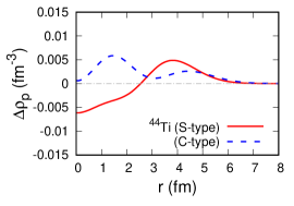
Figure 6: Difference of point-proton density distributions between ⁴⁴Ti and ⁴⁰Ca.

To verify the reason, we plot in Fig. 6 the difference of the proton density distributions between ⁴⁴Ti and ⁴⁰Ca as a function of $r$, i.e., $\Delta\rho_{p}(r)=\rho_{p}(^{44}{\rm Ti},r)-\rho_{p}(^{40}{\rm Ca},r)$. In the S-type, the internal density is depressed reflecting the difference of the oscillator parameters of these nuclei. It peaks at $r\approx 4$ fm coming from the additional $(0f_{7/2})_{p}^{2}$ configuration. The $\Delta\rho_{p}(r)$ value of the C-type behaves quite differently, showing two peak structure that indicates the inclusion of the nodal $1p$ orbits, which significantly enhances the diffuseness of the nuclear surface [69]. The four valence nucleons mainly occupy a “sharp” $0f_{7/2}$ orbit in the S-type density, while a “diffused” $1p$ orbit is filled in the C-type density, leading to the significant difference in the density profiles near the nuclear surface.

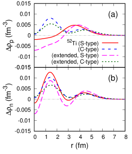
Figure 7: Difference of the density distributions for (a) proton and (b) neutron between ⁵²Ti from ⁴⁸Ca.

For ⁴⁸Ca, the diffuseness parameter is smaller than that of ⁴⁰Ca as the sharp $0f_{7/2}$ neutron orbit is filled as seen in Table 2. Differently from the ⁴⁴Ti case, in ⁵²Ti, the neutron diffuseness is enhanced also for the S-type because the two valence neutrons are considered to occupy the $1p_{3/2}$ orbit; $0f_{7/2}$ orbits for the neutrons are fully occupied in the ⁴⁸Ca core. This effect leads to the enhancement of nuclear diffuseness. Figure 7 plots the differences of the proton and neutron density distributions between ⁵²Ti and ⁴⁸Ca. The C-type density of ⁵²Ti behaves like ⁴⁴Ti but the amplitudes in the internal region are larger because the resulting core-$\alpha$ distance is smaller than that of ⁴⁴Ti as we see in Table 1. We also calculate the $\Delta\rho_{p}$ and $\Delta\rho_{n}$ for the extended ⁵²Ti density distributions. The enhancement of the surface region is more apparent relative to that of the internal region and the behavior of $\Delta\rho_{p}$ becomes closer to that of ⁴⁴Ti.

In summary, the C-type density gives a more diffused surface than that of the S-type in ⁴⁴Ti because the cluster configuration allows the occupation of the nodal $1p$ orbit both for neutrons and protons. For ⁵²Ti, both the S- and C-types induce the enhancement of the diffuseness because the S-type also fills in the $1p_{3/2}$ orbit due to the Pauli principle from the ⁴⁸Ca core. The difference in the density profiles for the S- and C-type configurations is found to be less drastic than in the case of ⁴⁴Ti. Investigation of the spectroscopic properties of these nuclei can corroborate this scenario, which can be achieved by using, e.g., the nucleon(s) knockout reactions [70].

IV Conclusion

We have studied the degree of the $\alpha$ clustering in the ground state of ⁴⁴Ti and ⁵²Ti by using fully antisymmetrized wave functions, antisymmetrized quasi-cluster model (AQCM), which can describe both the shell and cluster configurations in a single scheme. The characteristics of the density profiles are elucidated by assuming the shell-model and $\alpha$-cluster-like configurations. The nuclear surface is diffused by nodal single-particle orbits induced by localized four-nucleons at the nuclear surface. The difference between the shell and cluster configurations becomes apparent for ⁴⁴Ti, while it is less for ⁵²Ti because the shell model configuration also has a diffused nuclear surface originating from the $1p_{3/2}$ orbit due to the Pauli principle between the excess neutrons.

In this paper, we show two limits of shell and cluster configurations and find that these two aspects can be distinguished by measuring the proton-nucleus elastic differential cross section up to the first peak position as well as the nucleus-nucleus total reaction cross sections. In reality, a nucleus consists of a mixture of these two limits. Thus, these measurements will tell us dominant configurations of the projectile nucleus, which offers a complementary tool to quantify the existence of $\alpha$ cluster near the nuclear surface.

- [1] R. Hofstadter, Rev. Mod. Phys. 28, 214 (1956).
- [2] H. Sakaguchi and J. Zenihiro, Prog. Part. Nucl. Phys. 97, 1 (2017), and references therein.
- [3] Y. Matsuda, H. Sakaguchi, H. Takeda, S. Terashima, J. Zenihiro, T. Kobayashi, T. Murakami, Y. Iwao, T. Ichihara, T. Suda et al., Phys. Rev. C 87, 034614 (2013).
- [4] W. Horiuchi and T. Inakura, Phys. Rev. C 101, 061301(R) (2020).
- [5] W. Horiuchi and T. Inakura, Prog. Theor. Exp. Phys. 2021, 103D02 (2021).
- [6] M. Takechi, T. Ohtsubo, M. Fukuda, D. Nishimura, T. Kuboki, T. Kubo, T. Suzuki, T. Yamaguchi, A. Ozawa, T. Moriguchi, H. Ooishi, Phys. Lett. B 707, 357 (2012).
- [7] M. Takechi, S. Suzuki, D. Nishimura, M. Fukuda, T. Ohtsubo, M. Nagashima, T. Suzuki, T. Yamaguchi, A. Ozawa, T. Moriguchi et al., Phys. Rev. C 90, 061305(R) (2014).
- [8] K. Minomo, T. Sumi, M. Kimura, K. Ogata, Y. R. Shimizu, and M. Yahiro, Phys. Rev. C 84, 034602 (2011).
- [9] K. Minomo, T. Sumi, M. Kimura, K. Ogata, Y. R. Shimizu, and M. Yahiro, Phys. Rev. Lett. 108, 052503 (2012).
- [10] T. Sumi, K. Minomo, S. Tagami, M. Kimura, T. Matsumoto, K. Ogata, Y. R. Shimizu, and M. Yahiro, Phys. Rev. C 85, 064613 (2012).
- [11] W. Horiuchi, T. Inakura, T. Nakatsukasa, and Y. Suzuki, Phys. Rev. C 86, 024614 (2012).
- [12] S. Watanabe, K. Minomo, M. Shimada, S. Tagami, M. Kimura, M. Takechi, M. Fukuda, D. Nishimura, T. Suzuki, T. Matsumoto et al., Phys. Rev. C 89, 044610 (2014).
- [13] W. Horiuchi, T. Inakura, T. Nakatsukasa, and Y. Suzuki, JPS Conf. Proc. 6, 030079 (2015).
- [14] W. Horiuchi, T. Inakura, and S. Michimasa, Phys. Rev. C 105, 014316 (2022).
- [15] S. Hatakeyama, W. Horiuchi, and A. Kohama, Phys. Rev. C 97, 054607 (2018).
- [16] V. Choudhary, W. Horiuchi, M. Kimura, and R. Chatterjee, Phys. Rev. C 104, 054313 (2021).
- [17] V. Choudhary, W. Horiuchi, M. Kimura, and R. Chatterjee, Phys. Rev. C 102, 034619 (2020).
- [18] S. Typel, G. Röpke, T. Klähn, D. Blaschke, and H. H. Wolter, Phys. Rev. C 81, 015803 (2010).
- [19] J. Tanaka, Z. Yang, S. Typel, S. Adachi, S. Bai, P. van Beek, D. Beaumel, Y. Fujikawa, J. Han, S. Heil et al., Science 371, 260 (2021).
- [20] F. Michel, G. Reidemeister, and S. Ohkubo, Phys. Rev. Lett. 57, 1215 (1986).
- [21] T. Yamaya, S. Oh-ami, M. Fujiwara, T. Itahashi, K. Katori, M. Tosaki, S. Kato, S. Hatori, and S. Ohkubo, Phys. Rev. C 42, 1935 (1990).
- [22] T. Yamaya, K. Katori, M. Fujiwara, S. Kato, and S. Ohkubo, Prog. Theor. Phys. Suppl. 132, 73 (1998).
- [23] M. Kimura and H. Horiuchi, Nucl. Phys. A 767, 58 (2006).
- [24] H. Nassar, M. Paul, I. Ahmad, Y. Ben-Dov, J. Caggiano, S. Ghelberg, S. Goriely, J. P. Greene, M. Hass, A. Heger, A. Heinz, D. J. Henderson, R. V. F. Janssens, C. L. Jiang, Y. Kashiv, B. S. NaraSingh, A. Ofan, R. C. Pardo, T. Pennington, K. E. Rehm, G. Savard, R. Scott, and R. Vondrasek, Phys. Rev. Lett. 96, 041102 (2006).
- [25] Y. Taniguchi, K. Yoshida, Y. Chiba, Y. Kanada-En’yo, M. Kimura, and K. Ogata, Phys. Rev. C 103, L031305 (2021).
- [26] C. Ishizuka, H. Takemoto, Y. Chiba, A. Ono, and N. Itagaki, Phys. Rev. C 105, 064314 (2022).
- [27] N. Itagaki, H. Masui, M. Ito, and S. Aoyama, Phys. Rev. C 71, 064307 (2005).
- [28] H. Masui and N. Itagaki, Phys. Rev. C 75, 054309 (2007).
- [29] T. Yoshida, N. Itagaki, and T. Otsuka, Phys. Rev. C 79, 034308 (2009).
- [30] N. Itagaki, J. Cseh, and M. Płoszajczak, Phys. Rev. C 83, 014302 (2011).
- [31] T. Suhara, N. Itagaki, J. Cseh, and M. Płoszajczak, Phys. Rev. C 87, 054334 (2013).
- [32] N. Itagaki, H. Matsuno, and T. Suhara, Prog. Theor. Exp. Phys. 2016, 093D01 (2016).
- [33] H. Matsuno, N. Itagaki, T. Ichikawa, Y. Yoshida, and Y. Kanada-En’yo, Prog. Theor. Exp. Phys. 2017, 063D01 (2017).
- [34] H. Matsuno and N. Itagaki, Prog. Theor. Exp. Phys. 2017, 123D05 (2017).
- [35] N. Itagaki, Phys. Rev. C 94, 064324 (2016).
- [36] N. Itagaki and A. Tohsaki, Phys. Rev. C 97, 014307 (2018).
- [37] N. Itagaki, H. Matsuno, and A. Tohsaki, Phys. Rev. C 98, 044306 (2018).
- [38] N. Itagaki, A. V. Afanasjev, and D. Ray, Phys. Rev. C 101, 034304 (2020).
- [39] N. Itagaki, T. Fukui, J. Tanaka, and Y. Kikuchi, Phys. Rev. C 102, 024332 (2020).
- [40] N. Itagaki and T. Naito, Phys. Rev. C 103, 044303 (2021).
- [41] M. Brink, Proc. Int. School Phys.“Enrico Fermi” XXXVI,, 247 (1966).
- [42] J. L. Friar, J. Martorell, and D. W. L. Sprung, Phys. Rev. A 56, 4579 (1997).
- [43] I. Angeli and K. P. Marinova, At. Data Nucl. Data Tables 99, 69 (2013).
- [44] S. Terashima, H. Sakaguchi, H. Takeda, T. Ishikawa, M. Itoh, T. Kawabata, T. Murakami, M. Uchida, Y. Yasuda, M. Yosoi et al., Phys. Rev. C 77, 024317 (2008).
- [45] J. Zenihiro, H. Sakaguchi, T. Murakami, M. Yosoi, Y. Yasuda, S. Terashima, Y. Iwao, H. Takeda, M. Itoh, H. P. Yoshida, and M. Uchida, Phys. Rev. C 82, 044611 (2010).
- [46] R. J. Glauber, Lectures in Theoretical Physics, edited by W. E. Brittin and L. G. Dunham (Interscience, New York, 1959), Vol. 1, p.315.
- [47] Y. Suzuki, R. G. Lovas, K. Yabana, K. Varga, Structure and reactions of light exotic nuclei (Taylor & Francis, London, 2003) .
- [48] B. Abu-Ibrahim, W. Horiuchi, A. Kohama, and Y. Suzuki, Phys. Rev. C 77, 034607 (2008); ibid 80, 029903(E) (2009); 81, 019901(E) (2010).
- [49] W. Horiuchi, S. Hatakeyama, S. Ebata, and Y. Suzuki, Phys. Rev. C 93, 044611 (2016).
- [50] K. Varga, S. C. Pieper, Y. Suzuki, and R. B. Wiringa, Phys. Rev. C 66, 034611 (2002).
- [51] B. Abu-Ibrahim, S. Iwasaki, W. Horiuchi, A. Kohama, and Y. Suzuki, J. Phys. Soc. Jpn., Vol. 78, 044201 (2009).
- [52] T. Nagahisa and W. Horiuchi, Phys. Rev. C 97, 054614 (2018).
- [53] S. Hatakeyama and W. Horiuchi, Nucl. Phys. A 985, 20 (2019).
- [54] W. Horiuchi, Y. Suzuki, and T. Inakura, Phys. Rev. C 89, 011601(R) (2014).
- [55] K. Makiguchi and W. Horiuchi, Prog. Theor. Exp. Phys. 2022, 073D01 (2022).
- [56] B. Abu-Ibrahim and Y. Suzuki, Phys. Rev. C 61, 051601(R) (2000).
- [57] W. Horiuchi and Y. Suzuki, Phys. Rev. C 74, 034311 (2006).
- [58] W. Horiuchi, Y. Suzuki, B. Abu-Ibrahim, and A. Kohama, Phys. Rev. C 75, 044607 (2007); ibid 76, 039903(E) (2007).
- [59] W. Horiuchi, Y. Suzuki, P. Capel, and D. Baye, Phys. Rev. C 81, 024606 (2010).
- [60] R. Kanungo, A. Prochazka, W. Horiuchi, C. Nociforo, T. Aumann, D. Boutin, D. Cortina-Gil, B. Davids, M. Diakaki, F. Farinon et al., Phys. Rev. C 83, 021302(R) (2011).
- [61] R. Kanungo, A. Prochazka, W. Horiuchi, C. Nociforo, T. Aumann, D. Boutin, D. Cortina-Gil, B. Davids, M. Diakaki, F. Farinon et al., Phys. Rev. C 83, 021302(R) (2011).
- [62] S. Bagchi, R. Kanungo, Y. K. Tanaka, H. Geissel, P. Doornenbal, W. Horiuchi, G. Hagen, T. Suzuki, N. Tsunoda, D. S. Ahn et al., Phys. Rev. Lett. 124, 222504 (2020).
- [63] W. Horiuchi and Y. Suzuki, Phys. Rev. C , 89, 011304(R) (2014).
- [64] Q, Zhao, Y. Suzuki, J. He, B. Zhou, and M. Kimura, Eur. Phys. J A 57, 157 (2021).
- [65] G. D. Alkhazov, T. Bauer, R. Beurtey, A. Boudard, G. Bruge, A. Chaumeaux, P. Couvert, G. Cvijanovich, H. H. Duhm, J. M. Fontaine et al., Nucl. Phys. A 274, 443 (1976).
- [66] J. J. Kelly, P. Boberg, A. E. Feldman, B. S. Flanders, M. A. Khandaker, S. D. Hyman, H. Seifert, P. Karen, B. E. Norum, P. Welch, S. Nanda, and A. Saha, Phys. Rev. C 44, 2602 (1991).
- [67] A. E. Feldman, J. J. Kelly, B. S. Flanders, M. A. Khandaker, H. Seifert, P. Boberg, S. D. Hyman, P. Karen, B. E. Norum, P. Welch et al., Phys. Rev. C 49, 2068 (1994).
- [68] M. Tanaka, M. Takechi, M. Fukuda, D. Nishimura, T. Suzuki, Y. Tanaka, T. Moriguchi, D. S. Ahn, A. Aimaganbetov, M. Amano et al., Phys. Rev. Lett. 124, 102501 (2020).
- [69] W. Horiuchi, Prog. Theor. Exp. Phys. 2021, 123D01 (2021).
- [70] A. Gade and T. Glasmacher, Prog. Part. Nucl. Phys. 60, 161 (2008) and references therein.