Deep Fourier Up-Sampling

Abstract

Existing convolutional neural networks widely adopt spatial down-/up-sampling for multi-scale modeling. However, spatial up-sampling operators (e.g., interpolation, transposed convolution, and un-pooling) heavily depend on local pixel attention, incapably exploring the global dependency. In contrast, the Fourier domain obeys the nature of global modeling according to the spectral convolution theorem. Unlike the spatial domain that performs up-sampling with the property of local similarity, up-sampling in the Fourier domain is more challenging as it does not follow such a local property. In this study, we propose a theoretically sound Deep Fourier Up-Sampling (FourierUp) to solve these issues. We revisit the relationships between spatial and Fourier domains and reveal the transform rules on the features of different resolutions in the Fourier domain, which provide key insights for FourierUp’s designs. FourierUp as a generic operator consists of three key components: 2D discrete Fourier transform, Fourier dimension increase rules, and 2D inverse Fourier transform, which can be directly integrated with existing networks. Extensive experiments across multiple computer vision tasks, including object detection, image segmentation, image de-raining, image dehazing, and guided image super-resolution, demonstrate the consistent performance gains obtained by introducing our FourierUp.

1 Introduction

Spatial down-/up-sampling has been widely used in convolutional neural networks for multi-scale modeling. For example, U-Net [1], a variation of encoder-decoder, employs pooling layers to reduce the feature resolution in the encoder and then recovers the resolution using up-sampling operations in the decoder. In addition, the feature pyramid [2, 3, 4, 5] and image pyramid [6, 7, 8, 9] driven multi-scale neural networks rely on the down-/up-sampling operation to obtain multi-scale property and improve modeling capability. However, spatial up-sampling operators (e.g., interpolation, transposed convolution, and un-pooling) heavily depend on local pixel attention, and thus cannot explore the global dependency that is indispensable for many computer vision tasks [10, 11, 1, 12, 13, 14, 15, 16, 17, 18, 19, 20]. According to the spectral convolution theorem, the Fourier domain obeys the nature of global modeling, providing an alternative solution for multi-scale modeling. However, unlike the spatial domain with local similarity property, up-sampling in the Fourier domain is more challenging as it does not follow such a local property. The observation encourages us to explore deep Fourier up-sampling.

Recent studies have explored information interaction in both spatial and Fourier domains. FFC [21], for instance, replaces the conventional convolution with a spatial-Fourier interaction, which consists of a spatial (or local) path that performs conventional convolution on a portion of input feature channels and a spectral (or global) path that operates in the Fourier domain. DFT [22] devises a Residual Fast Fourier Transform Block to integrate both low- and high-frequency residual information by performing the interaction between a regular spatial residual stream and a channel-wise Fourier transform stream. However, the aforementioned methodologies only interact at a single resolution scale, and the spatial-Fourier interaction potential of multiple scales in the Fourier domain has not been investigated. The key to solving this problem lies in how to implement deep Fourier up-sampling for multi-scale Fourier pattern modeling.

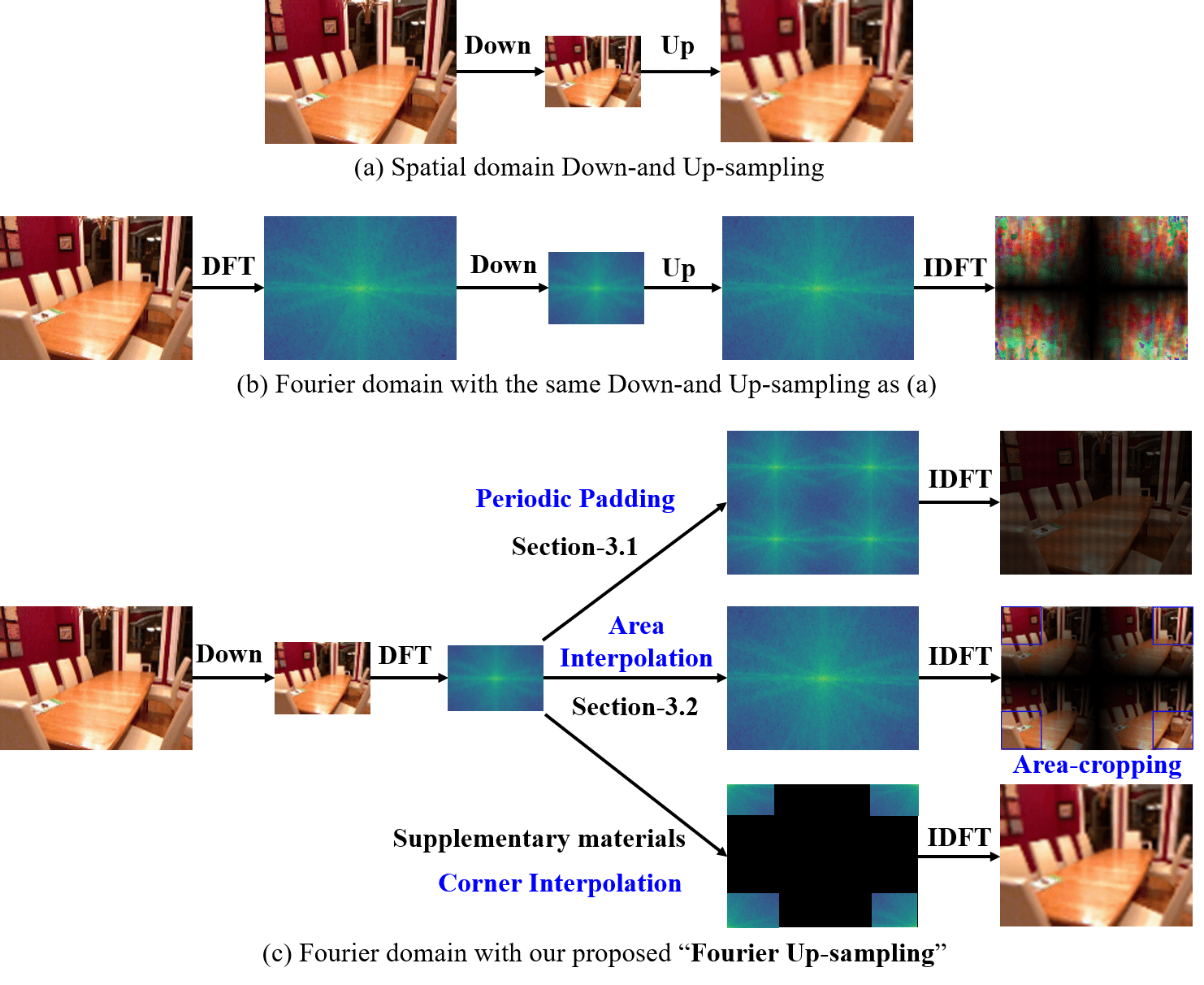
Figure 1: Motivation. (a) and (b) depict that arbitrary up-sampling, e.g., interpolation, in the Fourier domain produces sub-optimal result as it does not follow the same local similarity property as that in the spatial domain. This motivates us to design a more ingenious “Fourier Up-Sampling” operator, dubbed as FourierUp. It has three alternative variants: Periodic Padding, Area Interpolation/Cropping and Corner Interpolation, as illustrated in (c).

Challenges. Owing to the local similarity and cross-scale position invariant properties of the spatial domain, the various spatial up-sampling operations including transposed convolution, un-pooling, and interpolation techniques are capable of using the pixel neighboring relationship to interpolate the unknown pixel values at local regions, increasing the spatial resolution of the features, as shown in Figure 1(a). In contrast to the spatial domain, the Fourier domain does not share the same scale-invariant property and local texture similarity, and hence cannot implement up-sampling using the same techniques as the spatial domain, as illustrated in Figure 1(b).

Solutions. In this paper, we wish to investigate the possibility of devising a reliable up-sampling in the Fourier domain in a theoretical sound manner. To answer this question, we first revisit the relationship between spatial and Fourier domains, revealing the transform rules on the features of different resolutions in the Fourier domain (see Section 3.1 and Section 3.2). On the basis of the above rules, we propose a theoretically feasible Deep Fourier Up-Sampling (FourierUp). Specifically, we develop three variants (Periodic Padding, Area Interpolation/Cropping and Corner Interpolation) of FourierUp (see Section 3.3), as illustrated in Figure 1(c). Each variant consists of three key components: 2D discrete Fourier transform, Fourier dimension increase rules, and 2D inverse Fourier transform. FourierUp is a generic operator that can be directly integrated with existing networks. Extensive experiments on multiple computer vision tasks, including object detection, image segmentation, image de-raining, image dehazing, and guided image super-resolution, demonstrate the consistent performance gains obtained by introducing our FourierUp. We believe that the proposed FourierUp could refresh the neural network designs where the spatial and Fourier information interaction at only a single resolution scale are mainstream choices.

Contributions. 1) We propose Deep Fourier Up-Sampling, a novel method that enables the integration of the features of different resolutions in the Fourier domain. This is the first thorough effort to explore the Fourier up-sampling for multi-scale modeling. 2) The proposed FourierUp is a generic operator that can be directly integrated with the existing networks in a plug-and-play manner. 3) Equipped with the theoretically sound FourierUp, we show that existing networks could achieve consistent performance improvement across multiple computer vision tasks.

2 Related Work

Spatial Up-Sampling. Convolutional neural networks with spatial down-/up-sampling have become the de facto structures in many computer vision tasks [23, 24, 25, 26, 27, 28, 29, 30, 31]. Typically, U-Net [1] builds multi-scale feature maps using the encoder with down-sampling and then utilizes the up-sampling operation to fuse the multi-scale features in the decoder. Additionally, the feature pyramid [2, 3, 4, 5] and image pyramid[6, 7, 8, 9] are commonly used to obtain the multi-scale property in neural networks [6, 7, 8, 9]. Among them, spatial up-sampling plays a significant role in multi-scale modeling. However, existing up-sampling operations only work in the spatial domain and current studies rarely explore the potential (e.g., the global modeling capability) of up-sampling in the frequency domain.

Spatial-Fourier Interaction. Recently, several studies attempt to employ Fourier transform in deep models [32, 33, 34, 35, 21]. Some of these efforts use discrete Fourier transform to transfer the spatial features to the Fourier domain and then use frequency information to improve the performance of particular tasks [32, 34]. Another line is to use convolution theorem to speed up the models, such as using fast Fourier transform (FFT) [35, 21]. For example, FFC [21] replaces the convolution with the spatial-Fourier interaction. The work proposed in [36] uses spectral pooling to reduce feature resolution by truncating the frequency domain representation. However, all the techniques only interact with each other at a single spatial resolution and have not explored the interaction potential at multiple resolutions in both spatial and frequency domains as performing the frequency up-sampling is non-trivial. As a tentative exploration, we study the relationship between the spatial domain and Fourier domain and reveal the transform rules over the feature of different resolutions in the Fourier domain. This delivers the underlying insights for the designs of multi-scale Fourier modeling patterns, which has the potential of versatility for different network architectures.

3 Deep Fourier Up-Sampling

We first explore the mapping relationship between the spatial and Fourier domains, and then present three Deep Fourier up-sampling variants, including i) periodic padding of magnitude and phase, ii) area up-sampling of magnitude and phase, and iii) corner interpolation of magnitude and phase, based on the explored transform rules. In terms of the first two variants, we provide two theorems and their proofs as follows while the third is reported in supplementary materials.

Definitions. $f(x,y)\in\mathbb{R}^{2M\times 2N}$ is the $2$-times zero-inserted up-sampled version of $g(x,y)\in\mathbb{R}^{M\times N}$ in spatial domain, and $F(u,v)\in\mathbb{R}^{2M\times 2N}$, $G(u,v)\in\mathbb{R}^{M\times N}$ denote their Fourier transforms. $H(u,v)\in\mathbb{R}^{2M\times 2N}$ is the $2$-times area-interpolation up-sampled Fourier transform of $G(u,v)$, and $h(x,y)\in\mathbb{R}^{M\times N}$ denotes their inverse Fourier transform.

Theorem-1. $F(u,v)=F(u+M,v)=F(u,v+N)=F(u+M,v+N)$ and $G(u,v)=\frac{F(u,v)}{4}$ where $u=0,1,2,\dots,N-1$ and $v=0,1,2,\dots,M-1$. $F(u,v)$ is exactly the periodic padding of $G(u,v)$ where $G(u,v)$ is exactly the quarter of $F(u,v)$ with the value being $\frac{1}{4}$ times decay.

Theorem-2. $H(2u,2v)=H(2u+1,2v)=H(2u,2v+1)=H(2u+1,2v+1)=G(u,v)$ with $u=0,1,\dots,M-1$ and $v=0,1,\dots,N-1$ and

$$h(x,y) =\frac{A(x,y)}{4}g(x,y)$$ (1)

$$h(x+M,y) =\frac{A(2M-x,y)}{4}g(x,y)$$

$$h(x,y+N) =\frac{A(x,2N-y)}{4}g(x,y)$$

$$h(x+M,y+N) =\frac{A(2M-x,2N-y)}{4}g(x,y)$$

where $A(x,y)=1+e^{\frac{j\pi x}{M}}+e^{\frac{j\pi y}{N}}+e^{j\pi(\frac{x}{M}+\frac{y}{N})}$ and $x=0,1,\dots M-1,y=0,1,\dots N-1$.

Theorem-3. Suppose the corner interpolated $F^{cor}_{G}(u,v)$ of the Fourier map $G(u,v)\in\mathbb{R}^{M\times N}$, it holds that the inverse Fourier transform $f^{cor}_{g}(x,y)$ of $F^{cor}_{G}(u,v)$

$$f^{cor}_{g}(x,y)=g(\frac{x^{\prime}}{2},\frac{y^{\prime}}{2})e^{j\pi(\frac{x^{\prime}}{2}+\frac{y^{\prime}}{2})}\frac{(-1)^{(x+y)}}{4},$$ (2)

where $x^{\prime}=2x$ and $y^{\prime}=2y$, $x=0,1,\dots,M-1$ and $y=0,1,\dots,N-1$.

3.1 Proof-1 of Theorem-1: Periodic Padding of Magnitude and Phase

Note that $f(x,y)\in\mathbb{R}^{2M\times 2N}$ is up-sampled over $g(x,y)\in\mathbb{R}^{M\times N}$ by a factor of $2$. The relationship between $g(x,y)$ and $f(x,y)$ can be written as

$$\boldsymbol{f}(x,y) = \left\{\begin{array}[]{l}g(\frac{x}{2},\frac{y}{2}),\quad x=2m,y=2n\\ 0,\quad\quad\quad\quad\text{others}\end{array}\right.$$ (5)

where $m=1,2,\dots,M-1$ and $n=1,2,\dots,N-1$, the Fourier transform $F(u,v)$ of $f(x,y)$ is expressed as

$$F(u,v) =\frac{1}{4MN}\sum_{x=0}^{2M-1}\sum_{y=0}^{2N-1}f(x,y)e^{-j2\pi(\frac{ux}{2M}+\frac{vy}{2N})}$$ (6)

$$=\frac{1}{4MN}\sum_{x=0}^{M-1}\sum_{y=0}^{N-1}f(2x,2y)e^{-j2\pi(\frac{u(2x)}{2M}+\frac{v(2y)}{2N})}$$

$$=\frac{1}{4MN}\sum_{x=0}^{M-1}\sum_{y=0}^{N-1}f(2x,2y)e^{-j2\pi(\frac{ux}{M}+\frac{vy}{N})}$$

$$=\frac{1}{4MN}\sum_{x=0}^{M-1}\sum_{y=0}^{N-1}g(x,y)e^{-j2\pi(\frac{ux}{M}+\frac{vy}{N})}.$$

Then, we show the periodicity of $F(u,v)\in R^{2M\times 2N}$ with $M$ and $N$. It means $F(u,v)=F(u+M,v)=F(u,v+N)=F(u+M,v+N)$ with $u=0,1,2,\dots,N-1$ and $v=0,1,2,\dots,M-1$. We take the $F(u,v)=F(u+M,v)$ for example and recall Eq. (6) as

$$F(u+M,v) =\frac{1}{4MN}\sum_{x=0}^{M-1}\sum_{y=0}^{N-1}f(2x,2y)e^{-j2\pi(\frac{(u+M)x}{M}+\frac{vy}{N})}$$ (7)

$$=\frac{1}{4MN}\sum_{x=0}^{M-1}\sum_{y=0}^{N-1}f(2x,2y)e^{-j2\pi(\frac{(ux}{M}+\frac{vy}{N})}e^{-2j\pi x}$$

$$=\frac{1}{4MN}\sum_{x=0}^{M-1}\sum_{y=0}^{N-1}f(2x,2y)e^{-j2\pi(\frac{(ux}{M}+\frac{vy}{N})}$$

$$=F(u,v),$$

where $e^{-2\pi jx}=1$ for any integer $x$. Similarly, we can proof the periodicity of $F(u,v)$ as well.

Based on the above proof, the DFT of $g(x,y)$ can be formulated as:

$$G(u,v) =\frac{1}{MN}\sum_{x=0}^{M-1}\sum_{y=0}^{N-1}g(x,y)e^{-j2\pi(\frac{ux}{M}+\frac{vy}{N})}.$$ (8)

Revising Eq. (6), we can figure out that $G(u,v)=\frac{F(u,v)}{4}$.

3.2 Proof-2 of Theorem-2: Area Interpolation of Magnitude and Phase

The 2D Inverse Discrete Fourier transform (IDFT) of $G(u,v)$ can be written as:

$$g(x,y)=\frac{1}{MN}\sum_{u=0}^{M-1}\sum_{v=0}^{N-1}G(u,v)e^{j2\pi(\frac{ux}{M}+\frac{vy}{N})}.$$ (9)

We up-sample $G(u,v)$ with a size of $M\times N$ to get $H(u,v)$ with a size of $2M\times 2N$. Specifically, the area interpolation shown in Figure 3(b) is used for interpolation and then the interpolated pixels are the same as the original pixel in the $2\times 2$ local regions. Namely, $H(2u,2v)=H(2u+1,2v)=H(2u,2v+1)=H(2u+1,2v+1)=G(u,v)$ with $u=0,1,\dots,M-1$ and $v=0,1,\dots,N-1$. Similar to Eq. (6), we can infer

Similarly, we can write $g(x,y)$ as

$$g(x,y) =\frac{1}{MN}\sum_{u=0}^{M-1}\sum_{v=0}^{N-1}G(u,v)e^{j2\pi(\frac{ux}{M}+\frac{vy}{N})}.$$ (11)

Recalling Eq. (10) and Eq. (12), we can infer

$$h(x,y) =\frac{1+e^{\frac{j\pi x}{M}}+e^{\frac{j\pi y}{N}}+e^{j\pi(\frac{x}{M}+\frac{y}{N})}}{4}g(x,y).$$ (12)

where $x=0,1,\dots M-1,y=0,1,\dots N-1$. We remark $1+e^{\frac{j\pi x}{M}}+e^{\frac{j\pi y}{N}}+e^{j\pi(\frac{x}{M}+\frac{y}{N})}=A(x,y)$,

We can find that the variable $x$ shares the same operations as the variable $y$. For brevity, we only take the operation of variable $x$ as example

$$\frac{\partial\left|A(x,y)\right|^{2}}{\partial x} =\frac{2\pi}{M}(1+\cos\pi\frac{x}{M}+\cos\pi\frac{y}{N}+\cos\pi(\frac{x}{M}+\frac{y}{N}))(-\sin\pi\frac{x}{M}-\sin\pi(\frac{x}{M}+\frac{y}{N}))$$ (13)

$$+\frac{2\pi}{M}(\sin\pi\frac{x}{M}+\sin\pi\frac{y}{N}+\sin\pi(\frac{x}{M}+\frac{y}{N}))(\cos\pi(\frac{x}{M})+\cos\pi(\frac{x}{M}+\frac{y}{N}))$$

$$=-\frac{4\pi}{M}(\sin\pi\frac{x}{M})(1+\cos\pi(\frac{y}{N})).$$

Equally, we have

$$\frac{\partial\left|A(x,y)\right|^{2}}{\partial y} =-\frac{4\pi}{N}\sin\pi\frac{y}{N}(1+\cos\pi(\frac{x}{M})).$$ (14)

We prove that the partial derivative of $\left|A(x,y)\right|$ on both x and y is negative for $x\in[0,M-1]$ and $y\in[0,N-1]$. Besides, we have

$$\left|A(x,y)\right|=\left|A(2M-x,y)\right|=\left|A(2M,2N-y)\right|=\left|A(2M-x,2N-y)\right|.$$ (15)

That is to say, the intensity drops from the side to the center, shown in Figure 4. Specifically, the intensity drops to zero at the position of $x=M$ or $y=N$.

  ⬇ def DFU_Padding(X): # X: input with shape [N, C, H, W] # A and P are the amplitude and phase A, P = FFT(X) # Fourier up-sampling transform rules A_pep = Periodic-Padding(A) P_pep = Periodic-Padding(P) A_pep = Convs_1x1(A_pep) P_pep = Convs_1x1(P_pep) # Inverse Fourier transform Y = iFFT(A_pep, P_pep) Return Y #[N, C, 2H, 2W] ⬇ def DFU_AreaInterpolation(X): # X: input with shape [N, C, H, W] # A and P are the amplitude and phase A, P = FFT(X) # Fourier up-sampling transform rules A_aip = Area-Interpolation(A) P_aip = Area-Interpolation(P) A_aip = Convs_1x1(A_aip) P_aip = Convs_1x1(P_aip) # Inverse Fourier transform Y = iFFT(A_aip, P_aip) #Area Cropping Y = Area-Cropping(Y) Y = Resize(Y) Return Y #[N, C, 2H, 2W]

 

Figure 2: Pseudo-code of the two variants of the proposed deep Fourier up-sampling. The left is the periodic padding variant while the right is the area interpolation-cropping variant.

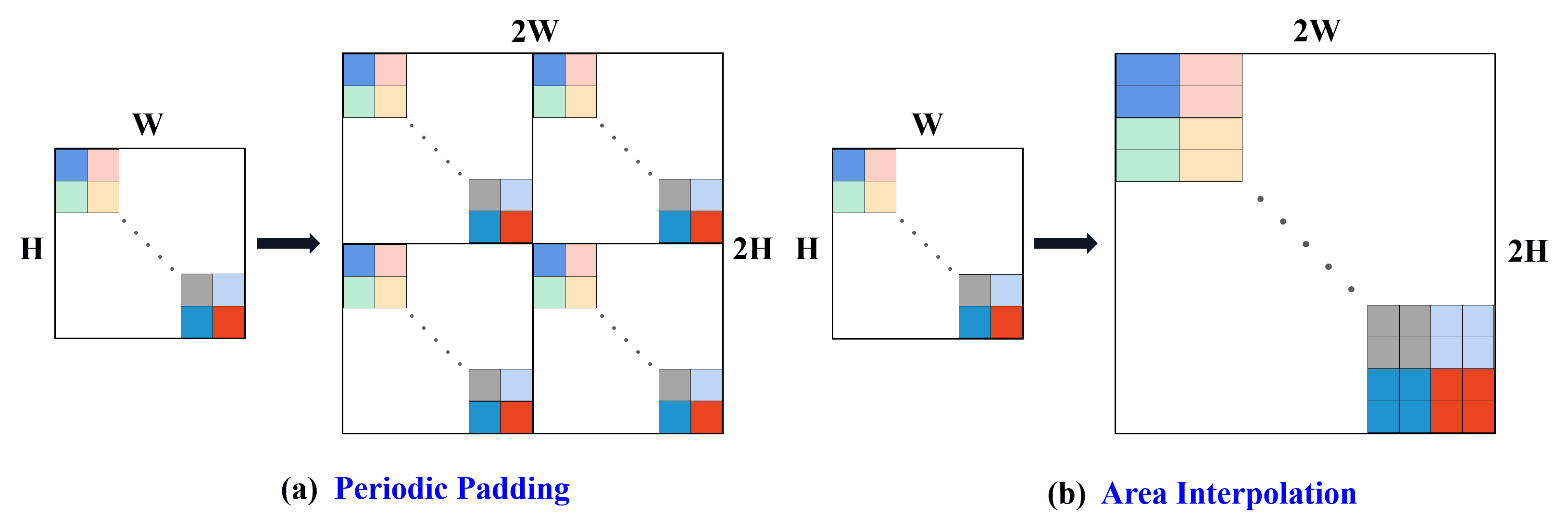
Figure 3: The illustrations of (a) periodic padding and (b) area interpolation in Figure 2. Each small color square represents a pixel of the amplitude/phase component in the Fourier domain.

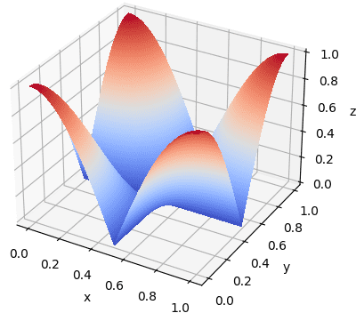
Figure 4: The surface of $A(x,y)$.

3.3 Architectural Design

Recall the Theorem-1 and Theorem-2, we propose two deep Fourier up-sampling variants: Periodic Padding and Area Interpolation-Cropping.

Periodic Padding Up-Sampling. The pseudo-code of Periodic Padding Up-Sampling is shown in the left of Figure 2. Given an image $\mathrm{X\in\mathbb{R}^{H\times W\times C}}$, we first adopt the Fourier transform $\mathrm{FFT(X)}$ to obtain its amplitude component $\mathrm{A}$ and phase component $\mathrm{P}$. We then perform the periodic padding over $\mathrm{A}$ and $\mathrm{P}$ two times in both the $H$ and $W$ dimensions, as illustrated in Figure 3(a). The padded $\mathrm{A\_pep}$ and $\mathrm{P\_pep}$ are then fed into two independent convolution module with $1\times 1$ kernel and followed by the inverse Fourier transform $\mathrm{iFFT(.)}$ to project the padded ones back to spatial domain.

Area Interpolation-Cropping Up-Sampling. The pseudo-code of Area interpolation-Cropping Up-Sampling is shown in the right of Figure 2. We first conduct the Area interpolation over the phase and amplitude by $2\times 2$ area interpolation with the same pixel, as illustrated in Figure 3(b). We then employ the inverse Fourier transform to project the interpolated ones back to spatial domain. As described in Section 3.2, the inverse spatial representation will be periodic while the pixel value will be decay. The degree of decay of the pixel increases when the pixel is closer to the center. To better maintain the information, we perform the area cropping operation (detailed in Figure 1) in the four corners with the $\frac{W}{2}\times\frac{H}{2}$ size and then merge them together as a whole at spatial dimension, finally resize them to the size of $2H\times 2W$.

Note that albeit being designed on the basis of strict theories, both constructed spectral up-sampling modules contain certain approximations, like a learnable $1\times 1$ convolution operator instead of strictly $1/4$ as described in Theorem-1 of main manuscript, and an approximation cropping to preserve the map corners instead of accurate $A$ mapping as proved in Theorem-2 of main manuscript and Theorem-3 of supplementary materials. Such strategy makes the proposed modules able to be more easily implemented and more flexibly represent real data spectral structures. It is worth noting that this should be the first attempt for constructing easy equitable spectral upsampling modules, and hope it would inspire more effective and rational ones from more spectral perspectives.

4 Experiments

To demonstrate the efficacy of our proposed deep Fourier up-sampling, we conduct extensive experiments on multiple computer vision tasks, including object detection, image segmentation, image de-raining, image dehazing, and guided image super-resolution. We provide more experimental results in the supplementary material.

4.1 Experimental Settings

Object Detection. Following [12], the PASCAL VOC 2007 and 2012 training sets [37] are used as training data. The PASCAL VOC 2007 testing set is used for evaluations as the ground truth annotations of VOC 2012 testing set are not publicly available. We employ the FPN-based Faster RCNN [12] with ResNet50 backbone and YOLO-v3 with Darknet53 [38] as baselines.

Image Segmentation. Following [39, 40], Synapse Dataset and CANDI Dataset are used as the testbed of medical image segmentation. We adopt the two representative image segmentation algorithms, U-Net [1] and Att-UNet [41], as the base models.

Image De-raining. Following [42], we choose two widely-used standard benchmark datasets, including Rain200H and Rain200L, for evaluations. we employ two representative de-raining methods, LPNet with up-sampling [11] and PReNet without up-sampling [42], as baselines.

Image Dehazing. Following [10], we employ RESIDE[43] dataset [44] for evaluations. We also use two different network designs AODNet [45] without up-sampling operator and MSBDN [10] with up-sampling operator, for validation.

Guided Image Super-resolution. Following [14, 46], we adopt the pan-sharpening, the representative task of guided image super-resolution, for evaluations. The WorldView II, WorldView III, and GaoFen2 in [14, 46] are used for evaluations. We employ two different network designs for validation, including PANNET [47] without up-sampling operator and DCFNET [48] with up-sampling operator.

Several widely-used image quality assessment (IQA) metrics are employed to evaluate the performance, including the relative dimensionless global error in synthesis (ERGAS) [49], the peak signal-to-noise ratio (PSNR), the spectral angle mapper (SAM) [50], DSC, and HD95.

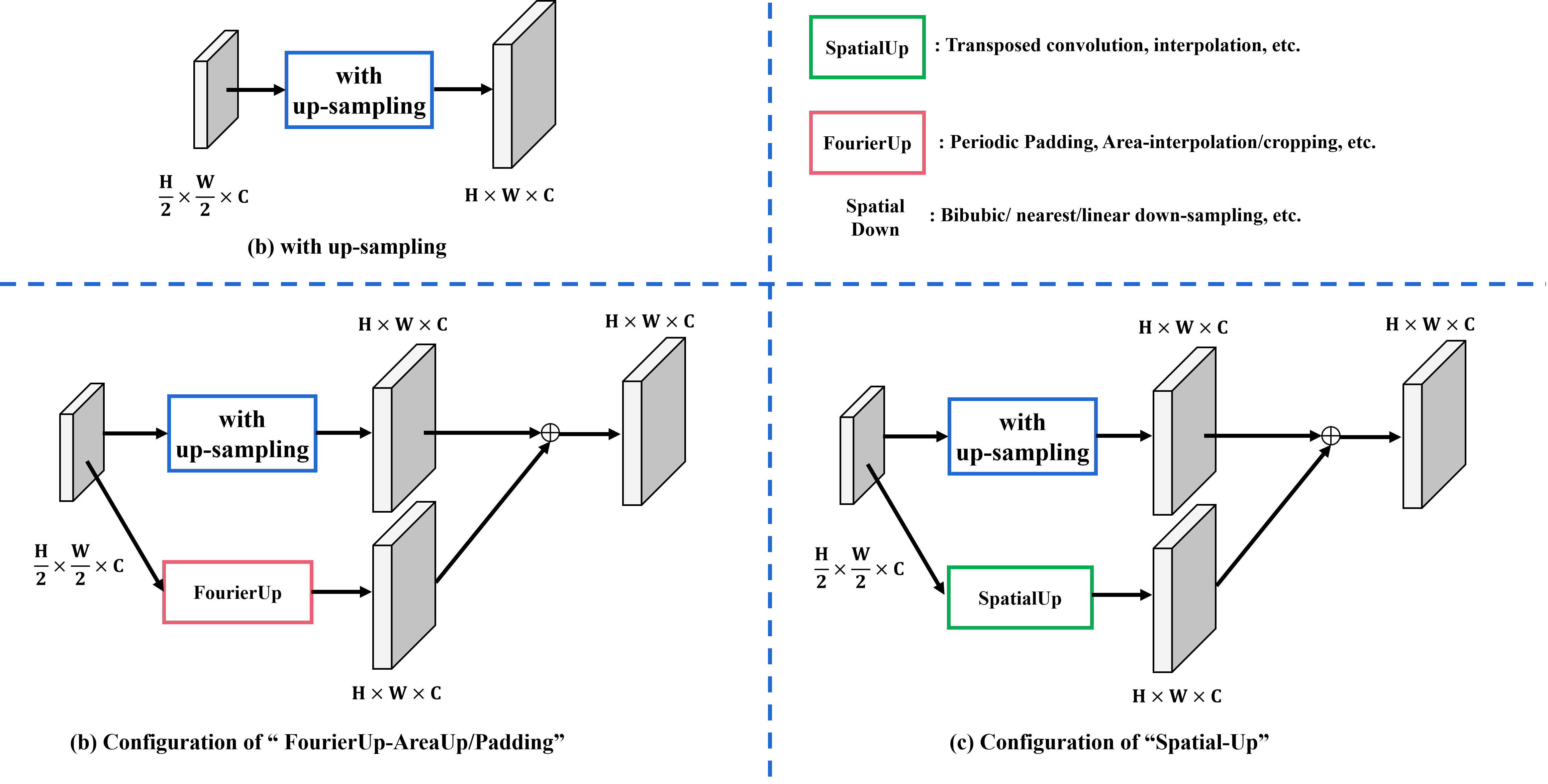
Figure 5: The implementation details of FourierUp into the existing baselines with up-sampling.

4.2 Implementation Details

Regarding the above competitive baselines, they can be divided into two categories: one with spatial up-sampling ([1], Att-UNet [41], DCFNET [48], LPNet [11], MSBDN [10]) and another one without spatial up-sampling (PReNet [42], AODNet[45], PANNET [47]). The purpose of the exploration on the baselines without spatial up-sampling is to show the versatility of our FourierUp for different network structures. Different from directly replacing the spatial up-sampling with the FourierUp in the baselines with spatial up-sampling, we need to encapsulate the FourierUp for the baselines without spatial up-sampling, in which a down-sampling operation is introduced to first reduce the resolution of features. We provide the detailed structures of the encapsulated FourierUp and the baselines with the FourierUp in the Figure 5 and supplementary material.

For the baselines with spatial up-sampling, we perform the comparison over four configurations:

• Original: the baseline without any changes;

• FourierUp-AreaUp: replacing the original model’s spatial up-sampling with the union of the Area-Interpolation variant of our FourierUp and the spatial up-sampling itself;

• FourierUp-Padding: replacing the original model’s spatial up-sampling operator with the union of the Periodic-Padding variant of our FourierUp and the spatial up-sampling itself;

• Spatial-Up: replacing the variants of FourierUp in the settings of $2)/3)$ with the spatial up-sampling. For a fair comparison, we use the same number of trainable parameters as $2)/3)$.

For the baselines without spatial up-sampling, we perform the comparison over four configurations:

• Original: the baseline without any changes;

• FourierUp-AreaUp: replacing the original model’s convolution with the encapsulated FourierUp that is equipped with the Area-Interpolation variant;

• FourierUp-Padding: replacing the original model’s convolution with the encapsulated FourierUp that is equipped with the Periodic-Padding variant;

• Spatial-Up: replacing the the encapsulated FourierUp of the settings of $2)/3)$ with the spatial up-sampling. For a fair comparison, we use the same number of trainable parameters as $2)/3)$.

4.3 Comparison and Analysis

Quantitative Comparison. We perform the model performance comparison over different configurations, as described in implementation details. The quantitative results are presented in Tables 1 to 3 where the best and second best results are highlighted in bold and Underline. From the results, by integrating with our proposed two FourierUp variants, we can observe performance gain against the baselines across all the datasets in all tested tasks, suggesting the effectiveness of our approach. For example, for the PReNet of Table 1, “FourierUp-padding” and “FourierUp-AreaUp” obtain 0.83dB/0.65dB and 2.1dB/1.9dB PSNR gains than the “Original”, 0.52dB/0.34dB and 1.7dB/1.5dB PSNR gains than “Spatial-Up” on the Rain200H and Rain200L datasets, respectively. Such results validate the effectiveness of our proposed FourierUp. The corresponding visualization consistently supports the analysis in Figure 6, where the FourierUp is capable of better maintaining the details.

Qualitative Comparison. Due to the limited space, we only report the visual results of the de-raining/dehazing task in Figures 6 and 7 that can more clearly show the effectiveness of FourierUp. More results can be found in the supplementary materials. As shown, integrating the FourierUp with the original baseline achieves more visually pleasing results. Specifically, zooming-in the red box region of Figures 6 and 7, the model equipped with the FourierUp is capable of better recovering the texture details while removing the rain/hazy effect.

Table 1: Quantitative comparisons of image de-raining.

Model	Configurations	Rain200H		Rain200L
		PSNR	SSIM	PSNR	SSIM
LPNet	Original	22.907	0.775	32.461	0.947
	Spatial-Up	22.956	0.777	32.522	0.950
	FourierUp-AreaUp	22.163	0.783	32.681	0.954
	FourierUp-Padding	23.295	0.786	32.835	0.956
PReNet	Original	29.041	0.891	37.802	0.981
	Spatial-Up	29.357	0.901	38.271	0.985
	FourierUp-AreaUp	29.690	0.903	39.776	0.985
	FourierUp-Padding	29.871	0.908	39.971	0.987

tableComparison over image dehazing. Model configurations PSNR SSIM AODNet Original 18.80 0.834 Spatial-Up 18.91 0.838 FourierUp-AreaUp 19.16 0.843 FourierUp-Padding 19.35 0.847 MSBDN Original 33.79 0.984 Spatial-Up 33.90 0.984 FourierUp-AreaUp 34.21 0.985 FourierUp-Padding 34.35 0.987

tableComparison over object detection. Model Methods AP50 mAP Faster RCNN Original 79.13 79.10 Spatial-Up 79.14 79.10 FourierUp-AreaUp 79.16 79.13 FourierUp-Padding 79.19 79.15 YOLO-V3 Original 81.68 81.63 Spatial-Up 81.68 81.63 FourierUp-AreaUp 81.70 81.65 FourierUp-Padding 81.72 81.68

Table 2: Quantitative comparisons of medical image segmentation.

Model	Configurations	synapse		CANDI
		DSC $\uparrow$	HD95 $\downarrow$	DSC $\uparrow$	HD95 $\downarrow$
U-Net	Original	76.85	39.70	86.50	3.946
	Spatial-Up	76.94	38.59	86.59	3.826
	FourierUp-AreaUp	77.25	36.02	86.63	3.751
	FourierUp-Padding	77.37	35.86	86.70	3.327
Att-UNet	Original	77.77	36.02	86.29	5.601
	Spatial-Up	77.85	35.91	86.35	5.588
	FourierUp-AreaUp	78.11	34.54	86.50	4.851
	FourierUp-Padding	78.34	34.29	86.64	4.833

Table 3: Quantitative comparisons of pan-sharpening.

Model	Configurations	WorldView-II				GaoFen2
		PSNR$\uparrow$	SSIM$\uparrow$	SAM$\downarrow$	ERGAS$\downarrow$	PSNR$\uparrow$	SSIM$\uparrow$	SAM$\downarrow$	EGAS$\downarrow$
PANNET	Original	40.817	0.963	0.025	1.055	43.066	0.968	0.018	0.855
	Spatial-Up	40.988	0.963	0.025	1.031	43.897	0.973	0.018	0.737
	FourierUp-AreaUp	41.167	0.963	0.024	1.010	45.964	0.979	0.015	0.653
	FourierUp-Padding	41.288	0.965	0.024	1.007	46.145	0.982	0.012	0.622
DCFNET	Original	40.276	0.968	0.028	1.051	42.986	0.967	0.019	0.858
	Spatial-Up	40.319	0.968	0.028	1.046	43.157	0.970	0.017	0.850
	FourierUp-AreaUp	40.484	0.968	0.025	1.115	43.881	0.979	0.014	0.829
	FourierUp-Padding	40.546	0.968	0.025	1.102	44.153	0.981	0.014	0.765

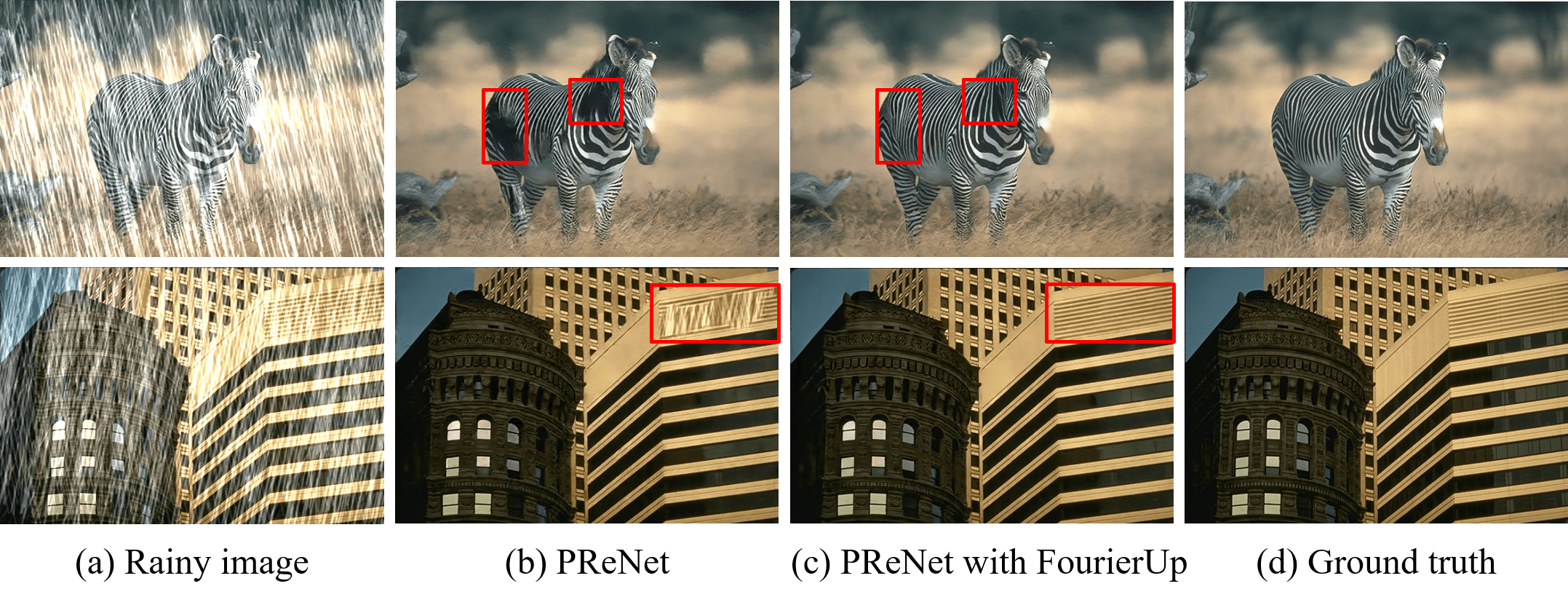
Figure 6: Visual comparison of PReNet on the Rain200H.

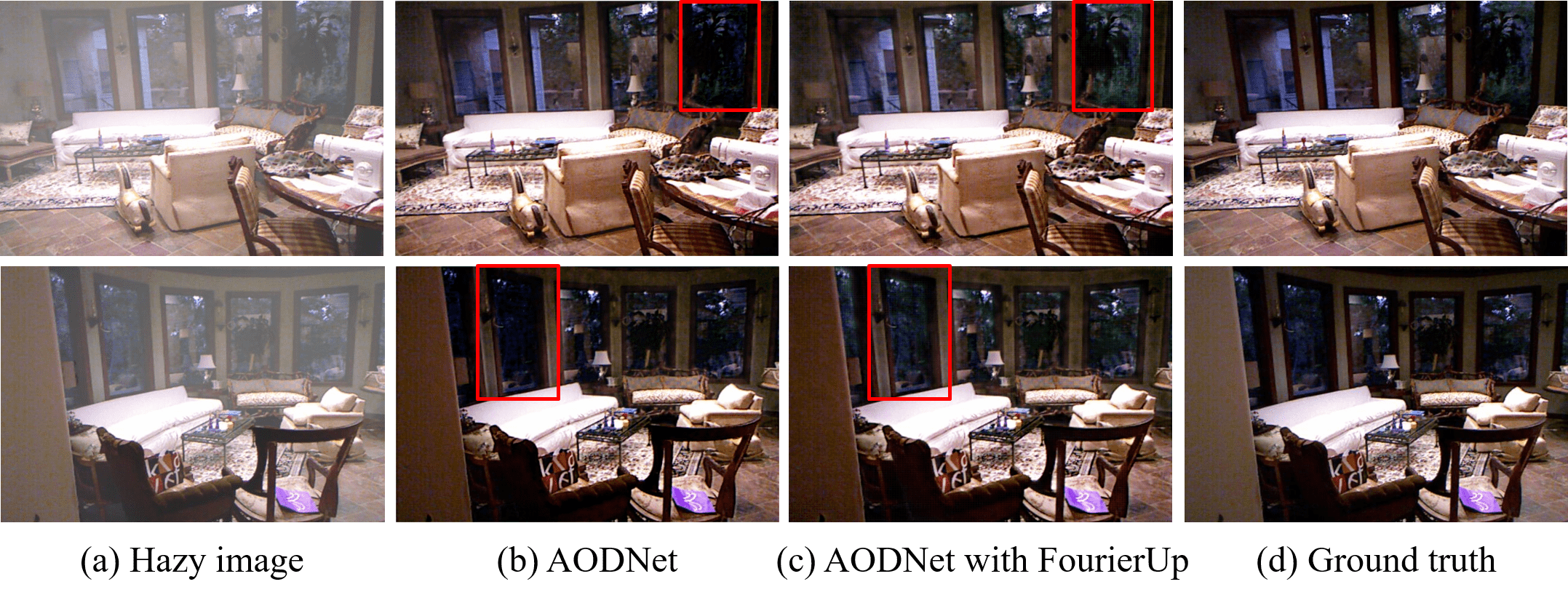
Figure 7: Visual comparison of AODNet on the SOTS.

5 Limitations

First, the more comprehensive experiments on broader computer vision tasks (e.g., image de-noising and image de-blurring) have not been explored. Second, the deep Fourier Up-sampling integrated with spatial up-sampling will increase the model parameter numbers. This is negligible at the significant performance gain at fewer parameter increase. Note that, the focus of this work is beyond designing a plug-and-play module to integrate it into existing networks for further performance gain. This work also provides a powerful scale change choice of the up-sampling operator pool when developing a new model from start.

6 Conclusion

In this paper, we have proposed a deep Fourier up-sampling to explore the possibility of the up-sampling in the Fourier domain, which provides the key insight for the multi-scale Fourier pattern modeling. We theoretically demonstrate that our designs of Fourier up-sampling are feasible. It is appealing that the proposed FourierUp is a generic operator, thus being directly integrated with existing networks. Extensive experiments demonstrate the effectiveness of our method. We believe the FourierUp has the potential to advance broader computer vision tasks, e.g., image/video super-resolution and image/video in-painting.

Broader Impact

Our work shows the promising capability of up-sampling in the Fourier domain for computer vision algorithms through two novel designs with theoretical proofs. Using our deep Fourier up-sampling with negligible computational cost will improve the performance of neural networks and facilitate the development of AI in real-world applications. However, the efficacy of our method may raise potential concerns when it is improperly used. For example, the safety of the applications of our method in real-world applications may not be guaranteed. We will investigate the robustness and effectiveness of our method in broader real-world applications.

References

Checklist

1. For all authors…

   1. Do the main claims made in the abstract and introduction accurately reflect the paper’s contributions and scope? [Yes]

   2. Did you describe the limitations of your work? [Yes] , see Section 5.

   3. Did you discuss any potential negative societal impacts of your work? [Yes] , see Section Broader Impact.

   4. Have you read the ethics review guidelines and ensured that your paper conforms to them? [Yes]

2. If you are including theoretical results…

   1. Did you state the full set of assumptions of all theoretical results? [Yes] , See Section 3.1 and Section 3.2.

   2. Did you include complete proofs of all theoretical results? [Yes] , See Section 3.1 and Section 3.2.

3. If you ran experiments…

   1. Did you include the code, data, and instructions needed to reproduce the main experimental results (either in the supplemental material or as a URL)? [Yes]

   2. Did you specify all the training details (e.g., data splits, hyperparameters, how they were chosen)? [Yes]

   3. Did you report error bars (e.g., with respect to the random seed after running experiments multiple times)? [No] , the effect of random seed could almost be negligible since we set the same initiation seed during experiments. Reproducibility can be guaranteed.

   4. Did you include the total amount of compute and the type of resources used (e.g., type of GPUs, internal cluster, or cloud provider)? [Yes]

4. If you are using existing assets (e.g., code, data, models) or curating/releasing new assets…

   1. If your work uses existing assets, did you cite the creators? [Yes]

   2. Did you mention the license of the assets? [Yes]

   3. Did you include any new assets either in the supplemental material or as a URL? [Yes]

   4. Did you discuss whether and how consent was obtained from people whose data you’re using/curating? [Yes] , the data creators claim that they allow and encourage the data for scientific research.

   5. Did you discuss whether the data you are using/curating contains personally identifiable information or offensive content? [N/A] , We train and test the framework using the publicly accessible datasets.

5. If you used crowdsourcing or conducted research with human subjects…

   1. Did you include the full text of instructions given to participants and screenshots, if applicable? [N/A]

   2. Did you describe any potential participant risks, with links to Institutional Review Board (IRB) approvals, if applicable? [N/A]

   3. Did you include the estimated hourly wage paid to participants and the total amount spent on participant compensation? [N/A]

References

- [1] Olaf Ronneberger, Philipp Fischer, and Thomas Brox. U-net: Convolutional networks for biomedical image segmentation. In International Conference on Medical image computing and computer-assisted intervention, pages 234–241. Springer, 2015.
- [2] Tsung-Yi Lin, Piotr Dollár, Ross Girshick, Kaiming He, Bharath Hariharan, and Serge Belongie. Feature pyramid networks for object detection. In Proceedings of the IEEE conference on computer vision and pattern recognition, pages 2117–2125, 2017.
- [3] Seung-Wook Kim, Hyong-Keun Kook, Jee-Young Sun, Mun-Cheon Kang, and Sung-Jea Ko. Parallel feature pyramid network for object detection. In Proceedings of the European Conference on Computer Vision (ECCV), pages 234–250, 2018.
- [4] Selim Seferbekov, Vladimir Iglovikov, Alexander Buslaev, and Alexey Shvets. Feature pyramid network for multi-class land segmentation. In Proceedings of the IEEE Conference on Computer Vision and Pattern Recognition Workshops, pages 272–275, 2018.
- [5] Lei Zhu, Zijun Deng, Xiaowei Hu, Chi-Wing Fu, Xuemiao Xu, Jing Qin, and Pheng-Ann Heng. Bidirectional feature pyramid network with recurrent attention residual modules for shadow detection. In Proceedings of the European Conference on Computer Vision (ECCV), pages 121–136, 2018.
- [6] Yanwei Pang, Tiancai Wang, Rao Muhammad Anwer, Fahad Shahbaz Khan, and Ling Shao. Efficient featurized image pyramid network for single shot detector. In Proceedings of the IEEE/CVF Conference on Computer Vision and Pattern Recognition, pages 7336–7344, 2019.
- [7] Ziming Liu, Guangyu Gao, Lin Sun, and Li Fang. Ipg-net: Image pyramid guidance network for small object detection. In Proceedings of the IEEE/CVF Conference on Computer Vision and Pattern Recognition Workshops, pages 1026–1027, 2020.
- [8] Edward H Adelson, Charles H Anderson, James R Bergen, Peter J Burt, and Joan M Ogden. Pyramid methods in image processing. RCA engineer, 29(6):33–41, 1984.
- [9] Jiapeng Luo, Jiaying Liu, Jun Lin, and Zhongfeng Wang. A lightweight face detector by integrating the convolutional neural network with the image pyramid. Pattern Recognition Letters, 133:180–187, 2020.
- [10] Hang Dong, Jinshan Pan, Lei Xiang, Zhe Hu, Xinyi Zhang, Fei Wang, and Ming-Hsuan Yang. Multi-scale boosted dehazing network with dense feature fusion. In 2020 IEEE/CVF Conference on Computer Vision and Pattern Recognition (CVPR), pages 2154–2164, 2020.
- [11] Xueyang Fu, Borong Liang, Yue Huang, Xinghao Ding, and John Paisley. Lightweight pyramid networks for image deraining. IEEE Transactions on Neural Networks and Learning Systems, 31(6):1794–1807, 2020.
- [12] Shaoqing Ren, Kaiming He, Ross Girshick, and Jian Sun. Faster r-cnn: Towards real-time object detection with region proposal networks. IEEE Transactions on Pattern Analysis and Machine Intelligence, 39(6):1137–1149, 2017.
- [13] Xueyang Fu, Zeyu Xiao, Gang Yang, Aiping Liu, Zhiwei Xiong, et al. Unfolding taylor’s approximations for image restoration. Advances in Neural Information Processing Systems, 34:18997–19009, 2021.
- [14] Man Zhou, Xueyang Fu, Jie Huang, Feng Zhao, Aiping Liu, and Rujing Wang. Effective pan-sharpening with transformer and invertible neural network. IEEE Transactions on Geoscience and Remote Sensing, 60:1–15, 2022.
- [15] Man Zhou, Jie Huang, Xueyang Fu, Feng Zhao, and Danfeng Hong. Effective pan-sharpening by multiscale invertible neural network and heterogeneous task distilling. IEEE Transactions on Geoscience and Remote Sensing, 60:1–14, 2022.
- [16] Man Zhou, Keyu Yan, Jie Huang, Zihe Yang, Xueyang Fu, and Feng Zhao. Mutual information-driven pan-sharpening. In Proceedings of the IEEE/CVF Conference on Computer Vision and Pattern Recognition (CVPR), pages 1798–1808, June 2022.
- [17] Man Zhou, Fan Wang, Xian Wei, Rujing Wang, and Xue Wang. Pid controller-inspired model design for single image de-raining. IEEE Transactions on Circuits and Systems II: Express Briefs, 69(4):2351–2355, 2022.
- [18] Man Zhou and Rujing Wang. Control theory-inspired model design for single image de-raining. IEEE Transactions on Circuits and Systems II: Express Briefs, 69(2):649–653, 2022.
- [19] Man Zhou, Jie Xiao, Yifan Chang, Xueyang Fu, Aiping Liu, Jinshan Pan, and Zheng-Jun Zha. Image de-raining via continual learning. In Proceedings of the IEEE/CVF Conference on Computer Vision and Pattern Recognition (CVPR), pages 4907–4916, June 2021.
- [20] Man Zhou, Keyu Yan, Jinshan Pan, Wenqi Ren, Qi Xie, and Xiangyong Cao. Memory-augmented deep unfolding network for guided image super-resolution, 2022.
- [21] Lu Chi, Borui Jiang, and Yadong Mu. Fast fourier convolution. In H. Larochelle, M. Ranzato, R. Hadsell, M. F. Balcan, and H. Lin, editors, Advances in Neural Information Processing Systems, 2020.
- [22] Xintian Mao, Yiming Liu, Wei Shen, Qingli Li, and Yan Wang. Deep residual fourier transformation for single image deblurring. arXiv preprint arXiv:2111.11745, 2021.
- [23] Yulun Zhang, Huan Wang, Can Qin, and Yun Fu. Aligned structured sparsity learning for efficient image super-resolution. Advances in Neural Information Processing Systems, 34, 2021.
- [24] Yulun Zhang, Kunpeng Li, Kai Li, Gan Sun, Yu Kong, and Yun Fu. Accurate and fast image denoising via attention guided scaling. IEEE Transactions on Image Processing, 30:6255–6265, 2021.
- [25] Yuchen Fan, Jiahui Yu, Yiqun Mei, Yulun Zhang, Yun Fu, Ding Liu, and Thomas S Huang. Neural sparse representation for image restoration. Advances in Neural Information Processing Systems, 33:15394–15404, 2020.
- [26] Wenqi Ren, Jiawei Zhang, Jinshan Pan, Sifei Liu, Jimmy Ren, Junping Du, Xiaochun Cao, and Ming-Hsuan Yang. Deblurring dynamic scenes via spatially varying recurrent neural networks. IEEE transactions on pattern analysis and machine intelligence, 2021.
- [27] Wenqi Ren, Jiawei Zhang, Lin Ma, Jinshan Pan, Xiaochun Cao, Wangmeng Zuo, Wei Liu, and Ming-Hsuan Yang. Deep non-blind deconvolution via generalized low-rank approximation. Advances in neural information processing systems, 31, 2018.
- [28] He Zhang and Vishal M Patel. Density-aware single image de-raining using a multi-stream dense network. In Proceedings of the IEEE conference on computer vision and pattern recognition, pages 695–704, 2018.
- [29] He Zhang, Vishwanath Sindagi, and Vishal M Patel. Image de-raining using a conditional generative adversarial network. IEEE transactions on circuits and systems for video technology, 30(11):3943–3956, 2019.
- [30] Jinshan Pan, Sifei Liu, Deqing Sun, Jiawei Zhang, Yang Liu, Jimmy Ren, Zechao Li, Jinhui Tang, Huchuan Lu, Yu-Wing Tai, et al. Learning dual convolutional neural networks for low-level vision. In Proceedings of the IEEE conference on computer vision and pattern recognition, pages 3070–3079, 2018.
- [31] Zongsheng Yue, Hongwei Yong, Qian Zhao, Deyu Meng, and Lei Zhang. Variational denoising network: Toward blind noise modeling and removal. In Advances in Neural Information Processing Systems, volume 32, 2019.
- [32] Yanchao Yang and Stefano Soatto. Fda: Fourier domain adaptation for semantic segmentation, 2020.
- [33] Shaohua Li, Kaiping Xue, Bin Zhu, Chenkai Ding, Xindi Gao, David Wei, and Tao Wan. Falcon: A fourier transform based approach for fast and secure convolutional neural network predictions. In Proceedings of the IEEE/CVF Conference on Computer Vision and Pattern Recognition, pages 8705–8714, 2020.
- [34] Jae-Han Lee, Minhyeok Heo, Kyung-Rae Kim, and Chang-Su Kim. Single-image depth estimation based on fourier domain analysis. In Proceedings of the IEEE Conference on Computer Vision and Pattern Recognition, pages 330–339, 2018.
- [35] Caiwen Ding, Siyu Liao, Yanzhi Wang, Zhe Li, Ning Liu, Youwei Zhuo, Chao Wang, Xuehai Qian, Yu Bai, Geng Yuan, et al. Circnn: accelerating and compressing deep neural networks using block-circulant weight matrices. In Proceedings of the 50th Annual IEEE/ACM International Symposium on Microarchitecture, pages 395–408, 2017.
- [36] Oren Rippel, Jasper Snoek, and Ryan P Adams. Spectral representations for convolutional neural networks. Advances in neural information processing systems, 28, 2015.
- [37] M. Everingham, L. V. Gool, Cki Williams, J. Winn, and A. Zisserman. The pascal visual object classes (voc) challenge. International Journal of Computer Vision, 88(2):303–338, 2010.
- [38] Mingxing Tan, Ruoming Pang, and Quoc V. Le. Efficientdet: Scalable and efficient object detection. In 2020 IEEE/CVF Conference on Computer Vision and Pattern Recognition (CVPR), pages 10778–10787, 2020.
- [39] Jieneng Chen, Yongyi Lu, Qihang Yu, Xiangde Luo, Ehsan Adeli, Yan Wang, Le Lu, Alan L Yuille, and Yuyin Zhou. Transunet: Transformers make strong encoders for medical image segmentation. arXiv preprint arXiv:2102.04306, 2021.
- [40] Shuhao Fu, Yongyi Lu, Yan Wang, Yuyin Zhou, Wei Shen, Elliot Fishman, and Alan Yuille. Domain adaptive relational reasoning for 3d multi-organ segmentation. In International Conference on Medical Image Computing and Computer-Assisted Intervention, pages 656–666. Springer, 2020.
- [41] Ozan Oktay, Jo Schlemper, Loic Le Folgoc, Matthew Lee, Mattias Heinrich, Kazunari Misawa, Kensaku Mori, Steven McDonagh, Nils Y Hammerla, Bernhard Kainz, et al. Attention u-net: Learning where to look for the pancreas. arXiv preprint arXiv:1804.03999, 2018.
- [42] Dongwei Ren, Wangmeng Zuo, Qinghua Hu, Pengfei Zhu, and Deyu Meng. Progressive image deraining networks: A better and simpler baseline. In Proceedings of the IEEE/CVF Conference on Computer Vision and Pattern Recognition (CVPR), June 2019.
- [43] Boyi Li, Wenqi Ren, Dengpan Fu, Dacheng Tao, Dan Feng, Wenjun Zeng, and Zhangyang Wang. Benchmarking single-image dehazing and beyond. IEEE Transactions on Image Processing, 28(1):492–505, 2019.
- [44] Yanfu Zhang, Li Ding, and Gaurav Sharma. Hazerd: An outdoor scene dataset and benchmark for single image dehazing. In 2017 IEEE International Conference on Image Processing (ICIP), pages 3205–3209, 2017.
- [45] Boyi Li, Xiulian Peng, Zhangyang Wang, Jizheng Xu, and Dan Feng. Aod-net: All-in-one dehazing network. In Proceedings of the IEEE International Conference on Computer Vision (ICCV), Oct 2017.
- [46] Keyu Yan, Man Zhou, Liu Liu, Chengjun Xie, and Danfeng Hong. When pansharpening meets graph convolution network and knowledge distillation. IEEE Transactions on Geoscience and Remote Sensing, 60:1–15, 2022.
- [47] Junfeng Yang, Xueyang Fu, Yuwen Hu, Yue Huang, Xinghao Ding, and John Paisley. Pannet: A deep network architecture for pan-sharpening. In IEEE International Conference on Computer Vision, pages 5449–5457, 2017.
- [48] Xiao Wu, Ting-Zhu Huang, Liang-Jian Deng, and Tian-Jing Zhang. Dynamic cross feature fusion for remote sensing pansharpening. In Proceedings of the IEEE/CVF International Conference on Computer Vision (ICCV), pages 14687–14696, October 2021.
- [49] L. Alparone, L. Wald, J. Chanussot, C. Thomas, P. Gamba, and L. M. Bruce. Comparison of pansharpening algorithms: Outcome of the 2006 grs-s data fusion contest. IEEE Transactions on Geoscience and Remote Sensing, 45(10):3012–3021, 2007.
- [50] A. F. Goetz J. R. H. Yuhas and J. M. Boardman. Discrimination among semi-arid landscape endmembers using the spectral angle mapper (sam) algorithm. Proc. Summaries Annu. JPL Airborne Geosci. Workshop, pages 147–149, 1992.