Anticipating the DART impact: Orbit estimation of Dimorphos using a simplified model

Abstract

We used the times of occultations and eclipses between the components of the 65803 Didymos binary system observed in its lightcurves from 2003-2021 to estimate the orbital parameters of Dimorphos relative to Didymos. We employed a weighted least-squares approach and a modified Keplerian orbit model in order to accommodate the effects from non-gravitational forces such as Binary YORP that could cause a linear change in mean motion over time. We estimate that the period of the mutual orbit at the epoch 2022 September 26.0 TDB, the day of the DART impact, is $11.9214869\pm 0.000028$ h ($1\sigma$) and that the mean motion of the orbit is changing at a rate of $(5.0\pm 1.0)\times 10^{-18}$ rad s^-2 $(1\sigma$). The formal $3\sigma$ uncertainty in orbital phase of Dimorphos during the planned Double Asteroid Redirection Test (DART) mission is $5.4^{\circ}$. Observations from July to September 2022, a few months to days prior to the DART impact, should provide modest improvements to the orbital phase uncertainty and reduce it to about $4.2^{\circ}$. These results, generated using a relatively simple model, are consistent with those generated using the more sophisticated model of Scheirich & Pravec (2022), which demonstrates the reliability of our method and adds confidence to these mission-critical results.

1 Introduction

The binary near-Earth asteroid (65803) Didymos is the target of NASA’s Double Asteroid Redirection Test (DART) mission, a test of the kinetic impactor approach to planetary defense (Cheng et al., 2016). The mission was launched on 2021 November 22 and the spacecraft will impact the satellite of Didymos, named Dimorphos, on 2022 September 26. The primary objective of the DART mission is to change the orbital period of Dimorphos and measure this change using ground-based observations (Rivkin et al., 2021). The DART spacecraft carried along with it a Light Italian Cubesat for Imaging of Asteroids (LICIA cube), built by the Italian Space Agency, for observations of the Didymos system during the DART impact (Dotto et al., 2021). Didymos is also the target of the European Space Agency’s proposed Hera mission, which will rendezvous several years after DART for post-impact characterization of the target (Michel et al., 2018).

Didymos was discovered in 1996 by the Spacewatch telescope at Kitt Peak (MPEC 1996-H02) and its binary nature was discovered in 2003 November by Pravec et al. (2003) when mutual events (occultations/eclipses) were observed in lightcurves. The presence of a satellite was confirmed later that month when Arecibo radar images resolved echoes from the two objects (Naidu et al., 2020b). Naidu et al. used the radar and lightcurve data from 2003 to characterize the physical properties of the system, including a 3D shape model of the primary, size of the secondary, and mutual orbit parameters. The primary and secondary components are roughly 780 m and 150 m in diameter, respectively, and the mutual orbit of the system has a semimajor axis of $\sim 1.2$ km and a period of about 11.9 h (Pravec et al., 2006; Naidu et al., 2020b).

In order to characterize the pre-impact orbit of Dimorphos,  Pravec et al. (2022) obtained lightcurves of the system in 2015, 2017, 2019, 2020, and 2021 in addition to the original lightcurves from 2003 (Pravec et al., 2006). Scheirich & Pravec (2022) use the primary-subtracted lightcurves (where the primary lightcurve has been modeled and subtracted from the total lightcurve) to fit a binary asteroid model, including the mutual orbit parameters. They model the binary system as two ellipsoids orbiting each other on a modified Keplerian orbit. They use ray-tracing code and photometric models such as Lommel-Seeliger and Lambert scattering laws to model the orbital lightcurves. Similar methods were used to model orbits of other binary asteroids (e.g. Scheirich & Pravec, 2009).

In this paper we develop a simpler approach to estimate the mutual orbit parameters of the system by using only the times of the beginnings and ends of mutual events. This approach differs from that of Scheirich & Pravec (2022) in that it uses a different observational data type and different observational model. Our simplified approach allows us to determine the orbital parameters quickly compared to the approach of Scheirich & Pravec (2022) and our method is robust as demonstrated by the consistency of the results with those of Scheirich & Pravec (2022).

2 Observations

We used lightcurves from Pravec et al. (2006) and Pravec et al. (2022) and measured the times of mutual events detected in the orbital component of the lightcurves of Didymos. The decomposition of the total lightcurve into the primary and the primary-subtracted components was done by Pravec et al. (2006) for the 2003 data, by Pravec et al. (2022) for the 2015, 2017, and 2019 data, and by one of us (NM) for the 2020 and 2021 data. We used the Scheirich & Pravec (2022) model to determine the types of events. We could have determined the types of events without using the Scheirich & Pravec (2022) model, but it would have involved trial and error and involved additional effort. There are four different kinds of mutual events in the data: eclipse of the primary (secondary casting shadows on the primary), eclipse of the secondary, occultation of the primary from the point of view of the observer, and occultation of the secondary.

A mutual event causes a drop in the brightness of the system and typically has four contact times: the first contact is when the event begins and the brightness starts decreasing, the second contact is when the brightness reaches a minimum, the third contact is when the brightness starts increasing again, and the fourth contact is when the event ends and the brightness of the system returns to the baseline value. We use $T_{1}$, $T_{2}$, $T_{3}$, and $T_{4}$ to refer to these contact times. If the Sun-asteroid-observer phase angle is low, an eclipse and an occultation might overlap such that the event could begin as an eclipse/occultation and end as an occultation/eclipse. In some cases we might have partial events in which only a fraction of the primary and secondary undergo a mutual event. Overlapping events have ill-defined $T_{2}$ and $T_{3}$ whereas partial events lack $T_{2}$ and $T_{3}$. Complete secondary events have consistent depths because the entire contribution from the secondary vanishes, whereas the depths of complete primary events vary because the brightness of the primary varies across its surface. We neglect possible albedo variations on the primary, as well as phase effects at higher phase angles, both of which can affect the apparent local surface brightness of the primary. These assumptions imply that the primary event depths match the secondary event depths. We measured event times $T_{1.5}$ and $T_{3.5}$ (for both primary and secondary events) as the times when the drop in brightness of the system was half of the total drop in brightness due to a full secondary event. For a typical non-overlapping and complete event $T_{1.5}$ lies between $T_{1}$ and $T_{2}$, and $T_{3.5}$ lies between $T_{3}$ and $T_{4}$. We used $T_{1.5}$ and $T_{3.5}$ as our observations for the orbit determination.

For the Didymos system, with a diameter ratio (secondary/primary) of 0.21, a full secondary event causes a drop in brightness of 4.2% (Pravec et al., 2006). We measured $T_{1.5}$ and $T_{3.5}$ as the times when the brightness drops by 2.1%, which corresponds to a magnitude increase of 0.023. When the Sun-target-observer phase angle is zero, $T_{1.5}$ and $T_{3.5}$ correspond to start and end times of when the center-of-mass of the satellite undergoes a mutual event. Figure 1 shows the contact times for a secondary eclipse event from 2003. We used the average magnitude of the points adjacent to the event as the baseline magnitude of the lightcurve outside each event and plotted a horizontal line 0.023 magnitude above this baseline. We made measurements visually by inspecting the intersection of this line with the mutual events. We assigned $1\sigma$ uncertainties of $(T_{1.5}-T_{1})/2$ and $(T_{4}-T_{3.5})/2$ to $T_{1.5}$ and $T_{3.5}$, respectively. The assigned uncertainties take into account measurement errors as well as errors and variations in the assumed event depths. Table LABEL:tab:observations lists all the observations.

Table 1: Mutual event times measured in observations from 2003 to 2021. All times are one-way light-time corrected to reflect the time of the events at the asteroid, not the times that they were observed from Earth. The last column shows the residuals (observed - computed) for solution 104, which is described in Section 5

			Occulted/Eclipsed		$1\sigma$ Uncertainty	Residuals
Calendar date (UTC)	Julian date	Contact	object	Event type	(days)	(sigmas)
2003 Nov 20 22:48:00	2452964.4500	1.5	Secondary	Eclipse	0.004	0.7177
2003 Nov 21 00:01:26	2452964.5010	3.5	Secondary	Eclipse	0.004	-0.5260
2003 Nov 21 22:31:00	2452965.4382	1.5	Secondary	Eclipse	0.005	-0.1701
2003 Nov 21 23:52:30	2452965.4948	3.5	Secondary	Eclipse	0.011	-0.0028
2003 Nov 22 04:32:35	2452965.6893	1.5	Primary	Eclipse	0.004	0.5784
2003 Nov 22 05:50:21	2452965.7433	3.5	Primary	Eclipse	0.004	0.1697
2003 Nov 23 04:19:46	2452966.6804	1.5	Primary	Eclipse	0.004	0.3414
2003 Nov 23 05:38:49	2452966.7353	3.5	Primary	Eclipse	0.003	0.2542
2003 Nov 24 04:03:12	2452967.6689	1.5	Primary	Eclipse	0.003	-0.7358
2003 Nov 24 05:26:52	2452967.7270	3.5	Primary	Eclipse	0.006	0.0447
2003 Nov 26 03:40:36	2452969.6532	1.5	Primary	Eclipse	0.004	-0.5276
2003 Nov 26 05:03:33	2452969.7108	3.5	Primary	Eclipse	0.003	-0.0019
2003 Nov 27 21:27:12	2452971.3939	1.5	Secondary	Eclipse	0.005	0.4601
2003 Nov 29 21:01:17	2452973.3759	1.5	Secondary	Eclipse	0.003	0.0022
2003 Nov 30 02:57:33	2452973.6233	1.5	Primary	Eclipse	0.003	-0.1950
2003 Dec 02 03:55:35	2452975.6636	3.5	Primary	Occultation	0.005	-0.3090
2003 Dec 03 03:38:44	2452976.6519	3.5	Primary	Occultation	0.011	-0.4991
2003 Dec 03 08:16:13	2452976.8446	1.5	Secondary	Eclipse	0.006	-0.6084
2003 Dec 03 09:46:22	2452976.9072	3.5	Secondary	Occultation	0.009	0.1859
2003 Dec 04 02:17:31	2452977.5955	1.5	Primary	Eclipse	0.004	0.6318
2003 Dec 04 03:35:59	2452977.6500	3.5	Primary	Occultation	0.004	0.0754
2003 Dec 18 23:29:19	2452992.4787	1.5	Primary	Eclipse	0.013	0.0933
2003 Dec 19 00:50:58	2452992.5354	3.5	Primary	Occultation	0.009	-0.2509
2003 Dec 19 05:23:16	2452992.7245	1.5	Secondary	Eclipse	0.009	-0.1319
2003 Dec 19 06:44:55	2452992.7812	3.5	Secondary	Occultation	0.008	-0.6452
2003 Dec 20 05:19:06	2452993.7216	1.5	Secondary	Eclipse	0.004	0.8909
2003 Dec 20 06:32:15	2452993.7724	3.5	Secondary	Occultation	0.008	-0.8477
2015 Apr 13 04:54:20	2457125.7044	3.5	Primary	Occultation	0.007	0.0336
2015 Apr 14 09:25:37	2457126.8928	1.5	Secondary	Eclipse	0.004	-0.6243
2017 Feb 25 03:50:06	2457809.6598	1.5	Primary	Occultation	0.005	-0.3512
2017 Feb 25 05:45:10	2457809.7397	3.5	Primary	Eclipse	0.006	1.6079
2017 Apr 18 07:46:16	2457861.8238	1.5	Primary	Eclipse	0.004	0.0144
2017 May 04 06:49:32	2457877.7844	3.5	Primary	Occultation	0.005	0.3233
2019 Jan 31 08:39:24	2458514.8607	3.5	Secondary	Eclipse	0.007	-0.5171
2019 Jan 31 13:03:21	2458515.0440	1.5	Primary	Occultation	0.004	0.6895
2019 Mar 09 01:42:31	2458551.5712	1.5	Secondary	Occultation	0.007	0.4536
2019 Mar 09 02:35:13	2458551.6078	3.5	Secondary	Eclipse	0.005	-0.0914
2019 Mar 10 02:15:47	2458552.5943	3.5	Secondary	Eclipse	0.005	-1.2862
2019 Mar 11 02:15:30	2458553.5941	3.5	Secondary	Eclipse	0.005	-0.0786
2020 Dec 12 14:21:50	2459196.0985	1.5	Primary	Occultation	0.004	0.9640
2020 Dec 12 15:00:34	2459196.1254	3.5	Primary	Occultation	0.004	0.1897
2020 Dec 17 08:50:38	2459200.8685	1.5	Secondary	Eclipse	0.006	0.8257
2020 Dec 17 09:36:43	2459200.9005	3.5	Secondary	Eclipse	0.006	-0.3763
2020 Dec 23 08:32:55	2459206.8562	3.5	Secondary	Eclipse	0.007	-0.3514
2020 Dec 23 12:35:42	2459207.0248	1.5	Primary	Occultation	0.006	1.0714
2020 Dec 23 13:04:47	2459207.0450	3.5	Primary	Occultation	0.007	-0.3992
2021 Jan 08 10:57:12	2459222.9564	1.5	Primary	Eclipse	0.005	0.4413
2021 Jan 08 11:35:39	2459222.9831	3.5	Primary	Eclipse	0.006	-0.7766
2021 Jan 09 10:50:26	2459223.9517	1.5	Primary	Eclipse	0.010	0.4727
2021 Jan 09 11:21:15	2459223.9731	3.5	Primary	Eclipse	0.010	-0.7482
2021 Jan 10 11:11:02	2459224.9660	3.5	Primary	Eclipse	0.007	-1.0587
2021 Jan 12 15:06:46	2459227.1297	1.5	Secondary	Occultation	0.013	-0.1800
2021 Jan 14 09:56:44	2459228.9144	1.5	Primary	Eclipse	0.004	0.7749
2021 Jan 14 10:26:41	2459228.9352	3.5	Primary	Eclipse	0.009	-1.0657
2021 Jan 17 14:26:00	2459232.1014	1.5	Secondary	Occultation	0.007	-0.0537
2021 Jan 18 08:22:50	2459232.8492	1.5	Primary	Occultation	0.011	-0.0715
2021 Jan 18 09:00:17	2459232.8752	3.5	Primary	Occultation	0.007	0.1228
2021 Jan 18 09:14:41	2459232.8852	1.5	Primary	Eclipse	0.007	0.4403
2021 Jan 18 09:40:45	2459232.9033	3.5	Primary	Eclipse	0.017	-0.7859
2021 Jan 20 01:54:20	2459234.5794	1.5	Secondary	Occultation	0.006	-1.2584
2021 Jan 20 03:40:19	2459234.6530	3.5	Secondary	Eclipse	0.011	-0.1952

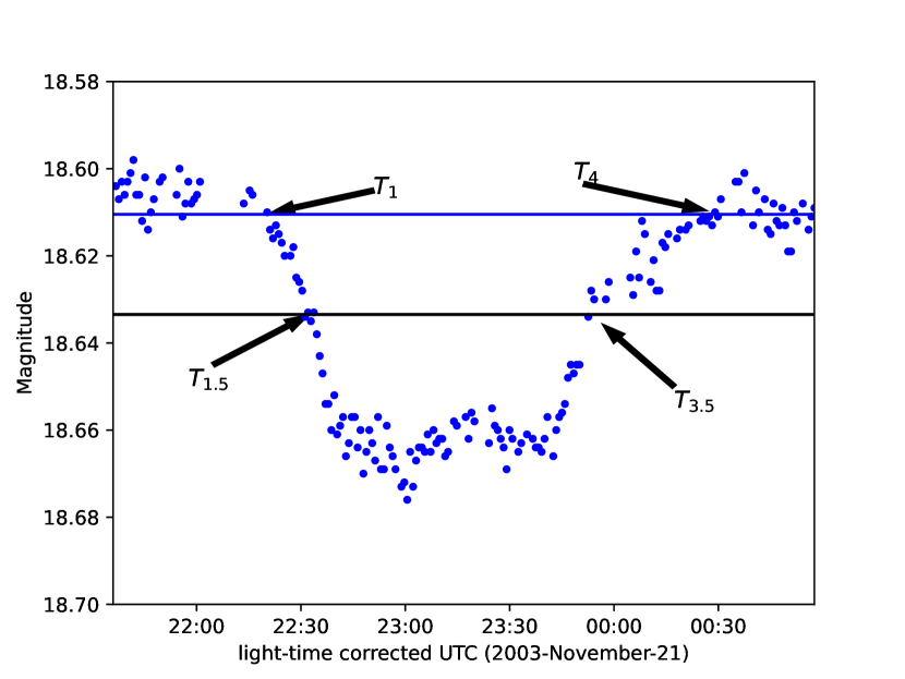
Figure 1: A secondary eclipse event showing various contact times. The horizontal blue line represents the baseline magnitude of the system and is computed by taking the average magnitude of the points just outside the mutual event. The black line indicates a magnitude that is fainter than the baseline by 0.023 mag, which represents a 2.1% drop in brightness of the system.

In addition to lightcurve mutual events, radar range and Doppler measurements of Dimorphos relative to Didymos were also available from Table 6 of Naidu et al. (2020b). We did not include these in the final orbit fit because they only span a short period in 2003 and do not provide any significant constraints to the orbital uncertainties during the DART impact in 2022 September. However, we used the radar measurements to check for consistency with the best-fit orbit by generating range and Doppler predictions at the time of the observations.

3 Orbit fit

We used a weighted least-squares method to estimate the best-fit model parameters (Milani & Gronchi, 2009). The goal is to minimize the cost function, $\chi^{2}=\boldsymbol{\nu}^{T}W\boldsymbol{\nu}$, where $\boldsymbol{\nu}$ is the array of residuals (observed - computed) and $W$ is the weight matrix with $W_{i,j}=0$ for $i\neq j$, and $W_{i,j}=1/\sigma_{i}^{2}$ for $i=j$, and $\sigma_{i}$ is the observational uncertainty for the $i$th observation.

The least-squares solution is found by iteratively correcting the estimated parameters $\boldsymbol{x}$ by

$$\Delta\boldsymbol{x}=-\Gamma B^{T}W\boldsymbol{\nu},$$ (1)

where $B=\partial\boldsymbol{\nu}/\partial x$ is the design matrix, $\Gamma=C^{-1}$ is the covariance matrix, and $C=B^{T}WB$ is the normal matrix, also called the information matrix. This iterative procedure is called differential corrections. The marginal $1\sigma$ uncertainties of the parameters are computed by taking the square root of the diagonal elements of the covariance matrix.

In order to compute $\boldsymbol{\nu}$, we have to use a model to calculate the “computed” value corresponding to each observation. We used the NAIF SPICE geometry finder tools (Acton et al., 2018) for this purpose. This calculation requires SPICE kernels that describe the trajectory, size, shape, and orientation of the objects. We modeled the primary as an oblate spheroid with dimensions of 830 x 830 x 786 m (Naidu et al., 2020b) with its spin pole aligned with the mutual orbit pole. This information is defined in a planetary constants kernel (PCK) file. The primary was treated as an ellipsoid for computing the mutual event timings but was treated as a point mass for computing its gravitational force on the satellite.

We assumed the satellite to be a point mass on a modified Keplerian mutual orbit around the primary. In addition to Keplerian motion, we included an additional term for modeling the drift in mean motion due to Binary YORP (BYORP, Ćuk, 2007). Assuming that the system mass is constant, a drift in mean motion leads to a change in semimajor axis with time. The mean anomaly ($M$) and mean motion ($n$) of the satellite at time $t$ are given by:

$$M(t)=M_{0}+n_{0}(t-t_{0})+\frac{1}{2}\dot{n}(t-t_{0})^{2},$$ (2)

$$n(t)=n_{0}+\dot{n}(t-t_{0}),$$

where $M_{0}$ and $n_{0}$ are the mean anomaly and mean motion of the satellite at time $t_{0}$, and $\dot{n}$ is the constant rate of change of mean motion due to BYORP (Ćuk, 2007). We used these equations to generate the states of the satellite with respect to the primary at 1-day intervals and saved them as SPK files. We used type-5 SPKs, which assume Keplerian motion for interpolating states. The time interval between states is small enough that errors in mean motion due to BYORP are orders of magnitude smaller than the uncertainty. Tests with 0.001 day intervals yield almost identical results.

To calculate the computed event times, we first computed time intervals for mutual events assuming a point-sized satellite. When the Sun-target-observer phase angle is zero, these times would correspond to the observed times, $T_{1.5}$ and $T_{3.5}$. However, at non-zero phase angles, eclipses and occultations are observable in the lightcurves for shorter durations: eclipses are observable only when a shadow is cast on the part of the target’s surface that is visible from Earth, while occultations are observable only when the sunlit part of the target’s surface is occulted. We took these phase effects into account in the following way.

For primary events, we computed the point on the surface of the primary that is being eclipsed or occulted by the secondary, which is assumed to be a point. We then use the SPICE geometry finder (Acton et al., 2018) to calculate intervals when the eclipsed point is visible from the Earth or when this occulted point is sunlit. The beginnings and ends of these intervals are taken to be the computed values of $T_{1.5}$ and $T_{3.5}$. Appropriate light-time corrections were made using the SPICE routines (Acton et al., 2018) so that the calculated event times correspond to the times at the asteroid, which is the timescale used in the observed lightcurves.

There are similar phase effects for secondary events. The dark part of the surface of the secondary does not contribute to the lightcurves. The only portion of the secondary surface that contributes to the lightcurves is the area that is sunlit and oriented towards Earth. So, for secondary events, the measured $T_{1.5}$ represents the instant when half of this visible area goes into an eclipse/occultation and $T_{3.5}$ represents the instant when half of the visible area comes out of an eclipse/occultation. We corrected the zero-phase mutual event times by computing the separation between the center of figure and the center of the visible area of the secondary and multiplying this separation by the relative velocity of the secondary in the direction of the separation.

For calculating the “computed” values of radar range separations, we used SPICE to subtract the distance of Didymos relative to Earth from the distance of Dimorphos relative to Earth. For calculating Doppler separations ($\Delta f$) we computed the magnitude of the velocity of Dimorphos relative to Didymos in the direction of Earth ($\Delta v$). Then Doppler separation was computed as:

$$\Delta f=2\frac{\Delta v}{c}F$$ (3)

where $c$ is the speed of light, $F$ is the frequency of radar waves (8560 MHz for Goldstone and 2380 MHz for Arecibo). The factor of two exists due to the fact that the radar signal gets Doppler shifted twice, once during transmission and once during reception (Ostro, 1993).

The design matrix, $\partial\boldsymbol{\nu}/\partial x$, was computed numerically using second order central differences:

$$\frac{\partial\boldsymbol{\nu}}{\partial P}=\frac{-\boldsymbol{\nu}(P+2\delta P)+8\boldsymbol{\nu}(P+\delta P)-8\boldsymbol{\nu}(P-\delta P)+\boldsymbol{\nu}(P-2\delta P)}{12\delta P},$$ (4)

where $\delta P$ is a small increment in the value of the parameter, $P$. The values for $\delta P$ were carefully chosen by numerically testing the values of the partials. For $M_{0}$, $n_{0}$, and $\dot{n}$ the increments were 0.01 rad, $10^{-10}$ rad s^-1, and $5\times 10^{-18}$ rad s^-2.

Our estimable parameters were $M_{0}$, $n_{0}$, and $\dot{n}$, whereas the remaining orbital parameters were fixed. The semimajor axis and eccentricity were set to 1.2 km and 0 respectively, based on estimates from Pravec et al. (2006) and Naidu et al. (2020b). The orbit pole longitude and latitude with respect to the IAU76 ecliptic frame (Seidelmann, 1977) were set to $320.6^{\circ}$ and $-78.6^{\circ}$ respectively, based on Scheirich & Pravec (2022). These correspond to a longitude of ascending node of $50.6^{\circ}$ and inclination of $168.6^{\circ}$. Given the zero eccentricity, we set the argument of pericenter to zero so that the mean anomaly is measured from the ascending node.

We used an initial value for $n_{0}$ corresponding to a $11.9216$ h orbital period based on the estimate from Scheirich and Pravec (personal communication). We set the initial value of $\dot{n}$ to 0 and for $M_{0}$, we tried initial values from $0^{\circ}$ to $350^{\circ}$ with a step size of $10^{\circ}$.

4 Predictions

The nominal values of $M$, $n$, and $\dot{n}$ are propagated to a time $t$ using equations 2. The covariance matrix is mapped to a different epoch using Milani & Gronchi (2009):

$$\Gamma_{t}=S\Gamma_{0}S^{T}$$ (5)

where

$$S=\frac{\partial(M_{t},n_{t},\dot{n})}{\partial(M_{0},n_{0},\dot{n})}=\begin{bmatrix}1&(t-t_{0})&\frac{1}{2}(t-t_{0})^{2}\\ 0&1&(t-t_{0})\\ 0&0&1\\ \end{bmatrix}$$

Here subscripts $t$ and $0$ denote parameters at time $t$ and $t_{0}$ respectively. The marginal $1\sigma$ uncertainties on the parameters are the square roots of the corresponding diagonal elements of $\Gamma_{t}$. The uncertainty on $\dot{n}$ does not change with time.

Similarly, predictions of observable uncertainties at time $t$ are computed as:

$$\Gamma_{T_{*}}=Q\Gamma_{t}Q^{T},$$ (6)

where

$$Q=\frac{\partial T_{*}}{\partial(M_{t},n_{t},\dot{n})}.$$ (7)

Here $T_{*}$ is the observed event time and $Q$ is computed numerically using second order central differences.

5 Results

The orbit fits starting from various initial values of $M_{0}$ converged to a single clear best-fit solution. Table 2 shows the best-fit parameters and formal $1\sigma$ uncertainties, and Table 3 shows the corresponding covariance. Residuals are given in Table LABEL:tab:observations. The value of $\chi^{2}_{\nu}$ and the residuals suggest that the assigned measurement uncertainties are conservative. The estimates from Table 2 are consistent with those from Scheirich & Pravec (2022) to well within $1\sigma$. We refer to this solution as 104. We also generated a separate solution by estimating all the mutual orbit parameters, which yielded an orbit pole of $(\lambda,\beta)=(310\pm 15,-76\pm 4)^{\circ}$ ($3\sigma$ uncertainties). This is consistent with the estimate of $(\lambda,\beta)=(320.6\pm 13.7,-78.6\pm 1.8)^{\circ}$ from Scheirich & Pravec (2022). For our final solution, 104, we decided to adopt the pole estimate of Scheirich & Pravec (2022) because it is more precise. Figure 2 compares projections of best-fit parameters and corresponding formal $3\sigma$ uncertainties of solution 104 with solutions having shorter data-arcs, 2003-2019, and 2003-2020. Each successive solution has smaller uncertainties and they are completely contained within the uncertainties of previous solutions, indicating that the three solutions are consistent and able to predict future solutions.

The formal $3\sigma$ uncertainty in the orbital phase of solution 104 during the planned DART impact date of 2022 September 26 is $5.4^{\circ}$. The formal uncertainties are underestimated because they do not take into account variations due to the sizes of the primary and secondary, orbit pole, eccentricity, argument of pericenter, and the obliquity of the orbit pole with respect to the spin pole of the primary. Naidu et al. (2020a) recommended that the formal uncertainties derived from the covariance matrix be multiplied by a factor of 1.3 to capture possible systematic errors due to unestimated parameters. Comparing the uncertainties with those from Scheirich & Pravec (2022) suggests that the formal uncertainties in Table 2 might be underestimated by up to a factor of 3.

Table 2: Best-fit orbital parameters of solution 104. The solution epoch was chosen to be JD 2455873.0 UTC for easy comparison with Scheirich & Pravec (2022). $M_{0}$, $n_{0}$ and $\dot{n}$ were estimated. Pole ($\lambda,\beta$) is not estimated and is taken from  Scheirich & Pravec (2022). The osculating period is derived from $n_{0}$. $GM_{sys}$ is the standard gravitational parameter of the system and is derived from the estimated value of $n_{0}$ and the assumed value of the semimajor axis at epoch. $\chi^{2}_{\nu}=\chi^{2}/(n_{obs}-n_{est})$ is the reduced $\chi^{2}$, where $n_{obs}$ is the number of observations and $n_{est}$ is the number of estimated parameters.

Parameter	Value $\pm~{}1\sigma$
$M_{0}$ (∘)	89.2 $\pm$ 1.8
Period (h)	11.9216262 $\pm$ 0.0000027
$n_{0}$ (rad s-1)	$(1.46400266\pm 0.00000035)\times 10^{-4}$
$\dot{n}$ (rad s-2)	$(5.0\pm 1.0)\times 10^{-18}$
Epoch (UTC)	2011-11-07 12:00:00
$\chi^{2}$	21.6
$\chi^{2}_{\nu}$	0.37
$(\lambda,\beta)^{\circ}$	$(320.6,-78.6)^{\circ}$
$GM_{sys}$ (m3 s-2)	37.03627274882414

Table 3: Covariance matrix corresponding to solution 104 in Table 2 at epoch 2011-11-07 12:00:00 UTC. Units of the parameters are in radians and seconds.

	$M_{0}$	$n_{0}$	$\dot{n}$
$M_{0}$	$1.03789679\times 10^{-03}$	$1.65661906\times 10^{-13}$	$-3.10150235\times 10^{-20}$
$n_{0}$	$1.65661906\times 10^{-13}$	$1.13162377\times 10^{-21}$	$-3.31164606\times 10^{-30}$
$\dot{n}$	$-3.10150235\times 10^{-20}$	$-3.31164606\times 10^{-30}$	$9.93383023\times 10^{-37}$

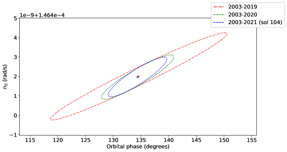
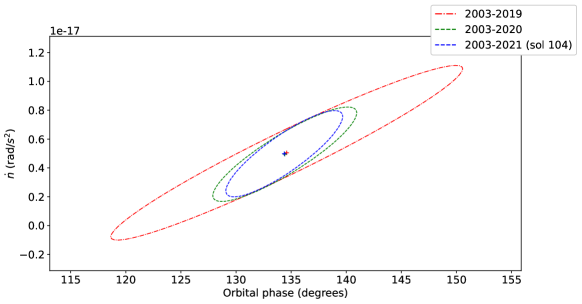
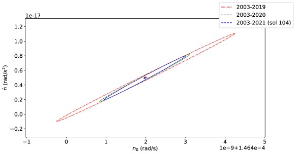
Figure 2: Projections of the best-fit parameters and their $3\sigma$ uncertainties for various orbital solutions of Dimorphos. The solution using a data-arc of 2003-2019 is shown in red and the solution using a data-arc of 2003-2020 is shown in green. Solution 104, the current best-fit solution, is shown in blue. Solutions are mapped to epoch 2022-Sep-26 23:15 UTC, the DART impact time. Orbital phase is the angle in the orbital plane measured from the $0^{\circ}$ longitude in the IAU76 ecliptic frame, as opposed to mean anomaly, which is measured from the ascending node. Both angles are measured in the direction of the orbital motion of the satellite.

6 Discussion and future work

We used solution 104 to predict the types and times of mutual events around the time of the planned DART impact. We find that there are only eclipses and no occultations in 2022 September and the formal $3\sigma$ uncertainties of the times of these eclipses are about 11 minutes. However, there are photometric observing opportunities before the DART impact, starting around June-July 2022. By performing a covariance analysis and assuming two mutual event observations each in July, August, and September, we find that the $3\sigma$ uncertainty in orbital phase at the time of the DART impact will improve modestly, from $5.4^{\circ}$ to $4.2^{\circ}$. This corresponds to $3\sigma$ uncertainties in mutual event time predictions of about 8 minutes. This uncertainty could be reduced further if the secondary-to-primary separation can be measured in spatially resolved images of the two components taken from the DART spacecraft prior to impact. Such measurements can be used in the orbit fit.

To estimate the change in the mean motion, $\Delta n$, due to the DART impact, we will modify the post-impact orbit model as follows:

$$M(t)=M_{imp}+(n_{imp}+\Delta n)(t-t_{imp}),$$ (8)

$$n(t)=n_{imp}+\Delta n,$$

where $t_{imp}$ is the time of impact. $M_{imp}$ and $n_{imp}$ are the mean anomaly and mean motion at $t_{imp}$ and are calculated by substituting $t=t_{imp}$ in equation 2. The value of $t_{imp}$ will be available from the DART spacecraft navigation team. $\Delta n$ will be treated as a fourth estimable parameter in the fit.

Studies predict that the impact is expected to reduce the orbital period of Dimorphos by at least 7 minutes (Cheng et al., 2016; Rivkin et al., 2021); the minimum change for mission success, a “level 1 requirement,” is at least 73 seconds. We plan on using ground-based radar and lightcurve observations to estimate $\Delta n$. Radar will provide the first opportunity to detect a change in the orbit with the observing window at Goldstone starting on 2022 September 25 (Naidu et al., 2020b) and extending through the middle of November. Radar range measurements of the secondary relative to the primary with uncertainties of 150 m are expected between October 2 and 22. Figure 3 shows the drift in Dimorphos in range-Doppler space due to a 1-min and a 7-min change in orbit period relative to the unperturbed orbit. Such a drift will be detectable in radar images a few weeks after the impact.

Lightcurve observations are expected for several months after the impact, until around 2023 March. This will offer a longer time baseline than the radar observations, which should provide tighter constraints on $\Delta n$. We will use the mutual event times seen in post-impact lightcurves along with the radar range and Doppler measurements to estimate $\Delta n$.

Figure 3: Blue dashed lines show the path of the secondary relative to the primary on 2022 October 16 UTC in range-Doppler space in radar images. Earth is at the bottom and orbital motion is clockwise. The orange point shows the predicted location of Dimorphos at 10:00 UTC based on the pre-impact orbit (solution 104). The green and red points show predicted locations of Dimorphos assuming a 1- and a 7-minute period change. Error bar on the orange point is its formal $3\sigma$ uncertainties. The error bars on the green and red points are expected measurement uncertainties from Goldstone-Green Bank Telescope range-Doppler images (150 m in range and 1 Hz in Doppler).

References

- Acton et al. (2018) Acton, C., Bachman, N., Semenov, B., & Wright, E. 2018, Planetary and Space Science, 150, 9
- Cheng et al. (2016) Cheng, A. F., Michel, P., Jutzi, M., et al. 2016, planss, 121, 27, doi: 10.1016/j.pss.2015.12.004
- Ćuk (2007) Ćuk, M. 2007, ApJL, 659, L57, doi: 10.1086/516572
- Dotto et al. (2021) Dotto, E., Della Corte, V., Amoroso, M., et al. 2021, Planet. Space Sci., 199, 105185, doi: 10.1016/j.pss.2021.105185
- Michel et al. (2018) Michel, P., Kueppers, M., Sierks, H., et al. 2018, Advances in Space Research, 62, 2261
- Milani & Gronchi (2009) Milani, A., & Gronchi, G. 2009, LEAST SQUARES (Cambridge University Press), 59–86, doi: 10.1017/CBO9781139175371.006
- Naidu et al. (2020a) Naidu, S. P., Chesley, S. R., & Farnocchia, D. 2020a, Computation of the orbit of the satellite of binary near-Earth asteroid (65803) Didymos., Tech. Rep. IOM 392R-20-001, Jet Propulsion Laboratory, California Institute of Technology. https://ssd.jpl.nasa.gov/ftp/eph/small_bodies/dart/dimorphos/
- Naidu et al. (2020b) Naidu, S. P., Benner, L. A. M., Brozovic, M., et al. 2020b, Icarus, 348, 113777, doi: 10.1016/j.icarus.2020.113777
- Ostro (1993) Ostro, S. J. 1993, Reviews of Modern Physics, 65, 1235, doi: 10.1103/RevModPhys.65.1235
- Pravec et al. (2003) Pravec, P., Benner, L. A. M., Nolan, M. C., et al. 2003, IAUCIRC, 8244, 2
- Pravec et al. (2006) Pravec, P., Scheirich, P., Kušnirák, P., et al. 2006, Icarus, 181, 63, doi: 10.1016/j.icarus.2005.10.014
- Pravec et al. (2022) Pravec, P., Thomas, C. A., Rivkin, A. S., et al. 2022, \psj, 3, 175, doi: 10.3847/PSJ/ac7be1
- Rivkin et al. (2021) Rivkin, A. S., Chabot, N. L., Stickle, A. M., et al. 2021, \psj, 2, 173, doi: 10.3847/PSJ/ac063e
- Scheirich & Pravec (2009) Scheirich, P., & Pravec, P. 2009, Icarus, 200, 531, doi: 10.1016/j.icarus.2008.12.001
- Scheirich & Pravec (2022) Scheirich, P., & Pravec, P. 2022, The Planetary Science Journal, 3, 163, doi: 10.3847/psj/ac7233
- Seidelmann (1977) Seidelmann, P. K. 1977, Celestial Mechanics, 16, 165, doi: 10.1007/BF01228598