IsoVec: Controlling the Relative Isomorphism of Word Embedding Spaces

Abstract

The ability to extract high-quality translation dictionaries from monolingual word embedding spaces depends critically on the geometric similarity of the spaces—their degree of “isomorphism.” We address the root-cause of faulty cross-lingual mapping: that word embedding training resulted in the underlying spaces being non-isomorphic. We incorporate global measures of isomorphism directly into the Skip-gram loss function, successfully increasing the relative isomorphism of trained word embedding spaces and improving their ability to be mapped to a shared cross-lingual space. The result is improved bilingual lexicon induction in general data conditions, under domain mismatch, and with training algorithm dissimilarities. We release IsoVec at https://github.com/kellymarchisio/isovec.

1 Introduction

Figure 1: Proposed Method. Loss is a weighted combination of Skip-gram with negative sampling loss (seen left with a reproduction of the familiar image from Mikolov et al. (2013a) for reader recognizability) and an isomorphism loss (seen right, ours) calculated in relation to a fixed reference space. Gray boxes are two possibilities explored in this work: Proc-L2 (supervised) where $L_{ISO}$ is calculated over given seed translations, and RSIM-U (unsupervised).

The task of extracting a translation dictionary from word embedding spaces, called “bilingual lexicon induction” (BLI), is a common task in the natural language processing literature. Bilingual dictionaries are useful in their own right as linguistic resources, and automatically generated dictionaries may be particularly helpful for low-resource languages for which human-curated dictionaries are unavailable. BLI is also used as an extrinsic evaluation task to assess the quality of cross-lingual spaces. If a high-quality translation dictionary can be automatically extracted from a shared embedding space, intuition says that the space is high-quality and useful for downstream tasks.

“Mapping-based” methods are one way to create cross-lingual embedding spaces. Separately-trained monolingual embeddings are mapped to a shared space by applying a linear transformation to one or both spaces, after which a bilingual lexicon can be extracted via nearest-neighbor search (e.g., Mikolov et al., 2013b; Lample et al., 2018; Artetxe et al., 2018b; Joulin et al., 2018; Patra et al., 2019).

Mapping methods are effective for closely-related languages with embedding spaces trained on high-quality, domain-matched data even without supervision, but critically rely on the “approximate isomorphism assumption”—that monolingual embedding spaces are geometrically similar. Problematically, researchers have observed that the isomorphism assumption weakens substantially as languages and domains become dissimilar, leading to failure precisely where unsupervised methods might be helpful (e.g. Søgaard et al., 2018; Ormazabal et al., 2019; Glavaš et al., 2019; Vulić et al., 2019; Patra et al., 2019; Marchisio et al., 2020).

Existing work attributes non-isomorphism to linguistic, algorithmic, data size, or domain differences in training data for source and target languages. From Søgaard et al. (2018), “the performance of unsupervised BDI [BLI] depends heavily on… language pair, the comparability of the monolingual corpora, and the parameters of the word embedding algorithms.” Several authors found that unsupervised machine translation methods suffer under similar data shifts Marchisio et al. (2020); Kim et al. (2020); Marie and Fujita (2020).

While such factors do result in low isomorphism of spaces trained with traditional methods, we needn’t resign ourselves to the mercy of the geometry a training methodology naturally produces. While multiple works post-process embeddings or map non-linearly, we control similarity explicitly during embedding training by incorporating five global metrics of isomorphism into the Skip-gram loss function. Our three supervised and two unsupervised losses gain some control of the relative isomorphism of word embedding spaces, compensating for data mismatch and creating spaces that are linearly mappable where previous methods failed.

2 Related Work

Cross-Lingual Word Embeddings

There is a broad literature on creating cross-lingual word embedding spaces. Two major paradigms are “mapping-based” methods which find a linear transformation to map monolingual embedding spaces to a shared space (e.g., Artetxe et al., 2016, 2017; Alvarez-Melis and Jaakkola, 2018; Doval et al., 2018; Jawanpuria et al., 2019), and “joint-training” which, as stated in the enlightening survey by Ruder et al. (2019), “minimize the source and target language monolingual losses jointly with the cross-lingual regularization term” (e.g. Luong et al., 2015, Ruder et al. (2019) for a review). Gouws et al. (2015) train Skip-gram for source and target languages simultaneously, enforcing an L2 loss for known translation. Wang et al. (2020) compare and combine joint and mapping approaches.

More recently, researchers have explored massively multilingual language models Devlin et al. (2019); Conneau et al. (2020). While these have been shown to possess some inherent cross-lingual transfer ability Wu and Dredze (2019), another line of work focuses on improving their cross-lingual representations with explicit cross-lingual signal Wang et al. (2019); Liu et al. (2019); Cao et al. (2020); Kulshreshtha et al. (2020); Wu and Dredze (2020). Recently, Li et al. (2022) combined static and pretrained multilingual embeddings for BLI.

Handling Non-Isomorphism

Miceli Barone (2016) explore whether comparable corpora induce embedding spaces which are approximately isomorphic. Ormazabal et al. (2019) compare cross-lingual word embeddings induced via mapping methods and jointly-trained embeddings from Luong et al. (2015), finding that the latter are better in measures of isomorphism and BLI precision. Nakashole and Flauger (2018) argue that word embedding spaces are not globally linearly-mappable. Others use non-linear mappings (e.g. Mohiuddin et al., 2020; Glavaš and Vulić, 2020) or post-process embeddings after training to improve quality (e.g. Peng et al., 2021; Faruqui et al., 2015; Mu and Viswanath, 2018). Eder et al. (2021) initialize a target embedding space with vectors from a higher-resource source space, then train the low-resource target. Zhang et al. (2017) minimize earth mover’s distance over 50-dimensional pretrained word2vec embeddings. Ormazabal et al. (2021) learn source embeddings in reference to fixed target embeddings given known or hypothesized translation pairs induced during via self-learning.

Examining & Exploiting Embedding Geometry

Emerging literature examines geometric properties of embedding spaces. In addition to isomorphism, some examine isotropy (e.g. Mimno and Thompson, 2017; Mu and Viswanath, 2018; Ethayarajh, 2019; Rajaee and Pilehvar, 2022; Rudman et al., 2022). Li et al. (2020) transform the semantic space from masked language models into an isotropic Gaussian distribution from a non-smooth anisotropic space. Su et al. (2021) apply whitening and dimensionality reduction to improve isotropy. Zhang et al. (2022) inject isotropy into a variational autoencoder, and Ethayarajh and Jurafsky (2021) recommend “adding an anisotropy penalty to the language modelling objective” as future work.

3 Background

We discuss the mathematical background used in our methods. Throughout, $\bf{X}\in\mathbb{R}^{n\times d}$ and $\bf{Y}\in\mathbb{R}^{m\times d}$ are the source and target word embedding spaces of $d$-dimensional word vectors, respectively. We may assume seed pairs $\{(x_{0},y_{0}),(x_{1},y_{1}),...(x_{s},y_{s})\}$ are given.

3.1 The Orthogonal Procrustes Problem

Schönemann (1966) derived the solution to the orthogonal Procrustes problem, whose goal is to find the linear transformation $W$ that solves:

$$\operatorname*{arg\,min}_{W\in\mathbb{R}^{d\times d},W^{T}W=I}||XW-Y||_{F}^{2}$$

The solution is $W=VU^{T}$, where $U\Sigma V^{T}$ is the singular value decomposition of $Y^{T}X$. If $X$ is a matrix of vectors corresponding to seed words $x_{i}$ in $\{(x_{0},y_{0}),(x_{1},y_{1}),\ldots,(x_{s},y_{s})\}$ and $Y$ is a matrix of the corresponding $y_{i}$, then $W$ is the linear transformation that minimizes the difference between the vector representations of known pairs.

3.2 Embedding Space Mapping with VecMap

We use the popular VecMap toolkit for embedding space mapping, which can be run in supervised, semi-supervised, and unsupervised modes. As of the time of its writing, Glavaš et al. (2019) deem VecMap the most robust unsupervised method.

First, source and target word embeddings are unit-normed, mean-centered, and unit-normed again Zhang et al. (2019). The bilingual lexicon is induced by whitening each space and then solving a variant of the orthogonal Procrustes problem. Spaces are reweighted and dewhitened, and translation pairs are extracted via nearest-neighbor search from the mapped embedding spaces. See the original works and implementation for details Artetxe et al. (2018a, b).

Unsupervised and semi-supervised modes utilize the same framework as supervised mode, but with an iterative self-learning procedure that repeatedly solves the orthogonal Procrustes problem over hypothesized translations. On each iteration, new hypotheses are extracted. The modes differ only in how they induce the initial hypothesis seed pairs. In semi-supervised mode, this is a given input seed dictionary. In unsupervised mode, similarity matrices $M_{x}=XX^{T}$ and $M_{z}=ZZ^{T}$ are created over the first $n$ vocabulary words. Word $z_{j}$ is the assumed translation of $x_{i}$ if vector $M_{z_{j}}$ is most similar to $M_{x_{i}}$ compared to all others in $M_{z}$. See Artetxe et al. (2018b) for details.

3.3 Isomorphism Metrics

In NLP, relative isomorphism is often measured by Relational Similarity, Eigenvector Similarity, and Gromov-Hausdorff Distance. We describe these metrics in detail in this section.

Relational Similarity

Given seed translation pairs, calculate pairwise cosine similarities:

$$\text{cos}(x_{0},x_{1})\qquad\text{cos}(y_{0},y_{1})$$

$$\text{cos}(x_{0},x_{2})\qquad\text{cos}(y_{0},y_{2})$$

$$\text{cos}(x_{0},x_{3})\qquad\text{cos}(y_{0},y_{3})$$

$$\dots\qquad\qquad\dots$$

$$\text{cos}(x_{1},x_{0})\qquad\text{cos}(y_{1},y_{0})$$

$$\text{cos}(x_{1},x_{2})\qquad\text{cos}(y_{1},y_{2})$$

$$\dots\qquad\qquad\dots$$

$$\text{cos}(x_{s},x_{s})\qquad\text{cos}(y_{s},y_{s})$$

The Pearson’s correlation between the lists of cosine similarities is known as Relational Similarity Vulić et al. (2020); Zhang et al. (2019).

Eigenvector Similarity

Søgaard et al. (2018) measures isomorphism between two spaces based on the Laplacian spectra of their $k$-nearest neighbor ($k$-NN) graphs. For seeds $\{x_{0},x_{1},\ldots,x_{s}\}$ and $\{y_{0},y_{1},\ldots,y_{s}\}$, we compute unweighted $k$-NN graphs $G_{X}$ and $G_{Y}$, then compute the Graph Laplacians ($L_{G}$) for both graphs (the degree matrix minus the adjacency matrix: $L_{G}=D_{G}-A_{G}$). We then compute the eigenvalues of $L_{G_{X}}$ and $L_{G_{Y}}$, namely $\{\lambda_{L_{G_{X}}}(i)\}$ and $\{\lambda_{L_{G_{Y}}}(i)\}$. We select $l=\min(l_{X},l_{Y})$ where $l_{X}$ is the maximum $l$ such that the first $l$ eigenvalues of $L_{G_{X}}$ sum to less than 90% of the total sum of the eigenvalues. EVS is the sum of squared differences between the partial spectra:

$$\text{EVS}=\sum_{i=1}^{l}(\lambda_{L_{G_{X}}}(i)-\lambda_{L_{G_{Y}}}(i))^{2}$$

The Laplacian allows one to decompose a graph function into a sum of weighted Laplacian eigenvectors, which roughly corresponds to a frequency-based decomposition of the function. The weights (eigenvalues) determine the contribution of each eigenvector to the final function. Graphs with similar Laplacian eigenvalues should have similar structure, which is what EVS aims to capture.

Gromov-Hausdorff Distance

is a “worst-case” metric that optimally linearly maps embedding spaces and then calculates the distance between nearest neighbors in a shared space.

• For each $x$ of the source embeddings, find its nearest neighbor $y$ of the target embeddings. Measure the distance.

• For each $y$ of the target embeddings, find its nearest neighbor $x$ of the source embeddings. Measure the distance.

• Hausdorff distance is the worst of the above.

• Gromov-Hausdorff distance is Hausdorff distance after optimal isometric transformation to minimize distances. As in previous work, since we apply mean-centering to source and target embeddings, we search only over the space of orthogonal transformations Patra et al. (2019); Vulić et al. (2020). See Figure 2.

We follow Chazal et al. (2009) and approximate the Gromov-Hausdorff distance with the Bottleneck distance between the source and target embeddings.

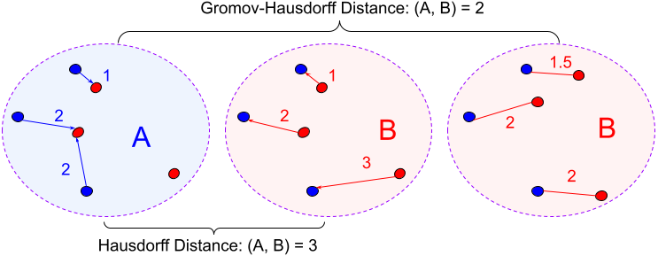
Figure 2: Calculation of Gromov-Hausdorff (GH) Distance: the worst case distance of nearest neighbors in a shared embedding space after optimal orthogonal mapping. The right-most red dots have been orthogonally rotated to turn Hausdorff distance into GH Distance.

4 Method

We implement Skip-gram with negative sampling on GPU using PyTorch and use it to train monolingual embedding spaces for Bengali (bn), Ukranian (uk), Tamil (ta), and English (en). Our implementation mirrors the official word2vec release closely Mikolov et al. (2013a).

We create comparison embedding spaces using the official word2vec release with default hyperparameters and map the resulting spaces from both algorithms with VecMap for BLI. We report precision@1 (P@1) on the development set in Table 1. P@1 is a standard evaluation metric for BLI. Our implementation slightly outperforms word2vec except ta in unsupervised mode.

		bn-en			uk-en			ta-en
		Su	Se	U	Su	Se	U	Su	Se	U
W2V	$\mu$	12.6	11.9	9.0	10.8	9.7	7.7	8.4	7.3	7.1
	$\sigma$	0.3	0.3	5.0	0.5	0.4	4.3	0.5	0.6	0.6
Ours	$\mu$	13.1	12.2	10.8	12.4	11.7	10.5	9.3	8.3	1.8
	$\sigma$	1.0	0.4	0.9	0.9	0.5	0.6	0.7	0.9	3.7

Table 1: P@1 of mapped embedding spaces on the development set: our implementation vs. official word2vec release. Shown: Mean ($\mu$) and standard deviation ($\sigma$) over 5 runs in supervised (Su), semi-supervised (Su), and unsupervised (U) modes.

newscrawl2020				Common Crawl	newscrawl2018-20
en	bn	ta	uk	en	en
29.0	14.7	12.6	7.8	750	2700

Table 2: Size of training data (millions of tokens).

4.1 Data

For the main experiments, we train word embeddings on the first 1 million lines from newscrawl2020 for en, bn, and ta Barrault et al. (2020). For uk, we use the entirety of newscrawl2020 ($\sim$427,000 lines). We normalize punctuation, lowercase, remove non-printing characters, and tokenize using standard Moses scripts. Domain mismatch experiments in Section 5.2 use approximately 33.8 million lines of webcrawl from the English Common Crawl. Larger data experiments in the same section use 93 million lines of English newscrawl2018-2020. The size of the training data in tokens is seen in Table 2.

We use the publicly available train and test dictionaries from MUSE Lample et al. (2018). For the development set, we use source words 6501-8000 from the “full” set. Train, development, and test sets are non-overlapping. We use all possible training set seed words for our supervised losses, which is 6000-7000 word pairs per language. We use the test set for evaluating downstream BLI.

4.2 Integrating Isomorphism Losses

To train the embedding space $\bf{X}$ such that it 1) captures the distributional information via Skip-gram with negative sampling and 2) is geometrically similar to the reference word embedding space $\bf{Y}$, we propose the objective below. $\mathcal{L}_{SG}$ is the familiar Skip-gram with negative sampling loss function and $\mathcal{L}_{ISO}$ is the isomorphism metric loss. Each $\mathcal{L}_{ISO}$ requires a reference embedding space $\bf{Y}$, trained separately using our base implementation.

$$\mathcal{L}=(1-\beta)\,\mathcal{L}_{SG}+\beta\,\mathcal{L}_{ISO}$$

We use English as the reference language because we generally assume that the data quality is higher than the low-resource languages used on the source-side. $\bf{Y}$ is normalized, mean-centered, and normalized again before use. On each calculation of $\mathcal{L}_{ISO}$, we perform the same operations on a copy of the current model’s word embeddings.

4.3 Supervised Losses

We assume seeds $\{(x_{0},y_{0}),(x_{1},y_{1}),...(x_{s},y_{s})\}$. $X$ is a matrix of the current model’s word embeddings for [$x_{0},x_{1},...,x_{s}$] and $Y$ is the matrix of reference source embeddings for [$y_{0},y_{1},...,y_{s}$].

L2

We implement L2 distance and normalize over samples. Intuitively, this coaxes translation pairs to have similar vector representations, with the hope that other words in $\bf{X}$ and $\bf{Y}$ will be tugged closer to their translations. L2 is easy to implement and understand, and computes quickly.

$$\frac{1}{|X|}\sum_{i=1}^{s}||x_{i}-y_{i}||_{2}$$

Proc-L2

We find $W$ that solves the orthogonal Procrustes problem as in Section 3.1, then minimize L2 distance over the mapped space:

$$\frac{1}{|X|}\sum_{i=1}^{s}||x_{i}W-y_{i}||_{2}$$

Proc-L2+Init

Same as Proc-L2, except initialize source seed embeddings with the reference translation vectors so that spaces begin with the same representation for known translations.

RSIM

We implement relational similarity over seeds. Higher is better, so we minimize $\mathcal{L}_{ISO}=1-\text{Pearsons\_Corr}$. Like Proc-L2+Init, we can also initialize the source space with reference seed embeddings. We call this RSIM+Init.

4.4 Unsupervised Losses

We use two unsupervised metrics to increase isomorphism when no seed translations are available.

RSIM-U

In this unsupervised variant of RSIM, we calculate pairwise cosine similarities over the first $k$ words in $\bf X$ and $\bf Y$, sort the lists, then calculate Pearson’s correlation. As above, $\mathcal{L}_{ISO}=1-\text{Pearsons\_Corr}$. We use $k=2000$ for efficiency.

EVS-U

We calculate eigenvector similarity over the first 2000 words in $\bf X$ and $\bf Y$.

4.5 On Differentiability

Each metric must be differentiable with respect to $\bf X$, a matrix of the model’s current word embeddings, to allow isomorphism-based losses to inform parameter updates in $\bf X$.

L2 is straightforwardly differentiable, as it is the Frobenius norm of $X-Y$. The same applies for variants Proc-L2 and Proc-L2+Init. RSIM is naturally differentiable, seen in the formulation below. For mean-centered cosine similarity vectors $x_{sim}$ and $y_{sim}$, Pearson’s correlation coefficient is:

$$\frac{\sum_{i}x_{sim}(i)y_{sim}(i)}{\sqrt{\sum_{i}x_{sim}(i)^{2}y_{sim}(i)^{2}}}=\frac{x_{sim}^{T}y_{sim}}{\lVert x_{sim}\rVert\lVert y_{sim}\rVert}$$

EVS is not immediately differentiable due to the need for the non-differentiable $k$-NN computation. Instead we modify the graph computation step to use a fully-connected weighted graph where the edge weight is the dot product between node vectors. With this amended formulation, computing the gradients of Laplacian eigenvalues is possible.

4.6 $\beta$ and Linear Mapping for BLI

Each isomorphism loss may be considered a different method, as each loss may cause the overall framework to behave differently. Accordingly, we set $\beta$ for each separate loss function based on performance on the development set. After selecting $\beta$, we evaluate and present results only on the test set. $\beta$s for each method are in Table 3.

	L2	Proc-L2	+Init	RSIM	+Init	-U	EVS-U
$\beta$	0.1	0.333	0.2	0.01	0.001	0.1	0.333

Table 3: $\beta$ parameter for isomorphism losses. Each loss function should be considered a separate method, so $\beta$ is set for each loss based on development set performance. Once $\beta$ is chosen, we evaluate on the test set.

VecMap in supervised mode consistently scores higher than semi-supervised mode in all baseline experiments on the development set. For IsoVec, semi-supervised mapping often works best. We thus use VecMap in supervised mode for baselines and semi-supervised mode for IsoVec supervised runs. This sometimes underestimates IsoVec’s strength when supervised mapping would have performed better. For unsupervised experiments and baselines, we map in unsupervised mode. Each is run five times and averaged. IsoVec and VecMap use one NVIDIA GeForce GTX 1080Ti GPU.

5 Experiments & Results

We pretrain English embeddings to use as reference space $\bf{Y}$. IsoVec trains source space $\bf{X}$.

5.1 Main Experiments

For baselines, we train source and target spaces separately for each run using our base implementation. In experimental conditions, we train the source space with IsoVec using each isomorphism loss from Sections 4.3 and 4.4. In Table 4, we see that IsoVec consistently outperforms the baseline for bn-en and uk-en. For ta-en, it outperforms with Proc-L2+Init and both unsupervised methods. In terms of training efficiency, L2-based methods perform comparably to the baseline (< 10% time increase) and RSIM-based methods see a slight time increase ($\sim$10-16% increase over baseline). EVS-based methods require an expensive eigendecomposition step which causes a $\sim$2.5x time increase over the baseline.

	bn		uk		ta
Supervised	$\mu$	$\sigma$	$\mu$	$\sigma$	$\mu$	$\sigma$
Baseline	15.2	(0.8)	14.4	(0.8)	11.6	(0.4)
L2	16.3	(0.4)	16.5	(0.4)	11.1	(0.5)
Proc-L2	16.6	(0.7)	16.0	(0.8)	10.7	(0.3)
+Init	16.9	(0.2)	17.1	(0.6)	11.8	(0.3)
RSIM	16.3	(0.3)	15.9	(0.4)	10.3	(0.6)
+Init	16.0	(0.4)	17.1	(0.5)	11.0	(0.4)
Unsupervised
Baseline	13.2	(0.6)	12.6	(0.5)	3.2	(4.4)
RSIM-U	14.2	(0.7)	14.0	(0.6)	5.4	(4.9)
EVS-U	13.4	(0.7)	13.4	(0.6)	5.2	(4.8)

Table 4: Main Experiments. Average P@1 ($\mu$) and standard deviation ($\sigma$) over 5 runs of IsoVec with isomorphism losses for bn-en, uk-en, ta-en.

5.2 Algorithm, Domain, & Data Mismatch

Søgaard et al. (2018) show that mapping methods fail for embeddings trained with different algorithms, and that BLI performance deteriorates when source and target domains do not match (Marchisio et al., 2020). We test IsoVec under algorithm and domain mismatch using the best losses from the main experiments: Proc-L2+Init and RSIM-U. We use $\beta$ as-is from the previous section.

The IsoVec base model intends to mirror word2vec closely, but there are likely output differences due to implementation. We map the baseline source embeddings trained in the main experiments to varying en target spaces trained with the official word2vec release, so that algorithms do not match between source and target embedding spaces. We run experiments using the below training data:

• Algorithm Mismatch: 1 million lines of en newscrawl2020 (same as main experiments). Shows effect of algorithm mismatch only.

• +More Target-Side Data: 93 million lines of en newscrawl2018-20. Shows effect of target trained with ample in-domain data.

• +Domain Mismatch: 33.8 million lines of en Common Crawl (web-crawl). Shows the effect of different domains in source vs. target.

Table 5 contains baselines for our mismatch experiments and shows the drop in performance compared to Table 4 baselines, where both source and target embedding spaces were trained with the IsoVec base model. This occurs across languages, moderately for supervised baselines, and severely for unsupervised. The large performance drop given more high-quality data of the same domain in unsupervised mode (+More Target-Side Data) is surprising given that this target space is stronger than the one from only Algorithm Mismatch. Perhaps its geometry has changed so considerably because of its additional data and different algorithm that it is too different from the lower-resource source space to be mapped with unsupervised methods. This should be investigated in future work.

	Supervised									Unsupervised
	bn			uk			ta			bn			uk			ta
	$\mu$	$\Delta$	$\sigma$	$\mu$	$\Delta$	$\sigma$	$\mu$	$\Delta$	$\sigma$	$\mu$	$\Delta$	$\sigma$	$\mu$	$\Delta$	$\sigma$	$\mu$	$\Delta$	$\sigma$
Main Baseline	15.2	-	0.8	14.4	-	0.8	11.6	-	0.4	13.2	-	0.6	12.6	-	0.5	3.2	-	4.4
Algorithm Mism.	13.6	(-1.6)	0.5	11.7	(-2.7)	0.6	9.4	(-2.1)	0.5	11.9	(-1.3)	0.7	4.4	(-8.2)	6.1	2.6	(-0.6)	3.6
+More Trg Data	16.0	(+0.8)	0.7	13.5	(-0.9)	0.3	11.0	(-0.6)	0.6	5.9	(-7.3)	8.0	0.0	(-12.6)	0.0	0.0	(-3.2)	0.0
+Domain Mism.	10.5	(-4.7)	0.6	10.0	(-4.4)	0.4	8.4	(-3.2)	0.4	0.0	(-13.2)	0.0	0.0	(-12.6)	0.0	0.0	(-3.2)	0.0

Table 5: Effect of algorithm and data mismatch in source vs. target embedding spaces. Average P@1 of 5 runs ($\mu$) with $\Delta$ vs. baseline and std.dev. ($\sigma$). Isomorphism losses are not used here. Source-side embeddings are trained with our base implementation, target-side with word2vec (algorithm mismatch). Main Baseline is from the main experiments, Table 4. +More Target-Side Data (+More Trg Data) uses nearly 100x more data on the target-side than previous experiments. +Domain Mismatch uses target embeddings trained on $\sim 34$M lines of web crawl.

We run Proc-L2+Init and RSIM-U in Algorithm Mismatch, +More Target-Side Data, and +Domain Mismatch conditions as described above. Results are in Table 6. In supervised mode, IsoVec recovers from algorithm mismatch by 2.7-4.9 points, domain mismatch by 2.5-7.3, and still improves when the target space is trained on $\sim$100x more data. Whereas +Domain Mismatch and +More Target-Side Data baselines fail to extract any correct translation pairs in unsupervised mode, RSIM-U method completely recovers in all conditions: equalling or outperforming the main unsupervised baseline from Table 4 which matched on algorithm, domain, and data size. IsoVec is thus useful for many types of distributional shifts: algorithmic, domain, and amount of data available.

	Algorithm Mismatch						+ Domain Mismatch						+ More Target-Side Data
	bn		uk		ta		bn		uk		ta		bn		uk		ta
	$\mu$	$\sigma$	$\mu$	$\sigma$	$\mu$	$\sigma$	$\mu$	$\sigma$	$\mu$	$\sigma$	$\mu$	$\sigma$	$\mu$	$\sigma$	$\mu$	$\sigma$	$\mu$	$\sigma$
Supervised
Baseline	13.6	(0.5)	11.7	(0.6)	9.4	(0.5)	10.5	(0.6)	10.0	(0.4)	8.4	(0.4)	16.0	(0.7)	13.5	(0.3)	11.0	(0.6)
Proc-L2+I (Ours)	16.3	(0.4)	16.6	(2.2)	12.1	(0.7)	15.5	(0.7)	17.3	(0.4)	10.9	(0.5)	16.2	(0.4)	17.3	(0.3)	11.4	(0.3)
Unsupervised
Baseline	11.9	(0.7)	4.4	(6.1)	2.6	(3.6)	0.0	(0.0)	0.0	(0.0)	0.0	(0.0)	5.9	(8.0)	0.0	(0.0)	0.0	(0.0)
RSIM-U (Ours)	13.6	(0.7)	13.4	(1.2)	3.6	(4.8)	13.5	(0.7)	13.1	(0.8)	6.8	(3.8)	14.4	(0.7)	13.6	(0.6)	3.2	(4.3)

Table 6: P@1 of IsoVec vs. baseline under algorithm and domain mismatch. Baselines correspond to Table 5 results. Ours, Supervised: Proc-L2+Init. Ours, Unsupervised: RSIM-U.

5.3 Effect on Isomorphism

Table 7 (left) shows the effect of IsoVec on global isomorphism measures. We measure relational similarity, eigenvector similarity, and Gromov-Hausdorff distance of trained embedding spaces (before mapping) for all main experiments of Section 5.1 using scripts from Vulić et al. (2020). We average over experiments. To avoid confusion with the IsoVec loss functions, we call the metrics “RelSim”, “EigSim”, and “GH”. The script calculates EigSim ($k=2$) over the first 10,000 embeddings in each space and GH over the first 5000. RelSim is calculated over the first 1000 seed translation pairs.

All supervised methods improved RelSim ($\uparrow$ better). Perhaps surprisingly, initializing the source space with target embeddings (+Init) worsens isomorphism. RSIM is best, directly optimizing for this metric in a supervised manner. RelSim stayed roughly consistent in unsupervised experiments.

All uk-en and ta-en experiments improve GH (Patra et al., 2019, $\downarrow$ better). GH worsened for bn-en despite improved BLI (Table 4). EigSim ( $\downarrow$ better) improves across all experiments except uk-en supervised methods, despite improved BLI (notably, initial EigSim for uk was low). EVS-U strongly improves EigSim, optimizing it directly. Table 7 (left) measures the unperturbed geometry of spaces after training and shows that IsoVec improves isomorphism in a majority of settings. The same calculation over embeddings after mapping with semi-supervised VecMap is in Table A.1.

It is interesting that baseline experiments performed better when mapped in supervised mode while spaces trained with IsoVec tended to map better in semi-supervised mode (as mentioned in Section 4.6). This may further indicate that the IsoVec spaces have become more geometrically similar.

	Relational Sim. $\uparrow$			GH Distance $\downarrow$			Eigenvector Sim. $\downarrow$
	bn	uk	ta	bn	uk	ta	bn	uk	ta
Baseline	0.32	0.26	0.27	0.34	1.17	0.39	62.7	49.9	74.7
L2	0.36	0.34	0.33	0.43	0.76	0.19	52.0	68.5	47.3
Proc-L2	0.43	0.42	0.39	0.42	0.51	0.23	46.6	72.8	37.7
+Init	0.39	0.38	0.35	0.43	0.46	0.22	52.1	77.2	41.0
RSIM	0.54	0.53	0.47	0.37	0.56	0.20	47.2	60.4	39.8
+Init	0.37	0.35	0.33	0.40	0.52	0.20	48.6	65.6	44.8
RSIM-U	0.30	0.25	0.26	0.42	0.54	0.32	56.3	36.2	60.1
EVS-U	0.30	0.24	0.26	0.68	0.53	0.30	38.7	38.3	39.5

		All	bn-en	uk-en	ta-en
P@1   vs. RelSim	(+)	0.17	-0.03	-0.54	-0.54
vs. GH	(-)	0.79	0.28	-0.23	0.27
vs. EigSim	(-)	0.57	0.17	-0.05	0.05
RelSim    vs. GH	(-)	0.09	-0.45	-0.24	-0.03
vs. EigSim	(-)	-0.05	-0.25	-0.28	-0.27
GH     vs. EigSim	(+)	0.65	-0.16	-0.17	-0.29

Table 7: Left: Isomorphism scores of source vs. target embedding space after training, per language, per training method, averaged over 5 runs. Best is bold. IsoVec output embeddings vs. base English space. Right: Pearson’s correlation: BLI performance (P@1) of supervised IsoVec experiments vs. isomorphism score and between metrics. (+/-): expected direction of correlation: opposite or weak (magnitude <= 0.05).

6 Discussion

6.1 The Promise of Geometric Losses

We have seen that IsoVec improves relative isomorphism and downstream BLI from word embedding spaces. The success of unsupervised methods is particularly encouraging for the use of global isomorphism measures to improve embedding spaces. Notably, we use only the first 2000 words per space to calculate unsupervised IsoVec losses—i.e., we coax these frequent words to have similar representations, regardless of identity. While there are likely some true translation pairs in the mix, there are almost certainly words this subset of $\bf{X}$ whose translation is not in the first 2000 words of $\bf{Y}$ (and vice-versa)—particularly when source and target corpora are from different domains. Regardless, IsoVec unsupervised methods work.

6.2 Need for a Sensitive Isomorphism Metric

Previous authors found that EigSim and GH correlate well with BLI performance Søgaard et al. (2018); Patra et al. (2019), however our results reveal a nuanced story. In Table 7 (right), we correlate the EigSim, RelSim, and GH with BLI P@1 performance over all runs of the main supervised IsoVec experiments (L2, Proc-L2, Proc-L2+Init, RSIM, RSIM+Init; 25 data points per calculation).

P@1 should correlate positively with RelSim ($\uparrow$ better for both) and negatively vs. GH/EigSim ($\downarrow$ better for GH/EigSim). RelSim should correlate negatively with GH/EigSim, and GH positively with EigSim. In Table 7 (right) within language, however, only P@1 vs. GH on uk-en aligns with intuition. Many correlations are weak (gray, magnitude <= 0.05) or opposite of expected; For instance, P@1 should increase with RelSim, but we see the opposite within language pair. Over languages combined, the relationship is weakly positive. Figure A.1 shows how this is possible.

Samples for Pearson’s correlation should be drawn from the same population, and in Table 7 (right) we assume that is our IsoVec embedding spaces. Perhaps the assumption is unfair: different IsoVec losses might induce different monolingual spaces where specific metrics are indeed predictive of downstream BLI performance, but this may not be visible in the aggregate. An ideal metric, however, would predict downstream BLI performance regardless of how monolingual spaces were trained; such that we might assess the potential of spaces to align well without having to map them and measure their performance with development or test dictionaries. In that light, the discrepancies in Table 7 (right) highlight the need for a more sensitive metric that works within language and with small differences in BLI performance.

We should thus be cautious drawing between- vs. within-language conclusions about isomorphism metrics and downstream BLI. When isomorphism metrics differ considerably, perhaps BLI performance also differs similarly, as seen in previous work; however if isomorphism scores are poor or too similar, the metrics may not be sensitive enough to be predictive. Future work should investigate these hypotheses and develop isomorphism metrics that are more sensitive. The spectral measures of Dubossarsky et al. (2020) might be examined in these lower-resource contexts, as the authors claim to correlate better with downstream BLI. All-in-all, though, our main results show that coaxing towards improved isomorphism as measured by the three popular metrics can improve BLI performance even if the scores are not strongly predictive of raw P@1.

7 Conclusion & Future Work

We present IsoVec, a new method for training word embeddings which directly injects global measures of embedding space isomorphism into the Skip-gram loss function. Our three supervised and two unsupervised isomorphism loss functions successfully improve the mappability of monolingual word embedding spaces, leading to improved ability to induce bilingual lexicons. IsoVec also shows promise under algorithm mismatch, domain mismatch, and data size mismatch between source and target training corpora. Future work could extend our work to even greater algorithmic mismatches, and in massively multilingual contextualized models. We release IsoVec at https://github.com/kellymarchisio/isovec.

Limitations

As with most methods based on static word embeddings, our work is limited by polysemy. By using word2vec as a basis, we inherit many of its limitations, many of which are addressed in recent contextualized representation learning work. Future work might apply our methods to contextualized models. We also experiment with only English as a target language, limiting our method’s universal applicability. Future work could extend our results to non-English pairs, and also evaluate monolingually if languages will be used separately as recommended by Luong et al. (2015).

Appendix A Appendix

We wrote the proofs in Sections A.1 and A.2 in the process of understanding the advanced mapping procedure of VecMap. The interested reader may find them elucidating.

A.1 Whitening Transformations

Estimating the covariance matrix.

Let $X\in\mathbb{R}^{n\times d}$ be a data matrix of $n$ samples of $d$ dimensions. We mean-center $X$ dimension-wise, then recall that the below is an unbiased estimator over $n$ samples of the covariance matrix of $X$.

$$\Sigma_{X}=\frac{1}{(n-1)}{X}^{T}{X}$$

The whitening matrix.

The goal of a whitening transformation is to transform $X$ into a data matrix $Z\in\mathbb{R}^{n\times d}$ such that all dimensions are uncorrelated and have unit variance, meaning that the covariance matrix $\Sigma_{Z}=\frac{1}{(n-1)}{Z}^{T}{Z}=I$. Doing so ensures that each basis vector in the space of $Z$ is minimally correlated with all others, and therefore retains maximal explanatory power. We may state the whitening objective as finding $W$ such that $Z=XW^{T}$ and $\Sigma_{Z}=I$. Let $c=\frac{1}{n-1}$, so that $\Sigma_{Z}=c{Z}^{T}{Z}$.

We claim that for $W$, if $W^{T}W=\Sigma_{X}^{-1}$, we obtain a valid whitening matrix:

$$cZ^{T}ZW =c(XW^{T})^{T}XW^{T}W$$

$$=cWX^{T}XW^{T}W$$

$$=W\Sigma_{X}W^{T}W$$

$$=W\Sigma_{X}\Sigma_{X}^{-1}$$

$$=W$$

Therefore, since $cZ^{T}ZW=W$, $cZ^{T}Z=I$. There are infinite solutions for $W^{T}W=\Sigma_{X}^{-1}$. A common choice called “ZCA Whitening” selects $W_{ZCA}=\Sigma_{X}^{-\frac{1}{2}}$. See Kessy et al. (2018) for a similar derivation and head-to-head comparison of 5 whitening methods.

VecMap’s whitening is proportional to ZCA.

VecMap’s whitening chooses $W_{vecmap}=VS^{-1}V^{T}$, where $USV^{T}=\text{SVD}(X)$. We show that this choice is proportional to ZCA Whitening, and furthermore that it is a valid whitening matrix.

First, we show that $W_{vecmap}$ is proportional to $W_{ZCA}=\Sigma_{X}^{-\frac{1}{2}}$. Note that $S^{T}=S$ and that $S^{-1}$ can be written as $\frac{1}{S}$ because $S$ is diagonal.

$$\Sigma_{X} =c(USV^{T})^{T}USV^{T}$$

$$=cVS^{T}U^{T}USV^{T}$$

$$=cVS^{2}V^{T}$$

$$\implies\Sigma_{X}^{\frac{1}{2}} =\sqrt{c}VSV^{T}$$

$$\implies W_{ZCA}=\Sigma_{X}^{-\frac{1}{2}} =\frac{1}{\sqrt{c}}VS^{-1}V^{T}$$

$$\propto W_{vecmap}$$

$\bf{W_{vecmap}}$ is a valid whitening matrix.

Let $Z=XW_{vecmap}^{T}$. We claim that if $Z=XW_{vecmap}^{T}$, then $\Sigma_{Z}=cZ^{T}Z=I$. We assume $X$ is unit-normalized and mean-centered.

$$cZ^{T}Z =c(XW^{T})^{T}XW^{T}=cWX^{T}XW^{T}$$

$$=cVS^{-1}V^{T}X^{T}X(VS^{-1}V^{T})^{T}$$

$$=cVS^{-1}V^{T}X^{T}XVS^{-1}V^{T}$$

$$=cVS^{-1}V^{T}(USV^{T})^{T}USV^{T}VS^{-1}V^{T}$$

$$=cVS^{-1}V^{T}VSU^{T}USV^{T}VS^{-1}V^{T}$$

$$=cI$$

A.2 Derivation of Orthogonal Mapping Variant Before Dictionary Induction in VecMap

The orthogonal mapping performed at the final step of VecMap is a variant of the orthogonal Procrustes problem. VecMap finds the matrices $W_{x}$ and $W_{z}$ such that $XW_{x}$ and $ZW_{z}$ are maximally close to each other. This is equivalent to minimizing $||ZWz-XWx||$. The solution is $W_{z}=U$ and $Wx=V$ where $USV^{T}=\text{SVD}(X^{T}Z)$. Observe the derivation below, where we use the Frobenius norm/inner product:

$$\underset{W_{x},W_{x}}{\arg\min}||ZW_{z}-XW_{x}||$$

$$= \underset{W_{x},W_{x}}{\arg\min}\langle ZW_{z}-XW_{x},ZW_{z}-XW_{x}\rangle$$

$$= \underset{W_{x},W_{x}}{\arg\min}\langle ZW_{z},ZW_{z}\rangle-2\langle XW_{x},ZW_{z}\rangle$$

$$\;\;\;\;\;\;\;\;\;\;\;\;\;\;\;\;\;\;\;\;\;\;\;\;\;\;\;\;+\langle XW_{x},XW_{x}\rangle$$

$$= \underset{W_{x},W_{x}}{\arg\min}||Z||^{2}-2\langle XW_{x},ZW_{z}\rangle+||X||^{2}$$

$$= \underset{W_{x},W_{x}}{\arg\min}-2\langle XW_{x},ZW_{z}\rangle$$

$$= \underset{W_{x},W_{x}}{\arg\max}\langle XW_{x},ZW_{z}\rangle$$

$$= \underset{W_{x},W_{x}}{\arg\max}\text{ Trace}(W_{z}^{T}Z^{T}XW_{x})$$

Given the cyclic property of the trace, the objective is equivalent to maximizing $\text{ Trace}(XW_{x}W_{z}^{T}Z^{T})$, as stated by Artetxe et al. (2018a).

A.3 RSIM vs. P@1: Pearson’s Correlation

Figure A.1 shows relational similarity score vs. P@1 over all language pairs described in Section 5.3. We observe how it is possible to have within-language negative correlations but a positive overall correlation.

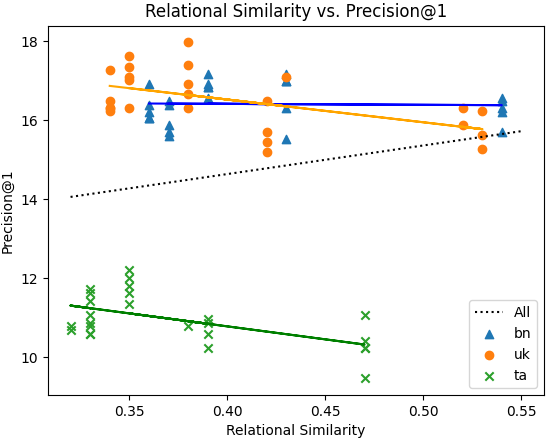
Figure A.1: Relational similarity vs. P@1 for all supervised IsoVec experiments (See Section 5.3).

A.4 Effect on Isomorphism, After Mapping

	Relational Sim. $\uparrow$			GH Distance $\downarrow$			Eigenvector Sim $\downarrow$
	bn	uk	ta	bn	uk	ta	bn	uk	ta
Baseline	0.43	0.35	0.38	0.41	1.02	0.42	92.8	113.8	133.3
L2	0.47	0.41	0.41	0.36	0.91	0.38	97.8	145.3	98.3
Proc-L2	0.51	0.48	0.45	0.35	0.81	0.37	87.4	148.2	96.8
+Init	0.48	0.44	0.43	0.37	0.68	0.35	97.4	155.4	99.4
RSIM	0.65	0.62	0.59	0.34	0.71	0.40	43.2	108.8	69.2
+Init	0.48	0.45	0.43	0.37	0.62	0.37	95.5	126.4	96.6
RSIM-U	0.43	0.35	0.37	0.37	0.59	0.44	94.6	121.9	135.5
EVS-U	0.43	0.35	0.37	0.48	0.64	0.49	83.1	109.4	110.7

Table A.1: Isomorphism scores of source vs. reference embedding space after training and mapping with VecMap. All experiments are mapped in semi-supervised mode. Results averaged over 5 runs. Best score is bold.

Comparing with Table 7 in the main body of this paper, Table A.1 shows average isomorphism scores of source vs. reference embedding spaces after mapping with VecMap in semi-supervised mode. RSIM best improves relational similarity and eigenvector similarity. GH distance improves for supervised methods and RSIM-U.

Table 7 measures the unperturbed geometry of the space after applying IsoVec. Importantly, RelSim, GH, and EigSim do not require mapping for measurement, as they are invariant to transformation (RelSim and EigSim measure nearest-neighbor graphs, and GH measures nearest neighbor after optimal isometric transform). Table A.1, measures a geometry that may have been perturbed due to VecMap operations such as whitening/dewhitening. While isomorphism scores over the mapped spaces appear more consistent in terms of internal patterns, Table 7 measures isomorphism induced directly by IsoVec, whereas Table A.1 may be influenced by VecMap as well.

		Overall	bn-en	uk-en	ta-en
P@1   vs. RelSim	(+)	0.13	-0.16	-0.49	-0.59
vs. GH	(-)	0.39	0.02	-0.42	-0.79
vs. EigSim	(-)	0.31	0.22	0.15	-0.29
RelSim   vs. GH	(-)	-0.12	-0.54	-0.20	0.51
vs. EigSim	(-)	-0.54	-0.88	-0.57	-0.10
GH    vs. EigSim	(+)	0.72	0.57	0.23	0.72

Table A.2: Pearson’s Correlations: BLI performance (P@1) vs. relational similarity, Gromov-Hausdorff Distance, and eigenvector similarity score of trained source embeddings vs. English reference space, after VecMap mapping in semi-supervised mode, and isomorphism metrics correlated amongst themselves. Computed over supervised IsoVec experiments (ex. P@1 vs. RelSim for bn-en is P@1 from all runs of L2, Proc-L2, Proc-L2+I, RSIM, RSIM-Init with RelSim/GH/EigSim for each.) Directly comparable to Table 7 (right).

		Overall	bn-en	uk-en	ta-en
P@1   vs. RelSim	(+)	0.29	0.44	0.39	0.14
vs. GH	(-)	0.34	-0.26	0.19	-0.78
vs. EigSim	(-)	0.14	0.00	0.42	-0.29
RelSim   vs. GH	(-)	-0.15	-0.33	0.21	-0.34
vs. EigSim	(-)	-0.48	-0.75	-0.06	-0.69
GH    vs. EigSim	(+)	0.63	0.20	0.33	0.31

Table A.3: Same as Table A.2, except computed over all IsoVec experiments (L2, Proc-L2, Proc-L2+I, RSIM, RSIM-Init, RSIM-U, EVS-U).

Table A.2 shows correlations after mapping over only the supervised IsoVec methods. Compared with Table 7 (right), we see that relationships between the isomorphism measures are more aligned with our expectations now, but still no isomorphism measure is consistently predictive of P@1 across languages. Table A.3 shows the same calculations over all IsoVec experiments mapped in semi-supervised mode, though unsupervised training with semi-supervised mapping probably would not be used in practice as it is here for RSIM-U and EVS-U.

References

- Alvarez-Melis and Jaakkola (2018) David Alvarez-Melis and Tommi Jaakkola. 2018. Gromov-Wasserstein alignment of word embedding spaces. In Proceedings of the 2018 Conference on Empirical Methods in Natural Language Processing, pages 1881–1890, Brussels, Belgium. Association for Computational Linguistics.
- Artetxe et al. (2016) Mikel Artetxe, Gorka Labaka, and Eneko Agirre. 2016. Learning principled bilingual mappings of word embeddings while preserving monolingual invariance. In Proceedings of the 2016 Conference on Empirical Methods in Natural Language Processing, pages 2289–2294, Austin, Texas. Association for Computational Linguistics.
- Artetxe et al. (2017) Mikel Artetxe, Gorka Labaka, and Eneko Agirre. 2017. Learning bilingual word embeddings with (almost) no bilingual data. In Proceedings of the 55th Annual Meeting of the Association for Computational Linguistics (Volume 1: Long Papers), pages 451–462, Vancouver, Canada. Association for Computational Linguistics.
- Artetxe et al. (2018a) Mikel Artetxe, Gorka Labaka, and Eneko Agirre. 2018a. Generalizing and improving bilingual word embedding mappings with a multi-step framework of linear transformations. In Proceedings of the AAAI Conference on Artificial Intelligence, volume 32.
- Artetxe et al. (2018b) Mikel Artetxe, Gorka Labaka, and Eneko Agirre. 2018b. A robust self-learning method for fully unsupervised cross-lingual mappings of word embeddings. In Proceedings of the 56th Annual Meeting of the Association for Computational Linguistics (Volume 1: Long Papers), pages 789–798, Melbourne, Australia. Association for Computational Linguistics.
- Barrault et al. (2020) Loïc Barrault, Magdalena Biesialska, Ondřej Bojar, Marta R. Costa-jussà, Christian Federmann, Yvette Graham, Roman Grundkiewicz, Barry Haddow, Matthias Huck, Eric Joanis, Tom Kocmi, Philipp Koehn, Chi-kiu Lo, Nikola Ljubešić, Christof Monz, Makoto Morishita, Masaaki Nagata, Toshiaki Nakazawa, Santanu Pal, Matt Post, and Marcos Zampieri. 2020. Findings of the 2020 conference on machine translation (WMT20). In Proceedings of the Fifth Conference on Machine Translation, pages 1–55, Online. Association for Computational Linguistics.
- Cao et al. (2020) Steven Cao, Nikita Kitaev, and Dan Klein. 2020. Multilingual alignment of contextual word representations. In International Conference on Learning Representations.
- Chazal et al. (2009) Frédéric Chazal, David Cohen-Steiner, Leonidas J. Guibas, Facundo Mémoli, and Steve Y. Oudot. 2009. Gromov-hausdorff stable signatures for shapes using persistence. Computer Graphics Forum, 28(5):1393–1403.
- Conneau et al. (2020) Alexis Conneau, Kartikay Khandelwal, Naman Goyal, Vishrav Chaudhary, Guillaume Wenzek, Francisco Guzmán, Edouard Grave, Myle Ott, Luke Zettlemoyer, and Veselin Stoyanov. 2020. Unsupervised cross-lingual representation learning at scale. In Proceedings of the 58th Annual Meeting of the Association for Computational Linguistics, pages 8440–8451, Online. Association for Computational Linguistics.
- Czarnowska et al. (2019) Paula Czarnowska, Sebastian Ruder, Edouard Grave, Ryan Cotterell, and Ann Copestake. 2019. Don’t forget the long tail! a comprehensive analysis of morphological generalization in bilingual lexicon induction. In Proceedings of the 2019 Conference on Empirical Methods in Natural Language Processing and the 9th International Joint Conference on Natural Language Processing (EMNLP-IJCNLP), pages 974–983, Hong Kong, China. Association for Computational Linguistics.
- Devlin et al. (2019) Jacob Devlin, Ming-Wei Chang, Kenton Lee, and Kristina Toutanova. 2019. BERT: Pre-training of deep bidirectional transformers for language understanding. In Proceedings of the 2019 Conference of the North American Chapter of the Association for Computational Linguistics: Human Language Technologies, Volume 1 (Long and Short Papers), pages 4171–4186, Minneapolis, Minnesota. Association for Computational Linguistics.
- Doval et al. (2018) Yerai Doval, Jose Camacho-Collados, Luis Espinosa-Anke, and Steven Schockaert. 2018. Improving cross-lingual word embeddings by meeting in the middle. In Proceedings of the 2018 Conference on Empirical Methods in Natural Language Processing, pages 294–304, Brussels, Belgium. Association for Computational Linguistics.
- Dubossarsky et al. (2020) Haim Dubossarsky, Ivan Vulić, Roi Reichart, and Anna Korhonen. 2020. The secret is in the spectra: Predicting cross-lingual task performance with spectral similarity measures. In Proceedings of the 2020 Conference on Empirical Methods in Natural Language Processing (EMNLP), pages 2377–2390, Online. Association for Computational Linguistics.
- Eder et al. (2021) Tobias Eder, Viktor Hangya, and Alexander Fraser. 2021. Anchor-based bilingual word embeddings for low-resource languages. In Proceedings of the 59th Annual Meeting of the Association for Computational Linguistics and the 11th International Joint Conference on Natural Language Processing (Volume 2: Short Papers), pages 227–232, Online. Association for Computational Linguistics.
- Ethayarajh (2019) Kawin Ethayarajh. 2019. How contextual are contextualized word representations? Comparing the geometry of BERT, ELMo, and GPT-2 embeddings. In Proceedings of the 2019 Conference on Empirical Methods in Natural Language Processing and the 9th International Joint Conference on Natural Language Processing (EMNLP-IJCNLP), pages 55–65, Hong Kong, China. Association for Computational Linguistics.
- Ethayarajh and Jurafsky (2021) Kawin Ethayarajh and Dan Jurafsky. 2021. Attention flows are shapley value explanations. In Proceedings of the 59th Annual Meeting of the Association for Computational Linguistics and the 11th International Joint Conference on Natural Language Processing (Volume 2: Short Papers), pages 49–54, Online. Association for Computational Linguistics.
- Faruqui et al. (2015) Manaal Faruqui, Jesse Dodge, Sujay Kumar Jauhar, Chris Dyer, Eduard Hovy, and Noah A. Smith. 2015. Retrofitting word vectors to semantic lexicons. In Proceedings of the 2015 Conference of the North American Chapter of the Association for Computational Linguistics: Human Language Technologies, pages 1606–1615, Denver, Colorado. Association for Computational Linguistics.
- Glavaš et al. (2019) Goran Glavaš, Robert Litschko, Sebastian Ruder, and Ivan Vulić. 2019. How to (properly) evaluate cross-lingual word embeddings: On strong baselines, comparative analyses, and some misconceptions. In Proceedings of the 57th Annual Meeting of the Association for Computational Linguistics, pages 710–721, Florence, Italy. Association for Computational Linguistics.
- Glavaš and Vulić (2020) Goran Glavaš and Ivan Vulić. 2020. Non-linear instance-based cross-lingual mapping for non-isomorphic embedding spaces. In Proceedings of the 58th Annual Meeting of the Association for Computational Linguistics, pages 7548–7555, Online. Association for Computational Linguistics.
- Gong et al. (2018) Chengyue Gong, Di He, Xu Tan, Tao Qin, Liwei Wang, and Tie-Yan Liu. 2018. Frage: Frequency-agnostic word representation. Advances in neural information processing systems, 31.
- Gouws et al. (2015) Stephan Gouws, Yoshua Bengio, and Greg Corrado. 2015. Bilbowa: Fast bilingual distributed representations without word alignments. In Proceedings of the 32nd International Conference on International Conference on Machine Learning - Volume 37, ICML’15, page 748–756. JMLR.org.
- Jawanpuria et al. (2019) Pratik Jawanpuria, Arjun Balgovind, Anoop Kunchukuttan, and Bamdev Mishra. 2019. Learning multilingual word embeddings in latent metric space: A geometric approach. Transactions of the Association for Computational Linguistics, 7:107–120.
- Joulin et al. (2018) Armand Joulin, Piotr Bojanowski, Tomas Mikolov, Hervé Jégou, and Edouard Grave. 2018. Loss in translation: Learning bilingual word mapping with a retrieval criterion. In Proceedings of the 2018 Conference on Empirical Methods in Natural Language Processing, pages 2979–2984, Brussels, Belgium. Association for Computational Linguistics.
- Kessy et al. (2018) Agnan Kessy, Alex Lewin, and Korbinian Strimmer. 2018. Optimal whitening and decorrelation. The American Statistician, 72(4):309–314.
- Kim et al. (2020) Yunsu Kim, Miguel Graça, and Hermann Ney. 2020. When and why is unsupervised neural machine translation useless? In Proceedings of the 22nd Annual Conference of the European Association for Machine Translation, pages 35–44.
- Kulshreshtha et al. (2020) Saurabh Kulshreshtha, Jose Luis Redondo Garcia, and Ching-Yun Chang. 2020. Cross-lingual alignment methods for multilingual BERT: A comparative study. In Findings of the Association for Computational Linguistics: EMNLP 2020, pages 933–942, Online. Association for Computational Linguistics.
- Lample et al. (2018) Guillaume Lample, Alexis Conneau, Marc’Aurelio Ranzato, Ludovic Denoyer, and Hervé Jégou. 2018. Word translation without parallel data. In International Conference on Learning Representations.
- Li et al. (2020) Bohan Li, Hao Zhou, Junxian He, Mingxuan Wang, Yiming Yang, and Lei Li. 2020. On the sentence embeddings from pre-trained language models. In Proceedings of the 2020 Conference on Empirical Methods in Natural Language Processing (EMNLP), pages 9119–9130, Online. Association for Computational Linguistics.
- Li et al. (2022) Yaoyiran Li, Fangyu Liu, Nigel Collier, Anna Korhonen, and Ivan Vulić. 2022. Improving word translation via two-stage contrastive learning. In Proceedings of the 60th Annual Meeting of the Association for Computational Linguistics (Volume 1: Long Papers), pages 4353–4374, Dublin, Ireland. Association for Computational Linguistics.
- Liu et al. (2019) Qianchu Liu, Diana McCarthy, Ivan Vulić, and Anna Korhonen. 2019. Investigating cross-lingual alignment methods for contextualized embeddings with token-level evaluation. In Proceedings of the 23rd Conference on Computational Natural Language Learning (CoNLL), pages 33–43, Hong Kong, China. Association for Computational Linguistics.
- Luong et al. (2015) Thang Luong, Hieu Pham, and Christopher D. Manning. 2015. Bilingual word representations with monolingual quality in mind. In Proceedings of the 1st Workshop on Vector Space Modeling for Natural Language Processing, pages 151–159, Denver, Colorado. Association for Computational Linguistics.
- Marchisio et al. (2020) Kelly Marchisio, Kevin Duh, and Philipp Koehn. 2020. When does unsupervised machine translation work? In Proceedings of the Fifth Conference on Machine Translation, pages 571–583, Online. Association for Computational Linguistics.
- Marie and Fujita (2020) Benjamin Marie and Atsushi Fujita. 2020. Iterative training of unsupervised neural and statistical machine translation systems. ACM Trans. Asian Low-Resour. Lang. Inf. Process., 19(5).
- Miceli Barone (2016) Antonio Valerio Miceli Barone. 2016. Towards cross-lingual distributed representations without parallel text trained with adversarial autoencoders. In Proceedings of the 1st Workshop on Representation Learning for NLP, pages 121–126, Berlin, Germany. Association for Computational Linguistics.
- Mikolov et al. (2013a) Tomas Mikolov, Kai Chen, Greg Corrado, and Jeffrey Dean. 2013a. Efficient estimation of word representations in vector space. arXiv preprint arXiv:1301.3781.
- Mikolov et al. (2013b) Tomas Mikolov, Ilya Sutskever, Kai Chen, Greg S Corrado, and Jeff Dean. 2013b. Distributed representations of words and phrases and their compositionality. In Advances in neural information processing systems, pages 3111–3119.
- Mimno and Thompson (2017) David Mimno and Laure Thompson. 2017. The strange geometry of skip-gram with negative sampling. In Proceedings of the 2017 Conference on Empirical Methods in Natural Language Processing, pages 2873–2878, Copenhagen, Denmark. Association for Computational Linguistics.
- Mohiuddin et al. (2020) Tasnim Mohiuddin, M Saiful Bari, and Shafiq Joty. 2020. LNMap: Departures from isomorphic assumption in bilingual lexicon induction through non-linear mapping in latent space. In Proceedings of the 2020 Conference on Empirical Methods in Natural Language Processing (EMNLP), pages 2712–2723, Online. Association for Computational Linguistics.
- Mu and Viswanath (2018) Jiaqi Mu and Pramod Viswanath. 2018. All-but-the-top: Simple and effective postprocessing for word representations. In International Conference on Learning Representations.
- Nakashole and Flauger (2018) Ndapa Nakashole and Raphael Flauger. 2018. Characterizing departures from linearity in word translation. In Proceedings of the 56th Annual Meeting of the Association for Computational Linguistics (Volume 2: Short Papers), pages 221–227, Melbourne, Australia. Association for Computational Linguistics.
- Ormazabal et al. (2019) Aitor Ormazabal, Mikel Artetxe, Gorka Labaka, Aitor Soroa, and Eneko Agirre. 2019. Analyzing the limitations of cross-lingual word embedding mappings. In Proceedings of the 57th Annual Meeting of the Association for Computational Linguistics, pages 4990–4995, Florence, Italy. Association for Computational Linguistics.
- Ormazabal et al. (2021) Aitor Ormazabal, Mikel Artetxe, Aitor Soroa, Gorka Labaka, and Eneko Agirre. 2021. Beyond offline mapping: Learning cross-lingual word embeddings through context anchoring. In Proceedings of the 59th Annual Meeting of the Association for Computational Linguistics and the 11th International Joint Conference on Natural Language Processing (Volume 1: Long Papers), pages 6479–6489, Online. Association for Computational Linguistics.
- Patra et al. (2019) Barun Patra, Joel Ruben Antony Moniz, Sarthak Garg, Matthew R. Gormley, and Graham Neubig. 2019. Bilingual lexicon induction with semi-supervision in non-isometric embedding spaces. In Proceedings of the 57th Annual Meeting of the Association for Computational Linguistics, pages 184–193, Florence, Italy. Association for Computational Linguistics.
- Peng et al. (2021) Xutan Peng, Chenghua Lin, and Mark Stevenson. 2021. Cross-lingual word embedding refinement by norm optimisation. In Proceedings of the 2021 Conference of the North American Chapter of the Association for Computational Linguistics: Human Language Technologies, pages 2690–2701, Online. Association for Computational Linguistics.
- Rajaee and Pilehvar (2022) Sara Rajaee and Mohammad Taher Pilehvar. 2022. An isotropy analysis in the multilingual BERT embedding space. In Findings of the Association for Computational Linguistics: ACL 2022, pages 1309–1316, Dublin, Ireland. Association for Computational Linguistics.
- Ruder et al. (2019) Sebastian Ruder, Ivan Vulić, and Anders Søgaard. 2019. A survey of cross-lingual word embedding models. Journal of Artificial Intelligence Research, 65:569–631.
- Rudman et al. (2022) William Rudman, Nate Gillman, Taylor Rayne, and Carsten Eickhoff. 2022. IsoScore: Measuring the uniformity of embedding space utilization. In Findings of the Association for Computational Linguistics: ACL 2022, pages 3325–3339, Dublin, Ireland. Association for Computational Linguistics.
- Schönemann (1966) Peter H Schönemann. 1966. A generalized solution of the orthogonal procrustes problem. Psychometrika, 31(1):1–10.
- Søgaard et al. (2018) Anders Søgaard, Sebastian Ruder, and Ivan Vulić. 2018. On the limitations of unsupervised bilingual dictionary induction. In Proceedings of the 56th Annual Meeting of the Association for Computational Linguistics (Volume 1: Long Papers), pages 778–788, Melbourne, Australia. Association for Computational Linguistics.
- Su et al. (2021) Jianlin Su, Jiarun Cao, Weijie Liu, and Yangyiwen Ou. 2021. Whitening sentence representations for better semantics and faster retrieval. CoRR, abs/2103.15316.
- Vulić et al. (2019) Ivan Vulić, Goran Glavaš, Roi Reichart, and Anna Korhonen. 2019. Do we really need fully unsupervised cross-lingual embeddings? In Proceedings of the 2019 Conference on Empirical Methods in Natural Language Processing and the 9th International Joint Conference on Natural Language Processing (EMNLP-IJCNLP), pages 4407–4418, Hong Kong, China. Association for Computational Linguistics.
- Vulić et al. (2020) Ivan Vulić, Sebastian Ruder, and Anders Søgaard. 2020. Are all good word vector spaces isomorphic? In Proceedings of the 2020 Conference on Empirical Methods in Natural Language Processing (EMNLP), pages 3178–3192, Online. Association for Computational Linguistics.
- Wang et al. (2019) Yuxuan Wang, Wanxiang Che, Jiang Guo, Yijia Liu, and Ting Liu. 2019. Cross-lingual BERT transformation for zero-shot dependency parsing. In Proceedings of the 2019 Conference on Empirical Methods in Natural Language Processing and the 9th International Joint Conference on Natural Language Processing (EMNLP-IJCNLP), pages 5721–5727, Hong Kong, China. Association for Computational Linguistics.
- Wang et al. (2020) Zirui Wang, Jiateng Xie, Ruochen Xu, Yiming Yang, Graham Neubig, and Jaime G. Carbonell. 2020. Cross-lingual alignment vs joint training: A comparative study and a simple unified framework. In International Conference on Learning Representations.
- Wu and Dredze (2019) Shijie Wu and Mark Dredze. 2019. Beto, bentz, becas: The surprising cross-lingual effectiveness of BERT. In Proceedings of the 2019 Conference on Empirical Methods in Natural Language Processing and the 9th International Joint Conference on Natural Language Processing (EMNLP-IJCNLP), pages 833–844, Hong Kong, China. Association for Computational Linguistics.
- Wu and Dredze (2020) Shijie Wu and Mark Dredze. 2020. Do explicit alignments robustly improve multilingual encoders? In Proceedings of the 2020 Conference on Empirical Methods in Natural Language Processing (EMNLP), pages 4471–4482, Online. Association for Computational Linguistics.
- Zhang et al. (2022) Lan Zhang, Wray Buntine, and Ehsan Shareghi. 2022. On the effect of isotropy on VAE representations of text. In Proceedings of the 60th Annual Meeting of the Association for Computational Linguistics (Volume 2: Short Papers), pages 694–701, Dublin, Ireland. Association for Computational Linguistics.
- Zhang et al. (2017) Meng Zhang, Yang Liu, Huanbo Luan, and Maosong Sun. 2017. Earth mover’s distance minimization for unsupervised bilingual lexicon induction. In Proceedings of the 2017 Conference on Empirical Methods in Natural Language Processing, pages 1934–1945, Copenhagen, Denmark. Association for Computational Linguistics.
- Zhang et al. (2019) Mozhi Zhang, Keyulu Xu, Ken-ichi Kawarabayashi, Stefanie Jegelka, and Jordan Boyd-Graber. 2019. Are girls neko or shōjo? cross-lingual alignment of non-isomorphic embeddings with iterative normalization. In Proceedings of the 57th Annual Meeting of the Association for Computational Linguistics, pages 3180–3189, Florence, Italy. Association for Computational Linguistics.