Dynamic Gap: Formal Guarantees for Safe Gap-based Navigation in Dynamic Environments

Abstract

This paper extends the family of gap-based local planners to unknown dynamic environments through generating provable collision-free properties for hierarchical navigation systems. Existing perception-informed local planners that operate in dynamic environments rely on emergent or empirical robustness for collision avoidance as opposed to providing formal guarantees for safety. In addition to this, the obstacle tracking that is performed in these existent planners is often achieved with respect to a global inertial frame, subjecting such tracking estimates to transformation errors from odometry drift. The proposed local planner, called dynamic gap, shifts the tracking paradigm to modeling how the free space, represented as gaps, evolves over time. Gap crossing and closing conditions are developed to aid in determining the feasibility of passage through gaps, and Bézier curves are used to define a safe navigable gap that encapsulates both local environment dynamics and ego-robot reachability. Artificial Harmonic Potential Field (AHPF) methods that guarantee collision-free convergence to the goal are then leveraged to generate safe local trajectories. Monte Carlo benchmarking experiments are run in structured simulation worlds with dynamic agents to showcase the benefits that such formal safety guarantees provide.

I Introduction

Collision avoidance is of utmost importance for safe robot navigation. This task is typically handled by a local planner which utilizes sensory information to evade obstacles. One family of local planners is the gap-based planner [1], which identifies passable regions, or “gaps”, and synthesizes motion commands through them. With this emphasis on free space, gap-based planners are an approach based on the affordances of the environment [2], and they have shown great promise with capabilities of respecting dynamic, visual, and geometric constraints [3, 4, 5, 6, 7] as well as generating provably collision-free trajectories [8].

Despite this success, gap-based planners have yet to be explicitly extended to handling dynamic obstacle avoidance, a challenge that accurately reflects the unknown, changing environments of the real world. Reactive planners may provide collision avoidance in certain circumstances, but without formal safety guarantees, the performance of such planners is limited. This research deficit suggests that gap-based planners stand to benefit greatly from the field of motion planning in dynamic environments.

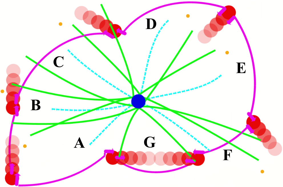
Figure 1: Visualization of gaps and trajectories generated by dynamic gap. The central blue dot represents the ego-robot while the red dots represent dynamic agents. Bolder dots denote the current agent poses while the more transparent dots denote future agent poses. Magenta arcs represent the instantaneous gaps obtained during Gap Detection (Section III-A1), and magenta arrows represent the gap state estimates (Section III-A3). Orange points represent the local gap goals, and green lines represent the Bézier curves that define the navigable gaps - labeled A-G in the figure - used during trajectory synthesis (Section III-C2). Dashed blue lines running through the navigable gaps labeled A-F represent the candidate trajectories generated at the current time step (Section III-C4). During the Gap Feasibility Analysis step (Section III-B), Gap G is deemed infeasible, resulting in the gap being discarded prior to trajectory synthesis.

This paper details an extension to prior work on the potential gap planner [8], involving augmentations to the planning framework to provide formal guarantees for safe navigation in dynamic environments. This extension is referred to hereafter as the dynamic gap local planner and can be visualized in Figure 1. Egocentric free space tracking is integrated to develop predictions of how gaps will evolve over time. These gap predictions along with known kinematic constraints are used to ensure that the defined workspace will remain as free space throughout the entire local time horizon. The employment of this safe workspace in junction with collision-free trajectory generation methods provides formal safety guarantees in ideal settings. For this work, ideal settings involve isolated gaps (no overlap between gaps during the local time horizon), and a first-order, point-mass, holonomic robot.

II Related Work

II-A Motion Planning in Dynamic Environments

Methods for tracking and predicting dynamic obstacles can be categorized into two approaches: model-based and motion-based. Model-based methods involve classifying obstacles from a predefined set of categories such as pedestrians or automobiles. This usually involves visual inferencing from a learned classifier [9]. Model-based methods are advantageous in that prediction models can be catered towards specific behaviors or classes [10], and they can identify objects in the scene that may not currently be moving but could move in the future. However, these approaches usually require a high level of confidence in the object classifier.

Motion-based methods involve detecting dynamic obstacles from sensor-derived motion cues. Gap-based planners fall into this category. These methods are advantageous in that they will capture any moving artifact in the environment, but they are disadvantageous in that they model all artifacts identically. To make obstacle predictions, motion-based methods perform data clustering, data association, and data estimation. Data clustering involves grouping input data into individual obstacles or subsections of obstacles. Data association involves finding pairings of clusters between consecutive time steps. The most common method is to treat this step as a Rectangular Assignment problem and solve via the Hungarian Algorithm [11]. Other methods may be used that are better suited for the problem domain [12]. Data estimation involves updating prediction models of the dynamic obstacles. Obstacles can be geometrically modeled in various ways: polygons or lines [13], circles [14, 15], or sets of points [16]. Prediction models can be factored into planning decisions through capturing them in cost functions or constraints in MPC formulations [17, 13], or embedding them in occupancy maps that can be searched over for paths [18, 19]. The methods cited here assign prediction models to individual obstacles and represent these prediction models with respect to a fixed frame. Performing obstacle tracking in the egocentric frame allows the local planner to leverage the benefits of operating in the perception space.

II-B Perception Space and Gap-based Navigation

A perception-space approach to planning involves keeping sensory input in its raw egocentric form to take advantage of the computational benefits that come with foregoing intensive data processing. All local planning steps downstream are then performed through an egocentric point of view. Prior work from the authors has been done to develop a hierarchical perception-space navigation stack. Specifically, efforts have been made towards efficient collision checking [20], egocentric environment representations [21], and local path planning [22, 8]. This hierarchical egocentric navigation stack, including the contributions highlighted in this work, can be seen in Figure 2.

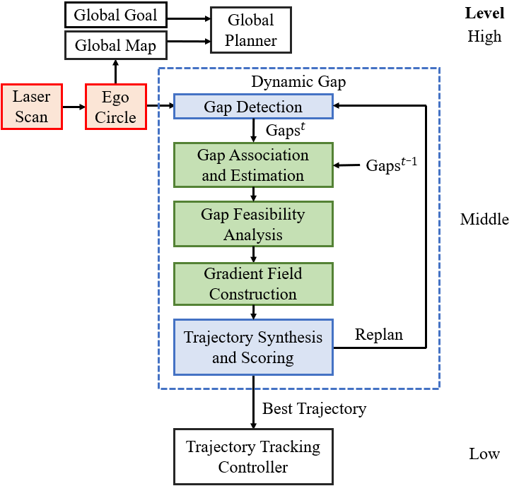
Figure 2: Information flow for egocentric hierarchical navigation stack, including dynamic gap as the local planner. Red boxes represent input perception data, blue boxes represent steps maintained from potential gap, and green boxes represent novel steps that were either added or augmented.

Gap-based planners typically function by operating on 1D laser scans and generating egocentric gaps: regions of collision-free space defined by either leading or trailing edges of obstacles. These planners either synthesize local trajectories or reactive control inputs through these gaps [3, 1, 7, 5, 4]. Potential Gap explored how to simplify and manipulate gap representations to uphold collision-free gap passage guarantees for manually-crafted artificial potential fields. To the authors’ knowledge, there are no gap-based planners in the literature that are explicitly designed to operate within dynamic environments.

II-C Artificial Harmonic Potential Fields

Artificial Potential Fields (APFs) are motion planning methods that obtain control inputs from the gradient of a potential function that returns higher values closer to obstacles and lower values closer to the goal [23, 24]. APFs encapsulate both safety and goal convergence through fast and simple means, but a major drawback of APFs is their tendency to have local minima due to complex world geometries. Many innovations have been made to alleviate such issues, one being Artificial Harmonic Potential Fields (AHPFs) which by design exhibit no local minima within a specified workspace [25, 26]. This is due to the fact that the critical points of a harmonic function strictly occur at saddle points, meaning that the robot may momentarily exist at these points but it will not settle at them. Recent work has explored algorithms that provide AHPFs for safe navigation in unknown workspaces by constraining the resultant vector field to point into the workspace at discrete points along the workspace boundary. [27]. It has been proven that assuming sufficient discretization, the resultant vector field will point inwards along the entire boundary, guaranteeing collision-free convergence to the goal position [28].

III Dynamic Gap Local Planning Module

This section details the approach that the proposed work takes to planning through feasible dynamic gaps. By virtue of the reachability-informed workspace, the resultant vector field guarantees safe gap passage under ideal conditions.

III-A Gap Detection, Association, and Estimation

III-A1 Gap Detection and Simplification

Potential gap defines a gap detection policy that operates on incoming egocircle [22] data to detect the instantaneous static gaps in the local environment. Gaps can either be classified as radial, in which there is a significant instantaneous change in range between consecutive scan points, or swept, in which there is a significant span of scan indices with maximum range values. Gap detection involves merging radial gaps into swept gaps, the latter of which possess favorable properties for planning such as high line-of-sight visibility. Dynamic gap adopts these detection and simplification policies, ultimately yielding a set of simplified gaps, $\mathcal{G}_{\rm simp}$.

III-A2 Gap Association

In static environments, solely gap detection is required for safe navigation, but association is now needed to understand how gaps evolve over time.

Each gap $G\in\mathcal{G}_{\rm simp}$ is comprised of a left and right point $p_{l},p_{r}\in\mathbb{R}^{2}$. Association is performed on the left and right points of the simplified gaps, this set can be referred to as $P_{\rm simp}$. The association step is represented as a rectangular assignment problem, where the cost is equivalent to the distance between points across consecutive steps, $P_{\rm simp}^{t-1}$ and $P_{\rm simp}^{t}$. This assignment problem is then solved with the Hungarian Algorithm, producing a minimum distance one-to-one mapping between $P_{\rm simp}^{t-1}$ and $P_{\rm simp}^{t}$. This association determines which points to transition models from and to across consecutive time steps. If the distance between two associated points exceeds a threshold $\tau_{assoc}$, then that point-to-point association is discarded.

III-A3 Gap Estimation

Given the desire to perform gap estimation in the perception space, the prediction models must represent the gap points with respect to the local robot frame which is constantly changing. Therefore, the constant velocity dynamics model taken with respect to the inertial frame is augmented to allow for translations and rotations of the robot. The state vector is defined as:

$$\textbf{X}=\begin{bmatrix}p_{s/b}\\ v_{s/b}\\ \end{bmatrix}=\begin{bmatrix}p_{s}-p_{b}\\ v_{s}-v_{b}\end{bmatrix},$$ (1)

where $p_{s/b}$ and $v_{s/b}$ represent the two-dimensional position and velocity of the gap side $s$ (left or right) relative to the robot body $b$, respectively. The system dynamics are then:

$$\dot{\textbf{X}}=\begin{bmatrix}\dot{p}_{s/b}\\ \dot{v}_{s/b}\\ \end{bmatrix}=\begin{bmatrix}v_{s/b}-\omega_{b}\times p_{s/b}\\ -a_{b}-\omega_{b}\times v_{s/b}\\ \end{bmatrix},$$ (2)

where $\omega_{b}$ represents the angular velocity of the robot and $a_{b}$ represents the linear acceleration of the robot. All values used for the estimator are represented in the body frame.

III-B Gap Feasibility Analysis

Within static environments, gap feasibility solely depends on whether or not the gap is wide enough to fit the robot. For dynamic environments, additional considerations must be made to determine whether or not the robot can pass through the gap before the gap shuts. By pruning away infeasible gaps, this step not only conserves energy of the robot, but it also avoids potentially dangerous gaps through which it would be difficult, if not impossible, for the robot to pass.

In order to remove the ego-robot motion from the gap state and solely analyze the motion of the gap itself, the gap-only dynamics are recovered from the prediction models by adding the robot’s ego-velocity $v_{b}$ to the relative velocity estimate $v_{s/b}$ to obtain the gap-only velocity $v_{s}$.

III-B1 Gap Categorization

Gap points can be categorized as static, expanding, or shrinking depending on their side, left or right, and their bearing rate of change, $\dot{\beta}$:

$$\text{Category}=\begin{cases}\text{Static}&\text{if $\dot{\beta}_{l}=0$ (or $\dot{\beta}_{r}=0$)}\\ \text{Expanding}&\text{if $\dot{\beta}_{l}>0$ (or $\dot{\beta}_{r}<0$)},\\ \text{Shrinking}&\text{if $\dot{\beta}_{l}<0$ (or $\dot{\beta}_{r}>0$)}\end{cases}$$ (3)

where $\dot{\beta}$ can be calculated as follows:

$$\dot{\beta}_{s}=\frac{p_{s,x}v_{s,y}-p_{s,y}v_{s,x}}{p_{s,x}^{2}+p_{s,y}^{2}}.$$ (4)

Gaps themselves can also be placed into the same categories depending on the overall rate of change of the gap angle. Define the angular size of gap $G\in\mathcal{G}_{\rm simp}$ as $\alpha$. Then:

$$\text{Category}=\begin{cases}\text{Static}&\text{if $\dot{\alpha}=0$}\\ \text{Expanding}&\text{if $\dot{\alpha}>0$}\\ \text{Shrinking}&\text{if $\dot{\alpha}<0$}\end{cases},$$ (5)

where $\dot{\alpha}=\dot{\beta_{l}}-\dot{\beta_{r}}$. Shrinking gaps are the only category that can be deemed infeasible given that they are the only category in which the gap can shut, signified by the left and right bearings crossing one another. Determining at what time this crossing occurs dictates whether or not the gap is kinematically feasible for the robot.

III-B2 Gap Propagation

Gap models are integrated forward for a local time horizon $T$ to determine the terminal gap points. Gap points can terminate prior to the end of the time horizon in two ways: if the gap closes, or if an expanding gap point becomes reachable. If neither of these conditions apply nor occur, the terminal points are set to the propagated points at the end of the time horizon.

At each time step $t$ during integration, a crossing condition is checked. A bearing crossing is interpreted as the clockwise angle of the gap switching from convex to non-convex when both the left and right bearings pass across the center of the gap. The clockwise angle condition is evaluated as:

$$(\alpha^{t-1}_{cw}>0)\wedge(\alpha^{t}_{cw}<0),$$ (6)

where

$$\alpha^{t}_{cw}=\arctan(\frac{\eta^{t}_{l}\cdot\eta^{t}_{r}}{\eta^{t}_{l}\times\eta^{t}_{r}}),$$ (7)

and the unit bearing vector for the gap sides at time $t$, $\eta_{s}^{t}$, is defined as:

$$\eta_{s}^{t}=\frac{\langle p_{s,x}^{t},p_{s,y}^{t}\rangle}{\lVert p_{s}^{t}\rVert}.$$ (8)

The condition for both bearings passing across the gap center is evaluated as:

$$(\eta^{t}_{l}\cdot\eta^{t-1}_{c}>0)\wedge(\eta^{t}_{l}\cdot\eta^{t-1}_{c}>0),$$ (9)

where $\eta_{c}^{t}$ refers to the unit bearing vector of the gap center. The crossing condition is visualized in Figure 3.

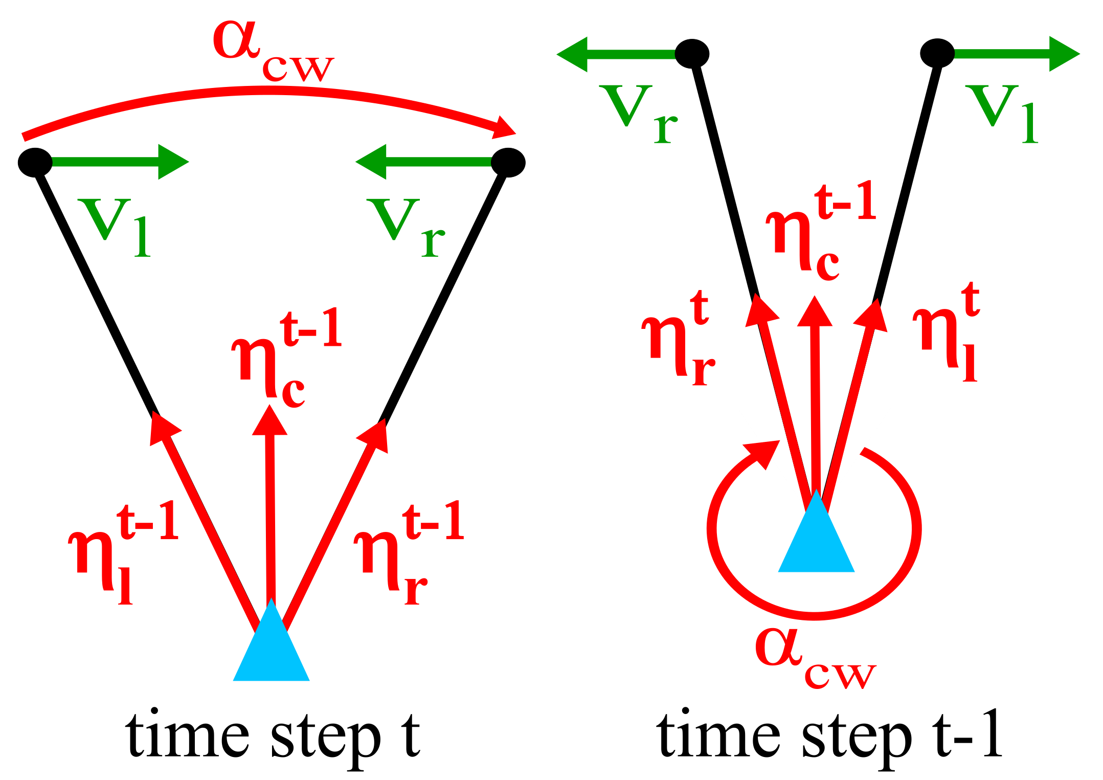
Figure 3: Crossing condition of a gap. At time step $t-1$, the left and right sides of the gap have yet to cross. At time step $t$, the gap sides have crossed, as shown by the clockwise angle and gap center conditions.

In the case that the gap bearings have crossed, a further evaluation is required to check if the gap has closed. For this, a range proximity condition is checked:

$$\lVert p_{l}^{t}-p_{r}^{t}\rVert<2r_{\rm infl},$$ (10)

where $r_{\rm infl}$ is the inflated radius of the robot. If the left and right points are sufficiently close together at the crossing, then the gap is closed. If a gap is deemed closed, the last time step at which the robot can fit between the gap points is used to set the terminal gap points.

The second terminal condition, for when expanding gap points first become reachable, is used to preserve the collision-free property of the gap. By terminating expanding gap points when they become reachable, it is ensured that no part of the gap point’s future trajectory that is reachable will overlap with the gap, therefore guaranteeing that the gap is a collision-free space. This condition is evaluated as:

$$\lVert p_{s}^{t}\rVert<v_{\rm max}t,$$ (11)

where $v_{\rm max}$ is the maximum linear velocity of the robot. This is a strict notion of reachability, assuming that the robot will travel in a straight line at its maximum velocity to intersect with the gap point’s trajectory.

III-B3 Gap Feasibility Testing

Once the initial and terminal gap points are set, a trajectory can be approximated to determine if it is feasible for the robot to pass through the gap during the local time horizon. This trajectory is estimated using a cubic spline that is constructed from the initial and terminal conditions of the robot and gap. If the maximum velocity along the spline does not exceed the linear velocity constraints of the robot, then the gap is deemed feasible. This feasibility analysis returns a set of gaps, $\mathcal{G}_{\rm feas}$, in which candidate trajectories will be synthesized.

III-C Gradient Field Construction

III-C1 Gap Manipulation

Potential gap applies manipulation steps to the gaps in $\mathcal{G}_{\rm simp}$ to ensure required gap properties for guaranteeing collision-free passage such as convexity. However, the trajectory synthesis method used in this work [27] assumes an unknown workspace and only requires that the boundary can be defined by a set of continuously differentiable functions. Therefore, the only manipulation step required is to inflate the gap boundary.

In static environments, it is only required to inflate a gap angularly to account for the radius of the robot. However, in dynamic environments, it is also required to inflate gaps outwards radially. Gaps may be attached to moving agents, so inflating the points outwards ensures that gap passage is synonymous with the robot moving completely beyond any agents potentially attached to the gap. This manipulation step yields a set of gaps $\mathcal{G}_{\rm manip}$ that are suitable for use in trajectory synthesis.

III-C2 Navigable Gap Construction

When planning in static environments, all free space within each gap $G\in\mathcal{G}_{\rm manip}$ is navigable given that $G$ persists without change for all time. However, we must now consider what subset of the gap is reachable at each future time step. To factor in this aspect, the left and right sides of the navigable gaps are modeled as weighted Bézier curves:

$$B_{s}(u)=(1-u^{2})O+2u(1-u)w_{s}^{0}p_{s}^{0}+u^{2}p_{s}^{1},u\in[0,1],$$ (12)

where $O\in\mathbb{R}^{2}$ is the origin of the Bézier curve, $p_{s}^{0},p_{s}^{1}\in\mathbb{R}^{2}$ are the initial and terminal gap points of $G$, and $u$ is the sliding variable used to parameterize the Bézier curve. A weight $w^{0}_{s}$ is applied to the initial gap point and set to $w_{s}^{0}=\lVert v_{s}\rVert/\lVert v_{\rm max}\rVert$. This weighting term works to lessen the curvature of the Bézier curve, making the gap easier to pass through while still respecting the gap dynamics.

III-C3 Gap Goal Placement

Navigable gap goals are placed within the angular span of the terminal gap bearings. For closing gaps, goals are placed beyond the point at which the gap points cross each other. For gaps that cross but do not close, goals are placed between the crossing points. Otherwise, goal placement is biased towards a navigation waypoint taken from the global plan.

III-C4 Artificial Harmonic Potential Field Construction

Dynamic environments can produce non-convex and unfavorable gap geometries in which it is difficult to guarantee robustness for a manually designed gradient field. To address this issue, we opt to leverage methods of automatically synthesizing artificial harmonic potential fields online which provide collision-free convergence guarantees. The involved trajectory synthesis method will be briefly explained below, and more implementation details can be found at [27].

Harmonic function terms are centered at $K$ discrete points along the weighted Bézier curves with one additional term placed at the reachable gap goal, which will be denoted as $p_{0}$. These harmonic terms take the form of

$$v_{k}(p;p_{k})=\ln(\lVert p-p_{k}\rVert),$$ (13)

where $p\in\mathbb{R}^{2}$ is the point within the workspace at which the term is evaluated and $p_{k}\in\mathbb{R}^{2}$ is the point at which the term is centered. The potential function $\Phi(p;p_{C}):\mathbb{R}^{2\times K+1}\rightarrow\mathbb{R}^{2}$ is constructed by taking a linear weighted combination of these harmonic terms:

$$\Phi(p;p_{C})=w^{T}v(p;p_{C}),$$ (14)

where $p_{C}\in\mathbb{R}^{2\times K+1}$ represents the vector of harmonic term centers and $w\in\mathbb{R}^{K+1}$ is a vector of weights applied to the harmonic terms. The weights are obtained by solving a Quadratic Program that minimizes $\lVert w\rVert$ while enforcing an inward-pointing vector field at the discrete points along the boundary. The linear velocity commands obtained from the vector field are then

$$u(p)=-||p-p_{0}||^{2}\nabla\Phi(p;p_{C}).$$ (15)

An example navigable gap along with its corresponding AHPF is shown in Figure 4.

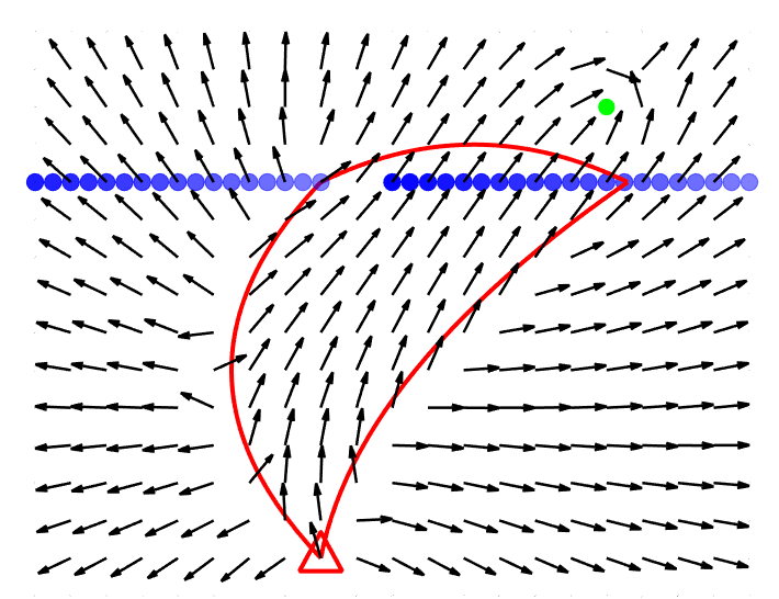
Figure 4: Example navigable gap and AHPF. The blue points correspond to the trajectory of the left and right gap points, with the fading of the points corresponding to the gap evolving over time.

Through this parameterization of the gap, collision-free convergence to the gap goal is guaranteed.

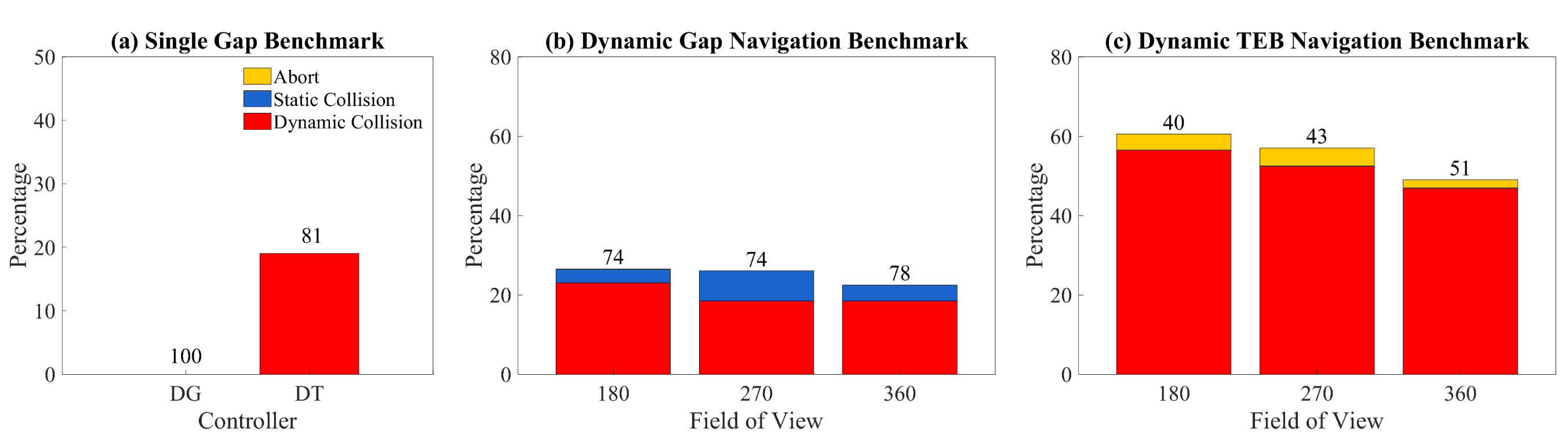
Figure 5: Collision percentage of dynamic gap (DG) and dynamic TEB (DT) vs. field of view. Single gap benchmarks are shown in subplot (a). Navigation benchmark performance along with observed failure modes for dynamic gap and dynamic TEB are shown in subplots (b) and (c) respectively.

III-C5 Proof of Collision-Free Passage

Assumptions made include an isolated, feasible gap characterized by constant velocity points, an ideal robot (first-order, point-mass, holonomic), and sufficient discretization of the gap boundary.

First, it will be shown that the navigable gap is comprised solely of free space over the local time horizon. This can be done by proving each gap side category separately. For static gap sides, this is trivial given that the gap side does not evolve over time. For closing gap sides, the Bézier curve divides the inside of the curve from the line segment between the two control points that represent the gap point trajectory. Therefore, the entire gap point trajectory lies outside of the navigable gap. For opening gap sides, if the terminal gap point is not reachable by the robot, then no part of the gap point trajectory is at risk of collision. If the terminal gap point is set to the first reachable point along the gap point’s trajectory, gap inflation prevents this point from leading to a collision. Therefore, the entire navigable gap is collision-free during the local time horizon.

Next, it will be shown that the resultant vector field generates collision-free trajectories. Prior work demonstrates that the employed AHPF guarantees safety over the entire boundary of the workspace as long as the workspace boundary is discretized with a sufficient number of points [28]. The minimum number of points required, $N_{0}$ can be found from an inequality derived from a Taylor Series expansion of the curves that define the workspace boundary. This inequality is detailed in the Theorem 1 of [28]. We implemented this inequality on the gaps used in this work and found that $N_{0}$ typically falls on the range of $[10,15]$. In implementation, the discrete number of points is set to $N=25$ to avoid the computation of repeatedly evaluating this inequality, and this is assumed to be sufficient discretization.

Finally, it must also be shown for closing gaps that the robot reaches the goal prior to the gap shutting. Since the gap is assumed to be feasible, there exists a feasible timescale that can be applied to the synthesized trajectory to ensure that the robot passes the gap before it closes.

III-D Trajectory Synthesis, Scoring, and Switching

III-D1 Trajectory Synthesis

In practice, the raw signal obtained from the AHPF was found to be small in magnitude, so the resulant velocities are scaled to provide a reasonable control signal. Forward integration is then performed on the resulting AHPFs for the local time horizon $T$ to obtain a set of candidate trajectories.

III-D2 Trajectory Scoring

Trajectories are scored in a similar manner as potential gap: based on their proximity to obstacles and their distance from the desired direction to the goal. A trajectory cost is comprised of a cumulative egocentric pose-wise cost based on the proximity to the current egocircle and a terminal pose cost based on proximity to a waypoint obtained from the global plan. In order to account for the evolution of the egocircle during the execution of the candidate trajectory, the odometries of dynamic agents are forward propagated and the egocircle is augmented accordingly. The highest-scoring candidate trajectory is compared to the currently executing trajectory to determine if a trajectory change should occur, as detailed in the next section.

III-D3 Trajectory Switching

The core idea behind safe hierarchical planners involves chaining together multiple safe local trajectories. Therefore, a method of triggering a switch to a newly synthesized local trajectory must be defined. Local trajectory switching is performed if the currently executing trajectory is deemed unsafe (either due to a future collision or due to the current gap being deemed infeasible), if the currently executing trajectory has ended, or if the prediction models that characterize the currently executing gap have been discarded during the gap point association step. If any of these situations arise, a switch to the highest-scoring candidate trajectory is triggered. If there are no valid candidate trajectories to switch to, then an obstacle avoidance policy is enacted until a candidate trajectory is synthesized.

IV Experiments and Outcomes

This section details the experiments performed between the proposed dynamic gap planner and the state-of-the-art Timed-Elastic-Bands (TEB) planner [13], which includes an extension for handling dynamic obstacles [29]. This extension performs blob detection on the fixed frame local costmap to identify obstacles and employs constant velocity Cartesian Kalman filters for tracking.

First, single gap benchmarks were performed in the Simple Two-Dimensional Robot (STDR) simulator [30] to confirm the collision-free properties that dynamic gap provides. Pairs of agents are randomly assigned a gap category (static, shrinking, or expanding) along with a speed (0.15, 0.30, or 0.45 m/s). Agent pairs are then spawned in an empty world with the ego-robot, and the ego-robot is to pass through the gap. This set up is meant to closely recreate the ideal settings under which the proof of collision-free gap passage is given. 100 trials were run for both dynamic gap and dynamic TEB, and the results are shown in subplot (a) of Figure 5. As expected, zero collisions were observed for dynamic gap whereas 19 were observed for dynamic TEB.

Second, navigation benchmarks are also run in STDR. Random unknown obstacles, both static and dynamic, are spawned throughout the world. Dynamic agents are given random start and goal poses along with a simple global path tracking controller. Four benchmarking worlds are utilized: the Dense, Campus, Office, and Sector worlds. The Campus and Office worlds can be seen in Figure 6. An agent density of 0.035 $\mathrm{agents/m^{2}}$ of free space is used in an attempt to normalize the difficulty of navigation across the worlds. Depending on the map size, this density yielded $16-74$ agents in total. The navigation planners are also tested at three fields of view: $180\degree,270\degree,$ and $360\degree$. Each setting is run with 50 unique random initial seeds in each world. Experiments are run on an Intel Core i7 processor.

Subplots (b) and (c) in Figure 5 provide the results of dynamic gap and dynamic TEB respectively along with a breakdown of the failure modes observed. These modes include aborts when the planner fails to find a realizable path to the goal, collisions with static artifacts in the environment such as walls or scattered obstacles, and collisions with the dynamic agents. Despite these benchmarks violating the assumptions for collision-free gap passage, the underlying framework of dynamic gap still leads the planner to outperform TEB by roughly 30% across the three fields of view tested. TEB leverages a soft-constraint time-optimal approach to local path planning. Therefore, no guarantees for collision avoidance can be made. This factor contributes significantly to the high collision rates observed for TEB. A majority of the collisions observed across both planners were due to collisions with the dynamic agents. A small number of the dynamic gap runs resulted in collisions with the static environment, but no runs result in an abort. Dynamic TEB shows the opposite trend, with some runs ending in an abort, but no runs resulting in static collisions.

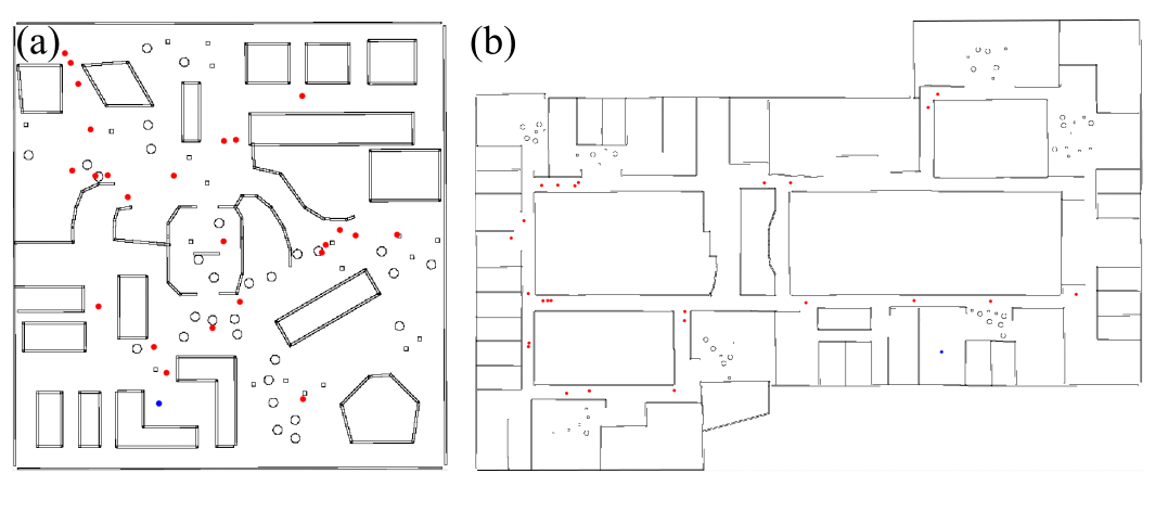
Figure 6: Campus (left) and Office (right) World in STDR simulator, with dynamic agents (red) and ego-robot (blue).

V Conclusion

This paper proposes an extension to an existent egocentric hierarchical navigation stack which involves adapting local gap-based planners to dynamic environments. This is accomplished through tracking the free space evolution relative to the egocentric frame, constructing collision-free navigable gaps based on gap dynamics and robot reachability, and synthesizing collision-free trajectories through Artificial Harmonic Potential Field methods. Navigation benchmarks showcase that the proposed work outperforms a state-of-the-art local planner that is also extended to dynamic environments. This code is open-sourced as a ROS package [31].

This work investigates methods of ensuring formal guarantees for safe navigation regarding trajectory generation for gap-based planners in dynamic environments. Future work will involve extending this framework to additionally provide formal guarantees for online trajectory execution as well as non-ideal robot dynamics such as nonholonomic or legged systems through the utilization of barrier functions.

References

- [1] M. Mujahad, D. Fischer, B. Mertsching, and H. Jaddu, “Closest gap based (cg) reactive obstacle avoidance navigation for highly cluttered environments,” in 2010 IEEE/RSJ International Conference on Intelligent Robots and Systems, 2010, pp. 1805–1812.
- [2] J. J. Gibson, The Ecological Approach to Visual Perception. Boston: Houghton Mifflin, 1979.
- [3] V. Sezer and M. Gokasan, “A novel obstacle avoidance algorithm: “follow the gap method”,” Robotics and Autonomous Systems, vol. 60, no. 9, pp. 1123–1134, 2012.
- [4] M. Mujahed and B. Mertsching, “The admissible gap (ag) method for reactive collision avoidance,” in 2017 IEEE International Conference on Robotics and Automation (ICRA), 2017, pp. 1916–1921.
- [5] M. Mujahed, D. Fischer, and B. Mertsching, “Safe gap based (sg) reactive navigation for mobile robots,” in 2013 European Conference on Mobile Robots, 2013, pp. 325–330.
- [6] M. Mujahed and B. Mertsching, “A new gap-based collision avoidance method for mobile robots,” in 2016 IEEE International Symposium on Safety, Security, and Rescue Robotics (SSRR), 2016, pp. 220–226.
- [7] M. Mujahed, H. Jaddu, D. Fischer, and B. Mertsching, “Tangential closest gap based (tcg) reactive obstacle avoidance navigation for cluttered environments,” in 2013 IEEE International Symposium on Safety, Security, and Rescue Robotics (SSRR), 2013, pp. 1–6.
- [8] R. Xu, S. Feng, and P. A. Vela, “Potential gap: A gap-informed reactive policy for safe hierarchical navigation,” IEEE Robotics and Automation Letters, vol. 6, no. 4, pp. 8325–8332, 2021.
- [9] T. Salzmann, B. Ivanovic, P. Chakravarty, and M. Pavone, Trajectron++: Dynamically-Feasible Trajectory Forecasting with Heterogeneous Data, 12 2020, pp. 683–700.
- [10] L. Zhao and C. Thorpe, “Qualitative and quantitative car tracking from a range image sequence,” in Proceedings. 1998 IEEE Computer Society Conference on Computer Vision and Pattern Recognition (Cat. No.98CB36231), 1998, pp. 496–501.
- [11] H. W. Kuhn, “The hungarian method for the assignment problem,” Naval Research Logistics Quarterly, vol. 2, no. 1-2, pp. 83–97, 1955.
- [12] D. Z. Wang, I. Posner, and P. Newman, “Model-free detection and tracking of dynamic objects with 2d lidar,” The International Journal of Robotics Research, vol. 34, no. 7, pp. 1039–1063, 2015.
- [13] C. Rösmann, F. Hoffmann, and T. Bertram, “Timed-elastic-bands for time-optimal point-to-point nonlinear model predictive control,” in 2015 European Control Conference (ECC), 2015, pp. 3352–3357.
- [14] P. Fiorini and Z. Shiller, “Motion planning in dynamic environments using the relative velocity paradigm,” in [1993] Proceedings IEEE International Conference on Robotics and Automation, 1993, pp. 560–565 vol.1.
- [15] J. van den Berg, M. Lin, and D. Manocha, “Reciprocal velocity obstacles for real-time multi-agent navigation,” in 2008 IEEE International Conference on Robotics and Automation, 2008, pp. 1928–1935.
- [16] S. Vaskov, S. Kousik, H. Larson, F. Bu, J. Ward, S. Worrall, M. Johnson-Roberson, and R. Vasudevan, “Towards provably not-at-fault control of autonomous robots in arbitrary dynamic environments,” 02 2019.
- [17] M. Gaertner, M. Bjelonic, F. Farshidian, and M. Hutter, “Collision-free mpc for legged robots in static and dynamic scenes,” 2021-04, p. 1550.
- [18] R. Senanayake, L. Ott, S. O' Callaghan, and F. T. Ramos, “Spatio-temporal hilbert maps for continuous occupancy representation in dynamic environments,” in Advances in Neural Information Processing Systems, D. Lee, M. Sugiyama, U. Luxburg, I. Guyon, and R. Garnett, Eds., vol. 29. Curran Associates, Inc., 2016.
- [19] V. Guizilini, R. Senanayake, and F. Ramos, “Dynamic hilbert maps: Real-time occupancy predictions in changing environments,” in 2019 IEEE International Conference on Robotics and Automation (ICRA), 2019, pp. 4091–4097.
- [20] J. S. Smith and P. Vela, “Pips: Planning in perception space,” in 2017 IEEE International Conference on Robotics and Automation (ICRA), 2017, pp. 6204–6209.
- [21] J. S. Smith, S. Feng, F. Lyu, and P. A. Vela, Real-Time Egocentric Navigation Using 3D Sensing. Cham: Springer International Publishing, 2020, pp. 431–484.
- [22] J. S. Smith, R. Xu, and P. Vela, “egoteb: Egocentric, perception space navigation using timed-elastic-bands,” in 2020 IEEE International Conference on Robotics and Automation (ICRA), 2020, pp. 2703–2709.
- [23] D. Koditschek, “Exact robot navigation by means of potential functions: Some topological considerations,” in Proceedings. 1987 IEEE International Conference on Robotics and Automation, vol. 4, 1987, pp. 1–6.
- [24] O. Khatib, “Real-time obstacle avoidance for manipulators and mobile robots,” in Proceedings. 1985 IEEE International Conference on Robotics and Automation, vol. 2, 1985, pp. 500–505.
- [25] J.-O. Kim and P. Khosla, “Real-time obstacle avoidance using harmonic potential functions,” IEEE Transactions on Robotics and Automation, vol. 8, no. 3, pp. 338–349, 1992.
- [26] S. G. Loizou, “Closed form navigation functions based on harmonic potentials,” in 2011 50th IEEE Conference on Decision and Control and European Control Conference, 2011, pp. 6361–6366.
- [27] P. Rousseas, C. P. Bechlioulis, and K. J. Kyriakopoulos, “Trajectory planning in unknown 2d workspaces: A smooth, reactive, harmonics-based approach,” IEEE Robotics and Automation Letters, vol. 7, no. 2, pp. 1992–1999, 2022.
- [28] P. Rousseas, C. Bechlioulis, and K. J. Kyriakopoulos, “Harmonic-based optimal motion planning in constrained workspaces using reinforcement learning,” IEEE Robotics and Automation Letters, vol. 6, no. 2, pp. 2005–2011, 2021.
- [29] C. Rösmann, F. Hoffmann, and T. Bertram, “Track and include dynamic obstacles via costmap_converter,” 2018. [Online]. Available: http://wiki.ros.org/teb_local_planner
- [30] A. T. M. Tsardoulias and C. Zalidis, “stdr_simulator - ros_wiki,” 2014. [Online]. Available: http://wiki.ros.org/stdr_simulator
- [31] M. Asselmeier, Y. Zhao, and P. A. Vela, “Dynamic gap.” [Online]. Available: https://github.com/ivaROS/DynamicGap