The good, the bad and the ugly sides of data augmentation:
An implicit spectral regularization perspective

Abstract

Data augmentation (DA) is a powerful workhorse for bolstering performance in modern machine learning. Specific augmentations like translations and scaling in computer vision are traditionally believed to improve generalization by generating new (artificial) data from the same distribution. However, this traditional viewpoint does not explain the success of prevalent augmentations in modern machine learning (e.g. randomized masking, cutout, mixup), that greatly alter the training data distribution. In this work, we develop a new theoretical framework to characterize the impact of a general class of DA on underparameterized and overparameterized linear model generalization. Our framework reveals that DA induces implicit spectral regularization through a combination of two distinct effects: a) manipulating the relative proportion of eigenvalues of the data covariance matrix in a training-data-dependent manner, and b) uniformly boosting the entire spectrum of the data covariance matrix through ridge regression. These effects, when applied to popular augmentations, give rise to a wide variety of phenomena, including discrepancies in generalization between over-parameterized and under-parameterized regimes and differences between regression and classification tasks. Our framework highlights the nuanced and sometimes surprising impacts of DA on generalization, and serves as a testbed for novel augmentation design.

Keywords: Data augmentation, Generalization analysis, Overparameterized models, Spectral analysis, Regression, Classification

.tocmtchapter mtchapternone mtappendixnone

1 Introduction

Data augmentation (DA), or the transformation of data samples before or during learning, is quickly becoming a workhorse of both supervised (Shorten and Khoshgoftaar, 2019; Iosifidis and Ntoutsi, 2018; Liu et al., 2021b) and self-supervised approaches (Chen et al., 2020b; Grill et al., 2020; Azabou et al., 2021; Zbontar et al., 2021) for machine learning (ML). It is critical to the success of modern ML in multiple domains, e.g., computer vision (Shorten and Khoshgoftaar, 2019), natural language processing (Feng et al., 2021), time series data (Wen et al., 2020), and neuroscience (Lashgari et al., 2020; Azabou et al., 2021; Liu et al., 2021a). This is especially true in settings where data and/or labels are scarce or in other cases where algorithms are prone to overfitting (Zhang et al., 2021). While DA is perhaps one of the most widely used tools for regularization, most augmentations are often applied in an ad hoc manner, and it is often unclear exactly how, why, and when a DA strategy will work for a given dataset (Cubuk et al., 2019; Ratner et al., 2017).

Recent theoretical studies have provided insights into the effect of DA on learning and generalization when augmented samples lie close to the original data distribution (Dao et al., 2019; Chen et al., 2020a). However, state-of-the-art augmentations that are used in practice (e.g. data masking (He et al., 2022), cutout (DeVries and Taylor, 2017), mixup (Zhang et al., 2017)) are stochastic and can significantly alter the distribution of the data (Gontijo-Lopes et al., 2020; He et al., 2022; Yuan et al., 2021). Despite many efforts to explain the success of DA in the literature (Bishop, 1995; Chapelle et al., 2001; Chen et al., 2020a; Dao et al., 2019; Wu et al., 2020), there is still a lack of a comprehensive platform to compare different types of augmentations at a quantitative level.

In this paper, we address this challenge by proposing a simple yet flexible theoretical framework for comparing the linear model generalization of a broad class of augmentations. Our framework is simultaneously applicable to: 1. general stochastic augmentations, e.g. Chen et al. (2020a); Assran et al. (2022); DeVries and Taylor (2017); He et al. (2022), 2. the classical underparameterized regime (Hastie et al., 2009) and the modern overparameterized regime (Zhang et al., 2021; Belkin et al., 2019), 3. regression (Bartlett et al., 2020; Tsigler and Bartlett, 2020) and classification tasks (Muthukumar et al., 2021; Wang and Thrampoulidis, 2021), and 4. strong and weak distributional-shift augmentations (Yuan et al., 2021). To do this, we borrow and build on finite-sample analysis techniques of the modern overparameterized regime for linear and kernel models (Bartlett et al., 2020; Tsigler and Bartlett, 2020; Muthukumar et al., 2021, 2020). Our theory reveals that DA induces implicit, training-data-dependent regularization of a twofold type: a) manipulation of the spectrum (i.e. eigenvalues) of the data covariance matrix, and b) the addition of explicit $\ell_{2}$-type regularization to avoid noise overfitting.

The first effect of spectral manipulation is often dominant in the overparameterized regime, and we show through several examples how it can either make or break generalization by introducing helpful or harmful biases. In contrast, the explicit $\ell_{2}$ regularization effect always improves generalization by preventing possibly harmful overfitting of noise.

1.1 Main contributions

Below, we outline and provide a roadmap of the main contributions of this work.

• We propose a new framework for studying generalization with data augmentation for linear models by building on the recent literature on the theory of overparameterized learning (Bartlett et al., 2020; Belkin et al., 2020; Hastie et al., 2019; Muthukumar et al., 2020, 2021; Wang and Thrampoulidis, 2021). We provide natural definitions of the augmentation mean and covariance operators that capture the impact of change in data distribution on model generalization in Section 3.1, and sharply characterize the ensuing performance for both regression and classification tasks in Sections 4.3 and 4.4, respectively.

• In Section 5.1, we apply our theory to provide novel and surprising interpretations of a broad class of randomized DA strategies used in practice; e.g., random-masking (He et al., 2022), cutout (DeVries and Taylor, 2017), noise injection (Bishop, 1995), and group-invariant augmentations (Chen et al., 2020a). An example is as follows: while the classical noise injection augmentation (Bishop, 1995) causes only a constant shift in the spectrum, data masking (He et al., 2022; Assran et al., 2022), cutout (DeVries and Taylor, 2017) and distribution-preserving augmentations (Chen et al., 2020a) tend to isotropize the equivalent data spectrum. This isotropizing effect, as we discuss in Section 5.2, can be shown to create an especially high bias and therefore, harm generalization in the overparameterized regime.

• In Section 5.3, we directly compare the impact of DA on the downstream tasks of regression and classification and identify strikingly different behaviors. Specifically, we find that, while augmentation bias is mostly harmful in a regression task, its effect can be minimal for classification. This together with the uniform variance improvement can be shown to yield several helpful scenarios for classification. This is consistent with the fact that the empirical benefits of strong augmentation have been observed primarily in classification tasks (Yuan et al., 2021; Dai et al., 2022).

• Our framework serves as a testbed for new DA approaches. As a proof-of-concept, in Section 5.2.2, we design a new augmentation method, inspired by isometries in random feature rotation, that can provably achieve smaller bias than the least-squared estimator and variance reduction on the order of the ridge estimator. Moreover, this generalization is robust in the sense that it compares favorably with optimally tuned ridge regression for a much wider range of hyperparameters.

• Finally, in Section 6 we complement and verify our theoretical insights through a number of empirical studies that examine how multiple factors involving data, model and augmentation type impact generalization. We compare our closed-form expression with augmented SGD (Dao et al., 2019; Chen et al., 2020a, b) and pre-computed augmentations (Wu et al., 2020; Shen et al., 2022). In contrast to augmented SGD, we find that adding more pre-computed augmentations can increase overfitting to noise, thus producing “interpolation peaks” in the sense of Belkin et al. (2019).

Notation

We use $n$ to denote the number of training examples and $p$ to denote the data dimension. Given a training data matrix $\mathbf{X}\in\mathbb{R}^{n\times p}$ where each row (representing a training example) is independently and identically distributed (i.i.d.) and has covariance ${\boldsymbol{\Sigma}}:=\mathbb{E}[\mathbf{x}\mathbf{x}^{\top}]$, we denote $\mathbf{P}^{{\boldsymbol{\Sigma}}}_{1:k-1}$ and $\mathbf{P}^{{\boldsymbol{\Sigma}}}_{k:\infty}$ as the projection matrices to the top $k-1$ and the bottom $p-k+1$ eigen-subspaces of ${\boldsymbol{\Sigma}}$, respectively. For convenience, we denote the residual Gram matrix by $\mathcal{A}_{k}(\mathbf{\mathbf{X}};\lambda)=\lambda\mathbf{I}_{n}+\mathbf{\mathbf{X}}\boldsymbol{P}^{{\boldsymbol{\Sigma}}}_{k:\infty}\mathbf{\mathbf{X}}^{T}$, where $\lambda$ is some regularization constant. Subscripts denote the subsets of column vectors when applied to a matrix; e.g. for a matrix $\mathbf{V}$ we have $\mathbf{V}_{a:b}:=[\mathbf{v}_{a},\mathbf{v}_{a+1},\dots,\mathbf{v}_{b}]$. A similar definition applies to vectors; e.g. for a vector $\mathbf{x}$ we have $\mathbf{\mathbf{x}}_{a:b}=[\mathbf{x}_{a},\mathbf{x}_{a+1},\dots,\mathbf{x}_{b}]$. The Mahalanobis norm of a vector is defined by $\|\mathbf{x}\|_{\mathbf{H}}=\sqrt{\mathbf{x}^{\top}\mathbf{H}\mathbf{x}}$. For a matrix $\mathbf{A}$, $\mathrm{diag}({\mathbf{A}})$ denotes the diagonal matrix with a diagonal equal to that of $\mathbf{A}$, $\mathrm{Tr}(\mathbf{A})$ denotes its trace and $\mu_{i}(\mathbf{A})$ its $i$-th largest eigenvalue. The symbols $\gtrsim$ and $\lesssim$ are used to denote inequality relations that hold up to universal constants that do not depend on $n$ or $p$. All asymptotic convergence results are stated in probability.

More specific notation corresponding to our signal model is given in Section 4.1, and some additional notation that is convenient to define for our analysis is postponed to Section 4.2.

2 Related work

We organize our discussion of related work into two verticals: a) historical and recent perspectives on the role of data augmentation, and b) recent analyses of minimum-norm and ridge estimators in the over-parameterized regime.

2.1 Data augmentation

Classical links between DA and regularization:

Early analysis of DA showed that adding random Gaussian noise to data points is equivalent to Tikhonov regularization (Bishop, 1995) and vicinal risk minimization (Zhang et al., 2017; Chapelle et al., 2001); in the latter, a local distribution is defined in the neighborhood of each training sample, and new samples are drawn from these local distributions to be used during training. These results established an early link between augmentation and explicit regularization. However, the impact of such approaches on generalization has been mostly studied in the underparameterized regime of ML, where the primary concern is reducing variance and avoiding overfitting of noise. Modern ML practices, by contrast, have achieved great empirical success in overparameterized settings and with a broader range of augmentation strategies (Shorten and Khoshgoftaar, 2019; Iosifidis and Ntoutsi, 2018; Liu et al., 2021b). The type of regularization that is induced by these more general augmentation strategies is not well understood. Our work provides a systematic point of view to study this general connection without assuming any additional explicit regularization, or specific operating regime.

In-distribution versus out-of-distribution augmentations:

Intuitively, if we could design an augmentation that would produce more virtual but identically distributed samples of our data, we would expect an improvement in generalization. Based on this insight and the inherent structure of many augmentations used in vision (that have symmetries), another set of works explores the common intuition that data augmentation helps insert beneficial group-invariances into the learning process (Cohen and Welling, 2016; Raj et al., 2017; Mroueh et al., 2015; Bruna and Mallat, 2013; Yang et al., 2019). These studies generally consider cases in which the group structure is explicitly present in the model design via convolutional architectures (Cohen and Welling, 2016; Bruna and Mallat, 2013) or feature maps approximating group-invariant kernels (Raj et al., 2017; Mroueh et al., 2015). The authors of Chen et al. (2020a) propose a general group-theoretic framework for DA and explain that an averaging effect helps the model generalize through variance reduction. However, they only consider augmentations that do not alter (or alter by minimal amounts) the original data distribution; consequently, they identify variance reduction as a sole positive effect of DA. Moreover, their analysis applies primarily to underparameterized or explicitly regularized models.

Recent empirical studies have highlighted the importance of diverse stochastic augmentations (Gontijo-Lopes et al., 2020). They argue that in many cases, it is important to introduce samples which are out-of-distribution (OOD) (Sinha et al., 2021; Peng et al., 2022) (in the sense that they do not resemble the original data). In our framework, we allow for cases in which augmentation leads to significant changes in distribution and provide a path to analysis for such OOD augmentations that encompass empirically popular approaches for DA (He et al., 2022; DeVries and Taylor, 2017). We also consider the modern overparameterized regime (Belkin et al., 2019; Dar et al., 2021). We show that the effects of OOD augmentations go far beyond variance reduction, and the spectral manipulation effect introduces interesting biases that can either improve or worsen generalization for overparameterized models.

Analysis of specific types of DA in linear and kernel methods:

Dao et al. (2019) propose a Markov process-based framework to model compositional DA and demonstrate an asymptotic connection between a Bayes-optimal classifier and a kernel classifier dependent on DA. Furthermore, they study the augmented empirical risk minimization procedure and show that some types of DA, implemented in this way, induce approximate data-dependent regularization. However, unlike our work, they do not quantitatively study the generalization of these classifiers. Li et al. (2019) also propose a kernel classifier based on a notion of invariance to local translations, which produces competitive empirical performance. In another recent analysis, Wu et al. (2020) study the generalization of linear models with DA that constitutes linear transformations on the data for regression in the overparameterized regime (but still considering additional explicit regularization). They find that data augmentation can enlarge the span of training data and induce regularization. There are several key differences between their framework and ours. First, they analyze deterministic DA, while we analyze stochastic augmentations used in practice (Grill et al., 2020; Chen et al., 2020a). Second, they assume that the augmentations would not change the labels generated by the ground-truth model, thereby only identifying beneficial scenarios for DA (while we identify scenarios that are both helpful and harmful). Third, they study empirical risk minimization with pre-computed augmentations, in contrast to our study of augmentations applied on-the-fly during the optimization process (Dao et al., 2019; Chen et al., 2020a), which are arguably more commonly used in practice. Our experiments in Section 6.4 identify sizably different impacts of these methods of application of DA even in simple linear models. Finally, the role of DA in linear model optimization, rather than generalization, has also been recently studied; in particular, Hanin and Sun (2021) characterize how DA affects the convergence rate of optimization.

The impact of DA on nonlinear models:

Recent works aim to to understand the role of DA in nonlinear models such as neural networks. LeJeune et al. (2019) show that certain local augmentations induce regularization in deep networks via a “rugosity”, or “roughness” complexity measure. While they show empirically that DA reduces rugosity, they leave open the question of whether this alone is an appropriate measure of a model’s generalization capability. Very recently, Shen et al. (2022) showed that training a two-layer convolutional neural network with a specific permutation-style augmentation can have a novel feature manipulation effect. Assuming the recently posited “multi-view" signal model (Allen-Zhu and Li, 2020), they show that this permutation-style DA enables the model to better learn the essential feature for a classification task. They also observe that the benefit becomes more pronounced for nonlinear models. Our work provides a similar message, as we also identify the DA-induced data manipulation effect as key to generalization. Because our focus in this work is limited to linear models, the effect of data manipulation manifests itself purely through spectral regularization of the data covariance. As a result of this spectral-regularization effect, we are also able to provide a comprehensive general-purpose framework for DA by which we can compare and contrast different augmentations that can either help or hurt generalization (while Shen et al. (2022) only analyze a permutation-style augmentation). We believe that combining our general-purpose framework for DA with a more complex nonlinear model analysis is a promising future direction, and we discuss possible analysis paths for this in Section 7.

2.2 Interpolation and regularization in overparameterized models

Minimum-norm-interpolation analysis:

Our technical approach leverages recent results in overparameterized linear regression, where models are allowed to interpolate the training data. Following the definition of Dar et al. (2021), we characterize such works by their explicit focus on models that achieve close to zero training loss and which have a high complexity relative to the number of training samples. Specifically, many of these works provide finite sample analysis of the risk of the least squared estimator (LSE) and the ridge estimator (Bartlett et al., 2020; Tsigler and Bartlett, 2020; Hastie et al., 2019; Belkin et al., 2020; Muthukumar et al., 2020). This line of research (most notably, Bartlett et al. (2020); Tsigler and Bartlett (2020)) finds that the mean squared error (MSE), comprising the bias and variance, can be characterized in terms of the effective ranks of the spectrum of the data distribution. The main insight is that, contrary to traditional wisdom, perfect interpolation of the data may not have a harmful effect on the generalization error in highly overparameterized models. In the context of these advances, we identify the principal impact of DA as spectral manipulation which directly modifies the effective ranks, thus either improving or worsening generalization. We build in particular on the work of Tsigler and Bartlett (2020), who provide non-asymptotic characterizations of generalization error for general sub-Gaussian design, with some additional technical assumptions that also carry over to our framework.

Subsequently, this type of “harmless interpolation” was shown to occur for classification tasks (Muthukumar et al., 2021; Cao et al., 2021; Wang and Thrampoulidis, 2021; Chatterji and Long, 2021; Shamir, 2022; Deng et al., 2022; Montanari et al., 2019). In particular, Muthukumar et al. (2021); Shamir (2022) showed that classification can be significantly easier than regression due to the relative benignness of the 0-1 test loss. Our analysis also compares classification and regression and shows that the potentially harmful biases generated by DA are frequently nullified with the 0-1 metric. As a result, we identify several beneficial scenarios for DA in classification tasks. At a technical level, we generalize the analysis of Muthukumar et al. (2021) to sub-Gaussian design. We also believe that our framework can be combined with the alternative mixture model (where covariates are generated from discrete labels (Chatterji and Long, 2021; Wang and Thrampoulidis, 2021; Cao et al., 2021)), but we do not formally explore this path in this paper.

Generalized $\ell_{2}$ regularizer analysis:

Our framework extends the analyses of least squares and ridge regression to estimators with general Tikhonov regularization, i.e., a penalty of the form $\theta^{\top}\mathbf{M}\theta$ for arbitrary positive definite matrix $\mathbf{M}$. A closely related work is Wu and Xu (2020), which analyzes the regression generalization error of general Tikhonov regularization. However, our work differs from theirs in three key respects. First, the analysis of Wu and Xu (2020) is based on the proportional asymptotic limit (where the sample size $n$ and data dimension $p$ increase proportionally with a fixed ratio) and provides sharp asymptotic formulas for regression error that are exact, but not closed-form and not easily interpretable. On the other hand, our framework is non-asymptotic, and we generally consider $p\gg n$ or $p\ll n$; our expressions are closed-form, match up to universal constants and are easily interpretable. Second, our analysis allows for a more general class of random regularizers that themselves depend on the training data; a key technical innovation involves showing that the additional effect of this randomness is, in fact, minimal. Third, we do not explicitly consider the problem of determining an optimal regularizer; instead, we compare and contrast the generalization characteristics of various types of practical augmentations and discuss which characteristics lead to favorable performance.

In addition to explicitly regularized estimators, Wu and Xu (2020) also analyze the ridgeless limit for these regularizers, which can be interpreted as the minimum-Mahalanobis-norm interpolator. In Section 6.1 we show that such estimators can also be realized in the limit of minimal DA.

The role of explicit regularization and hyperparameter tuning:

Research on harmless interpolation and double descent (Belkin et al., 2019) has challenged conventional thinking about regularization and overfitting for overparameterized models; in particular, good performance can be achieved with weak (or even negative) explicit regularization (Kobak et al., 2020; Tsigler and Bartlett, 2020), and gradient descent trained to interpolation can sometimes beat ridge regression (Richards et al., 2021). These results show that the scale of the ridge regularization significantly affects model generalization; consequently, recent work strives to estimate the optimal scale of ridge regularization using cross-validation techniques (Patil et al., 2021, 2022).

As shown in classical work (Bishop, 1995), ridge regularization is equivalent to augmentation with (isotropic) Gaussian noise, and the scale of regularization naturally maps to the variance of Gaussian noise augmentation. Our work links DA to a much more flexible class of regularizers and shows that some types of DA induce an implicit regularization that yields much more robust performance across the hyperparameter(s) dictating the “strength” of the augmentation. In particular, our experiments in Section 6.2 show that random mask (He et al., 2022), cutout (DeVries and Taylor, 2017) and our new random rotation augmentation yield comparable generalization error for a wide range of hyperparameters (masking probability, cutout width and rotation angle respectively); the random rotation is a new augmentation proposed in this work and frequently beats ridge regularization as well as interpolation. Thus, our flexible framework enables the discovery of DA with appealing robustness properties not present in the more basic methodology of ridge regularization.

Other types of indirect regularization:

We also mention peripherally related but important work on other types of indirect regularization involving creating fake “knockoff” features (Candes et al., 2018; Romano et al., 2020) and dropout in parameter space (Cavazza et al., 2018; Mianjy et al., 2018). The knockoff methodology creates copies of features (rather than augmenting data points) that are uncorrelated with the target to perform variable selection. Dropout also induces implicit regularization by randomly dropping out intermediate neurons (rather than covariates, as does the random mask (He et al., 2022) augmentation) during the learning process, and has been shown to have a close connection with sparsity regularization (Mianjy et al., 2018). Overall, these constitute methods of indirect regularization that are applied to model parameters rather than data. An intriguing question for future work is whether these effects can also be achieved through DA.

3 Problem Setup

In this section, we introduce the notation and setup for our analysis of generalization with data augmentation (DA). We review the fundamentals of empirical risk minimization (ERM) without DA and how augmentations affect the ERM procedure. Then, we derive a reduction to ridge regression that paves the way for our analysis in Section 4.

3.1 Empirical risk minimization with data augmentation

Modern, high-dimensional ML models are commonly trained to minimize a combination of a) prediction error on training data, and b) a measure of model complexity that favors “simpler" or “smaller" models. This is encapsulated in the regularized empirical risk minimization objective, expressed for linear models $f_{\boldsymbol{\theta}}(\mathbf{x})=\langle\mathbf{x},\boldsymbol{\theta}\rangle$ as

$$\hat{\boldsymbol{\theta}}=\arg\min_{{{\boldsymbol{\theta}}}}\leavevmode\nobreak\ \ell(\mathbf{X}\boldsymbol{\theta},\mathbf{y})+R({\boldsymbol{\theta}}),$$ (1)

where $\ell$ is a loss function, $\mathbf{X}=\begin{bmatrix}\mathbf{x}_{1}&\ldots&\mathbf{x}_{n}\end{bmatrix}^{\top}\in\mathbb{R}^{n\times p}$ is the training data matrix that stacks the $n$ covariates, $\mathbf{y}\in\mathbb{R}^{n}$ is the vector of observations/responses, $\boldsymbol{\theta}\in\mathbb{R}^{p}$ is the linear model parameter that we want to optimize, and $R(\boldsymbol{\theta})$ is an explicit regularizer applied to the model. For example, the popular ridge regression procedure uses $R(\boldsymbol{\theta};\lambda)=\lambda\|\boldsymbol{\theta}\|_{2}^{2}$, where $\lambda$ is a tunable hyperparameter. We will adopt the choice of squared loss function $\ell(\mathbf{X}\boldsymbol{\theta},\mathbf{y})=\|\mathbf{X}\boldsymbol{\theta}-\mathbf{y}\|_{2}^{2}$ throughout this work, owing to its mathematical tractability and recently observed competitiveness with the cross-entropy loss even in classification tasks (Hui and Belkin, 2020; Muthukumar et al., 2021; Wang and Thrampoulidis, 2021; Chatterji and Long, 2021).

Although the training objective of modern supervised ML models rarely includes explicit regularization of the form (1) in practice, it does heavily rely on data augmentation (DA) to achieve state-of-the-art performance (Shorten and Khoshgoftaar, 2019; Zhang et al., 2021). Mathematically speaking, an augmentation $g:\mathbb{R}^{p}\to\mathbb{R}^{p}$ is a general mapping from the original data point $\mathbf{x}$ to a transformed data point $g(\mathbf{x})$. In practice, an augmentation function $g$ is often stochastic and drawn at random from an augmentation distribution denoted by $\mathcal{G}$. Each time we augment the data, we randomly draw an instance of $g\sim\mathcal{G}$. For example, the classical Gaussian noise injection augmentation (Bishop, 1995) is stochastic and takes the form $g(\mathbf{x})=\mathbf{x}+\mathbf{n}$, where $\mathbf{n}$ is an isotropic Gaussian random variable.

One approach to implement augmentations is to pre-compute augmented data samples by drawing a fixed number of augmentations before training and then including them along with the original data points when training the model (Wu et al., 2020; Shen et al., 2022). Nowadays, it is more popular to apply augmentations on the fly during training (Chen et al., 2020a; Grill et al., 2020), with different transformations applied stochastically throughout the training procedure. This procedure, typically called augmented stochastic gradient descent (aSGD), is widely used in practice (Chen et al., 2020b, a). Chen et al. (2020a) showed that this algorithm can be viewed as applying SGD to the objective of an augmented empirical risk minimization (aERM) problem:

$$\hat{\boldsymbol{\theta}}=\arg\min_{\boldsymbol{\theta}}\mathbb{E}_{G}\left[\|G(\mathbf{X})\boldsymbol{\theta}-\mathbf{y}\|_{2}^{2}\right].$$ (2)

Above, $G$ denotes a stacked data augmentation function applied to each row of the matrix, i.e., $G(\mathbf{X})=[g_{1}(\mathbf{x}_{1})\dots,g_{n}(\mathbf{x}_{n})]^{T}$; we assume that the transformations $g_{i}$ are stochastic and are drawn i.i.d. from an augmentation function distribution $\mathcal{G}$. We would expect aSGD to converge to the solution of (2), and conduct experiments to empirically verify this in Section 6.

We begin by defining the first and second-order statistics of an augmentation distribution. We will show that these quantities play a key role in characterizing the solution to the aERM problem.

Definition 1 (Augmentation Mean and Covariance Operator).

Consider a stochastic augmentation $\mathbf{x}\mapsto g(\mathbf{x})$, where $g$ is drawn randomly from an augmentation distribution $\mathcal{G}$. We then define the augmentation mean and the covariance for a single data point $\mathbf{x}$ as

$$\mu_{\mathcal{G}}(\mathbf{x}):=\mathbb{E}_{g\sim\mathcal{G}}[g(\mathbf{x})],\leavevmode\nobreak\ \leavevmode\nobreak\ \mathrm{{Cov}}_{\mathcal{G}}(\mathbf{x}):=\mathbb{E}_{g\sim\mathcal{G}}\left[\left(g(\mathbf{x})-\mu_{\mathcal{G}}(\mathbf{x})\right)\left(g(\mathbf{x})-\mu_{\mathcal{G}}(\mathbf{x})\right)^{\top}\right],$$ (3)

where we use the subscript $\mathcal{G}$ to emphasize that the expectation is only over the randomness of the augmentation function $g$. Furthermore, for a training data set $\mathbf{X}=\begin{bmatrix}\mathbf{x}_{1}&\ldots&\mathbf{x}_{n}\end{bmatrix}^{\top}$, we similarly define the augmentation mean and covariance operators with respect to the data set as:

$$\mu_{\mathcal{G}}(\mathbf{X}):=[\mu_{\mathcal{G}}(\mathbf{x}_{1}),\mu_{\mathcal{G}}(\mathbf{x}_{2}),\dots,\mu_{\mathcal{G}}(\mathbf{x}_{n})]^{\top},\leavevmode\nobreak\ \leavevmode\nobreak\ \mathrm{{Cov}}_{\mathcal{G}}(\mathbf{X}):=\frac{1}{n}\sum_{i=1}^{n}\mathrm{{Cov}}_{\mathcal{G}}(\mathbf{x}_{i}).$$ (4)

Finally, we call an augmentation distribution unbiased on average if $\mu_{\mathcal{G}}(\mathbf{x})=\mathbf{x}$.

With this notation introduced, we now explain why DA gives rise to implicit regularization. For now we consider augmentation distributions that are unbiased on average for conceptual simplicity and leave the extension to distributions that are biased on average to Section 4.3.2. For such unbiased-on-average augmentation distributions, we can simply the objective (2) as:

$$\mathbb{E}_{G}[\|G(\mathbf{X})\boldsymbol{\theta}-\mathbf{y})\|_{2}^{2}] =\mathbb{E}_{G}[\|\left(G(\mathbf{X})-\mu(\mathbf{X})\right)\boldsymbol{\theta}+\mu(\mathbf{X})\boldsymbol{\theta}-\mathbf{y})\|_{2}^{2}]$$

$$=\leavevmode\nobreak\ \|\mu(\mathbf{X})\boldsymbol{\theta}-\mathbf{y}\|_{2}^{2}+\|\boldsymbol{\theta}\|_{n\mathrm{{Cov}}_{\mathcal{G}}(\mathbf{X})}^{2}$$ (5)

$$=\leavevmode\nobreak\ \|\mathbf{X}\boldsymbol{\theta}-\mathbf{y}\|_{2}^{2}+\|\boldsymbol{\theta}\|_{n\mathrm{{Cov}}_{\mathcal{G}}(\mathbf{X})}^{2},$$ (6)

where the last two steps used the assumption that the augmentation distribution is unbiased on average. From this expression, it is clear that DA produces an implicit, data-dependent regularization $\|\boldsymbol{\theta}\|_{n\mathrm{{Cov}}_{\mathcal{G}}(\mathbf{X})}^{2}$, defined by the augmentation covariance we just introduced. The heart of our analysis is a detailed investigation of the implications of this data-dependent regularization on generalization.

3.2 Implications of a DA-induced regularizer and connections to ridge regression

In this section, we unpack the effects of the DA-induced regularizer $\|\boldsymbol{\theta}\|_{n\mathrm{{Cov}}_{\mathcal{G}}(\mathbf{X})}^{2}$. In general, we note that the objective (3.1) can be viewed as a general Tikhonov regularization problem with a possibly data-dependent regularizer matrix. Using this observation, we will show that this creates the effects of (i) $\ell_{2}$ regularization (i.e. Tikhonov regularization with an identity regularizer matrix) and (ii) data spectrum modification.

The first step is to explicitly connect the solution to a ridge regression estimator. Since our focus is on stochastic augmentations, we assume that $\mathrm{{Cov}}_{\mathcal{G}}(\mathbf{X})\succ 0$. Then, the objective (3.1) admits a closed-form solution given by

$$\hat{\boldsymbol{\theta}}_{\text{aug}}=(\mathbf{X}^{\top}\mathbf{X}+n\mathrm{{Cov}}_{\mathcal{G}}(\mathbf{X}))^{-1}\mathbf{X}^{\top}\mathbf{y}.$$ (7)

We now use (7) to link the estimator $\hat{\boldsymbol{\theta}}_{\text{aug}}$ to a ridge estimator by derivation below. For ease of exposition, we suppress the dependency of $\mathrm{{Cov}}_{\mathcal{G}}$ on the training data matrix $\mathbf{X}$.

$$\hat{\boldsymbol{\theta}}_{\text{aug}} =(\mathbf{X}^{\top}\mathbf{X}+n\mathrm{{Cov}}_{\mathcal{G}}(\mathbf{X}))^{-1}\mathbf{X})^{\top}\mathbf{y}$$

$$={\mathrm{{Cov}}_{\mathcal{G}}}^{-1/2}(n\mathbf{I}_{p}+{\mathrm{{Cov}}_{\mathcal{G}}}^{-1/2}\mathbf{X}^{\top}\mathbf{X}{\mathrm{{Cov}}_{\mathcal{G}}}^{-1/2})^{-1}{\mathrm{{Cov}}_{\mathcal{G}}}^{-1/2}\mathbf{X}^{\top}\mathbf{y}$$

$$={\mathrm{{Cov}}_{\mathcal{G}}}^{-1/2}(n\mathbf{I}_{p}+\widetilde{\mathbf{\mathbf{X}}}^{\top}\widetilde{\mathbf{\mathbf{X}}})^{-1}\widetilde{\mathbf{\mathbf{X}}}^{\top}\mathbf{y}\leavevmode\nobreak\ \leavevmode\nobreak\ \leavevmode\nobreak\ \leavevmode\nobreak\ \leavevmode\nobreak\ (\text{where }\widetilde{\mathbf{\mathbf{X}}}:=\mathbf{X}{\mathrm{{Cov}}_{\mathcal{G}}}^{-1/2})$$

$$={\mathrm{{Cov}}_{\mathcal{G}}}^{-1/2}\hat{\theta}_{\text{ridge}},\leavevmode\nobreak\ \leavevmode\nobreak\ \leavevmode\nobreak\ \leavevmode\nobreak\ \leavevmode\nobreak\ \text{where }\hat{\boldsymbol{\theta}}_{\text{ridge}}:=(n\mathbf{I}_{p}+\widetilde{\mathbf{X}}^{\top}\widetilde{\mathbf{\mathbf{X}}})^{-1}\widetilde{\mathbf{\mathbf{X}}}^{\top}\mathbf{y}.$$ (8)

Recall that ${\boldsymbol{\Sigma}}:=\mathbb{E}_{\mathbf{x}}[\mathbf{x}\mathbf{x}^{\top}]$ denotes the original data covariance. Then, it is easy to see that the MSE $\|\hat{\boldsymbol{\theta}}_{\text{aug}}-\boldsymbol{\theta}^{*}\|^{2}_{{\boldsymbol{\Sigma}}}$ is equivalent to $\|\hat{\boldsymbol{\theta}}_{\text{ridge}}-{\mathrm{{Cov}}_{\mathcal{G}}}^{1/2}\boldsymbol{\theta}^{*}\|^{2}_{{\mathrm{{Cov}}_{\mathcal{G}}}^{-1/2}{\boldsymbol{\Sigma}}{\mathrm{{Cov}}_{\mathcal{G}}}^{-1/2}}$. Suppose, for a moment, that $\mathrm{{Cov}}_{\mathcal{G}}$ were fixed (or independent of $\mathbf{X}$). Then, (3.2) demonstrates an equivalence between the solution of aERM and a ridge estimator with data matrix $\widetilde{\mathbf{X}}$, data covariance ${\mathrm{{Cov}}_{\mathcal{G}}}^{-1/2}{\boldsymbol{\Sigma}}{\mathrm{{Cov}}_{\mathcal{G}}}^{-1/2}$, ridge parameter $\lambda=n$, and true model ${\mathrm{{Cov}}_{\mathcal{G}}}^{1/2}\boldsymbol{\theta}^{*}$ (in the sense that both solutions achieve the same MSE). Therefore, in terms of generalization, we can view DA as inducing a two-fold effect: a) $\ell_{2}$ regularization at a scale that is proportional to the number of training samples ($\lambda_{\text{reg}}=n$), and b) a modification of the original data covariance from ${\boldsymbol{\Sigma}}$ to ${\mathrm{{Cov}}_{\mathcal{G}}}^{-1/2}{\boldsymbol{\Sigma}}{\mathrm{{Cov}}_{\mathcal{G}}}^{-1/2}$, which can sizably change its spectrum (i.e. vector of eigenvalues in decreasing order).

It is important to note that this equivalence between solutions is only approximate since $\mathrm{{Cov}}_{\mathcal{G}}$ itself depends on $\mathbf{X}$. We will justify and formalize this approximation in Section 4.2.

3.3 Practically used augmentations

Our framework can accommodate a number of different transformations and augmentations that are used in practice, as long as they are only applied to covariates and not labels. In Table 1, we list some common augmentations for which the closed-form expression for the solution to the aERM objective can be derived and interpreted. The derivations for these expressions can be found in Appendix E.

Table 1: Examples of common augmentations for which we can compute an interpretable closed-form solution to the aERM objective.

	Augmentation function: $g(\mathbf{x})$	Covariance operator: $\mathrm{{Cov}}_{\mathcal{G}}(\mathbf{X})$
Gaussian noise injection	$\mathbf{x}+\mathbf{n}$, $\mathbf{n}\sim\mathcal{N}(0,\sigma^{2}\mathbf{I})$	$\sigma^{2}\mathbf{I}$
Correlated noise injection	$\mathbf{x}+\mathbf{n}$, $\mathbf{n}\sim\mathcal{N}(0,\mathbf{W})$	$\mathbf{W}$
Unbiased random mask	$\mathbf{b}\odot\mathbf{x}$, $\mathbf{b}_{i}\sim\mathrm{Bernoulli}(1-\beta)$	$\frac{\beta}{1-\beta}\frac{1}{n}\mathrm{diag}(\mathbf{X}^{\top}\mathbf{X})$
Pepper noise injection	$\mathbf{b}\odot\mathbf{x}+(\mathbf{1}-\mathbf{b})\odot\mathcal{N}(0,\sigma^{2})$	$\frac{\beta}{1-\beta}\leavevmode\nobreak\ \frac{1}{n}\rm{diag}\left(\mathbf{X}^{\top}\mathbf{X}\right)+\frac{\beta\sigma^{2}}{(1-\beta)^{2}}\mathbf{I}$
Random Cutout	zero-out $k$ consecutive features	$\frac{p}{p-k}\frac{1}{n}\mathbf{M}\odot\mathbf{X}^{\top}\mathbf{X},\text{ Eq.}(\ref{cutexp})$

Note that, in general, any regularization of the form $\|\boldsymbol{\theta}\|_{A(\mathbf{X})}^{2}$, where $A(\mathbf{X})$ is some positive semi-definite matrix dependent on $\mathbf{X}$, can be achieved by a simple additive correlated Gaussian noise augmentation where $g(\mathbf{X})=\mathbf{X}+\mathbf{N}$, $\mathbf{N}\sim\mathcal{N}(\mathbf{0},\boldsymbol{A(\mathbf{X})})$. Our focus in this paper is on popular interpretable augmentations used in practice.

3.4 Novel augmentation design

Our framework can also serve as a testbed for designing new augmentations. As an example, we introduce a novel augmentation that performs multiple rotations in random planes. Specifically, for an input $\mathbf{x}\in\mathbb{R}^{p}$, we perform the following steps:

1. Pick an orthonormal basis $[\mathbf{u}_{1},\mathbf{u}_{2},\dots,\mathbf{u}_{p}]$ for the entire $p$-dimensional space uniformly at random, i.e. from the Haar measure.

2. Divide the basis into sets of $\frac{p}{2}$ orthogonal planes $\mathbf{U}_{1},\mathbf{U}_{2},\dots,\mathbf{U}_{\frac{p}{2}}$, where $\mathbf{U}_{i}=[\mathbf{u}_{2i-1},\mathbf{u}_{2i}]$.

3. Rotate $\mathbf{x}$ by an angle $\alpha$ in each of these planes $\mathbf{U}_{i}$, $i=1,2,\dots,\frac{p}{2}$.

Ultimately, the augmentation mapping is given by

$$g(\mathbf{x}) =\prod\limits_{i=1}^{\frac{p}{2}}\left[\mathbf{I}+\sin\alpha(\mathbf{u}_{2i-1}\mathbf{u}_{2i}^{\top}-\mathbf{u}_{2i}\mathbf{u}_{2i-1}^{\top})+(\cos\alpha-1)(\mathbf{u}_{2i}\mathbf{u}_{2i}^{\top}+\mathbf{u}_{2i-1}\mathbf{u}_{2i-1}^{\top})\right]\mathbf{x}$$

$$=\left[\mathbf{I}+\sum\limits_{i=1}^{\frac{p}{2}}\sin\alpha(\mathbf{u}_{2i-1}\mathbf{u}_{2i}^{\top}-\mathbf{u}_{2i}\mathbf{u}_{2i-1}^{\top})+(\cos\alpha-1)(\mathbf{u}_{2i}\mathbf{u}_{2i}^{\top}+\mathbf{u}_{2i-1}\mathbf{u}_{2i-1}^{\top})\right]\mathbf{x}.$$

The induced augmentation covariance is given by

$$\mathrm{{Cov}}_{\mathcal{G}}(\mathbf{X})=\frac{4(1-\cos\alpha)}{np}\left(\operatorname{Tr}\left(\mathbf{X}^{\top}\mathbf{X}\right)\mathbf{I}-\mathbf{X}^{\top}\mathbf{X}\right).$$

The full derivation is deferred to Appendix E. Intuitively, this augmentation is composed of several local data transformations that change the data spectrum in a mild way. We quantify its performance in Corollary 19 and demonstrate that it performs favorably compared to optimally-tuned ridge regression while being far more robust to hyperparameter choice, i.e. the value of the angle $\alpha$.

4 Main Results

This section presents our meta theorems for the generalization performance of regression and classification tasks. We consider estimators for augmentations which are unbiased-in-average and biased-in-average separately, as they exhibit significant differences in terms of generalization. The applications of the general theorem will be discussed in detail in Section 5. Table 2 provides the road map of our main results and their applications in this and the next sections.

4.1 Preliminaries

Recall that $\mathbf{X}\in\mathbb{R}^{n\times p}$ denotes the training data matrix with $n$ i.i.d. rows comprising of the training data. Each data point $\mathbf{x}\in\mathbb{R}^{p}$ can be written as $\mathbf{x}={\boldsymbol{\Sigma}}^{1/2}\mathbf{z}$, where we assume, without loss of generality, that ${\boldsymbol{\Sigma}}$ is a diagonal matrix with non-negative diagonal elements $\lambda_{1}\geq\lambda_{2},\dots\geq\lambda_{p}$, and $\mathbf{z}$ is a latent vector which is zero-mean, isotropic (i.e., $\mathbb{E}[\mathbf{z}]=0$, $\mathbb{E}\left[\mathbf{z}\mathbf{z}^{T}\right]=\mathbf{I}$), and sub-Gaussian with sub-Gaussian norm $\sigma_{z}$. (Note that the assumption of diagonal covariance ${\boldsymbol{\Sigma}}$ is without loss of generality because sub-Gaussianity is preserved under any unitary transformation; however, the covariance induced by DA will frequently not remain diagonal).

Our analysis applies across the classical underparameterized regime ($n\geq p$) and the modern overparameterized regime ($p>n$); much of our discussion of consequences of DA will be centered on the latter regime. We assume the true data generating model to be $y=\mathbf{x}^{T}\boldsymbol{\theta}^{*}+\varepsilon$, where $\varepsilon$ denotes the noise, which is also isotropic and sub-Gaussian with sub-Gaussian norm $\sigma_{\varepsilon}$ and variance $\sigma^{2}$. We believe that our non-asymptotic framework can be extended to more general kernel settings as in the recent work of McRae et al. (2022), where features are not assumed to be sub-Gaussian, but we leave this extension to future work.

4.1.1 Error Metrics

In this work, we will focus on the squared loss training objective (2) for both regression and classification tasks. While we make this choice for relative mathematical tractability, we note that it is well-justified in practice as recent work (Hui and Belkin, 2020; Muthukumar et al., 2021; Wang and Thrampoulidis, 2021; Chatterji and Long, 2021) has shown that the squared loss can achieve competitive results when compared with the cross-entropy loss in classification tasks. For the regression task, we use the mean squared error (MSE), defined for an estimator $\hat{\boldsymbol{\theta}}$ as:

$$\mathrm{MSE}(\hat{\boldsymbol{\theta}})=\mathbb{E}_{\mathbf{x}}[(\mathbf{x}^{T}(\hat{\boldsymbol{\theta}}-\boldsymbol{\theta}^{*}))^{2}|\mathbf{X},\varepsilon],$$ (9)

Recall in the above that $\boldsymbol{\theta}^{*}$ denotes the true coefficient vector, $\varepsilon$ denotes noise in the observed data, and $\mathbf{x}$ denotes a test example that is independent of the training examples $\mathbf{X}$. For classification, we will use the probability of classification 0-1 error (POE) as the testing metric:

$$\mathrm{POE}(\hat{\boldsymbol{\theta}})=\mathbb{E}_{\mathbf{x}}[\mathbb{I}\{\operatorname{sgn}(\mathbf{x}^{\top}\hat{\boldsymbol{\theta}})\neq\operatorname{sgn}(\mathbf{x}^{\top}\boldsymbol{\theta}^{*})\}].$$

Table 2: Road map of main results.

	Regression	Classification
Meta-Theorem: Unbiased Estimator	Theorem 4	Theorem 9
Meta-Theorem: Biased Estimator	Theorem 7	Theorem 11
Augmentation Case Studies	Cutout: Cor. 12, 15, 18 Compositions: Cor. 16	Cutout: Cor. 13, 14, 15 Group invariant: Cor. 17
Interplay with Signal Model	Corollary 18	Corollary 45
Comparisons between Under- & Over-parameterized regimes	Corollary 12, 14, 17
Comparisons between Regression & Classification	Proposition 20, 21

4.1.2 Spectral quantities of interest

Recent works studying overparameterized regression and classification tasks (Bartlett et al., 2020; Tsigler and Bartlett, 2020; Muthukumar et al., 2021; Zou et al., 2021) have discovered that the spectrum, i.e. eigenvalues, of the data covariance play a central role in characterizing the generalization error. In particular, two effective ranks, which are functionals of the data spectrum and act as types of effective dimension, dictate the generalization error of both underparameterized and overparameterized models. These are defined below.

Definition 2 (Effective Ranks, (Bartlett et al., 2020)).

For any covariance matrix (spectrum) ${\boldsymbol{\Sigma}}$, ridge regularization scale given by $c$, and index $k\in\{0,\ldots,p-1\}$, two notions of effective ranks are given as below:

$$\rho_{k}({{\boldsymbol{\Sigma}}};c):=\frac{c+\sum_{i>k}\lambda_{i}}{n\lambda_{k+1}},\leavevmode\nobreak\ \leavevmode\nobreak\ R_{k}({{\boldsymbol{\Sigma}}};c):=\frac{(c+\sum_{i>k}\lambda_{i})^{2}}{\sum_{i>k}\lambda_{i}^{2}}.$$

Using this notation, the risk for the minimum-norm least squares estimate from Bartlett et al. (2020); Tsigler and Bartlett (2020) can be sharply characterized as

$$\mathrm{MSE}\asymp\underbrace{\|\boldsymbol{\theta}^{*}-\mathbb{E}_{\varepsilon}[\hat{\boldsymbol{\theta}}|\mathbf{X}]\|^{2}_{{\boldsymbol{\Sigma}}}}_{\text{Bias}}+\underbrace{\|\hat{\boldsymbol{\theta}}-\mathbb{E}_{\varepsilon}[\hat{\boldsymbol{\theta}}|\mathbf{X}]\|^{2}_{{\boldsymbol{\Sigma}}}}_{\text{Variance}},\text{ where }$$

$${\rm Bias}\lesssim\|{\boldsymbol{\theta}}^{*}_{k:\infty}\|_{\boldsymbol{\Sigma}_{k:\infty}}^{2}+\|{\boldsymbol{\theta}}^{*}_{0:k}\|_{\boldsymbol{\Sigma}_{0:k}^{-1}}^{2}\lambda_{k+1}^{2}\rho_{k}({\boldsymbol{\Sigma}};0)^{2},\leavevmode\nobreak\ \leavevmode\nobreak\ {\rm Variance}\asymp\frac{k}{n}+\frac{n}{R_{k}({\boldsymbol{\Sigma}};0)},$$

where $k\leq\min(n,p)$ is an index that partitions the spectrum of the data covariance ${\boldsymbol{\Sigma}}$ into “spiked” and residual components and can be chosen in the analysis to minimize the above upper bounds. We note that the expression for the bias is matched by a lower bound up to universal constant factors for certain types of signal: either random (Tsigler and Bartlett, 2020) or sparse (Muthukumar et al., 2021).

Intuitively, this characterization implies a two-fold requirement on the data spectrum for good generalization (in the sense of statistical consistency: $\mathrm{MSE}\to 0$ as $n\to\infty$): it must a) decay quickly enough to preserve ground-truth signal recovery (i.e. ensure that $\rho_{k}$ is small, resulting in low bias), but also b) retain a long enough tail to reduce the noise-overfitting effect (i.e. ensure that $R_{k}$ is large, resulting in low variance).

4.2 A deterministic approximation strategy for DA analysis

Our main results show that the DA framework naturally inherits the above principle. In other words, the impact of DA on generalization (in both underparameterized and overparameterized regimes) boils down to understanding the effective ranks of a modified, augmentation-induced spectrum. Our starting point is the approximate connection between the aERM estimator and ridge estimator that was established in Section 3.2. Out of the box, this does not establish a direct equivalence between the MSE of the two estimators. This is because the implicit regularizer $\text{Cov}_{G}$ that is induced by DA intricately depends on the data matrix $\mathbf{X}$, which creates strong dependencies amongst the training examples in the equivalent ridge estimator. A key technical contribution of our work is to show that, in essence, this dependency turns out to be quite weak for a large class of augmentations that are used in practice. Our strategy is to approximate the aERM estimator $\hat{\boldsymbol{\theta}}_{\text{aug}}$ with an idealized estimator $\bar{\boldsymbol{\theta}}_{\text{aug}}$ that uses the expected augmentation covariance (over the original data distribution). The two estimators are formally defined below:

$$\hat{\boldsymbol{\theta}}_{\text{aug}}=(\mu_{\mathcal{G}}(\mathbf{X})^{\top}\mu_{\mathcal{G}}(\mathbf{X})+n\mathrm{{Cov}}_{\mathcal{G}}(\mathbf{X}))^{-1}\mu_{\mathcal{G}}(\mathbf{X})^{\top}\mathbf{y},$$ (10)

$$\bar{\boldsymbol{\theta}}_{\text{aug}}=(\mu_{\mathcal{G}}(\mathbf{X})^{\top}\mu_{\mathcal{G}}(\mathbf{X})+n\mathbb{E}_{\mathbf{x}}[\mathrm{{Cov}}_{\mathcal{G}}(\mathbf{x})])^{-1}\mu_{\mathcal{G}}(\mathbf{X})^{\top}\mathbf{y},$$ (11)

where $\mathbf{x}$ denotes a fresh data point. This admits a decomposition of the MSE into three error terms, given by

$$\text{MSE}\lesssim\underbrace{\|\boldsymbol{\theta}^{*}-\mathbb{E}_{\varepsilon}[\bar{\boldsymbol{\theta}}_{\text{aug}}|\mathbf{X}]\|^{2}_{{\boldsymbol{\Sigma}}}}_{\text{Bias}}+\underbrace{\|\bar{\boldsymbol{\theta}}_{\text{aug}}-\mathbb{E}_{\varepsilon}[\bar{\boldsymbol{\theta}}_{\text{aug}}|\mathbf{X}]\|^{2}_{{\boldsymbol{\Sigma}}}}_{\text{Variance}}+\underbrace{\|\hat{\boldsymbol{\theta}}_{\text{aug}}-\bar{\boldsymbol{\theta}}_{\text{aug}}\|^{2}_{{\boldsymbol{\Sigma}}}}_{\text{Approximation Error}}.$$ (12)

The bias and variance terms can be analyzed with relative ease through an extension of the techniques of Bartlett et al. (2020); Tsigler and Bartlett (2020) to general positive-semidefinite regularizers that are not dependent on the training data $\mathbf{X}$, as we outlined in Section 3.2. We provide a novel analysis of the approximation error term in Section 4.3 and show, for an arbitrary data covariance ${\boldsymbol{\Sigma}}$ and several popular augmentations, that this approximation error is often dominated by either the bias or variance. As described in more detail in Section 4.3.1, this domination implies that we can tightly characterize the MSE with upper and lower bounds that match up to constant factors for these augmentations. Figure 1 confirms that the approximation error is indeed negligible. In this plot, we show the decomposition corresponding to the terms in (12) for random mask augmentation with different masking probabilities denoted by $\beta$. We can see that the approximation error is small compared with other the error components.

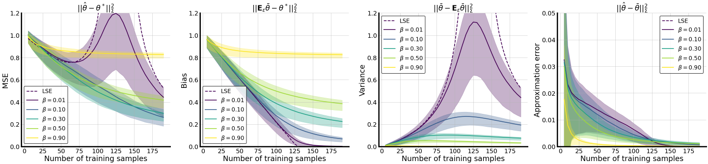
Figure 1: Decomposition of MSE into the bias, variance, and approximation error as in Theorem 4. Our MSE bound is an extension of the traditional bias-variance decomposition by modifying the bias and variance terms to correspond to an estimator with a deterministic regularizer and adding an additional approximation error term to compensate for the error. In this figure, we show that for random mask augmentation with different dropout probability $\beta$, the approximation error is small compared to the bias and variance (being at most $1/10$ of each of these quantities in this case), validating the efficacy of our proposed decomposition.

That the approximation error is negligible is an apriori surprising observation in the high-dimensional regime, as the sample data augmentation covariance $\mathrm{{Cov}}_{\mathcal{G}}(\mathbf{X})$ and its expectation $\mathbb{E}_{\mathbf{x}}[\text{Cov}_{g}(\mathbf{x})]$ are $p$-dimensional square matrices and $p\gg n$. We critically use the special structure of the augmentations we study to show that despite this high-dimensional structure, it is common for $\mathrm{{Cov}}_{\mathcal{G}}(\mathbf{X})$ to converge to its expectation at a rate that depends mostly on $n$ and minimally on $p$.

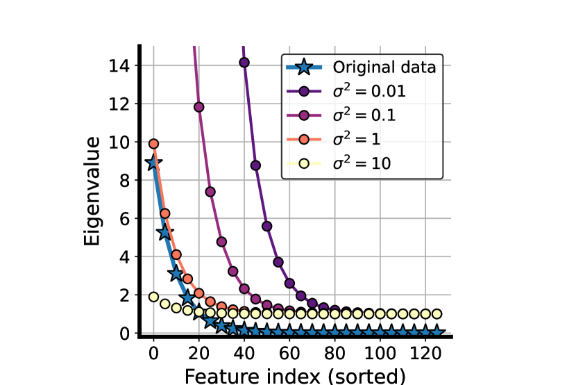
((a)) Noise injection (ridge)

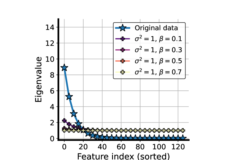
((b)) Pepper noise

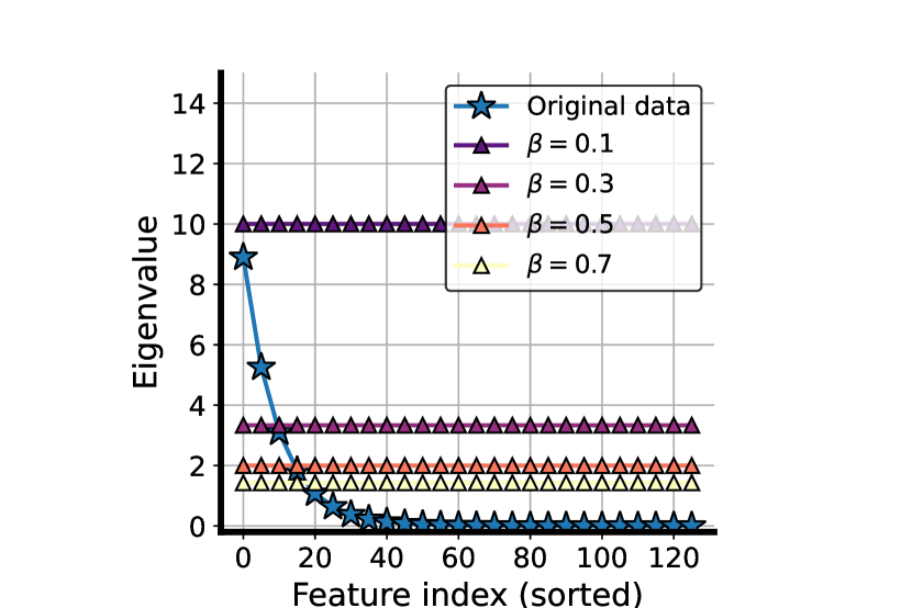
((c)) Random mask

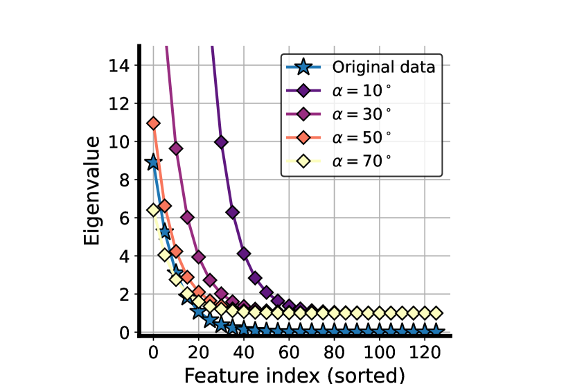
((d)) Random rotation

((e)) Generalization of different augmentations. In this plot, we visualize the bias (x-axis), variance (y-axis), and total MSE (color) for different augmentation and intensity in a regression task. The background color indicates the generalization error. Lighter colors indicate better performance.

Figure 2: Equivalent augmented data spectrum and generalization In plots (a)-(d), we visualize the regularized augmented spectrum (defined in (14))) of Gaussian noise injection (N), pepper noise injection (P), random mask (M) and the novel random rotation (R) introduced in Section 5.2.3, and their corresponding generalization in plot (e), where the number followed by the abbreviation in the data point denotes its parameter. The LSE represents the baseline of least-squared estimator without any augmentation.

To show that our deterministic approximation is validated, i.e., the approximation error term is negligible, we require the following technical assumption, which shows that a normalized version of the empirical augmentation-induced covariance matrix converges as $n,p\to\infty$.

Assumption 1.

Let the data dimension $p$ grows with $n$ at the polynomial rate $p=n^{\alpha}$ for some $\alpha>1$. Then, we assume that for any sequence of data covariance matrices $\{{\boldsymbol{\Sigma}}_{p}\}_{p\geq 1}$, the normalized empirical covariance induced by the augmentation distribution converges to its expectation as $n\to\infty$. More formally, we assume that

$$\Delta_{G}:=\left\|\frac{1}{n}\mathbb{E}_{\mathbf{x}}[\mathrm{{Cov}}_{\mathcal{G}}(\mathbf{x})]^{-\frac{1}{2}}\sum_{i=1}^{n}\mathrm{{Cov}}_{\mathcal{G}}(\mathbf{x}_{i})\mathbb{E}_{\mathbf{x}}[\mathrm{{Cov}}_{\mathcal{G}}(\mathbf{x})]^{-\frac{1}{2}}-\mathbf{I}_{p}\right\|\to 0\text{ as }n\to\infty\text{ almost surely. }$$

We note here that the above should be interpreted as the limit as both $n$ and $p$ grow together. For our subsequent results to be meaningful, it is further required that this convergence is sufficiently fast as $n,p\to\infty$. We will show (in Proposition 5, and with several concrete examples) that a wide class of augmentations will satisfy this assumption and converge at the rate $\mathcal{O}\left(\sqrt{\frac{\log n}{n}}\right)$. We will see that this rate is sufficient for our results to be tight in non-trivial regimes.

4.3 Regression analysis

With the connection of DA to ridge regression established in Section 3.2 and the deterministic approximation method established in Section 4.2, we are ready to present our meta-theorem for the regression setting. The results for the augmented estimators which are unbiased-in-average are presented in Section 4.3.1, and biased-in-average augmented estimators are studied in Section 4.3.2. The applications of the general theorem in this section will be discussed in detail in Section 5.

4.3.1 Regression analysis for general classes of unbiased augmentations

In this section, we present the meta-theorem for estimators induced by unbiased-on-average augmentations (i.e., for which $\mu_{\mathcal{G}}(\mathbf{x})=\mathbf{x}$) in Theorem 4. All proofs in this section can be found in Appendix B. To state the main result of this section, we introduce new notation for the relevant augmentation-transformed quantities.

Definition 3 (Augmentation-transformed quantities).

We define two spectral augmentation transformed quantities, the covariance-of-the-mean-augmentation $\bar{{\boldsymbol{\Sigma}}}$, and augmentation-transformed data covariance ${{\boldsymbol{\Sigma}}}_{aug}$, by

$$\bar{{\boldsymbol{\Sigma}}}:=\mathbb{E}_{\mathbf{x}}[(\mu_{\mathcal{G}}(\mathbf{x})-\mathbb{E}_{\mathbf{x}}[\mu_{\mathcal{G}}(\mathbf{x})])(\mu_{\mathcal{G}}(\mathbf{x})-\mathbb{E}_{\mathbf{x}}[\mu_{\mathcal{G}}(\mathbf{x})])^{\top}],$$ (13)

$${{\boldsymbol{\Sigma}}}_{aug}:=\mathbb{E}_{\mathbf{x}}[\mathrm{{Cov}}_{\mathcal{G}}(\mathbf{x})]^{-1/2}\bar{{\boldsymbol{\Sigma}}}\mathbb{E}_{\mathbf{x}}[\mathrm{{Cov}}_{\mathcal{G}}(\mathbf{x})]^{-1/2},$$ (14)

We also denote the eigenvalues of ${\boldsymbol{\Sigma}}_{aug}$ by $\lambda_{1}^{aug}\geq\lambda_{2}^{aug}\geq\dots\geq\lambda_{p}^{aug}$. Similarly, we define the augmentation-transformed data matrix $\mathbf{X}_{aug}$, and augmentation-transformed model parameter ${\boldsymbol{\theta}}_{aug}^{*}$ as

$$\mathbf{X}_{aug}:=\mu_{G}(\mathbf{X})\mathbb{E}_{\mathbf{x}}[\mathrm{{Cov}}_{\mathcal{G}}(\mathbf{x})]^{-1/2},\leavevmode\nobreak\ {\boldsymbol{\theta}}_{aug}^{*}:=\mathbb{E}_{\mathbf{x}}[\mathrm{{Cov}}_{\mathcal{G}}(\mathbf{x})]^{1/2}\boldsymbol{\theta}^{*}.$$ (15)

Note that since the rows of $\mathbf{X}_{aug}$ are still i.i.d., $\mathbf{X}_{aug}$ can be viewed as a modified data matrix with covariance ${\boldsymbol{\Sigma}}_{aug}$ and $\bar{{\boldsymbol{\Sigma}}}={\boldsymbol{\Sigma}}$ if the augmentation is unbiased in average.

Armed with this notation, we are ready to state our meta-theorem.

Theorem 4 (High probability bound of MSE for unbiased DA).

Consider an unbiased data augmentation $g$ and its corresponding estimator $\hat{\boldsymbol{\theta}}_{\text{aug}}$. Recall the definition

$${\Delta}_{G}:=\|\mathbb{E}_{\mathbf{x}}[\mathrm{{Cov}}_{\mathcal{G}}(\mathbf{x})]^{-\frac{1}{2}}\mathrm{{Cov}}_{\mathcal{G}}(\mathbf{X})\mathbb{E}_{\mathbf{x}}[\mathrm{{Cov}}_{\mathcal{G}}(\mathbf{x})]^{-\frac{1}{2}}-\mathbf{I}_{p}\|,$$

and let $\kappa$ be the condition number of ${\boldsymbol{\Sigma}}_{\text{aug}}$. Assume that the condition numbers for the matrices $\mathcal{A}_{k_{1}}(\mathbf{\mathbf{X}_{\text{aug}}};n)$, $\mathcal{A}_{k_{2}}(\mathbf{\mathbf{X}_{\text{aug}}};n)$ are bounded by $L_{1}$ and $L_{2}$ respectively with probability $1-\delta^{\prime}$, and that ${\Delta}_{G}\leq c^{\prime}$ for some constant $c^{\prime}<1$. Then there exist some constants $c,\leavevmode\nobreak\ C$ depending only on $\sigma_{x}$ and $\sigma_{\varepsilon}$, such that, with probability $1-\delta^{\prime}-4n^{-1}$, the test mean-squared error is bounded by

$$\mathrm{MSE}\leavevmode\nobreak\ \lesssim \leavevmode\nobreak\ {{\color[rgb]{0,0,1}\mathrm{Bias}}+{\color[rgb]{1,0,0}\mathrm{Variance}}+\color[rgb]{0.5,0.5,0}\mathrm{ApproximationError}},$$ (16)

$$\frac{{\color[rgb]{0,0,1}\mathrm{Bias}}}{C_{x}L_{1}^{4}}\leavevmode\nobreak\ \lesssim \leavevmode\nobreak\ {{\left(\left\|\mathbf{P}^{{\boldsymbol{\Sigma}}_{\text{aug}}}_{k_{1}+1:p}{\theta}_{\text{aug}}^{*}\right\|_{{\boldsymbol{\Sigma}}_{\text{aug}}}^{2}+\left\|\mathbf{P}^{{\boldsymbol{\Sigma}}_{\text{aug}}}_{1:k_{1}}{\theta}_{\text{aug}}^{*}\right\|_{{\boldsymbol{\Sigma}}_{\text{aug}}^{-1}}^{2}\frac{(\rho^{\text{aug}}_{k_{1}})^{2}}{{(\lambda^{\text{aug}}_{k_{1}+1})^{-2}}+(\lambda^{\text{aug}}_{1})^{-2}(\rho^{\text{aug}}_{k_{1}})^{2}}\right)}},$$

$$\frac{{\color[rgb]{1,0,0}\mathrm{Variance}}}{\sigma_{\varepsilon}^{2}L_{2}^{2}\tilde{C}_{x}}\leavevmode\nobreak\ \lesssim \leavevmode\nobreak\ {{\left(\frac{k_{2}}{n}+\frac{n}{R^{\text{aug}}_{k}}\right)\log n}},\leavevmode\nobreak\ \leavevmode\nobreak\ {{\color[rgb]{0.5,0.5,0}\mathrm{Approx.Error}}}\leavevmode\nobreak\ \lesssim\leavevmode\nobreak\ \kappa^{\frac{1}{2}}{\Delta}_{G}\left(\|\boldsymbol{\theta}^{*}\|_{{\boldsymbol{\Sigma}}}+\sqrt{\mathrm{Bias}+\mathrm{Variance}}\right).$$

Above, we defined $\rho^{\text{aug}}_{k}:=\rho_{k}({\boldsymbol{\Sigma}}_{\text{aug}};n)$ and $R^{\text{aug}}_{k}:=R_{k}({\boldsymbol{\Sigma}}_{\text{aug}};n)$ as shorthand.

Theorem 4 illustrates the critical role that the spectrum of the augmentation-transformed data covariance ${\boldsymbol{\Sigma}}_{\text{aug}}$ plays in generalization. In Fig. 2, we visualize this impact for various types of augmentations.

When is our bound in Theorem 4 tight?

A natural question is when and whether our bound in Theorem 4 is tight. The tightness of the testing error for an estimator with a fixed regularizer is established (under some additional assumptions on the data distribution, such as sub-Gaussianity and constant condition number) in Theorem 5 of Tsigler and Bartlett (2020). Hence, as long as the approximation error in our theorem is dominated by either the bias or variance, then our bound will also be tight. Roughly speaking this happens when the convergence of $n^{-1}\mathrm{{Cov}}_{\mathcal{G}}(\mathbf{X})$ to $\mathbb{E}_{\mathbf{x}}[\mathrm{{Cov}}_{\mathcal{G}}(\mathbf{x})]$ is sufficiently fast with respect to $n$. For interested readers, we have included the full technical condition in Lemma 35 of Appendix A.

An important class of DA in practice involves independently augmenting each of the features. This class subsumes many prevailing augmentations like random mask, salt-and-pepper, and Gaussian noise injection. Because the augmentation covariance $\text{Cov}_{\mathcal{G}}(\mathbf{x})$ is diagonal for such augmentations, we can simplify Theorem 4, as shown in the next proposition. The proposition shows that this class of augmentation has a reordering effect on the magnitude (or importance) of each feature.

Proposition 5 (Independent Feature Augmentations).

Let $g$ be an independent feature augmentation, and $\pi:\{1,2,\dots,p\}\rightarrow\{1,2,\dots,p\}$ be the function that maps the original feature index to the sorted index according to the eigenvalues of ${{\boldsymbol{\Sigma}}}_{\text{aug}}$ in a non-increasing order. Then, data augmentation has a spectrum reordering effect which changes the MSE through the bias modification:

$$\frac{\text{Bias}}{C_{x}L_{1}^{4}} \lesssim\left\|{\theta}^{*}_{\pi(k_{1}+1:p)}\right\|_{{\Sigma}_{\pi(k_{1}+1:p)}}^{2}+\left\|{\theta}_{\pi(1:k_{1})}^{*}\right\|_{\mathbb{E}_{\mathbf{x}}[\mathrm{{Cov}}_{\mathcal{G}}(\mathbf{x})]^{2}{\Sigma}_{\pi(1:k_{1})}^{-1}}^{2}\frac{(\rho_{k_{1}}^{\text{aug}})^{2}}{{(\lambda^{\text{aug}}_{k_{1}+1})^{-2}}+(\lambda^{\text{aug}}_{1})^{-2}(\rho_{k_{1}}^{\text{aug}})^{2}},$$

where $\pi(a:b)$ denotes the indices of $\pi(a),\pi(a+1),\dots,\pi(b)$. Furthermore, if the variance of each feature augmentation $\operatorname{Var}_{g_{i}}(g_{i}(x))$ is a sub-exponential random variable with sub-exponential norm $\sigma_{i}^{2}$ and mean $\bar{\sigma}_{i}^{2}$, $\forall i\in\{1,2,\dots,p\}$, and $p=O(n^{\alpha})$ for some $\alpha>0$, then there exists a constant $c$, depending only on $\alpha$, such that with probability $1-n^{-1}$,

$${\Delta}_{G}\lesssim\max_{i}\left(\frac{\sigma_{i}^{2}}{\bar{\sigma}_{i}^{2}}\right)\sqrt{\frac{\log n}{n}}.$$

Proposition 5 gives a bound on the approximation error for independent feature augmentations and finds that ${\Delta}_{G}\lesssim\sqrt{\frac{\log n}{n}}$. However, one might wonder whether the approximation error still vanishes for stochastic augmentations that include dependencies between features. While we do not provide such a guarantee for arbitrary augmentations, we present a general technique that we later use to show that the approximation error is indeed vanishing for many popularly used augmentations that include dependencies between features. Specifically, we consider the decomposition $\mathrm{{Cov}}_{\mathcal{G}}(\mathbf{X})=\mathbf{D}+\mathbf{Q}$, where $\mathbf{D}$ is a diagonal matrix representing the independent feature augmentation part. Then, we have

$${\Delta}_{G}\lesssim\frac{\|\mathbf{D}-\mathbb{E}\mathbf{D}\|+\|\mathbf{Q}-\mathbb{E}\mathbf{Q}\|}{\mu_{p}(\mathbb{E}_{\mathbf{x}}\mathrm{{Cov}}_{\mathcal{G}}(\mathbf{x}))}.$$ (17)

Further discussion on the approximation error for dependent feature augmentation, along with the proof of Eq. (17), is provided in Appendix F. We use Eq. (17) to show that the possibly large error of the non-diagonal part $\|\mathbf{Q}-\mathbb{E}\mathbf{Q}\|$ resulting from a dependent feature augmentation can be mitigated by the denominator $\mu_{p}(\mathbb{E}_{\mathbf{x}}\mathrm{{Cov}}_{\mathcal{G}}(\mathbf{x}))$, for augmentations for which $\mathbb{E}_{\mathbf{x}}\mathrm{{Cov}}_{\mathcal{G}}(\mathbf{x})$ is well-conditioned. We use this in Appendix F to characterize the approximation error for two examples of augmentations that induce dependencies between features: a) the new random-rotation augmentation that we introduced in Section 3.4, b) the cutout augmentation which is popular in deep learning practice (DeVries and Taylor, 2017).

4.3.2 Regression analysis for general biased on average augmentations

All of our analysis thus far has assumed that the augmentation is unbiased on average, i.e. that $\mu_{\mathcal{G}}(\mathbf{x})=\mathbf{x}$. We now derive and interpret the expression for the estimator that is induced by a general augmentation that can be biased. We introduce the following additional definitions.

Definition 6.

We define the augmentation bias and bias covariance induced by the augmentation $g$ as

$$\xi(\mathbf{x}):=\mu_{g}(\mathbf{x})-\mathbf{x},\leavevmode\nobreak\ \leavevmode\nobreak\ \operatorname{Cov}_{\xi}:=\mathbb{E}_{\mathbf{x}}\left[\xi(\mathbf{x})\xi(\mathbf{x})^{\top}\right].$$ (18)

Since $\xi(\mathbf{x})$ is not zero for a biased augmentation, the expression in (7) becomes more complicated and we lose the exact equivalence to an ridge regression in (3.2)). This is because biased DA induces a distribution-shift in the training data that does not appear in the test data. Our next result for biased estimators, which is strictly more general than Theorem 4, will show that this distribution-shift affects the test MSE through both covariate-shift as well as label-shift. To facilitate analysis, we impose the natural assumption that the mean augmentation $\mu(\mathbf{x})$ remains sub-Gaussian.

Assumption 2.

For the input data $\mathbf{x}$, the mean transformation $\mu(\mathbf{x})$ admits the form $\mu(\mathbf{x})=\bar{{\boldsymbol{\Sigma}}}^{1/2}\bar{\mathbf{z}}$, where $\bar{{\boldsymbol{\Sigma}}}$ is defined in Definition 3 and $\bar{\mathbf{z}}$ is a centered and isotropic sub-Gaussian vector with sub-Gaussian norm $\sigma_{\bar{z}}$.

We also recall the definition of the mean augmentation covariance $\bar{{\boldsymbol{\Sigma}}}:=\mathbb{E}_{\mathbf{x}}[(\mu_{\mathcal{G}}(\mathbf{x})-\mathbb{E}_{\mathbf{x}}[\mu_{\mathcal{G}}(\mathbf{x})])(\mu_{\mathcal{G}}(\mathbf{x})-\mathbb{E}_{\mathbf{x}}[\mu_{\mathcal{G}}(\mathbf{x})])^{\top}]$. Now we are ready to state our theorem for biased augmentations. The proof is deferred to Appendix B.3.

Theorem 7 (Bounds on the MSE for Biased Augmentations).

Consider the estimator $\hat{\boldsymbol{\theta}}_{\text{aug}}$ obtained by solving the aERM in (2). Let $\mathrm{MSE}^{o}(\hat{\boldsymbol{\theta}}_{\text{aug}})$ denote the unbiased MSE bound in Eq. (16) of Theorem 4, and recall the definition

$$\Delta_{G}:=\left\|\frac{1}{n}\mathbb{E}_{\mathbf{x}}[\mathrm{{Cov}}_{\mathcal{G}}(\mathbf{x})]^{-\frac{1}{2}}\sum_{i=1}^{n}\mathrm{{Cov}}_{\mathcal{G}}(\mathbf{x}_{i})\mathbb{E}_{\mathbf{x}}[\mathrm{{Cov}}_{\mathcal{G}}(\mathbf{x})]^{-\frac{1}{2}}-\mathbf{I}_{p}\right\|.$$

Suppose the assumptions in Theorem 4 hold for the mean augmentation $\mu(\mathbf{x})$ and that ${\Delta}_{G}\leq c<1$. Then with probability $1-\delta^{\prime}-4n^{-1}$ we have,

$$\leavevmode\nobreak\ \mathrm{MSE}(\hat{\boldsymbol{\theta}}_{\text{aug}})\lesssim R_{1}^{2}\cdot\left(\sqrt{\mathrm{MSE}^{o}(\hat{\boldsymbol{\theta}}_{\text{aug}})}+R_{2}\right)^{2},$$

where

$$R_{1} =1+\|{\boldsymbol{\Sigma}}^{\frac{1}{2}}\bar{{\boldsymbol{\Sigma}}}^{-\frac{1}{2}}-\mathbf{I}_{p}\|\text{ and }$$

$$R_{2} =\sqrt{{\|\bar{{\boldsymbol{\Sigma}}}(\mathbb{E}_{\mathbf{x}}[\mathrm{{Cov}}_{\mathcal{G}}(\mathbf{x})])^{-1}\|}}\left(1+\frac{{\Delta}_{G}}{1-c}\right)\left(\sqrt{{\Delta}_{\xi}}\|\boldsymbol{\theta}^{*}\|+\|\boldsymbol{\theta}^{*}\|_{\operatorname{Cov}_{\xi}}\right)$$

$$\times\left(\sqrt{\frac{1}{\lambda_{k}^{\text{aug}}}}+\sqrt{\frac{\lambda_{k+1}^{\text{aug}}(1+\rho_{k}^{aug})}{(\lambda_{1}^{\text{aug}}\rho_{0}^{aug})^{2}}}\right).$$

Our upper bound for the MSE in the biased augmentation case is a generalization of the bound in Tsigler and Bartlett (2020) to the scenario with distribution-shift. This result shows that two different factors can cause generalization error over and above the unbiased case: 1. covariate shift, which is reflected in the multiplicative factor $R_{1}$; this term occurs because we are testing the estimator on a distribution with covariance ${\boldsymbol{\Sigma}}$ but our training covariates have covariance $\bar{{\boldsymbol{\Sigma}}}$ instead, 2. label shift, which manifests itself as the additive error given by $R_{2}$. This term arises from the training mismatch between the true covariate observation and mean augmented covariate (i.e., $\mathbf{X}$ v.s. $\mu_{G}(\mathbf{X})$). As a sanity check, we can see that $R_{1}=1$ and $R_{2}=0$ when the augmentation is unbiased in average, i.e., $\mu_{\mathcal{G}}(\mathbf{x})=\mathbf{x},\leavevmode\nobreak\ \forall\mathbf{x}$, since ${\boldsymbol{\Sigma}}=\bar{{\boldsymbol{\Sigma}}}$, $\Delta_{\delta}=0$ and $\operatorname{Cov}_{\delta}=0$. Thus, we directly recover Theorem 4 in this case. Whether Theorem 7 is tight in general is an interesting open question for future work.

4.4 Classification analysis

In this subsection, we state the meta-theorem for generalization of DA in the classification task. We follow a similar path for the analysis as in regression by appealing to the connection between DA and ridge estimators and the deterministic approximation strategy outlined above. While the results in this section operate under stronger assumptions, we provide a similar set of results to the regression case. The primary aim of these results is to compare the generalization behavior of DA between regression and classification settings, which we do in depth in Section 5.

4.4.1 Classification analysis setup

We adopt the random signed model from Muthukumar et al. (2021), noting that we expect similar analysis to be possible for the Gaussian-mixture-model setting of Chatterji and Long (2021); Wang and Thrampoulidis (2021) (we defer such analysis to a companion paper). Given a target vector $\theta^{*}\in\mathbb{R}^{d}$ and a label noise parameter $0\leq\nu^{*}<1/2$, we assume the data are generated as binary labels $y_{i}\in\{-1,1\}$ according to the signal model

$$y_{i}=\begin{cases}\operatorname{sgn}(\mathbf{x}_{i}^{\top}\boldsymbol{\theta}^{*})\quad&\text{with probability}\,1-\nu^{*}\\ -\operatorname{sgn}(\mathbf{x}_{i}^{\top}\boldsymbol{\theta}^{*})\quad&\text{with probability}\,\nu^{*}\\ \end{cases}$$ (19)

Just as in Muthukumar et al. (2021), we make a 1-sparse assumption on the true signal $\boldsymbol{\theta}^{*}=\frac{1}{\sqrt{\lambda_{t}}}\mathbf{e}_{t}$. We denote $\mathbf{x}_{\text{sig}}:=\mathbf{x}_{t}$ to emphasize the signal feature. Motivated by recent results which demonstrate the effectiveness of training with the squared loss for classification tasks (Hui and Belkin, 2020; Muthukumar et al., 2021), we study the classification risk of the estimator $\hat{\boldsymbol{\theta}}$ which is computed by solving the aERM objective on the binary labels $y_{i}$ with respect to the squared loss (Eq. (2)).

Muthukumar et al. (2021) showed that two quantities, survival and contamination, play key roles in characterizing the risk, akin to the bias and variance in the regression task (in fact, as shown in the proof of Lemma 39, the contamination term scales identically to the variance from regression analysis). The definitions of these quantities are given below.

Definition 8 (Survival and contamination (Muthukumar et al., 2021)).

Given an estimator $\hat{\theta}$, its survival (SU) and contamination (CN) are defined as

$$\mathrm{SU(\hat{\boldsymbol{\theta}})}=\sqrt{\lambda_{t}}\hat{\boldsymbol{\theta}}_{t},\leavevmode\nobreak\ \leavevmode\nobreak\ \mathrm{CN(\hat{\boldsymbol{\theta}})}=\sqrt{\sum_{j=1,j\neq t}^{p}\lambda_{j}\hat{\boldsymbol{\theta}}_{j}^{2}}.$$ (20)

For Gaussian data, Muthukumar et al. (2021) derived the following closed-form expression for the POE:

$$\text{POE}(\hat{\boldsymbol{\theta}})=\frac{1}{2}-\frac{1}{\pi}\tan^{-1}\frac{\mathrm{SU(\hat{\boldsymbol{\theta}})}}{\mathrm{CN(\hat{\boldsymbol{\theta}})}}.$$ (21)

Thus, the POE depends on the ratio between survival SU and contamination CN, essentially a kind of signal-to-noise ratio for the classification task. In this work, we prove that a similar principle arises when we consider training with data augmentation in more general correlated input distributions. Formally, we make the following assumption on the true signal and input distribution for our classification analysis.

Assumption 3.

Assume the target signal is 1-sparse and given by $\boldsymbol{\theta}^{*}=\frac{1}{\sqrt{\lambda_{t}}}\mathbf{e}_{t}$. Additionally, assume the input can be factored as $\mathbf{x}={\boldsymbol{\Sigma}}^{\frac{1}{2}}\mathbf{z}$, where ${\boldsymbol{\Sigma}}\succeq 0$ is diagonal, and $\mathbf{z}$ is a sub-Gaussian random vector with norm $\sigma_{z}$ and uniformly bounded density. We denote $\mathbf{x}_{\text{sig}}=\mathbf{x}_{t}$ and $\mathbf{x}_{\text{noise}}=[\mathbf{x}_{1},\dots,\mathbf{x}_{t-1},\mathbf{x}_{t+1},\dots,\mathbf{x}_{p}]^{T}$. We further assume that the signal and noise features are independent, i.e., $\mathbf{x}_{\text{sig}}\perp\mathbf{x}_{\text{noise}}$.

Similar to the regression case, our classification analysis consists of 1) expressing the excess risk in terms of $\bar{\boldsymbol{\theta}}_{\text{aug}}$, the estimator corresponding to the averaged augmented covariance $\mathbb{E}_{\mathbf{x}}[\text{Cov}_{g}(\mathbf{x})]$, 2) arguing that the survival and contamination can be viewed as the equivalent quantities for a ridge estimator with a modified data spectrum, and 3) upper and lower bounding the survival and contamination of this ridge estimator. As in the case of regression analysis, step 1) is the most technically involved.

4.4.2 Classification analysis for unbiased augmentations

Now, we present our main theorem for the classification task. The proof of this theorem is deferred to Appendix C.

Theorem 9 (Bounds on Probability of Classification Error).

Consider the classification task under the setting in Assumption 3. Recall that $\hat{\boldsymbol{\theta}}_{\text{aug}}$ is the estimator solving the aERM objective in (2) and the definition ${\Delta}_{G}:=\|\text{Cov}_{G}(\mathbf{X})-\mathbb{E}_{\mathbf{x}}[\text{Cov}_{g}(\mathbf{x})]\|$. Let $t\leq n$ be the index (arranged according to the eigenvalues of ${{\boldsymbol{\Sigma}}}_{\text{aug}}$) of the non-zero coordinate of the true signal, $\widetilde{{\boldsymbol{\Sigma}}}_{\text{aug}}$ be the leave-one-out modified spectrum corresponding to index $t$, $\kappa$ be the condition number of ${\boldsymbol{\Sigma}}_{\text{aug}}$, and $\widetilde{\mathbf{X}}_{\text{aug}}$ be the leave-one-column-out data matrix corresponding to column $t$.

Suppose data augmentation is performed independently for $\mathbf{x}_{sig}$ and $\mathbf{x}_{noise}$, and there exists a $t\leq k\leq n$ such that with probability at least $1-\delta$, the condition numbers of $n\mathbf{I}+\widetilde{\mathbf{X}}^{\text{aug}}_{k+1:p}(\mathbf{X}^{\text{aug}}_{k+1:p})^{\top}$ and $n\mathbf{I}+{\mathbf{X}}^{\text{aug}}_{k+1:p}(\mathbf{X}^{\text{aug}}_{k+1:p})^{\top}$ are at most $L$, and that of $\widetilde{\mathbf{X}}_{k+1:p}{\boldsymbol{\Sigma}}_{k+1:p}\widetilde{\mathbf{X}}_{k+1:p}^{T}$ is at most $L_{1}$. Then as long as $\|\bar{\boldsymbol{\theta}}_{\text{aug}}-\hat{\boldsymbol{\theta}}_{\text{aug}}\|_{{\boldsymbol{\Sigma}}}=O(\mathrm{SU})$ and $\|\bar{\boldsymbol{\theta}}_{\text{aug}}-\hat{\boldsymbol{\theta}}_{\text{aug}}\|_{{\boldsymbol{\Sigma}}}=O(\mathrm{CN})$, with probability $1-\delta-\exp(-\sqrt{n})-5n^{-1}$, the probability of classification error (POE) can be bounded in terms of the survival ($\mathrm{SU}$) and contamination ($\mathrm{CN}$), as

$$\mathrm{POE}(\hat{\theta})\leavevmode\nobreak\ \lesssim\leavevmode\nobreak\ \frac{{\color[rgb]{1,0,0}\mathrm{CN}}}{\mathrm{{\color[rgb]{0,0,1}SU}}}\left(1+\sigma_{z}\sqrt{\log{\frac{{\color[rgb]{0,0,1}\mathrm{SU}}}{\mathrm{{\color[rgb]{1,0,0}CN}}}}}\right),$$ (22)

where

$$\frac{\lambda^{\text{aug}}_{t}(1-2\nu^{*})\left(1-\frac{k}{n}\right)}{L\left(\lambda^{\text{aug}}_{k+1}\rho_{k}({\boldsymbol{\Sigma}}_{\text{aug}};n)+\lambda_{t}^{\text{aug}}L\right)}\leavevmode\nobreak\ \lesssim\leavevmode\nobreak\ \underbrace{{\color[rgb]{0,0,1}\mathrm{SU}}}_{\text{Survival}}\leavevmode\nobreak\ \lesssim\leavevmode\nobreak\ \frac{L\lambda^{\text{aug}}_{t}(1-2\nu^{*})}{\lambda^{\text{aug}}_{k+1}\rho_{k}({\boldsymbol{\Sigma}}_{\text{aug}};n)+L^{-1}\lambda^{\text{aug}}_{t}\left(1-\frac{k}{n}\right)},$$ (23)

$$\sqrt{\frac{\tilde{\lambda}_{k+1}^{aug}\rho_{k}(\tilde{{\boldsymbol{\Sigma}}}_{aug}^{2};0)}{L^{\prime 2}(\lambda_{1}^{aug})^{2}(1+\rho_{0}({\boldsymbol{\Sigma}}_{aug};\lambda))^{2}}}\leavevmode\nobreak\ \lesssim\underbrace{{\color[rgb]{1,0,0}\mathrm{CN}}}_{\text{Contamination}} \lesssim\leavevmode\nobreak\ \sqrt{(1+\mathrm{SU}^{2})L^{2}\left(\frac{k}{n}+\frac{n}{R_{k}(\tilde{{\boldsymbol{\Sigma}}}_{\text{aug}};n)}\right)\log n}$$ (24)

Furthermore, if $\mathbf{x}$ is Gaussian, then we obtain even tighter bounds:

$$\frac{1}{2}-\frac{1}{\pi}\tan^{-1}c\frac{{\color[rgb]{0,0,1}\mathrm{SU}}}{{\color[rgb]{1,0,0}\mathrm{CN}}}\leavevmode\nobreak\ \leq\leavevmode\nobreak\ \mathrm{POE}(\hat{\boldsymbol{\theta}}_{\text{aug}})\leavevmode\nobreak\ \leq\leavevmode\nobreak\ \frac{1}{2}-\frac{1}{\pi}\tan^{-1}\frac{1}{c}\frac{{\color[rgb]{0,0,1}\mathrm{SU}}}{{\color[rgb]{1,0,0}\mathrm{CN}}}\leavevmode\nobreak\ \lesssim\leavevmode\nobreak\ {\frac{{\color[rgb]{1,0,0}\mathrm{CN}}}{{\color[rgb]{0,0,1}\mathrm{SU}}}},$$ (25)

where $c$ is a universal constant.

Remark 10.

Based on the expression for the classification error for Gaussian data, we see that the survival needs to be asymptotically greater than the contamination for the POE to approach $0$ in the limit as $n,p\to\infty$. We note that the general upper bound we provide matches the tight upper and lower bounds for the Gaussian case up a log factor. Furthermore, the condition $\|\bar{\boldsymbol{\theta}}_{\text{aug}}-\hat{\boldsymbol{\theta}}_{\text{aug}}\|_{{\boldsymbol{\Sigma}}}=O(\mathrm{SU})$ and $\|\bar{\boldsymbol{\theta}}_{\text{aug}}-\hat{\boldsymbol{\theta}}_{\text{aug}}\|_{{\boldsymbol{\Sigma}}}=O(\mathrm{CN})$ is related to our condition for the tightness of our regression analysis, but a bit stronger (because our regression analysis only requires one of these relations to be true). We characterize when this stronger condition is met in Lemma 42.

Based on the upper and lower bounds provided for SU and CN, we see that these quantities depend crucially on the spectral properties of the induced covariance matrix ${\boldsymbol{\Sigma}}_{aug}$. For favorable classification performance, Theorem 9 also requires $t\leq n$. This is a necessary product of our analogy to a ridge estimator and is equivalent to requiring that $\theta_{\text{aug}}^{*}$ lies within the eigenspace corresponding to the dominant eigenvalues of the spectrum ${\boldsymbol{\Sigma}}_{aug}$. Such requirements have also been used in past analyses of both regression (Tsigler and Bartlett, 2020) and classification (Muthukumar et al., 2021).

4.4.3 Classification analysis for general biased augmentations

As a counterpart of our regression analysis for estimators induced by biased-on-average augmentations (i.e. $\mu_{g}(\mathbf{x})\neq\mathbf{x}$), we would also like to understand the impact of augmentation-induced bias on classification. Interestingly, the effect of this bias in classification turns out to be much more benign than that in regression. As a simple example, consider a scaling augmentation of the type $g(\mathbf{x}):=2\mathbf{x}$. The induced bias is $\mu_{g}(\mathbf{x})-\mathbf{x}=\mathbf{x}$, and the trained estimator $\hat{\boldsymbol{\theta}}_{\text{aug}}$ is just half the estimator trained with $\mathbf{x}$, which, however, predicts the same labels in a classification task. Therefore, we conclude that even with a large bias, the resultant estimator might be equivalent to the original one for classification tasks. In fact, as we show in the next result, augmentation bias is benign for the classification error metric under relatively mild conditions. The proof of this result is provided in Appendix Theorem 11.

Theorem 11 (POE of biased estimators).

Consider the 1-sparse model $\boldsymbol{\theta}^{*}=\mathbf{e}_{t}$. and let $\hat{\boldsymbol{\theta}}_{\text{aug}}$ be the estimator that solves the aERM in (2) with biased augmentation (i.e., $\mu(\mathbf{x})\neq\mathbf{x}$). Let Assumption 2 holds, and the assumptions of Theorem 9 be satisfied for data matrix $\mu(\mathbf{X})$. If the mean augmentation $\mu(\mathbf{x})$ modifies the $t$-th feature independently of other features and the sign of the $t$-th feature is preserved under the mean augmentation transformation, i.e., $\operatorname{sgn}\left(\mu(\mathbf{x})_{t}\right)=\operatorname{sgn}\left(\mathbf{x}_{t}\right),$ $\forall\mathbf{x}$, then, the POE($\hat{\boldsymbol{\theta}}_{\text{aug}}$) is upper bounded by

$$\mathrm{POE}(\hat{\boldsymbol{\theta}}_{\text{aug}})\leq\mathrm{POE}^{o}(\hat{\boldsymbol{\theta}}_{\text{aug}}),$$ (26)

where $\mathrm{POE}^{o}(\hat{\boldsymbol{\theta}}_{\text{aug}})$ is any bound in Theorem 9 with $\mathbf{X}$ and ${\boldsymbol{\Sigma}}$ replaced by $\mu(\mathbf{X})$ and $\bar{{\boldsymbol{\Sigma}}}$, respectively.

Note that the sign preservation is only required in expectation and not for every realization of the augmentation, i.e., we only require $\mathbb{E}_{g}\left[g(\mathbf{x})_{t}\right]$ has the same sign as $\mathbf{x}_{t}$, rather than requiring that $g(\mathbf{x})_{t}$ have the same sign as $\mathbf{x}_{t}$ for every realization of $g$. The latter label-preserving property is is much more stringent and has been studied in Wu et al. (2020). At a high level, this result tells us that as long as the signal feature preserves the sign under the mean augmentation, the classification error is purely determined by the modified spectrum induced by DA.

In Fig. 3, we simulate the biased and unbiased random mask augmentation (He et al., 2022) and test their performance in regression and classification tasks. We consider the 1-sparse model in $\mathbb{R}^{128}$ (i.e. $p=128$) with isotropic Gaussian covariates. For the biased variant of random mask, we use the masked estimator without the normalization factor $(1-\beta)$; therefore, the augmentation mean is equal to $\mu_{g}(\mathbf{x})=(1-\beta)\mathbf{x}$. From the figure, we see the bias can be very harmful in regression, especially in the overparametrized regime ($n\leq 128$), while the performance is identical for classification. This experiment demonstrates the sharp differences in behavior between the settings of Theorems 7 and 11. We discuss this observation further in Section 5.3.

5 The good, the bad and the ugly sides of data augmentation

In this section, we will use the meta-theorems established in Section 4.3 and 4.4 to get further insight into the impact of DA on generalization. First, in Section 5.1, we derive generalization bounds for many common augmentations. Then, in Section 5 we use these bounds to understand when DA can be helpful or harmful. Finally, in Section 5.1 we conclude by discussing the complex range of factors (the “ugly”) that play an important role in determining the effect of DA.

5.1 Case studies: generalization of common DA

In this section, we present and interpret generalization guarantees for commonly used augmentations including Gaussian noise injection, randomized mask, cutout, and salt-and-pepper noise. In particular, we discuss whether these augmentations improve or worsen generalization compared to the LSE estimator, beginning with regression tasks.

5.1.1 Gaussian noise injection

As a preliminary example, we note that Proposition 5 generalizes and recovers the existing bounds on the ridge and ridgeless estimators (Bartlett et al., 2020; Tsigler and Bartlett, 2020). This is consistent with classical results (Bishop, 1995) that show an equivalence between augmented ERM with Gaussian noise injection and ridge regularization. For completeness, we include the generalization bounds for Gaussian noise injection in Appendix B.5.

5.1.2 Randomized masking

Next, we consider the popular randomized masking augmentation (both the biased and unbiased variants), in which each coordinate of each data vector is set to $0$ with a given probability, denoted by the masking parameter $\beta\in[0,1]$. The unbiased variant of randomized masking rescales the features so that the augmented features are unbiased in expectation. This type of augmentation has been widely used in practice (He et al., 2022; Konda et al., 2015), and is a simplified version of the popular cutout augmentation (DeVries and Taylor, 2017).

The following corollary characterizes the generalization error arising from the randomized masking augmentation in regression tasks.

Corollary 12 (Regression bounds for unbiased randomized masking augmentation).

Consider the unbiased randomized masking augmentation $g(\mathbf{x})=[b_{1}\mathbf{x}_{1},\dots,b_{p}\mathbf{x}_{p}]/(1-\beta)$, where $b_{i}$ are i.i.d. Bernoulli$(1-\beta)$. Define $\psi=\frac{\beta}{1-\beta}\in[0,\infty)$. Let $L_{1}$, $L_{2}$, $\kappa$, $\delta^{\prime}$ be universal constants as defined in Theorem 4. Assume $p=O(n^{\alpha})$ for some $\alpha>0$. Then, for any set $\mathcal{K}\subset\{1,2,\dots,p\}$ consisting of $k_{1}$ elements and some choice of $k_{2}\in[0,n]$, there exists some constant $c^{\prime}$, which depends solely on $\sigma_{z}$ and $\sigma_{\varepsilon}$ (the sub-Guassian norms of the covariates and noise), such that the regression MSE is upper-bounded by

$$\mathrm{MSE}\lesssim \underbrace{\left\|{\theta}^{*}_{\mathcal{K}}\right\|_{{\Sigma}_{\mathcal{K}}}^{2}+\left\|{\theta}_{\mathcal{K}^{c}}^{*}\right\|_{{\Sigma}_{\mathcal{K}^{c}}}^{2}\frac{(\psi n+p-k_{1})^{2}}{n^{2}+(\psi n+p-k_{1})^{2}}}_{\mathrm{Bias}}$$

$$+ \underbrace{\left(\frac{k_{2}}{n}+\frac{n(p-k_{2})}{(\psi n+p-k_{2})^{2}}\right)\log n}_{\mathrm{Variance}}+\underbrace{\sigma^{2}_{z}\sqrt{\frac{\log n}{n}}\|\boldsymbol{\theta}^{*}\|_{{\boldsymbol{\Sigma}}}}_{\mathrm{Approx.Error}}$$

with probability at least $1-\delta^{\prime}-n^{-1}$.

Noting that $\psi=\frac{\beta}{1-\beta}$ increases monotonically in the mask probability $\beta$, Corollary 12 shows that bias increases with the mask intensity $\beta$, while the variance decreases. Figure 1 empirically illustrates these phenomena through a bias-variance decomposition. In fact, the regression MSE is proportional to the expression for MSE of the least-squares estimator (LSE) on isotropic data, suggesting that randomized masking essentially has the effect of isotropizing the data. As prior work on overparameterized linear models demonstrates (Muthukumar et al., 2020; Hastie et al., 2019; Bartlett et al., 2020), the LSE enjoys particularly low variance, but particularly high bias when applied to isotropic, high-dimensional data. For this reason, random masking turns out to be superior to Gaussian noise injection in reducing variance, but much more inferior in mitigating bias. We explore these effects and compare the overall generalization guarantees of the two types of augmentations in depth in Section 6.2. Our experiments there show striking differences in the manifested effect of these augmentations on generalization, despite their superficial similarities.

We also not here that the approximation error is relatively minimal, of the order $\sqrt{\frac{\log n}{n}}$. It is easily checked that the approximation error is dominated by the bias and variance as long as $p\ll n^{2}$ (and hence the lower bounds of Tsigler and Bartlett (2020) imply tightness of our bound in this range). We next present our generalization guarantees for the biased variant of the random masking augmentation. We verify the behavior predicted by this corollary in Figure 3.

Corollary 13 (Regression bounds for biased mask augmentation).

Consider the biased random mask augmentation $g(\mathbf{x})=[b_{1}\mathbf{x}_{1},\dots,b_{p}\mathbf{x}_{p}]$, where $b_{i}$ are i.i.d. Bernoulli $(1-\beta)$), and carry over all the notation from Corollary 12. Then, the regression MSE is upper bounded by

$${\mathrm{MSE}(\hat{\boldsymbol{\theta}}_{\text{aug}})}\leq\left(\sqrt{\mathrm{MSE}^{o}}+\psi\left(1+\frac{\log n}{n}\right)\cdot\left(\left(\lambda_{1}+\frac{\sum_{j}\lambda_{j}}{n}\right)\|\boldsymbol{\theta}^{*}\|+\|\boldsymbol{\theta}^{*}\|_{{\boldsymbol{\Sigma}}}\right)\right)^{2},$$

with probability at least $1-\delta^{\prime}-n^{-1}$. Above, $\mathrm{MSE}^{o}$ is the RHS of the bound in Corollary 12.

Finally, we characterize the generalization error of the randomized masking augmentation for the classification task.

Corollary 14 (Classification bounds for random mask augmentation).

Let $\hat{\boldsymbol{\theta}}_{\text{aug}}$ be the estimator computed by solving the aERM objective on binary labels with mask probability $\beta$, and denote $\psi:=\frac{\beta}{1-\beta}$. Assume $p\ll n^{2}$. Then, with probability at least $1-\delta-\exp(-\sqrt{n})-5n^{-1}$

$$\mathrm{POE} \lesssim Q^{-1}(1+\sqrt{\log{Q}}),$$ (27)

$$\leavevmode\nobreak\ {\text{where }}Q =\leavevmode\nobreak\ (1-2\nu)\sqrt{\frac{n}{p\log n}}\left(1+\frac{n}{n\psi+p}\right)^{-1}.$$ (28)

In addition, if we assume the input data has Gaussian features, then we have tight generalization bounds

$$\mathrm{POE}\asymp\leavevmode\nobreak\ \frac{1}{2}-\frac{1}{\pi}\tan^{-1}Q$$ (29)

with the same probability.

5.1.3 Random cutout

Next, we consider the popularly used cutout augmentation (DeVries and Taylor, 2017), which picks a set of $k$ (out of $p$) consecutive data coordinates at random and sets them to zero. Interestingly, our analysis shows that the effect of the cutout augmentation is very similar to the simpler-to-analyze random mask augmentation. The following corollary shows that the generalization error of cutout is equivalent to that of randomized masking with dropout probability $\beta=\frac{k}{p}$. The proof of this corollary can be found in Appendix B.5.

Corollary 15 (Generalization of random cutout).

Let $\hat{\boldsymbol{\theta}}^{\text{cutout}}_{k}$ denote the random cutout estimator that zeroes out $k$ consecutive coordinates (the starting location of which is chosen uniformly at random). Also, let $\hat{\boldsymbol{\theta}}^{\text{mask}}_{\beta}$ be the random mask estimator with the masking probability given by $\beta$. We assume that $k=O(\sqrt{\frac{n}{\log p}})$. Then, for the choice $\beta=\frac{k}{p}$ we have

$$\mathrm{MSE}(\hat{\boldsymbol{\theta}}^{\text{cutout}}_{k})\asymp\mathrm{MSE}(\hat{\boldsymbol{\theta}}^{\text{mask}}_{\beta}),\leavevmode\nobreak\ \leavevmode\nobreak\ \mathrm{POE}(\hat{\boldsymbol{\theta}}^{\text{cutout}}_{k})\asymp\mathrm{POE}(\hat{\boldsymbol{\theta}}^{\text{mask}}_{\beta}).$$

This result is consistent with our intuition, as the cutout augmentation zeroes out $\frac{k}{p}$ coordinates on average.

5.1.4 Composite augmentation: Salt-and-pepper

Our meta-theorem can also be applied to compositions of multiple augmentations. As a concrete example, we consider a “salt-and-pepper” style augmentation in which each coordinate is either replaced by random Gaussian noise with a given probability, or otherwise retained. Specifically, salt-and-pepper augmentation modifies the data as $g(\mathbf{x})=[\mathbf{x}^{\prime}_{1},\dots,\mathbf{x}^{\prime}_{p}]$, where $\mathbf{x}^{\prime}_{i}=\mathbf{x}_{i}/(1-\beta)$ with probability $1-\beta$ and otherwise $\mathbf{x}_{i}^{\prime}=\mathcal{N}(\mu,\sigma^{2})/(1-\beta)$. This is clearly a composite augmentation made up of randomized masking and Gaussian noise injection. For simplicity, we only consider the case where $\mu=0$, since it results in an augmentation which is unbiased on average. The regression error of this composite augmentation is described in the following corollary, which is proved in Appendix B.5.

Corollary 16 ( Generalization of Salt-and-Pepper augmentation in regression).

The bias, variance and approximation error of the estimator that are induced by salt-and-pepper augmentation (denoted by $\hat{\boldsymbol{\theta}}_{\text{pepper}}(\beta,\sigma^{2})$) are respectively given by:

$$\mathrm{Bias}[\hat{\boldsymbol{\theta}}_{\text{pepper}}(\beta,\sigma^{2})]\leavevmode\nobreak\ \lesssim\leavevmode\nobreak\ \left(\frac{\lambda_{1}(1-\beta)+\sigma^{2}}{\sigma^{2}}\right)^{2}\mathrm{Bias}\left[\hat{\boldsymbol{\theta}}_{\text{gn}}\left(\frac{\beta\sigma^{2}}{(1-\beta)^{2}}\right)\right],$$

$$\mathrm{Variance}[\hat{\boldsymbol{\theta}}_{\text{pepper}}(\beta,\sigma^{2})]\leavevmode\nobreak\ \lesssim\leavevmode\nobreak\ \mathrm{Variance}\left[\hat{\boldsymbol{\theta}}_{\text{gn}}\left(\frac{\beta\sigma^{2}}{(1-\beta)^{2}}\right)\right],$$

$$\mathrm{Approx.Error}[\hat{\boldsymbol{\theta}}_{\text{pepper}}(\beta,\sigma^{2})]\leavevmode\nobreak\ \asymp\leavevmode\nobreak\ \mathrm{Approx.Error}[\hat{\boldsymbol{\theta}}_{\text{rm}}(\beta)].$$

where $\hat{\boldsymbol{\theta}}_{\text{gn}}(z^{2})$ and $\hat{\boldsymbol{\theta}}_{\text{rm}}(\gamma)$ denotes the estimators that are induced by Gaussian noise injection with variance $z^{2}$ and random mask with dropout probability $\gamma$, respectively. Moreover, the limiting MSE as $\sigma\to 0$ reduces to the MSE of the estimator induced by random masking (denoted by $\hat{\boldsymbol{\theta}}_{\text{rm}}(\beta)$):

$$\lim_{\sigma\rightarrow 0}\mathrm{MSE}[\hat{\boldsymbol{\theta}}_{\text{pepper}}(\beta,\sigma^{2})]=\mathrm{MSE}[\hat{\boldsymbol{\theta}}_{\text{rm}}(\beta)].$$

Corollary 16 clearly indicates that the generalization performance of the salt-and-pepper augmentation interpolates between that of the random mask and Gaussian noise injections, in the sense that it reduces to random mask in the limit of $\sigma\rightarrow 0$, and also has a comparable bias and variance to Gaussian noise injection. More precisely, as we show in the proof of this corollary, this interpolation property is a result of the fact that the eigenvalues of the augmented covariance are the harmonic mean of the eigenvalues induced by random mask and Gaussian noise injection respectively, i.e.

$$\lambda_{{pepper}}(\beta,\sigma^{2})^{-1}=\lambda_{{rm}}(\beta)^{-1}+\beta^{-1}\lambda_{{gn}}(\sigma^{2})^{-1}.$$ (30)

5.2 The good and bad of DA: when is it helpful or harmful?

Armed with generalization guarantees for many common augmentations, we now shift our focus to identifying explicit scenarios in which DA can be helpful or harmful.

5.2.1 The bad: the increase in bias might outweigh the variance reduction

In this section, we consider two different types of common augmentations that suffer from poor generalization in the overparameterized regime. The first is the randomized masking augmentation, whose generalization bounds we provided in Corollaries 12, 13 and 14. At a high level, the random mask drops features uniformly and thus equalizes the importance of each feature. This makes the data spectrum isotropic, i.e., ${\boldsymbol{\Sigma}}_{\text{aug}}=\psi^{-1}\cdot\operatorname{diag}({\boldsymbol{\Sigma}}){\boldsymbol{\Sigma}}\operatorname{diag}({\boldsymbol{\Sigma}})^{-1/2}$. Our corollaries show that for regression tasks (and either the biased on unbiased variant of randomized masking), the bias and the variance are given by $\mathcal{O}\left(\frac{(\psi n+p)^{2}}{(n+p)^{2}}\right)$ and $\mathcal{O}\left(\min(\frac{n}{p},\frac{p}{n})\right)$ respectively. From this, we can draw the following insights: 1. the variance is always vanishing, and 2. the bias can be controlled in the underparameterized regime $p\ll n$ by adjusting $\psi$ but is otherwise non-vanishing in the overparameterized regime $p\gg n$.

It is worth noting that these conclusions also manifest in the test MSE of the least-squares estimator (LSE) on isotropic data in the overparameterized regime (Muthukumar et al., 2020; Bartlett et al., 2020; Hastie et al., 2019). Specifically, in the language of effective ranks, we observe that either isotropic data or the randomized masking augmentation induces the effective ranks $\rho_{k}=\Theta\left(\frac{p}{n}\right)$ and $R_{k}=\Theta\left(\frac{(n+p)^{2}}{p}\right)$. While the large value of $R_{k}$ helps in variance reduction, the large value of $\rho_{k}$ greatly increases the bias. As shown in the experiments in Section 6.2, the increase in bias often outweighs the variance reduction and results in the suboptimality of randomized masking relative to the more classical Gaussian noise injection augmentation in many overparameterized settings.

The second class of augmentations that can be harmful is group-invariant augmentations, which were extensively studied in (Chen et al., 2020a) in the underparameterized or explicitly regularized regime. An augmentation class $\mathcal{G}$ is said to be group-invariant if $g(\mathbf{x})\overset{d}{=}\mathbf{x},\leavevmode\nobreak\ \forall g\in\mathcal{G}$. For such a class, the augmentation modified spectrum ${\boldsymbol{\Sigma}}_{\text{aug}}$ in Theorem 9 is given by

$$\mathbf{0}\leavevmode\nobreak\ \preceq\leavevmode\nobreak\ {\boldsymbol{\Sigma}}_{\text{aug}}={\boldsymbol{\Sigma}}-\mathbb{E}_{\mathbf{x}}[\mu_{\mathcal{G}}(\mathbf{x})\mu_{\mathcal{G}}(\mathbf{x})]^{\top}\leavevmode\nobreak\ \preceq\leavevmode\nobreak\ {\boldsymbol{\Sigma}}.$$

Chen et al. (2020a) argued that group invariance is an important reason why DA can help improve generalization and showed that such invariances can greatly reduce the variance of the DA-induced estimator. However, the result below shows that such augmentations could generalize poorly, even for classification tasks, in the overparameterized regime. The proof of this result is contained in Appendix C.4.

Corollary 17.

[Group invariance augmentation in classification tasks] Consider Gaussian covariates, i.e. $\mathbf{x}\sim\mathcal{N}(\mathbf{0},{\boldsymbol{\Sigma}})$ and consider the group-invariant augmentation given by $g(\mathbf{x})=\frac{1}{\sqrt{2}}\mathbf{x}+\frac{1}{\sqrt{2}}\mathbf{x}^{\prime}$ (where $\mathbf{x}^{\prime}$ is an independent copy of $\mathbf{x}$). Then, under the assumptions of Theorem 9, the estimator induced by this augmentation has classification error given by

$$\mathrm{POE}\asymp\frac{1}{2}-\frac{1}{\pi}\tan^{-1}\frac{{\mathrm{SU}}}{{\mathrm{CN}}},\text{ where}$$ (31)

$$\mathrm{SU}\asymp(1-2\nu)\frac{n}{2n+{p}},\leavevmode\nobreak\ \leavevmode\nobreak\ \sqrt{\frac{np}{(n+p)^{2}}}\lesssim\mathrm{CN}\lesssim\sqrt{(1+\mathrm{SU}^{2})\frac{np\log{n}}{(n+p)^{2}}}.$$ (32)

with probability at least $1-\delta-\exp(-\sqrt{n})-5n^{-1}$.

Corollary 17 evaluates a specific type of group-invariant augmentation that is reminiscent of the knockoff model augmentation (Candes et al., 2018). For this example, it is clear that for the underparameterized regime $p\leq n$, SU=$\Theta(1)$ and CN=$\mathcal{O}(\sqrt{\frac{p\log n}{n}})$ while for the overparameterized regime $p\geq n$, we have SU=$\Theta({\frac{n}{p}})$ and CN=$\Omega(\sqrt{\frac{n}{p}})$. Therefore, there is a sharp transition of the survival-to-contamination ratio between the two regimes. As the ratio is asymptotically zero in the overparameterized regime, we find that group invariant augmentation can be harmful for generalization in this case. Essentially, our result here shows that certain group-invariant augmentations have the same “isotropizing” effect that was also observed in random masking, i.e., ${\boldsymbol{\Sigma}}_{\text{aug}}=\mathbf{I}_{p}$. As already remarked on, this is an undesirable property in overparameterized settings, where it leads to high bias (and low survival for classification (Muthukumar et al., 2021)).

5.2.2 The good: some types of DA are superior to ridge regularization

In this section, we first use examples to analyze when an augmentation can be effective as a function of the model structure. Then, we demonstrate a usage of our framework as a test bed for DA invention. Concretely, we propose a new augmentation that shows several desirable properties expressed through generalization bounds and numerical simulations.

When is data augmentation helpful?

To understand which types of augmentation might yield favorable bounds, we consider, as in Corollary 18, the case of a nonuniform random masking augmentation in which the features that encode signal are masked with a lower probability than the remaining features. Specifically, we consider the $k$-sparse model where $\boldsymbol{\theta}^{*}=\sum_{i\in\mathcal{I}_{\mathcal{S}}}\alpha_{i}\mathbf{e}_{i}$ and $|\mathcal{I}_{\mathcal{S}}|=k$. Define the parameter $\psi:=\frac{\beta}{1-\beta}$ where $\beta$ is the probability of masking a given feature. Suppose that we employ a nonuniform mask across features, i.e. $\psi_{i}=\psi_{1}$ if $i\in\mathcal{I}_{\mathcal{S}}$ and is equal to $\psi_{0}$ otherwise. Conceptually, a good mask should retain the semantics of the original data as much as possible while masking the irrelevant parts. We can study this principle analytically through the regression and classification generalization bounds for this type of non-uniform masking. Below we present the regression result, and defer the proofs to Appendix B.5 and the analogous classification result to Corollary 45 in Appendix C.4.

Corollary 18 (Non-uniform random mask in $k$-sparse model).

Consider the $k-$sparse model and the non-uniform random masking augmentation where $\psi=\psi_{1}$ if $i\in\mathcal{I}_{\mathcal{S}}$ and $\psi_{0}$ otherwise. Then, if $\psi_{1}\leq\psi_{0}$, we have with probability at least $1-\delta-\exp(-\sqrt{n})-5n^{-1}$

$$\mathrm{Bias}\lesssim\frac{\left(\psi_{1}n+\frac{\psi_{1}}{\psi_{0}}\left(p-|\mathcal{I}_{\mathcal{S}}|\right)\right)^{2}}{n^{2}+\left(\psi_{1}n+\frac{\psi_{1}}{\psi_{0}}\left(p-|\mathcal{I}_{\mathcal{S}}|\right)\right)^{2}}\|\boldsymbol{\theta}^{*}\|_{\boldsymbol{\Sigma}}^{2},\leavevmode\nobreak\ \leavevmode\nobreak\ \mathrm{Variance}\lesssim\frac{|\mathcal{I}_{\mathcal{S}}|}{n}+\frac{n\left(p-|\mathcal{I}_{\mathcal{S}}|\right)}{\left(\psi_{0}n+p-|\mathcal{I}_{\mathcal{S}}|\right)^{2}},$$

$$\mathrm{Approx.Error}\lesssim\sqrt{\frac{\psi_{1}}{\psi_{0}}}\sigma_{z}^{2}\sqrt{\frac{\log n}{n}}\|\boldsymbol{\theta}^{*}\|_{{\boldsymbol{\Sigma}}}.$$

On the other hand, if $\psi_{1}>\psi_{0}$, we have (with the same probability)

$$\mathrm{Bias}\lesssim\|\boldsymbol{\theta}^{*}\|_{{\boldsymbol{\Sigma}}^{2}},\leavevmode\nobreak\ \leavevmode\nobreak\ \mathrm{Variance}\lesssim\frac{\left(\frac{\psi_{1}}{\psi_{o}}\right)^{2}+\frac{|\mathcal{I}_{\mathcal{S}}|}{n}}{\left(\frac{\psi_{1}}{\psi_{o}}+\frac{|\mathcal{I}_{\mathcal{S}}|}{n}\right)^{2}},\leavevmode\nobreak\ \leavevmode\nobreak\ \mathrm{Approx.Error} \lesssim\sqrt{\frac{\psi_{0}}{\psi_{1}}}\sigma_{z}^{2}\sqrt{\frac{\log n}{n}}\|\boldsymbol{\theta}^{*}\|_{{\boldsymbol{\Sigma}}}$$

We can see that the bias decreases as the mask ratio $\psi_{1}/\psi_{0}$ between the signal part ($\mathcal{I}_{\mathcal{S}}$) and the noise part decreases. This corroborates the idea that a successful augmentation should retain semantic information as compared to the noisy parts of the data. Corollary 18 implies that for consistency as $n,p\to\infty$, we require $\frac{1}{n}\ll\frac{\psi_{1}}{\psi_{0}}\ll\frac{n}{p}$. This is because we must mask the noise features sufficiently more than the the signal feature for the bias to be small, but the two mask probabilities cannot be too different to allow the approximation error to decay to zero. We note that the bound has a sharp transition—if we mask the signal more than the noise, the bias bound becomes proportional to the null risk (i.e. the bias of an estimator that always predicts $0$). Although the previous augmentations that we studied (randomized masking, noise injection, and salt-and-pepper augmentation) generally experience a trade-off between bias and variance as the augmentation intensity increases, we observe that the nonuniform random mask can reduce both bias and variance with appropriate parameter selection. However, while offering useful insight, this scheme relies crucially on knowledge of the target signal’s sparsity and may be of limited practical interest. Next, we give a concrete example of how an augmentation, random rotation, can yield favorable performance without such oracle knowledge.

5.2.3 Using our framework as a test bed for new DA

We show here that our framework can be used as a testbed to quickly check the generalization of novel augmentation designs. In Section 3.4 we introduced a novel augmentation that sequentially rotates high dimensional vectors in $p/2$ independently chosen random planes. We demonstrate here that this “random-rotation" augmentation enjoys good generalization performance regardless of the signal model. The derivation of the estimator induced by this random-rotation augmentation is deferred to Appendix E.

Corollary 19 (Generalization of random-rotation augmentation).

The estimator induced by the random-rotation augmentation (with angle parameter $\alpha$) can be expressed as

$$\hat{\boldsymbol{\theta}}_{\text{rot}}=\left(\mathbf{X}^{\top}\mathbf{X}+\frac{4(1-\cos\alpha)}{p}\left(\operatorname{Tr}\left(\mathbf{X}^{\top}\mathbf{X}\right)\mathbf{I}-\mathbf{X}^{\top}\mathbf{X}\right)\right)^{-1}\mathbf{X}^{\top}\mathbf{y}.$$

An application of Theorem 4 yields

$$\mathrm{Bias}(\hat{\boldsymbol{\theta}}_{\text{rot}})\asymp\mathrm{Bias}(\hat{\boldsymbol{\theta}}_{\text{lse}}),$$

for sufficiently large $p$ (overparameterized regime), as well as the variance bound

$$\mathrm{Var}(\hat{\boldsymbol{\theta}}_{\text{rot}})\lesssim\mathrm{Var}(\hat{\boldsymbol{\theta}}_{\text{ridge,}\lambda}),$$

Above, $\hat{\boldsymbol{\theta}}_{\text{lse}}$ and $\hat{\boldsymbol{\theta}}_{\text{ridge,}\lambda}$ denote the least squared estimator and ridge estimator with ridge intensity $\lambda={np^{-1}(1-\cos\alpha)\sum_{j}\lambda_{j}}$. The approximation error can also be shown to decay as

$$\mathrm{Approx.Error}(\hat{\boldsymbol{\theta}}_{\text{rot}})\lesssim\max\left(\frac{1}{n},\frac{\lambda_{1}}{\sum_{j>1}\lambda_{j}}\right).$$

The proof of the bias and variance expressions are provided in Appendix C.4, and the proof of the approximation error is provided in Appendix F (this is the most involved step as random-rotation augmentations induce strong dependencies among features). Corollary 19 shows that, surprisingly, this simple augmentation leads to an estimator not only having the best asymptotic bias that matches that of LSE, but also reduces variance on the order of ridge regression. Thus, this estimator inherits the best of both types of estimators. Our experiments in Fig. 6 confirm this behavior and also show an appealing robustness property of the estimator across hyperparameter choice (i.e. value of rotation angle $\alpha$).

5.3 The ugly: discrepancies in DA’s effect under multiple factors

The results of the previous two sections reveal that several factors influence the effect of DA on generalization. Specifically, Section 5.2.1 shows that generalization performance often depends on whether a problem is in the underparameterized or overparameterized regime. Section 5.2.1 shows that generalization performance also intricately depends on the model structure. In this section, we further show that the impact of DA on generalization also depends on the downstream task (i.e. regression or classification).

Augmentation bias is less impactful in classification than regression.

A comparison of the generalization errors of biased and unbiased estimators in regression and classification, i.e., Theorems 4, 7, 9 and 11 respectively, reveals that the bias of an estimator has a much more benign effect on classification than regression. We plot the effect of augmentation bias on regression and classification in Fig. 3. We observe that the bias is mostly harmful for regression, especially in the overparameterized regime, but has no effect for classification. We also observe that it can be easier to choose augmentation parameters for classification (i.e., a larger range of parameters can lead to favorable performance).

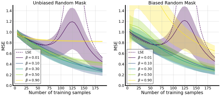
((a)) Regression task

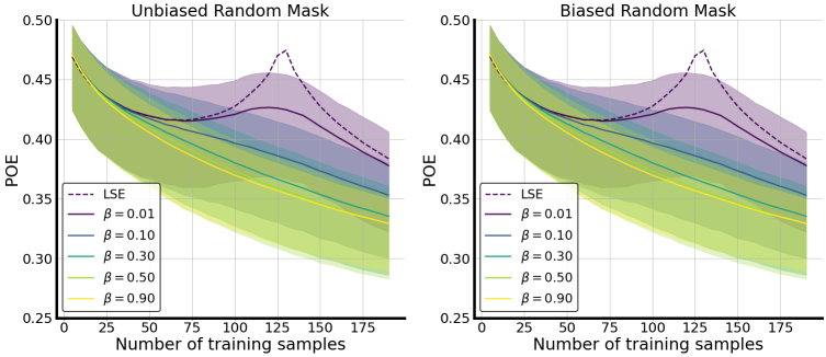
((b)) Classification task

Figure 3: Comparison of bias impact between regression and classification tasks In this figure, we simulate the unbiased and biased random mask in regression and classification tasks. In (a), we show that the augmentation bias is mostly harmful to the regression task, especially in the overparameterized regime where the sample number is less than or equal to $p=128$. In (b), however, the performance is identical with and without bias in the classification task. This verifies the very different conclusions from Theorems 7 and 11.

Data augmentation is easier to tune in classification than regression.

The results of Muthukumar et al. (2021) showed that the choice of test loss function critically impacts generalization. Specifically, they discovered that for the least squared estimator (LSE), there are cases where the model generalizes well for the classification task but not for regression. We complement this study by comparing generalization with DA in the two tasks. Specifically, we find that, for a given DA, the classification loss is always upper-bounded by a lower bound for the regression MSE, implying that regression is easier to train with DA than classification. Furthermore, we provide a concrete example of a simple class of augmentations for which the regression MSE is constant, but the classification POE is asymptotically zero. Our findings are summarized in the following proposition. The proof can be found in Appendix D.1.

Proposition 20 (DA is easier to tune in classification than regression).

Consider the 1-sparse model $\boldsymbol{\theta}^{*}=\sqrt{\frac{1}{\lambda_{t}}}\mathbf{e}_{t}$ for Gaussian covariate with independent components and an independent feature augmentation. Suppose that the approximation error is not dominant in the bounds of Theorem 4 (simple sufficient conditions can be found in Lemma 35 in Appendix A), and the assumptions in the two theorems hold. Then, we have

$$\mathrm{POE}(\hat{\boldsymbol{\theta}}_{\text{aug}}) \lesssim\sqrt{(\lambda_{k+1}^{\text{aug}}\rho_{k}({\boldsymbol{\Sigma}}_{\text{aug}};n))^{2}\cdot\left(\frac{n}{R_{k}({\boldsymbol{\Sigma}}_{\text{aug}};n)}+\frac{k}{n}\right)\log n},$$

$$\mathrm{MSE}(\hat{\boldsymbol{\theta}}_{\text{aug}}) \gtrsim(\lambda_{k+1}^{\text{aug}}\rho_{k}({\boldsymbol{\Sigma}}_{\text{aug}};n))^{2}+\left(\frac{n}{R_{k}({\boldsymbol{\Sigma}}_{\text{aug}};n)}+\frac{k}{n}\right).$$

As a consequence, the regression risk serves as a surrogate for the classification risk up to a $log$-factor:

$$\mathrm{POE}(\hat{\boldsymbol{\theta}}_{\text{aug}})\lesssim\mathrm{MSE}(\hat{\boldsymbol{\theta}}_{\text{aug}})\sqrt{\log n}.$$ (33)

To illustrate the implications of this proposition, let us consider the isotropic Gaussian noise injection augmentation with noise standard deviation $\sigma$ and random mask with dropout probability $\beta$ to train the 1-sparse model with a decaying data spectrum ${\boldsymbol{\Sigma}}_{ii}=\gamma^{i},\leavevmode\nobreak\ \forall i\in\{1,2,\dots,p\}$, where $\gamma$ is some constant satisfying $0<\gamma<1$. Let $\hat{\boldsymbol{\theta}}_{\text{gn}}$ and $\hat{\boldsymbol{\theta}}_{\text{rm}}$ be the corresponding estimators. Then, a direct consequence of Proposition 20 yields

$$\lim_{n\rightarrow\infty}\lim_{\sigma\rightarrow\infty}\mathrm{POE}(\hat{\boldsymbol{\theta}}_{\text{gn}})=0\leavevmode\nobreak\ \leavevmode\nobreak\ \text{while}\leavevmode\nobreak\ \leavevmode\nobreak\ \lim_{n\rightarrow\infty}\lim_{\sigma\rightarrow\infty}\mathrm{MSE}(\hat{\boldsymbol{\theta}}_{\text{gn}})=1.$$ (34)

Also, when $p\log n\ll n$,

$$\lim_{n\rightarrow\infty}\lim_{\beta\rightarrow 1}\mathrm{POE}(\hat{\boldsymbol{\theta}}_{\text{rm}})=0\leavevmode\nobreak\ \leavevmode\nobreak\ \text{while}\leavevmode\nobreak\ \leavevmode\nobreak\ \lim_{n\rightarrow\infty}\lim_{\beta\rightarrow 1}\mathrm{MSE}(\hat{\boldsymbol{\theta}}_{\text{rm}})=1.$$ (35)

(34) and (35) show that for both Gaussian noise injection and random mask augmentation, extreme augmentations can achieve perfect generalization in classification but poor generalization in regression.

It is worth noting that (34) in particular studies an augmentation that significantly changes the data distribution. In particular, for Gaussian injection augmentations we have

$$\frac{W^{2}_{2}(g(\mathbf{x}),\mathbf{x})}{p}\longrightarrow\infty\text{ as }n,\sigma\to\infty,$$ (36)

where $W_{2}$ denotes the 2-Wasserstein distance between the pre- and post-augmented distribution of the data by the Gaussian noise injection. In Figs. 6(b) and (d), we compare the Gaussian injection augmentation in the decaying spectrum $\gamma=0.95$ for regression and classification, respectively. We observe a sharp difference between classification and regression, where, as we increase the augmentation intensity (i.e. variance of injected Gaussian noise), the MSE increases while the POE converges to a stable value (the ratio between SU and CN stays the same), implying that careful tuning is required for regression but not for classification.

Our second example that illustrates special benefits of DA in classification over regression concerns non-uniform random masking. The proof of the following proposition is deferred to Appendix D.2.

Proposition 21 (Non-uniform random mask is easier to tune in classification than regression).

Consider the 1-sparse model $\boldsymbol{\theta}^{*}=\sqrt{\frac{1}{\lambda_{t}}}\mathbf{e}_{t}$. Suppose the approximation error is not dominant in the bounds of Theorem 4 (simple sufficient conditions can be found in Lemma 35in Appendix A) and the assumptions in the two theorems hold. Suppose we apply the non-uniform random mask augmentation and recall the definitions of $\psi$ and $\psi_{t}$ as in Corollary 45. Then, if $\sqrt{\frac{p}{n}}\ll\frac{\psi}{\psi_{t}}\ll\frac{p}{n},$ we have

$$\mathrm{POE}(\hat{\boldsymbol{\theta}}_{\text{rm}})\overset{n}{\longrightarrow}0\leavevmode\nobreak\ \leavevmode\nobreak\ \text{while}\leavevmode\nobreak\ \leavevmode\nobreak\ \mathrm{MSE}(\hat{\boldsymbol{\theta}}_{\text{rm}})\overset{n}{\longrightarrow}1.$$ (37)

By allowing the augmentation parameters $\psi$ and $\psi_{1}$ to vary with $n$, the induced spectrum ${\boldsymbol{\Sigma}}_{\text{aug}}$ recovers the “bi-level” design, which was shown in Theorem 13 of Muthukumar et al. (2021) to separate classification and regression performance. It is worth noting that in the case where the true sparsity pattern is known, several augmentations (including nonuniform Gaussian noise injection, which incurs no approximation error in our analysis) can give rise to the same consistency behavior described above.

As a takeaway, the corollaries in this section demonstrate that the choice of augmentation itself can be more benign for classification tasks. Specifically, augmentations that are “biased on average” may perform similarly to their unbiased counterparts; we cannot generally expect this behavior for regression. Finally, we concluded this section by showing that our framework can be applied to strongly out-of-distribution (OOD) augmentations, and show that strong distributional shift can sometimes lead to improvements in classification generalization. We observe the same phenomenon empirically in Fig. 6, where increasing the intensity of the augmentation improves generalization and also increases the distributional shift.

6 Experiments

In this section, we complement our theoretical analysis with empirical investigations. In particular, we explore: 1. Differences between aSGD which is used in practice and the closed-form aERM solution analyzed in this paper, 2. Comparisons between the generalization of different types of augmentations studied in this work, 3. Multiple factors that influence the efficacy of DA, including signal structure and covariate spectrum, and 4. Comparisons between different augmentation strategies, namely precomputed augmentations versus aERM. We provide our Python implementations in https://github.com/nerdslab/augmentation-theory.

6.1 Convergence of aSGD solution to the closed-form solution

In this paper, we mathematically study a-ERM (the solution in Equation (2)); however, the solution used in practice is obtained by running a-SGD (Algorithm 1). In this set of experiments, we investigate the convergence of Algorithm 1 to the solution of Eq. 2 to verify that our theory reflects the solutions obtained in practice. To this end, we use an example in the overparameterized regime with $p=128\geq n=64$ with the random isotropic signal $\boldsymbol{\theta}^{*}\sim\mathcal{N}(\mathbf{0},\mathbf{I}_{p})$ and the observation noise $\epsilon\sim\mathcal{N}(0,0.25)$. We choose a decaying covariate spectrum of the form ${\boldsymbol{\Sigma}}_{ii}\propto\gamma^{i}$, where $\gamma$ is chosen such that $\mu_{p}({\boldsymbol{\Sigma}})=0.6\mu_{1}({\boldsymbol{\Sigma}})$. We want to understand the interplay between the convergence rate of aSGD with batch and augmentation size (formally, the augmentation size is the number of augmentations made for each draw of the training examples). We run the aSGD algorithm with different batch sizes and augmentation sizes in the range given by $(64,1),(32,2),\dots,(2,32),(1,64)$. Note that the computation cost is proportional to the (batch size) $\times$ (augmentation size) per backward pass. Fig. 4 illustrates the convergence rate in terms of the number of backward passes. We observe that the convergence rates are fairly robust to different choices of batch and augmentation sizes.

input :  Data $\mathbf{x}_{i},\leavevmode\nobreak\ i=1,\dots,n$; Learning rates $\eta_{t},\leavevmode\nobreak\ t=1,\dots$; transformation distribution $\mathcal{G}$; batch size B; aug size H;

init $\hat{\boldsymbol{\theta}}\leftarrow\hat{\boldsymbol{\theta}}_{0}$

      

while termination condition not satisfied do

       for k=1,…,$\frac{\texttt{n}}{\texttt{B}}$ do

             for i=1,…,B in the batch $\mathcal{B}_{k}$ do

                   Draw H augmentations $g_{ij}\sim\mathcal{G}$, $j=1,\dots,$H

             end for

            $\hat{\boldsymbol{\theta}}_{t+1}\leftarrow\hat{\boldsymbol{\theta}}_{t}-\eta_{t}\sum\limits_{i=1}^{B}\sum\limits_{j=1}^{H}\nabla_{\boldsymbol{\theta}}(\langle\boldsymbol{\theta},g_{ij}(\mathbf{x}_{i})\rangle-y_{i})_{2}^{2}|_{\boldsymbol{\theta}=\hat{\boldsymbol{\theta}}_{t}}$

       end for

      

end while

Algorithm 1    Augmented Stochastic Gradient Descent (aSGD)

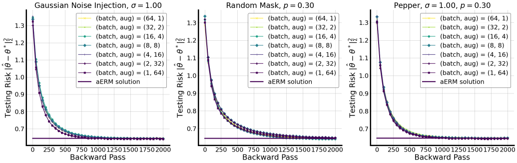
Figure 4: Convergence of augmented stochastic gradient descent (a-SGD, Algorithm 1) as a function of the number of backward passes to the closed-form solution of the a-ERM objective (Equation (2)). The result shows fairly stable convergence across different batch sizes and augmentation copies per sample.

A remark on the implicit bias of minimal or “weak" DA:

It is well-known that Gaussian noise injection approximates the LSE when the variance of the added noise approaches zero. Surprisingly, however, this does not imply that all kinds of DA approach the LSE in the limit of decreasing augmentation intensity. Suppose that the augmentation $g$ is characterized by some hyperparameter $\xi$ that reflects the intensity of the augmentation (for e.g., mask probability $\beta$ in the case of randomized mask, or Gaussian noise standard deviation $\sigma$ in the case of Gaussian noise injection), and that $\operatorname{Cov}_{G}(\mathbf{X})/\xi{\longrightarrow}\operatorname{Cov}_{\infty}$ as $\xi\rightarrow 0$ for some positive semidefinite matrix $\operatorname{Cov}_{\infty}$ that does not depend on $\xi$. Then, the limiting estimator when the augmentation intensity $\xi$ approaches zero is given by

$$\hat{\theta}_{aug}\overset{\xi\rightarrow 0}{\longrightarrow}\operatorname{Cov}_{\infty}^{-1}\mathbf{X}^{\top}\left(\mathbf{X}\operatorname{Cov}_{\infty}^{-1}\mathbf{X}^{\top}\right)^{\dagger}\mathbf{y}.$$ (38)

It can be easily checked that this estimator is the minimum-Mahalanobis-norm interpolant of the training data where the positive semi-definite matrix used for the Mahalanobis norm is given by $\operatorname{Cov}_{\infty}$. Formally, the estimator solves the optimization problem

$$\min_{\boldsymbol{\theta}}\|\boldsymbol{\theta}\|_{\operatorname{Cov}_{\infty}}\leavevmode\nobreak\ \leavevmode\nobreak\ {\text{s.t. }\mathbf{X}\boldsymbol{\theta}=\mathbf{y}}$$ (39)

Thus, the choice of augmentation impacts the specific interpolator that we obtain in the limit of minimally applied DA. For example, the above formula can be applied to random mask with

$$\operatorname{Cov}_{\infty}=n^{-1}\text{diag}(\mathbf{X}^{T}\mathbf{X})\approx{\boldsymbol{\Sigma}}.$$

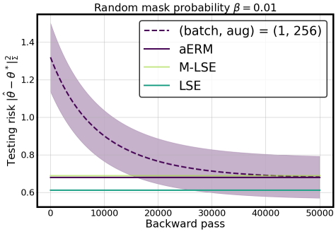
Figure 5: aSGD convergence to aERM for small random mask. We simulate the convergence of aSGD for random mask with dropout probability $0.01$. We compare its converging estimator with the aERM limit (38)).

Fig. 5 demonstrates that the MSE of the random mask does not converge to that of the LSE. Instead, it converges to the light green curve which we abbreviate as M-LSE (for the masked least squared estimator). To test whether these limits appear only in an aERM solution, we plot the convergence path of aSGD with the random mask augmentation with masking probability $\beta=0.01$. We set the ambient dimension $p$, noise standard deviation $\sigma_{\epsilon}$, number of training examples $n$, and learning rate $\eta$ to be $128$, $0.5$, $64$ and $10^{-5}$ respectively. We choose a decaying covariate spectrum of the form ${\boldsymbol{\Sigma}}_{ii}\propto\gamma^{i}$, where $\gamma$ is chosen such that $\mu_{p}({\boldsymbol{\Sigma}})=0.2\mu_{1}({\boldsymbol{\Sigma}})$. It is clear from the plot that both aSGD and aERM converges to the M-LSE solution of (38)). The curves and the shaded area denote the averaged result and the $90\%$ confidence interval for $50$ experiments. A caveat to this result is that the convergence rate turns out to be relatively slow and highly sensitive to the learning rate. A theoretical investigation of this behavior (and the optimization convergence of aSGD to aERM more generally) is beyond the scope of this work and would be interesting to explore in the future.

6.2 Comparisons of different types of augmentations

In this section, we compare the generalization of three canonical augmentations that we analyzed in this work: 1) Gaussian noise injection (Bishop, 1995), 2) random mask (He et al., 2022), and 3) random rotation (which we introduced in Section 3.4). As in Section 6.1, we consider the random isotropic signal $\boldsymbol{\theta}^{*}\sim\mathcal{N}(\mathbf{0},\mathbf{I}_{p})$. We compare regression and classification tasks; in the former, we set the noise standard deviation as $\sigma_{\varepsilon}=0.5$ while in the latter, we set the label noise parameter as $\nu^{*}=0.1$. We consider diagonal covariance ${\boldsymbol{\Sigma}}$ and two choices of spectrum: 1. isotropic (i.e. ${\boldsymbol{\Sigma}}=\mathbf{I}_{p}$) and 2. decaying spectrum where $\Sigma_{ii}\propto\gamma^{i}$ with $\gamma=0.95$.

Figure 6 illustrates different trade-offs (bias/variance for regression, contamination/survival for classification) for the three canonical augmentations. The hyperparameters for the respective augmentations are: 1) the standard deviation $\sigma\in\mathbb{R}^{+}$ of the Gaussian noise injection, 2) the masking probability $\beta\in[0,1]$ of the random mask, and 3) the rotation angle $\alpha\in[0,90]$. We can make the following observations from Figure 6:

1. For isotropic data, all three augmentations achieve similar results in terms of generalization, while for the case of decaying spectrum, Gaussian injection and random rotation outperform the random mask when their respective hyperparameters are all optimally tuned.

2. In the regression task, for both choices of data distribution, Gaussian injection requires careful hyperparameter tuning in the range of $[0,1.8]$ from $\mathbb{R}^{+}$ while the random mask and random rotation augmentations are fairly robust in performance in the entire range of the hyperparameter spaces. A possible explanation for this observation is that the random mask and rotation hyperparameters are scale free of the data (while the noise injection hyperparameter is not).

3. In the classification task, all the augmentations enjoy robust generalization guarantees with respect to their hyperparameters. This verifies our theoretical observations in Propositions 20 and 21.

4. While noise injection enjoys better generalization when it is optimally tuned, random mask is more robust in terms of generalization across hyperparameter choice. Our novel random rotation augmentation achieves the best of both worlds across different data distributions and tasks. In particular, it not only achieves a comparable generalization guarantee to noise injection when optimally tuned, but also is robust with respect to hyperparameter choice (like the random mask). This observation is consistent with the theoretical prediction of Corollary 19.

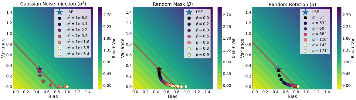
((a)) Bias and variance distribution comparison in uniform covariate spectrum.

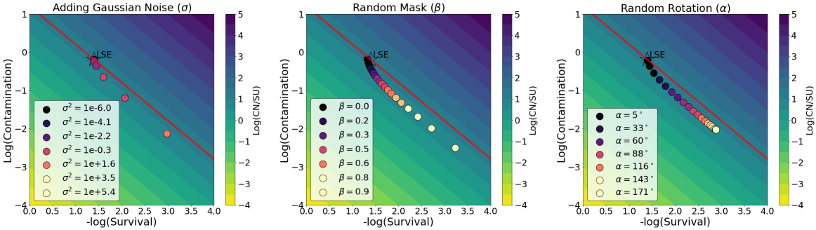
((b)) Log survival and contamination distribution comparison in uniform covariate spectrum.

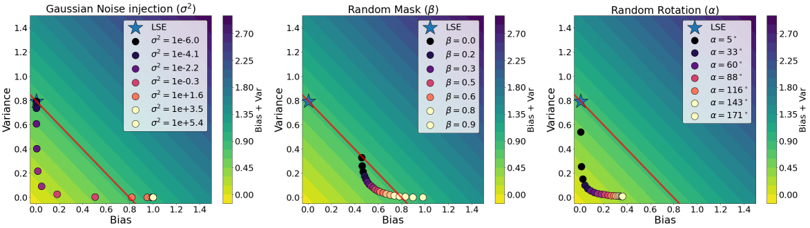
((c)) Bias and variance distribution comparison in decaying covariate spectrum, $\gamma=0.95$

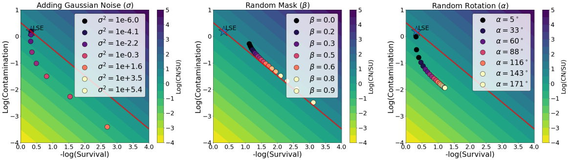
((d)) Log survival and contamination distribution comparison in decaying covariate spectrum, $\gamma=0.95$

Figure 6: Adding Gaussian Noise vs. Random Mask v.s Random Rotation in different covariate spectra for the regression and classification tasks. In this figure we plot the bias/variance (a), (c) and contamination/survival distributions (b), (d) of Gaussian noise injection, random mask, and random rotation. The numbers reflect the respective hyperparameters $\sigma,\beta,\alpha$.

6.3 When are augmentations effective?

In this section, we try to understand the impact of the true model $\boldsymbol{\theta}^{*}$ and the data covariance ${\boldsymbol{\Sigma}}$ on the efficacy of different augmentations, focusing on the nonuniform random mask introduced in Section 5.2.2. We set the ambient dimension to $p=128$ and consider the noise standard deviation $\sigma_{\epsilon}=0.5$.

Effect of true model

We study the impact of nonuniform masking on the 1-sparse model $\boldsymbol{\theta}^{*}=\mathbf{e}_{1}$, as depicted in Section 4.1 in the regression task and consider isotropic covariance ${\boldsymbol{\Sigma}}=\mathbf{I}_{p}$. We vary the probability of the signal feature mask $\beta_{sig}$ while keeping the probability of the noise feature mask $\beta$ fixed at $0.2$. The results are summarized in Fig. 7 and verify our analysis in Corollary 18 that noise features should be masked more compared to signal features so that the semantic component in the data is preserved. Furthermore, we observe that the differences manifest primarily in the bias, and the variance remains roughly the same. This is consistent with our variance bound in Corollary 18, which depends only on the probability of the noise mask $\beta$.

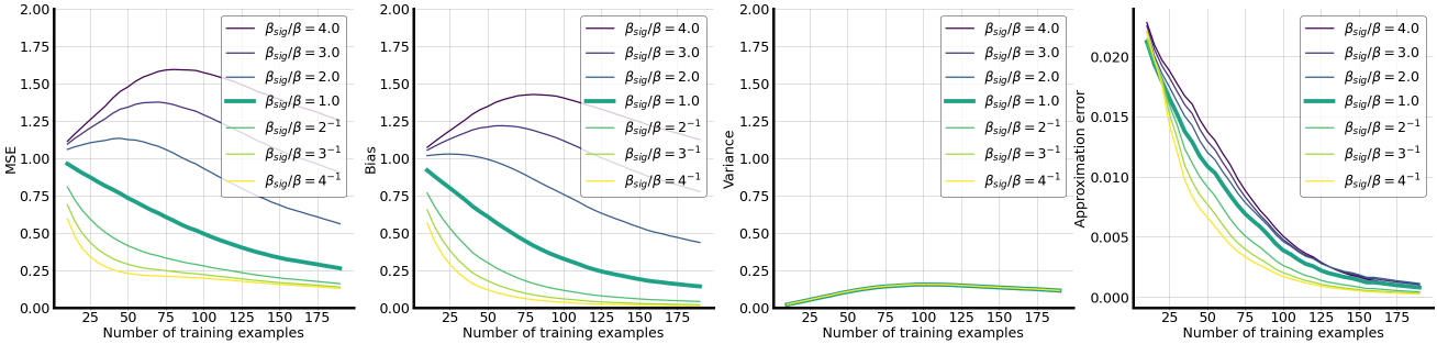
Figure 7: Non-uniform random mask between signal and noise features. We illustrate different mask strategies by varying the relative mask intensities of the signal and noise features. We see the signal position on the true model has most impact on the bias for data augmentation. Furthermore, the result supports the principle that one should augment the noise features more than the signal feature.

Effect of covariate spectrum

Next, to understand the impact of the covariate spectrum, we consider a setting with a decaying data spectrum ${\boldsymbol{\Sigma}}_{ii}\propto 0.95^{i}$. We generate the true model using the random isotropic Gaussian $\boldsymbol{\theta}^{*}\sim\mathcal{N}(0,\mathbf{I}_{p})$ and run the experiment $100$ times, reporting the average result. We consider a bilevel masking strategy where the masking probability for the first half of features is set to $\beta_{1}$, and the second half of features is set to $\beta_{p}$. We vary the ratio between $\beta_{p}$ and $\beta_{1}$ to investigate whether a feature with larger eigenvalue should be augmented with stronger intensity or not. The result is presented in Fig. 8. We observe from this figure that it is more beneficial to augment more for features with smaller eigenvalues.

Figure 8: Impact of covariance spectrum on the random mask in $p=128$ dimensions. We investigate the bi-level random mask strategies in data with decaying spectrum $\propto 0.95^{i}$. The first half of features are masked with probability $\beta_{1}$ while the rest are with $\beta_{p}$. We vary the ratio between the intensity $\beta_{p}/\beta_{1}$. We observe that augmenting more for features with higher variance benefits generalization.

6.4 Comparisons of pre-computing samples vs. augmented ERM

In our final set of experiments, we dig into the differences between pre-computing augmented samples and creating augmentations on the fly (our analysis concerns the latter). Because modern deep learning training usually relies on GPU computation, the overhead of doing augmentation with CPU on the fly with optimization could become a bottleneck during training time. Hence, pre-processing of the data becomes a plausible alternative. This is essentially equivalent to optimizing an empirical notion of aERM:

$$\frac{1}{\text{aug size}}\sum_{i=1}^{\text{aug size}}[\|G_{i}(\mathbf{X})-\mathbf{y}\|_{2}^{2}]=\hat{\mathbb{E}}_{G}[\|G(\mathbf{X})-\mathbf{y}\|_{2}^{2}].$$ (40)

For this experiment, we generate isotropic random signal $\boldsymbol{\theta}^{*}\sim\mathcal{N}(\mathbf{0},\mathbf{I}_{128})$ and observation noise with standard deviation $\sigma=0.5$. For simplicity, we choose the isotropic covariate spectrum ${\boldsymbol{\Sigma}}=\mathbf{I}_{128}$. Fig. 9 shows regression performance in terms of MSE, bias, and variance as we vary the augmentation size, which is the number of augmented copies of each original sample. In Figs. 9 (a)-(b), we observe the well-known double descent peaks (Belkin et al., 2020; Nakkiran et al., 2020) when the training number approaches the ambient dimension $n=p=128$ for LSE, and observe that adding pre-computed augmentation shifts these peaks to the left. The peak for a pre-computing method with an augmentation size $k$ is observed to be approximately at $n=128/k$. Intuitively, this mode of augmentation virtually increases the size of the training data: in particular, if we had $128/k$ original data points the induced total training size (including original data points and augmentations) becomes equal to $(128/k)\times k=128$.

Interestingly, both the magnitude of the peak and the width decrease as we increase the augmentation size, and the peak almost disappears when $k>8$. The general behavior of pre-computing is observed to approach aERM as $k$ increases. Another interesting observation is that, unlike LSE which only has a double descent peak in the variance, pre-computing augmentations induces peaks in both the bias and the variance. A possible explanation for peaks appearing even in the bias term is that the variance induced by a finite number of augmentations is itself embedded in the bias term. In more detail: let $\hat{\boldsymbol{\theta}}_{\text{aug}}=\hat{\boldsymbol{\theta}}_{\text{aug}}(\varepsilon,g,\mathbf{X})$ be the augmentation estimator that depends on the observation noise $\varepsilon$, finite augmentation $g$, and training data $\mathbf{X}$. Then the bias term can be decomposed as

$$\underbrace{\|\hat{\boldsymbol{\theta}}_{\text{aug}}-\mathbb{E}_{\varepsilon}[\hat{\boldsymbol{\theta}}_{\text{aug}}|\mathbf{X}]\|^{2}_{\boldsymbol{\Sigma}}}_{\mathrm{Bias}}\leavevmode\nobreak\ \lesssim\leavevmode\nobreak\ \underbrace{\|\hat{\boldsymbol{\theta}}_{\text{aug}}-\mathbb{E}_{g,\varepsilon}[\hat{\boldsymbol{\theta}}_{\text{aug}}|\mathbf{X}]\|^{2}_{\boldsymbol{\Sigma}}}_{\mathrm{Average\leavevmode\nobreak\ augmentation\leavevmode\nobreak\ bias}}\leavevmode\nobreak\ +\leavevmode\nobreak\ \underbrace{\|\mathbb{E}_{\varepsilon}[\hat{\boldsymbol{\theta}}_{\text{aug}}|\mathbf{X}]-\mathbb{E}_{g,\varepsilon}[\hat{\boldsymbol{\theta}}_{\text{aug}}|\mathbf{X}]\|^{2}_{\boldsymbol{\Sigma}}}_{\mathrm{Finite\leavevmode\nobreak\ augmentation\leavevmode\nobreak\ variance}}.$$

We defer a detailed mathematical study of these intriguing observations to future work.

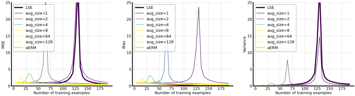
((a)) Normal adding Gaussian noise with $\sigma=1$.

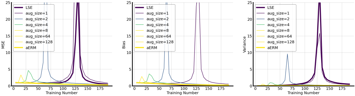
((b)) Normal random mask with $\beta=0.3$.

Figure 9: Pre-augmentation versus aERM in Gaussian Noise Injection and Random Mask. The estimators based on aERM have monotonicity in generalization error with respect to the number of training samples, while the pre-computing methods exhibit the double-descent phenomenon like least-squared estimators. We note that the pre-computing methods shifts the error peak left compared with LSE. Also, the peak appears approximately at the sample number equals to $\frac{p}{k}$, where $k$ is the augmentation size.

7 Discussion

In this paper, we establish a new framework to analyze the generalization error of the linear model with data augmentation in underparameterized and overparameterized regimes. We characterize generalization error for both regression and classification tasks in terms of the interplay between the characteristics of the data augmentation and spectrum of the data covariance. As a side product, our results also generalize the recent line of research on harmless interpolation from ridge/ridgeless regression to settings where the learning objectives are penalized by data dependent regularizers. Through our analysis, we characterize when a DA can help or hurt generalization based on the effective ranks of the augmented data spectrum. As concrete case studies, we show that in the overparametrized regime, random mask and group invariant augmentations can be harmful due to their isotropizing effect; on the other hand, our proposed random rotation augmentation is provably beneficial for generalization and highly robust. Our framework also uncovers the nuanced impact of DA on generalization as multiple factors, including the operating regimes, downstream tasks, and signal positions, come into play. We find that generalization can exhibit huge discrepancies even when the same type of DA has been employed.

There are several promising future directions that arise from our work. A first natural question is to what extent our insights extend to the nonlinear realm. A near-term future direction consists of extending our framework to kernel methods, which is often regarded as the first step toward understanding complex nonlinear models. As remarked at through various points in this paper, we believe the generalization analysis for a fixed estimator can be naturally extended; the more interesting question lies in the understanding the regularizer and estimator induced by DA for kernel models (that remain linear in feature-space but can be highly nonlinear in the data). Second, while our work focuses on the aERM objective, pre-computing augmentations is a natural alternative for which our preliminary experiments in Section 6.4 show intriguing differences in behavior. Understanding the fundamental differences between the two paradigms is an essential next step in comprehensively characterizing the effects of DA.

Appendix

.tocmtappendix mtchapternone mtappendixsubsection

Contents

1. 1 Introduction
   1. 1.1 Main contributions
2. 2 Related work
   1. 2.1 Data augmentation
   2. 2.2 Interpolation and regularization in overparameterized models
3. 3 Problem Setup
   1. 3.1 Empirical risk minimization with data augmentation
   2. 3.2 Implications of a DA-induced regularizer and connections to ridge regression
   3. 3.3 Practically used augmentations
   4. 3.4 Novel augmentation design
4. 4 Main Results
   1. 4.1 Preliminaries
      1. 4.1.1 Error Metrics
      2. 4.1.2 Spectral quantities of interest
   2. 4.2 A deterministic approximation strategy for DA analysis
   3. 4.3 Regression analysis
      1. 4.3.1 Regression analysis for general classes of unbiased augmentations
      2. 4.3.2 Regression analysis for general biased on average augmentations
   4. 4.4 Classification analysis
      1. 4.4.1 Classification analysis setup
      2. 4.4.2 Classification analysis for unbiased augmentations
      3. 4.4.3 Classification analysis for general biased augmentations
5. 5 The good, the bad and the ugly sides of data augmentation
   1. 5.1 Case studies: generalization of common DA
      1. 5.1.1 Gaussian noise injection
      2. 5.1.2 Randomized masking
      3. 5.1.3 Random cutout
      4. 5.1.4 Composite augmentation: Salt-and-pepper
   2. 5.2 The good and bad of DA: when is it helpful or harmful?
      1. 5.2.1 The bad: the increase in bias might outweigh the variance reduction
      2. 5.2.2 The good: some types of DA are superior to ridge regularization
      3. 5.2.3 Using our framework as a test bed for new DA
   3. 5.3 The ugly: discrepancies in DA’s effect under multiple factors
6. 6 Experiments
   1. 6.1 Convergence of aSGD solution to the closed-form solution
   2. 6.2 Comparisons of different types of augmentations
   3. 6.3 When are augmentations effective?
   4. 6.4 Comparisons of pre-computing samples vs. augmented ERM
7. 7 Discussion
8. A General Auxiliary Lemmas
9. B Proofs of Regression Results
   1. B.1 Regression Lemmas
   2. B.2 Proof of Theorem 4
   3. B.3 Proof of Theorem 7
   4. B.4 Proof of Proposition 5
   5. B.5 Proofs of Corollaries
10. C Proofs of Classification Results
    1. C.1 Classification Lemmas
    2. C.2 Proof of Theorem 9
    3. C.3 Proof of Theorem 11
    4. C.4 Proofs of Corollaries
11. D Comparisons between Regression and Classification
    1. D.1 Proof of Proposition 20
    2. D.2 Proof of Proposition 21
12. E Derivations of Common Augmented Estimators
13. F Approximation Error for Dependent Feature Augmentation
    1. F.1 Approximation error of random rotations
    2. F.2 Approximation error of random cutout

Appendix A General Auxiliary Lemmas

Notation

For a data matrix $\mathbf{X}\in\mathbb{R}^{n\times p}$ with i.i.d. rows with covariance ${\boldsymbol{\Sigma}}$, recall we denote $\mathbf{P}^{{\boldsymbol{\Sigma}}}_{1:k-1}$ and $\mathbf{P}^{{\boldsymbol{\Sigma}}}_{k:\infty}$ as the projection matrices to the first $k-1$ and the remaining eigen-subspaces of ${\boldsymbol{\Sigma}}$, respectively. In addition, we have defined two effective ranks $\rho_{k}({{\boldsymbol{\Sigma}}};c)=\frac{c+\sum_{i>k}\lambda_{i}}{n\lambda_{k+1}},\leavevmode\nobreak\ \leavevmode\nobreak\ R_{k}({{\boldsymbol{\Sigma}}};c)=\frac{(c+\sum_{i>k}\lambda_{i})^{2}}{\sum_{i>k}\lambda_{i}^{2}}.$ For convenience, we denote the residual Gram matrix by $\mathcal{A}_{k}(\mathbf{\mathbf{X}};\lambda)=\lambda\mathbf{I}_{n}+\mathbf{\mathbf{X}}\boldsymbol{P}^{{\boldsymbol{\Sigma}}}_{k:\infty}\mathbf{\mathbf{X}}^{T}$.

Lemma 22 (An useful identity for the ridge estimator (Tsigler and Bartlett, 2020)).

For any matrix $\mathbf{V}\in\mathbb{R}^{p\times k}$ composed of $k$ independent orthonormal columns (therefore, $\mathbf{V}$ represents a $k$-dimensional subspace), the ridge estimator $\hat{\boldsymbol{\theta}}=(\mathbf{X}^{\top}\mathbf{X}+\lambda\mathbf{I}_{p})^{\top}\mathbf{X}^{\top}\mathbf{y}$ has the property:

$$(\mathbf{I}_{k}+\mathbf{V}^{\top}\mathbf{X}^{\top}\mathbf{P}_{k}^{-1}\mathbf{X}\mathbf{V})\mathbf{V}^{\top}\hat{\theta}=\mathbf{V}^{\top}\mathbf{X}^{\top}\mathbf{P}_{k}^{-1}\mathbf{y},$$ (41)

where $\mathbf{P}_{k}:=\lambda\mathbf{I}_{n}+\mathbf{\mathbf{X}}\mathbf{V}^{\perp}(\mathbf{V}^{\perp})^{\top}{\mathbf{X}}^{\top}$ and $\mathbf{V}^{\perp}$ is a $p$ by $p-k$ matrix satisfying $(\mathbf{V}^{\perp})^{\top}\mathbf{V}=\mathbf{0}$ and $(\mathbf{V}^{\perp})^{\top}\mathbf{V}^{\perp}=\mathbf{I}_{p-k}$.

Lemma 23 (Bernstein-type inequality for sum of sub-exponential variables).

Let $\mathbf{x}_{1},\ldots,\mathbf{x}_{n}$ be independent zero-mean sub-exponential random variables with sub-exponential norm at most $\sigma_{x}^{2}$. Then for every $a=$ $\left(a_{1},\ldots,a_{n}\right)\in\mathbb{R}^{n}$ and every $t\geq 0$, we have

$$\mathbb{P}\left\{\left|\sum_{i=1}^{n}a_{i}\mathbf{x}_{i}\right|\geq t\right\}\leq 2\exp\left[-c\min\left(\frac{t^{2}}{\sigma_{x}^{4}\|a\|_{2}^{2}},\frac{t}{\sigma_{x}^{2}\|a\|_{\infty}}\right)\right]$$

where $c>0$ is an absolute constant.

Lemma 24 (Concentration of regularized truncated empirical covariance, Lemma 21 in Tsigler and Bartlett (2020)).

Suppose $\mathbf{Z}=[\mathbf{z}_{1},\mathbf{z}_{2},\dots,\mathbf{z}_{p}]\in\mathbb{R}^{n\times p}$ is a matrix with independent isotropic sub-gaussian rows with norm $\sigma$. Consider ${\boldsymbol{\Sigma}}=\operatorname{diag}\left(\lambda_{1},\ldots,\lambda_{p}\right)$ for some positive non-increasing sequence $\left\{\lambda_{i}\right\}_{i=1}^{p}$.

Denote $\mathbf{A}_{k}=\lambda\mathbf{I}_{n}+\sum_{i>k}\lambda_{i}\mathbf{z}_{i}\mathbf{z}_{i}^{\top}$ for some $\lambda\geq 0$. Suppose that it is known that for some $\delta,L>0$ independent of $n,p$ and some $k<n$ with probability at least $1-\delta$, the condition number of the matrix $\mathbf{A}_{k}$ is at most L. Then, for some absolute constant $c$ with probability at least $1-\delta-2\exp(-ct)$

$$\frac{(n-t\sigma^{2})}{L}\lambda_{k+1}\rho_{k}({\boldsymbol{\Sigma}};\lambda)\leq\mu_{n}\left(\mathbf{A}_{k}\right)\leq\mu_{1}\left(\mathbf{A}_{k}\right)\leq{\left(n+t\sigma^{2}\right)L\lambda_{k+1}}\rho_{k}({\boldsymbol{\Sigma}};\lambda)$$

Lemma 25 (Concentration of leave-one-out empirical covariance).

Under the same notations and assumptions in Lemma 24, denote $\mathbf{A}_{-t}:=\lambda\mathbf{I}_{n}+\sum_{i\neq t}\lambda_{i}\mathbf{z}_{i}\mathbf{z}_{i}^{\top}$ for some $\lambda\geq 0$. Then for any $t\leq k\leq n$ such that the condition number of $\mathbf{A}_{k}$ is bounded by $L$, we have

$$\frac{(n-t\sigma^{2})}{L}\lambda_{k+1}\rho_{k}({\boldsymbol{\Sigma}};\lambda)\leq\mu_{n}(\mathbf{A}_{-t})\leq\mu_{1}(\mathbf{A}_{-t})\leq{\left(n+t\sigma^{2}\right)L\lambda_{1}}\rho_{0}({\boldsymbol{\Sigma}};\lambda)$$

Proof  The lemma follows by Lemma 24 and the observations of $\mu_{1}(\mathbf{A}_{-t})\leq\mu_{1}(\mathbf{A}_{0}))$ and $\mathbf{A}_{-t}\succeq\mathbf{A}_{k}$.  

Lemma 26 (Concentration of matrix with independent sub-gaussian rows, Theorem 5.39 in Vershynin (2010)).

Let $\mathbf{X}$ be an $n\times k$ matrix (with $n>k$) whose rows $\mathbf{x}_{i}$ are independent sub-gaussian isotropic random vectors in $\mathbb{R}^{k}$. Then for every $t\geq 0$ such that $\sqrt{n}-C\sqrt{k}-t>0$ for some constant $C>0$, we have with probability at least $1-2\exp\left(-ct^{2}\right)$ that

$$\sqrt{n}-C\sqrt{k}-t\leq s_{\min}(\mathbf{X})\leq s_{\max}(\mathbf{X})\leq\sqrt{n}+C\sqrt{k}+t$$

Here $s_{\min}$ and $s_{\max}$ denotes the minimum and maximum singular values and $C,c>0$ are some constants depend only on the sub-gaussian norm of the rows.

Lemma 27 (Concentration of the sum of squared norms, Lemma 17 in Tsigler and Bartlett (2020)).

Suppose $\mathbf{Z}\in\mathbb{R}^{n\times p}$ is a matrix with independent isotropic sub-gaussian rows with norm $\sigma$. Consider ${\boldsymbol{\Sigma}}=\operatorname{diag}\left(\lambda_{1},\ldots,\lambda_{p}\right)$ for some positive non-decreasing sequence $\left\{\lambda_{i}\right\}_{i=1}^{p}$. Then for some absolute constant $c$ and any $t\in(0,n)$ with probability at least $1-2\exp(-ct)$

$$\left(n-t\sigma^{2}\right)\sum_{i>k}\lambda_{i}\leq\sum_{i=1}^{n}\left\|{\boldsymbol{\Sigma}}_{k:\infty}^{1/2}\mathbf{Z}_{i,k:\infty}\right\|^{2}\leq\left(n+t\sigma^{2}\right)\sum_{i>k}\lambda_{i}$$

Lemma 28 (Applications of Hanson-Wright inequality as done in Muthukumar et al. (2021)).

Let $\mathbf{\varepsilon}$ be a random vector composed of $n$ i.i.d. zero-mean sub-gaussian variables with norm $1$. Then,

1. there exists universal constant $c>0$ such that for any fixed positive semi-definite matrix $\mathbf{\mathbf{A}}$, with probability $1-2\exp(-\sqrt{n})$, we have

$$\left|\mathbf{\varepsilon}^{\top}\mathbf{\mathbf{A}}\mathbf{\varepsilon}-\mathbb{E}\left[\mathbf{\varepsilon}^{\top}\mathbf{\mathbf{A}}\mathbf{\varepsilon}\right]\right|\leq c\|\mathbf{A}\|n^{\frac{3}{4}}.$$

2. there exists some universal constant $C>0$ such that with probability at least $1-\frac{1}{n}$

$$\varepsilon^{\top}\mathbf{A}\varepsilon\leq C\operatorname{tr}(\mathbf{A})\log n.$$

Lemma 29 (Operator norm bound of matrix with sub-gaussian rows (Tsigler and Bartlett, 2020)).

Suppose $\left\{\mathbf{z}_{i}\right\}_{i=1}^{n}$ is a sequence of independent sub-gaussian vectors in $\mathbb{R}^{p}$ with $\left\|\mathbf{z}_{i}\right\|\leq\sigma$. Consider ${\boldsymbol{\Sigma}}=\operatorname{diag}\left(\lambda_{1},\ldots,\lambda_{p}\right)$ for some positive non-decreasing sequence $\left\{\lambda_{i}\right\}_{i=1}^{p}.$ Denote $\mathbf{X}$ to be the matrix with rows ${\boldsymbol{\Sigma}}^{1/2}\mathbf{z}_{i}$. Then for some absolute constant $c$, for any $t>0$ with probability at least $1-4e^{-t/c}$

$$\|\mathbf{X}\|\leq c\sigma\sqrt{\lambda_{1}(t+n)+\sum_{j=1}^{p}\lambda_{j}}.$$

Appendix B Proofs of Regression Results

In this section, we will include essential lemmas in B.1 to prove the main theorems for regression analysis in the sections B.2 and B.3. Then, we will use these theorems to prove the propositions and corollaries in sections B.4 and B.5, respectively.

B.1 Regression Lemmas

Lemma 30 (Sharpened bias of ridge regression, extension of Tsigler and Bartlett (2020)).

$$\frac{\rm{Bias}}{C_{x}L_{1}^{4}} \lesssim{{\left\|\mathbf{P}^{{\boldsymbol{\Sigma}}}_{k_{1}+1:p}{\theta}^{*}\right\|_{{\boldsymbol{\Sigma}}}^{2}+\left\|\mathbf{P}^{{\boldsymbol{\Sigma}}}_{1:k_{1}}{\theta}^{*}\right\|_{{\boldsymbol{\Sigma}}^{-1}}^{2}\frac{\rho_{k_{1}}^{2}({\boldsymbol{\Sigma}};n)}{{(\lambda_{k_{1}+1})^{-2}}+(\lambda_{1})^{-2}\rho_{k_{1}}^{2}({\boldsymbol{\Sigma}};n)}}}$$ (42)

Remark 31.

The reason we modify the bound from Tsigler and Bartlett (2020) is twofold: 1. we consider non-diagonal covariance matrix ${\boldsymbol{\Sigma}}$. This is because even if the original data covariance is diagonal, the equivalent spectrum might become non-diagonal after the data augmentation. Therefore, we modify the bound so that the eigenspaces of the data covariance matrix do not have to be aligned with the standard basis. 2. As we show in our work, some augmentations, e.g. random mask, have the effect of making the equivalent data spectrum isotropic. However, in this case, the bias bound in Tsigler and Bartlett (2020), as shown below, can be vacuous as being almost the same as the null estimator so we modify the bound to remedy the case.

$$\rm{Bias\leavevmode\nobreak\ bound}\leavevmode\nobreak\ \asymp\leavevmode\nobreak\ {{\left\|\mathbf{P}^{{\boldsymbol{\Sigma}}}_{k_{1}+1:p}{\theta}^{*}\right\|_{{\boldsymbol{\Sigma}}}^{2}+\left\|\mathbf{P}^{{\boldsymbol{\Sigma}}}_{1:k_{1}}{\theta}^{*}\right\|_{{\boldsymbol{\Sigma}}^{-1}}^{2}{\lambda_{k_{1}+1}^{2}\rho_{k_{1}}^{2}({\boldsymbol{\Sigma}};n)}}}$$

$$\leavevmode\nobreak\ =\leavevmode\nobreak\ {{\left\|\mathbf{P}^{{\boldsymbol{\Sigma}}}_{k_{1}+1:p}{\theta}^{*}\right\|^{2}+\left\|\mathbf{P}^{{\boldsymbol{\Sigma}}}_{1:k_{1}}{\theta}^{*}\right\|^{2}\frac{p-k_{1}}{n}}}\gtrsim\|\boldsymbol{\theta}^{*}\|_{2}^{2},$$

Proof  This lemma is a modification to Theorem 1 in Tsigler and Bartlett (2020), where we only change slightly in the estimation of the lower tail of the bias. For self-containment, we illustrate where we make the change. Consider the diagonalization ${\boldsymbol{\Sigma}}=\mathbf{V}\mathbf{D}\mathbf{V}^{\top}$. Let $\mathbf{V}_{1},\leavevmode\nobreak\ \mathbf{V}_{2}$ be the matrices with columns consisting of the top $k$ eigenvectors of ${\boldsymbol{\Sigma}}$ and the remaining eigenvectors, respectively. Note that we have $\mathbf{V}=[\mathbf{V}_{1},\mathbf{V}_{2}]$, $\boldsymbol{P}^{{\boldsymbol{\Sigma}}}_{1:k-1}=\mathbf{V}_{1}\mathbf{V}_{1}^{\top},$ and $\boldsymbol{P}^{{\boldsymbol{\Sigma}}}_{k:\infty}=\mathbf{V}_{2}\mathbf{V}_{2}^{\top}$. Moreover, we have $\mathbf{V}_{1}\mathbf{V}_{1}^{\top}+\mathbf{V}_{2}\mathbf{V}_{2}^{\top}=\mathbf{V}\mathbf{V}^{\top}=\mathbf{I}_{p}$. Now, for the ridge estimator $\hat{\theta}=(\mathbf{X}^{\top}\mathbf{X}+\lambda\mathbf{I}_{p})^{-1}\mathbf{X}^{\top}\mathbf{y}$, apply Lemma 22 with $\mathbf{V}=\mathbf{V}_{1}$ to obtain

$$(\mathbf{I}_{k}+\mathbf{V}_{1}^{\top}\mathbf{X}^{\top}\mathcal{A}_{k}({\boldsymbol{\Sigma}};\lambda)^{-1}\mathbf{X}\mathbf{V}_{1})\mathbf{V}_{1}^{\top}\hat{\theta}=\mathbf{V}_{1}^{\top}\mathbf{X}^{\top}\mathcal{A}_{k}({\boldsymbol{\Sigma}};\lambda)^{-1}\mathbf{y},$$ (43)

where $\mathcal{A}_{k}({\boldsymbol{\Sigma}};\lambda):=\lambda\mathbf{I}_{p}+\mathbf{X}\mathbf{V}_{2}\mathbf{V}_{2}^{\top}\mathbf{X}^{\top}$. As there will be no ambiguity of which covariance matrix the residual spectrum corresponds to, we will just write $\mathbf{A}_{k}$ from now on.

To bound the bias, we split it into

$$\text{Bias}\leavevmode\nobreak\ {\leq}\leavevmode\nobreak\ 2\|\mathbf{V}_{1}\mathbf{V}_{1}^{\top}(\mathbb{E}_{\varepsilon}[\hat{\boldsymbol{\theta}}]-\boldsymbol{\theta}^{*})\|_{{\boldsymbol{\Sigma}}}^{2}+2\|\mathbf{V}_{2}\mathbf{V}_{2}^{\top}(\mathbb{E}_{\varepsilon}[\hat{\boldsymbol{\theta}}]-\boldsymbol{\theta}^{*})\|_{{\boldsymbol{\Sigma}}}^{2},$$ (44)

where the expectations are over the noise $\varepsilon$. Observe that the averaged estimator is $\mathbb{E}_{\varepsilon}[\hat{\boldsymbol{\theta}}]=(\mathbf{X}^{\top}\mathbf{X}+\lambda\mathbf{I}_{p})^{-1}\mathbf{X}^{\top}\mathbf{y}$, so we can apply Lemma 22 with $\hat{\boldsymbol{\theta}}$ and $\mathbf{y}$ replaced by $\mathbb{E}_{\varepsilon}[\hat{\boldsymbol{\theta}}]$ and $\mathbf{X}\boldsymbol{\theta}^{*}$, respectively. As a result, we can write

$$(\mathbf{I}_{k}+\mathbf{V}_{1}^{\top}\mathbf{X}^{\top}\mathbf{A}_{k}^{-1}\mathbf{X}\mathbf{V}_{1})\mathbf{V}_{1}^{\top}\mathbb{E}_{\varepsilon}[\hat{\boldsymbol{\theta}}]=\leavevmode\nobreak\ \mathbf{V}_{1}^{\top}\mathbf{X}^{\top}\mathbf{A}_{k}^{-1}\mathbf{X}\boldsymbol{\theta}^{*}$$

$$=\leavevmode\nobreak\ \mathbf{V}_{1}^{\top}\mathbf{X}^{\top}\mathbf{A}_{k}^{-1}\mathbf{X}(\mathbf{V}_{1}\mathbf{V}_{1}^{\top}+\mathbf{V}_{2}\mathbf{V}_{2}^{\top})\boldsymbol{\theta}^{*}.$$

Now, subtracting $\mathbf{V}_{1}^{\top}\boldsymbol{\theta}^{*}+\mathbf{V}_{1}^{\top}\mathbf{X}^{\top}\mathbf{A}_{k}^{-1}\mathbf{X}\mathbf{V}_{1}\mathbf{V}_{1}^{\top}\boldsymbol{\theta}^{*}$ from both sides of the above equation followed by a left multiplication of $\mathbf{V}_{1}$ gives

$$\mathbf{V}_{1}\mathbf{V}_{1}^{\top}(\mathbb{E}_{\varepsilon}\hat{\boldsymbol{\theta}}-\boldsymbol{\theta}^{*})+\mathbf{V}_{1}\mathbf{V}_{1}^{\top}\mathbf{X}^{\top}\mathbf{A}_{k}^{-1}\mathbf{X}\mathbf{V}_{1}\mathbf{V}_{1}^{\top}(\mathbb{E}_{\varepsilon}\hat{\boldsymbol{\theta}}-\boldsymbol{\theta}^{*})$$

$$=\mathbf{V}_{1}\mathbf{V}_{1}^{\top}\mathbf{X}^{\top}\mathbf{A}_{k}^{-1}\mathbf{X}\mathbf{V}_{2}\mathbf{V}_{2}^{\top}\boldsymbol{\theta}^{*}-\mathbf{V}_{1}\mathbf{V}_{1}^{\top}\boldsymbol{\theta}^{*},$$

where we use the identity $\mathbf{I}_{p}=\mathbf{V}_{1}\mathbf{V}_{1}^{\top}+\mathbf{V}_{2}\mathbf{V}_{2}^{\top}$.

Now multiply both sides with $(\mathbb{E}_{\varepsilon}\hat{\boldsymbol{\theta}}-\boldsymbol{\theta}^{*})^{\top}$, the R.H.S. is

$$=\leavevmode\nobreak\ \leavevmode\nobreak\ (\mathbb{E}_{\varepsilon}\hat{\boldsymbol{\theta}}-\boldsymbol{\theta}^{*})^{\top}\mathbf{V}_{1}\mathbf{V}_{1}^{\top}{\boldsymbol{\Sigma}}^{1/2}{\boldsymbol{\Sigma}}^{-1/2}\mathbf{X}^{\top}\mathbf{A}_{k}^{-1}\mathbf{X}\mathbf{V}_{2}\mathbf{V}_{2}^{\top}\boldsymbol{\theta}^{*}-(\mathbb{E}_{\varepsilon}\hat{\boldsymbol{\theta}}-\boldsymbol{\theta}^{*})^{\top}\mathbf{V}_{1}\mathbf{V}_{1}^{\top}{\boldsymbol{\Sigma}}^{1/2}{\boldsymbol{\Sigma}}^{-1/2}\boldsymbol{\theta}^{*}$$

$$\leq\leavevmode\nobreak\ \leavevmode\nobreak\ \|\mathbf{V}_{1}\mathbf{V}_{1}^{\top}(\mathbb{E}_{\varepsilon}\hat{\boldsymbol{\theta}}-\boldsymbol{\theta}^{*})\|_{{\boldsymbol{\Sigma}}}\mu_{n}(\mathbf{A}_{k})^{-1}\sqrt{\mu_{1}\left(\mathbf{V}_{1}\mathbf{V}_{1}^{\top}{\boldsymbol{\Sigma}}^{-1/2}\mathbf{X}^{\top}\mathbf{X}{\boldsymbol{\Sigma}}^{-1/2}\mathbf{V}_{1}\mathbf{V}_{1}^{\top}\right)}\|\mathbf{X}\mathbf{V}_{2}\mathbf{V}_{2}^{\top}\boldsymbol{\theta}^{*}\|$$

$$+\leavevmode\nobreak\ \|\mathbf{V}_{1}\mathbf{V}_{1}^{\top}(\mathbb{E}_{\varepsilon}\hat{\boldsymbol{\theta}}-\boldsymbol{\theta}^{*})\|_{{\boldsymbol{\Sigma}}}\|\mathbf{V}_{1}\mathbf{V}_{1}^{\top}\boldsymbol{\theta}^{*}\|_{{\boldsymbol{\Sigma}}^{-1}}.$$ (45)

Note that in the last term of the inequality, we have use the fact that

$$(\mathbb{E}_{\varepsilon}\hat{\boldsymbol{\theta}}-\boldsymbol{\theta}^{*})^{\top}\mathbf{V}_{1}\mathbf{V}_{1}^{\top}{\boldsymbol{\Sigma}}^{1/2}{\boldsymbol{\Sigma}}^{-1/2}\boldsymbol{\theta}^{*} =\leavevmode\nobreak\ (\mathbb{E}_{\varepsilon}\hat{\boldsymbol{\theta}}-\boldsymbol{\theta}^{*})^{\top}\mathbf{V}_{1}\mathbf{V}_{1}^{\top}{\boldsymbol{\Sigma}}^{1/2}{\boldsymbol{\Sigma}}^{-1/2}(\mathbf{V}_{1}\mathbf{V}_{1}^{\top}+\mathbf{V}_{2}\mathbf{V}_{2}^{\top})\boldsymbol{\theta}^{*}$$

$$=\leavevmode\nobreak\ (\mathbb{E}_{\varepsilon}\hat{\boldsymbol{\theta}}-\boldsymbol{\theta}^{*})^{\top}\mathbf{V}_{1}\mathbf{V}_{1}^{\top}{\boldsymbol{\Sigma}}^{1/2}{\boldsymbol{\Sigma}}^{-1/2}\mathbf{V}_{1}\mathbf{V}_{1}^{\top}\boldsymbol{\theta}^{*}.$$

On the other hand, the L.H.S. is

$$\leavevmode\nobreak\ \geq\lambda_{1}^{-1}\|\mathbf{V}_{1}\mathbf{V}_{1}^{\top}(\mathbb{E}_{\varepsilon}\hat{\boldsymbol{\theta}}-\boldsymbol{\theta}^{*})\|_{{\boldsymbol{\Sigma}}}^{2}+(\mathbb{E}_{\varepsilon}\hat{\boldsymbol{\theta}}-\boldsymbol{\theta}^{*})^{\top}\mathbf{V}_{1}\mathbf{V}_{1}^{\top}\mathbf{X}^{\top}\mathbf{A}_{k}^{-1}\mathbf{X}\mathbf{V}_{1}\mathbf{V}_{1}^{\top}(\mathbb{E}_{\varepsilon}\hat{\boldsymbol{\theta}}-\boldsymbol{\theta}^{*}),$$ (46)

in which the second term is

$$= \leavevmode\nobreak\ (\mathbb{E}_{\varepsilon}\hat{\boldsymbol{\theta}}-\boldsymbol{\theta}^{*})^{\top}\mathbf{V}_{1}\mathbf{V}_{1}^{\top}{\boldsymbol{\Sigma}}^{1/2}\mathbf{V}_{1}\mathbf{V}_{1}^{\top}{\boldsymbol{\Sigma}}^{-1/2}\mathbf{X}^{\top}\mathbf{A}_{k}^{-1}\mathbf{X}{\boldsymbol{\Sigma}}^{-1/2}\mathbf{V}_{1}\mathbf{V}_{1}^{\top}{\boldsymbol{\Sigma}}^{1/2}\mathbf{V}_{1}\mathbf{V}_{1}^{\top}(\mathbf{E}_{\varepsilon}\hat{\boldsymbol{\theta}}-\boldsymbol{\theta}^{*})$$

$$\leavevmode\nobreak\ \geq \leavevmode\nobreak\ \|\mathbf{V}_{1}\mathbf{V}_{1}^{\top}(\mathbb{E}_{\varepsilon}\hat{\boldsymbol{\theta}}-\boldsymbol{\theta}^{*})\|^{2}_{{\boldsymbol{\Sigma}}}\|\mathbf{V}_{1}\mathbf{V}_{1}^{\top}{\boldsymbol{\Sigma}}^{-1/2}\mathbf{X}^{\top}\mathbf{A}_{k}^{-1}\mathbf{X}{\boldsymbol{\Sigma}}^{-1/2}\mathbf{V}_{1}\mathbf{V}_{1}^{\top}\|$$

$$\leavevmode\nobreak\ \geq \leavevmode\nobreak\ \|\mathbf{V}_{1}\mathbf{V}_{1}^{\top}(\mathbb{E}_{\varepsilon}\hat{\boldsymbol{\theta}}-\boldsymbol{\theta}^{*})\|^{2}_{{\boldsymbol{\Sigma}}}\mu_{k}(\mathbf{V}_{1}^{\top}{\boldsymbol{\Sigma}}^{-1/2}\mathbf{X}^{\top}\mathbf{A}_{k}^{-1}\mathbf{X}{\boldsymbol{\Sigma}}^{-1/2}\mathbf{V}_{1})$$

$$\leavevmode\nobreak\ \geq \leavevmode\nobreak\ \|\mathbf{V}_{1}\mathbf{V}_{1}^{\top}(\mathbb{E}_{\varepsilon}\hat{\boldsymbol{\theta}}-\boldsymbol{\theta}^{*})\|^{2}_{{\boldsymbol{\Sigma}}}\mu_{1}(\mathbf{A}_{k})^{-1}\mu_{k}(\mathbf{V}_{1}^{\top}{\boldsymbol{\Sigma}}^{-1/2}\mathbf{X}^{\top}\mathbf{X}{\boldsymbol{\Sigma}}^{-1/2}\mathbf{V}_{1}).$$ (47)

Therefore, combining e.q. (B.1), (46) and (B.1), we have

$$\|\mathbf{V}_{1}\mathbf{V}_{1}^{\top}(\mathbb{E}_{\varepsilon}\hat{\boldsymbol{\theta}}-\boldsymbol{\theta}^{*})\|_{{\boldsymbol{\Sigma}}}$$

$$\leq\frac{\mu_{n}^{-1}(\mathbf{A}_{k})\sqrt{\mu_{1}\left(\mathbf{V}_{1}^{\top}{\boldsymbol{\Sigma}}^{-1/2}\mathbf{X}^{\top}\mathbf{X}{\boldsymbol{\Sigma}}^{-1/2}\mathbf{V}_{1}\right)}\|\mathbf{X}\mathbf{V}_{2}\mathbf{V}_{2}^{\top}\boldsymbol{\theta}^{*}\|+\|\mathbf{V}_{1}\mathbf{V}_{1}^{\top}\boldsymbol{\theta}^{*}\|_{{\boldsymbol{\Sigma}}^{-1}}}{\lambda_{1}^{-1}+\mu_{1}^{-1}(\mathbf{A}_{k})\mu_{k}(\mathbf{V}_{1}^{\top}{\boldsymbol{\Sigma}}^{-1/2}\mathbf{X}^{\top}\mathbf{X}{\boldsymbol{\Sigma}}^{-1/2}\mathbf{V}_{1})}.$$

Now, we turn to bound $\|\mathbf{V}_{2}\mathbf{V}_{2}^{\top}(\mathbf{E}_{\varepsilon}\hat{\boldsymbol{\theta}}-\boldsymbol{\theta}^{*})\|_{{\boldsymbol{\Sigma}}}^{2}$. The proof follows the same step as Tsigler and Bartlett (2020) except we use projection matrices to accommodate for the non-diagonal covariance:

$$\|\mathbf{V}_{2}\mathbf{V}_{2}^{\top}(\mathbf{E}_{\varepsilon}\hat{\boldsymbol{\theta}}-\boldsymbol{\theta}^{*})\|_{{\boldsymbol{\Sigma}}}^{2} \lesssim\underbrace{\|\boldsymbol{P}^{{\boldsymbol{\Sigma}}}_{k:\infty}\boldsymbol{\theta}^{*}\|_{{\boldsymbol{\Sigma}}}^{2}}_{T_{1}}+\underbrace{\|\mathbf{V}_{2}\mathbf{V}_{2}^{\top}\mathbf{X}^{\top}(\mathbf{X}\mathbf{X}^{\top}+\lambda\mathbf{I}_{n})^{-1}\mathbf{X}\mathbf{V}_{2}\mathbf{V}_{2}^{\top}\boldsymbol{\theta}^{*}\|_{{\boldsymbol{\Sigma}}}^{2}}_{T_{2}}$$

$$+\underbrace{\|\mathbf{V}_{2}\mathbf{V}_{2}^{\top}\mathbf{X}^{\top}(\mathbf{X}\mathbf{X}^{\top}+\lambda\mathbf{I}_{n})^{-1}\mathbf{X}\mathbf{V}_{1}\mathbf{V}_{1}^{\top}\boldsymbol{\theta}^{*}\|_{{\boldsymbol{\Sigma}}}^{2}}_{T_{3}}$$

$T_{2}$ is bounded by

$$\mu_{n}^{-2}(\mathbf{A}_{k})\|\mathbf{X}\mathbf{V}_{2}\mathbf{V}_{2}^{\top}{\boldsymbol{\Sigma}}\mathbf{V}_{2}\mathbf{V}_{2}^{\top}\mathbf{X}^{\top}\|\|\mathbf{X}\mathbf{V}_{2}\mathbf{V}_{2}^{\top}\boldsymbol{\theta}^{*}\|_{{\boldsymbol{\Sigma}}}^{2}.$$ (48)

For $T_{3}$ on the other hand, recall $\mathbf{X}\mathbf{X}^{\top}+\lambda\mathbf{I}_{p}=\mathbf{X}\mathbf{V}_{1}\mathbf{V}_{1}^{\top}\mathbf{X}^{\top}+\mathbf{A}_{k}$. Then by the
Sherman–Morrison–Woodbury formula, we have

$$(\mathbf{X}\mathbf{X}^{\top}+\lambda\mathbf{I}_{p})^{-1}\mathbf{X}\mathbf{V}_{1}$$

$$= \left(\mathbf{A}_{k}^{-1}-\mathbf{A}_{k}^{-1}\mathbf{X}\mathbf{V}_{1}(\mathbf{I}_{k}+\mathbf{V}_{1}^{\top}\mathbf{X}^{\top}\mathbf{A}_{k}^{-1}\mathbf{X}\mathbf{V}_{1})^{-1}\mathbf{V}_{1}^{\top}\mathbf{X}^{\top}\mathbf{A}_{k}^{-1}\right)\mathbf{X}\mathbf{V}_{1}$$

$$= \leavevmode\nobreak\ \mathbf{A}_{k}^{-1}\mathbf{X}\mathbf{V}_{1}(\mathbf{I}_{k}+\mathbf{V}_{1}^{\top}\mathbf{X}^{\top}\mathbf{A}_{k}^{-1}\mathbf{X}\mathbf{V}_{1})^{-1}.$$

Therefore,

$$\|\mathbf{V}_{2}\mathbf{V}_{2}^{\top}\mathbf{X}^{\top}(\mathbf{X}\mathbf{X}^{\top}+\lambda\mathbf{I}_{p})^{-1}\mathbf{X}\mathbf{V}_{1}\mathbf{V}_{1}^{\top}\boldsymbol{\theta}^{*}\|_{{\boldsymbol{\Sigma}}}^{2}$$

$$\leq\leavevmode\nobreak\ \leavevmode\nobreak\ \mu_{n}^{-2}(\mathbf{A}_{k})\|\mathbf{X}\mathbf{V}_{2}\mathbf{V}_{2}^{\top}{\boldsymbol{\Sigma}}\mathbf{V}_{2}\mathbf{V}_{2}^{\top}\mathbf{X}^{\top}\|\|\mathbf{X}\mathbf{V}_{1}(\mathbf{I}_{k}+\mathbf{V}_{1}^{\top}\mathbf{X}^{\top}\mathbf{A}_{k}^{-1}\mathbf{X}\mathbf{V}_{1})^{-1}\mathbf{V}_{1}^{\top}\boldsymbol{\theta}^{*}\|_{2}^{2},$$

where

$$\mathbf{X}\mathbf{V}_{1}(\mathbf{I}_{k}+\mathbf{V}_{1}^{\top}\mathbf{X}^{\top}\mathbf{A}_{k}^{-1}\mathbf{X}\mathbf{V}_{1})^{-1}\mathbf{V}_{1}^{\top}\boldsymbol{\theta}^{*}$$

$$\leavevmode\nobreak\ \overset{(a)}{=} \leavevmode\nobreak\ \mathbf{X}\mathbf{V}_{1}(\mathbf{V}_{1}^{\top}{\boldsymbol{\Sigma}}^{-1/2})({\boldsymbol{\Sigma}}^{1/2}\mathbf{V}_{1})(\mathbf{I}_{k}+\mathbf{V}_{1}^{\top}\mathbf{X}^{\top}\mathbf{A}_{k}^{-1}\mathbf{X}\mathbf{V}_{1})^{-1}(\mathbf{V}_{1}^{\top}{\boldsymbol{\Sigma}}^{1/2})({\boldsymbol{\Sigma}}^{-1/2}\mathbf{V}_{1})\mathbf{V}_{1}^{\top}\boldsymbol{\theta}^{*}$$

$$\leavevmode\nobreak\ \overset{(b)}{=} \leavevmode\nobreak\ \mathbf{X}{\boldsymbol{\Sigma}}^{-1/2}({\boldsymbol{\Sigma}}^{1/2}\mathbf{V}_{1})(\mathbf{I}_{k}+\mathbf{V}_{1}^{\top}\mathbf{X}^{\top}\mathbf{A}_{k}^{-1}\mathbf{X}\mathbf{V}_{1})^{-1}(\mathbf{V}_{1}^{\top}{\boldsymbol{\Sigma}}^{1/2})({\boldsymbol{\Sigma}}^{-1/2}\mathbf{V}_{1})\mathbf{V}_{1}^{\top}\boldsymbol{\theta}^{*}$$

$$\leavevmode\nobreak\ \overset{(c)}{=} \leavevmode\nobreak\ \mathbf{X}{\boldsymbol{\Sigma}}^{-1/2}\mathbf{V}_{1}(\mathbf{V}_{1}^{\top}{\boldsymbol{\Sigma}}^{-1}\mathbf{V}_{1}+\mathbf{V}_{1}^{\top}{\boldsymbol{\Sigma}}^{-1/2}\mathbf{X}^{\top}\mathbf{A}_{k}^{-1}\mathbf{X}{\boldsymbol{\Sigma}}^{-1/2}\mathbf{V}_{1})^{-1}{\boldsymbol{\Sigma}}^{-1/2}\mathbf{V}_{1}\mathbf{V}_{1}^{\top}\boldsymbol{\theta}^{*},$$

where (a) follows from $\mathbf{V}_{1}^{\top}\mathbf{V}_{1}=\mathbf{I}_{k}$, (b) from

$$\mathbf{X}\mathbf{V}_{1}(\mathbf{V}_{1}^{\top}{\boldsymbol{\Sigma}}^{-1/2})({\boldsymbol{\Sigma}}^{1/2}\mathbf{V}_{1})=\mathbf{X}(\mathbf{V}_{1}\mathbf{V}_{1}^{\top}+\mathbf{V}_{2}\mathbf{V}_{2}^{\top}){\boldsymbol{\Sigma}}^{-1/2}{\boldsymbol{\Sigma}}^{1/2}\mathbf{V}_{1}=\mathbf{X}{\boldsymbol{\Sigma}}^{-1/2}{\boldsymbol{\Sigma}}^{1/2}\mathbf{V}_{1}$$

as $\mathbf{V}_{1}^{\top}\mathbf{V}_{2}=0$ and $\mathbf{V}_{1}\mathbf{V}_{1}^{\top}+\mathbf{V}_{2}\mathbf{V}_{2}^{\top}=\mathbf{I}_{p}$, and (c) follows from the facts

$$\mathbf{X}{\boldsymbol{\Sigma}}^{-1/2}{\boldsymbol{\Sigma}}^{1/2}\mathbf{V}_{1} =\mathbf{X}{\boldsymbol{\Sigma}}^{-1/2}\mathbf{V}_{1}\left(\mathbf{V}_{1}^{\top}{\boldsymbol{\Sigma}}^{1/2}\mathbf{V}_{1}\right)$$

$$(\mathbf{V}_{1}^{\top}{\boldsymbol{\Sigma}}^{1/2}\mathbf{V}_{1})^{-1} =\mathbf{V}_{1}^{\top}{\boldsymbol{\Sigma}}^{-1/2}\mathbf{V}_{1}.$$

Therefore, we have

$$\|\mathbf{X}\mathbf{V}_{1}(\mathbf{I}+\mathbf{V}_{1}^{\top}\mathbf{X}^{\top}\mathbf{A}_{k}^{-1}\mathbf{X}\mathbf{V}_{1})^{-1}\mathbf{V}_{1}^{\top}\boldsymbol{\theta}^{*}\|_{2}^{2}$$

$$\leavevmode\nobreak\ \leq \leavevmode\nobreak\ \frac{\mu_{1}\left(\mathbf{V}_{1}^{\top}{\boldsymbol{\Sigma}}^{-1/2}\mathbf{X}^{\top}\mathbf{X}{\boldsymbol{\Sigma}}^{-1/2}\mathbf{V}_{1}\right)}{\lambda_{1}^{-2}+\mu_{1}^{-2}(\mathbf{A}_{k})\mu^{2}_{k}(\mathbf{V}_{1}^{\top}{\boldsymbol{\Sigma}}^{-1/2}\mathbf{X}^{\top}\mathbf{X}{\boldsymbol{\Sigma}}^{-1/2}\mathbf{V}_{1})}\|\boldsymbol{P}^{{\boldsymbol{\Sigma}}}_{1:k-1}\boldsymbol{\theta}^{*}\|_{{\boldsymbol{\Sigma}}^{-1}}.$$

Now, adding all the terms above together, the bias is

$$\text{Bias}\leavevmode\nobreak\ \lesssim \leavevmode\nobreak\ {\frac{\mu_{n}^{-2}(\mathbf{A}_{k})\mu_{1}\left(\mathbf{V}_{1}^{\top}{\boldsymbol{\Sigma}}^{-1/2}\mathbf{X}^{\top}\mathbf{X}{\boldsymbol{\Sigma}}^{-1/2}\mathbf{V}_{1}\right)\|\mathbf{X}\mathbf{V}_{2}\mathbf{V}_{2}^{\top}\boldsymbol{\theta}^{*}\|_{2}^{2}+\|\mathbf{V}_{1}\mathbf{V}_{1}^{\top}\boldsymbol{\theta}^{*}\|^{2}_{{\boldsymbol{\Sigma}}^{-1}}}{\lambda_{1}^{-2}+\mu_{1}^{-2}(\mathbf{A}_{k})\mu^{2}_{k}(\mathbf{V}_{1}^{\top}{\boldsymbol{\Sigma}}^{-1/2}\mathbf{X}^{\top}\mathbf{X}{\boldsymbol{\Sigma}}^{-1/2}\mathbf{V}_{1})}}$$

$$\leavevmode\nobreak\ + \leavevmode\nobreak\ {\|\mathbf{X}\mathbf{V}_{2}\mathbf{V}_{2}^{\top}{\boldsymbol{\Sigma}}\mathbf{V}_{2}\mathbf{V}_{2}^{\top}\mathbf{X}^{\top}\|\frac{\mu_{n}^{-2}(\mathbf{A}_{k})\mu_{1}\left(\mathbf{V}_{1}^{\top}{\boldsymbol{\Sigma}}^{-1/2}\mathbf{X}^{\top}\mathbf{X}{\boldsymbol{\Sigma}}^{-1/2}\mathbf{V}_{1}\right)\|\mathbf{V}_{1}\mathbf{V}_{1}^{\top}\boldsymbol{\theta}^{*}\|^{2}_{{\boldsymbol{\Sigma}}^{-1}}}{\lambda_{1}^{-2}+\mu_{1}^{-2}(\mathbf{A}_{k})\mu_{k}\left(\mathbf{V}_{1}^{\top}{\boldsymbol{\Sigma}}^{-1/2}\mathbf{X}^{\top}\mathbf{X}{\boldsymbol{\Sigma}}^{-1/2}\mathbf{V}_{1}\right)^{2}}}$$

$$\leavevmode\nobreak\ + \leavevmode\nobreak\ \|\mathbf{X}\mathbf{V}_{2}\mathbf{V}_{2}^{\top}{\boldsymbol{\Sigma}}\mathbf{V}_{2}\mathbf{V}_{2}^{\top}\mathbf{X}^{\top}\|\mu_{n}^{-2}(\mathbf{A}_{k})\|\mathbf{X}\mathbf{V}_{2}\mathbf{V}_{2}^{\top}\boldsymbol{\theta}^{*}\|_{{\boldsymbol{\Sigma}}}^{2}+\|\boldsymbol{P}^{{\boldsymbol{\Sigma}}}_{k:\infty}\boldsymbol{\theta}^{*}\|_{{\boldsymbol{\Sigma}}}^{2},$$

where for the diagonal covariance ${\boldsymbol{\Sigma}}$, the first two terms are sharpened with additional $\lambda_{1}^{-2}$ in the denominators as compared to Tsigler and Bartlett (2020). As in Tsigler and Bartlett (2020), these terms can be bounded by concentration bounds: $\mu_{i}\left(\mathbf{V}_{1}^{\top}{\boldsymbol{\Sigma}}^{-1/2}\mathbf{X}^{\top}\mathbf{X}{\boldsymbol{\Sigma}}^{-1/2}\mathbf{V}_{1}\right)$ by Lemma 26, $\mu_{j}(\mathbf{A}_{k})$ by Lemma 24, $\|\mathbf{X}\mathbf{V}_{2}\mathbf{V}_{2}\|_{2}^{2}$ and $\|\mathbf{X}\mathbf{V}_{2}\mathbf{V}_{2}^{\top}{\boldsymbol{\Sigma}}\mathbf{V}_{2}\mathbf{V}_{2}^{\top}\mathbf{X}^{\top}\|$ by Lemma 27. The details can be found in the proof of MSE bound of Tsigler and Bartlett (2020).  

Lemma 32 (Variance bound of ridge regression for non-diagonal covariance data (Tsigler and Bartlett, 2020)).

Consider the regression task with the model setting in Section 3 where the input variable $\mathbf{x}$ possibly has non-diagonal covariance ${\boldsymbol{\Sigma}}$ with eigenvalues $\lambda_{1}\geq\lambda_{2}\dots\lambda_{p}$. Given a ridge estimator $\hat{\theta}=(\mathbf{X}^{\top}\mathbf{X}+\lambda\mathbf{I})^{-1}\mathbf{X}^{\top}\mathbf{y}$ and $\lambda\geq 0$, if we know that for some $k_{2}$, the condition number of $\mathcal{A}_{k_{2}}(\mathbf{\mathbf{X}};\lambda)$ is bounded by $L_{2}$ with probability $1-\delta$, where $\delta<1-\exp(-n/c_{x}^{2})$, then there exists some constant $\tilde{C}_{x}$ depending only on $\sigma_{x}$ such that with probability at least $1-\delta-n^{-1}$,

$$\frac{\mathrm{Variance}}{\sigma_{\varepsilon}^{2}L_{2}^{2}\tilde{C}_{x}} \lesssim{{\left(\frac{k_{2}}{n}+\frac{n}{R_{k_{2}}({\boldsymbol{\Sigma}};n)}\right)\log n}}.$$ (49)

Lemma 33 (Generalization bound of ridge regression for non-diagonal covariance data, extension of Tsigler and Bartlett (2020)).

Consider the regression task with the model setting in Section 3 where the input variable $\mathbf{x}$ has possibly non-diagonal covariance ${\boldsymbol{\Sigma}}$ with eigenvalues $\lambda_{1}\geq\lambda_{2}\dots$. Then, given a ridge regression estimator $\hat{\theta}=(\mathbf{X}^{\top}\mathbf{X}+\lambda\mathbf{I})^{-1}\mathbf{X}^{\top}\mathbf{y}$ and $\lambda\geq 0$, suppose we know that for some $k_{1}$ and $k_{2}$, the condition numbers of $\mathcal{A}_{k_{1}}(\mathbf{\mathbf{X}};\lambda)$ and $\mathcal{A}_{k_{2}}(\mathbf{\mathbf{X}};\lambda)$ are bounded by $L_{1}$ and $L_{2}$ with probability $1-\delta$, where $\delta<1-\exp(-n/c_{x}^{2})$, then there exists some constants $C_{x},\tilde{C}_{x}$ depending only on $\sigma_{x}$ such that with probability at least $1-n^{-1}$,

$$\mathrm{MSE} \lesssim\underbrace{{\color[rgb]{0,0,1}C_{x}L_{1}^{4}\left(\left\|\mathbf{P}^{{\boldsymbol{\Sigma}}}_{k_{1}+1:p}{\theta}^{*}\right\|_{{\boldsymbol{\Sigma}}}^{2}+\left\|\mathbf{P}^{{\boldsymbol{\Sigma}}}_{1:k_{1}}{\theta}^{*}\right\|_{{\boldsymbol{\Sigma}}^{-1}}^{2}\frac{\rho_{k_{1}}^{2}({\boldsymbol{\Sigma}};n)}{{(\lambda_{k_{1}+1})^{-2}}+(\lambda_{1})^{-2}\rho_{k_{1}}^{2}({\boldsymbol{\Sigma}};n)}\right)}}_{\mathrm{Bias}}$$

$$+\underbrace{{\color[rgb]{1,0,0}\sigma_{\varepsilon}^{2}L_{2}^{2}\tilde{C}_{x}\left(\frac{k_{2}}{n}+\frac{n}{R_{k_{2}}({\boldsymbol{\Sigma}};n)}\right)\log n}}_{\mathrm{Variance}}$$ (50)

Proof  The statement is a direct combination of Lemma 30, 32 and the bias-variance decomposition of MSE from Tsigler and Bartlett (2020).  

Lemma 34 (Bounds on the approximation error for regression).

Denote

$$\hat{\boldsymbol{\theta}}_{\text{aug}}:=(\mathbf{X}^{\top}\mathbf{X}+n\mathrm{{Cov}}_{\mathcal{G}}(\mathbf{X}))^{-1}\mathbf{X}^{\top}\mathbf{y},\leavevmode\nobreak\ \leavevmode\nobreak\ \bar{\boldsymbol{\theta}}_{\text{aug}}:=(\mathbf{X}^{\top}\mathbf{X}+n\mathbb{E}_{\mathbf{x}}\mathrm{{Cov}}_{\mathcal{G}}(\mathbf{x}))^{-1}\mathbf{X}^{\top}\mathbf{y},$$

and $\kappa$ the condition number of ${\boldsymbol{\Sigma}}_{\text{aug}}$. Assume for some constant $c<1$ that

$$\Delta_{G}:=\|\mathbb{E}_{\mathbf{x}}[\mathrm{{Cov}}_{\mathcal{G}}(\mathbf{x})]^{-\frac{1}{2}}\mathrm{{Cov}}_{\mathcal{G}}(\mathbf{X})\mathbb{E}_{\mathbf{x}}[\mathrm{{Cov}}_{\mathcal{G}}(\mathbf{x})]^{-\frac{1}{2}}-\mathbf{I}\|\leq c.$$

Then the approximation error is bounded by,

$$\|\hat{\boldsymbol{\theta}}_{\text{aug}}-\bar{\boldsymbol{\theta}}_{\text{aug}}\|_{\boldsymbol{\Sigma}}\lesssim\kappa^{\frac{1}{2}}\Delta_{G}\left(\|\boldsymbol{\theta}^{*}\|_{{\boldsymbol{\Sigma}}}+\sqrt{\mathrm{Bias}(\bar{\boldsymbol{\theta}}_{\text{aug}})}+\sqrt{\mathrm{Variance}(\bar{\boldsymbol{\theta}}_{\text{aug}})}\right).$$

Proof  For ease of notation, we denote $\mathbf{D}={\mathrm{{Cov}}_{\mathcal{G}}}$, $\bar{\mathbf{D}}=\mathbb{E}_{\mathbf{x}}[\mathrm{{Cov}}_{\mathcal{G}}(\mathbf{x})]$, and $\boldsymbol{\Delta}=\bar{\mathbf{D}}^{-\frac{1}{2}}\mathbf{D}\bar{\mathbf{D}}^{-\frac{1}{2}}-\mathbf{I}$. Then

$$\|\hat{\boldsymbol{\theta}}_{\text{aug}}-\bar{\boldsymbol{\theta}}_{\text{aug}}\|_{\boldsymbol{\Sigma}} =\|(\mathbf{X}^{\top}\mathbf{X}+n{\mathbf{D}})^{-1}\mathbf{X}^{\top}\mathbf{y}-(\mathbf{X}^{\top}\mathbf{X}+n\bar{\mathbf{D}})^{-1}\mathbf{X}^{\top}\mathbf{y}\|_{\boldsymbol{\Sigma}}$$

$$=\|(\mathbf{X}^{\top}\mathbf{X}+n{\mathbf{D}})^{-1}(\mathbf{X}^{\top}\mathbf{X}+n\bar{\mathbf{D}}-\mathbf{X}^{\top}\mathbf{X}-n\mathbf{D})(\mathbf{X}^{\top}\mathbf{X}+n{\bar{\mathbf{D}}})^{-1}\mathbf{X}^{\top}\mathbf{y}\|_{\boldsymbol{\Sigma}}$$

$$=n\|{\boldsymbol{\Sigma}}^{\frac{1}{2}}\bar{\mathbf{D}}^{-\frac{1}{2}}\bar{\mathbf{D}}^{\frac{1}{2}}(\mathbf{X}^{\top}\mathbf{X}+n{\mathbf{D}})^{-1}\bar{\mathbf{D}}^{\frac{1}{2}}\boldsymbol{\Delta}\bar{\mathbf{D}}^{\frac{1}{2}}\bar{\boldsymbol{\theta}}_{\text{aug}}\|_{2},$$

$$\lesssim n\|{\boldsymbol{\Sigma}}^{\frac{1}{2}}\bar{\mathbf{D}}^{-\frac{1}{2}}\|\|\bar{\mathbf{D}}^{\frac{1}{2}}(\mathbf{X}^{\top}\mathbf{X}+n{\mathbf{D}})^{-1}\bar{\mathbf{D}}^{\frac{1}{2}}\|\|\boldsymbol{\Delta}\|\|\bar{\mathbf{D}}^{\frac{1}{2}}{\boldsymbol{\Sigma}}^{-\frac{1}{2}}\|\|\bar{\boldsymbol{\theta}}_{\text{aug}}\|_{2}$$

$$\lesssim n\kappa^{\frac{1}{2}}\Delta_{G}\|\bar{\boldsymbol{\theta}}_{\text{aug}}\|_{{\boldsymbol{\Sigma}}}\|\bar{\mathbf{D}}^{\frac{1}{2}}(\mathbf{X}^{\top}\mathbf{X}+n{\mathbf{D}})^{-1}\bar{\mathbf{D}}^{\frac{1}{2}}\|$$ (51)

By (B.2), $\|\bar{\boldsymbol{\theta}}_{\text{aug}}\|_{{\boldsymbol{\Sigma}}}$ can be bounded as,

$$\|\bar{\boldsymbol{\theta}}_{\text{aug}}\|_{\boldsymbol{\Sigma}}\leq \leavevmode\nobreak\ \|\boldsymbol{\theta}^{*}\|_{{\boldsymbol{\Sigma}}}+\|\bar{\boldsymbol{\theta}}_{\text{aug}}-\boldsymbol{\theta}^{*}\|_{\boldsymbol{\Sigma}}\lesssim\|\boldsymbol{\theta}^{*}\|_{{\boldsymbol{\Sigma}}}+\sqrt{\mathrm{Bias}(\bar{\boldsymbol{\theta}}_{\text{aug}})}+\sqrt{\mathrm{Variance}(\bar{\boldsymbol{\theta}}_{\text{aug}})}.$$

It remains to bound $\|\bar{\mathbf{D}}^{\frac{1}{2}}(\mathbf{X}^{\top}\mathbf{X}+n{\mathbf{D}})^{-1}\bar{\mathbf{D}}^{\frac{1}{2}}\|$.

Now, observe

$$\|\bar{\mathbf{D}}^{\frac{1}{2}}(\mathbf{X}^{\top}\mathbf{X}+n{\mathbf{D}})^{-1}\bar{\mathbf{D}}^{\frac{1}{2}}\|=\left(\mu_{p}\left(\bar{\mathbf{D}}^{\frac{1}{2}}(\mathbf{X}^{\top}\mathbf{X}+n{\mathbf{D}})^{-1}\bar{\mathbf{D}}^{\frac{1}{2}}\right)^{-1}\right)^{-1}$$

$$= \leavevmode\nobreak\ \leavevmode\nobreak\ \left(\mu_{p}\left(\bar{\mathbf{D}}^{-\frac{1}{2}}(\mathbf{X}^{\top}\mathbf{X}+n{{\mathbf{D}}})\bar{\mathbf{D}}^{-\frac{1}{2}}\right)\right)^{-1}$$

$$\leq \left(\mu_{p}\left(\bar{\mathbf{D}}^{-\frac{1}{2}}(\mathbf{X}^{\top}\mathbf{X}+n{\bar{\mathbf{D}}})\bar{\mathbf{D}}^{-\frac{1}{2}}\right)-\|\bar{\mathbf{D}}^{-\frac{1}{2}}(\mathbf{X}^{\top}\mathbf{X}+n\bar{\mathbf{D}}-\mathbf{X}^{\top}\mathbf{X}-n\mathbf{D})\bar{\mathbf{D}}^{-\frac{1}{2}}\|\right)^{-1}.$$

However,

$$\left(\bar{\mathbf{D}}^{\frac{1}{2}}(\mathbf{X}^{\top}\mathbf{X}+n{\bar{\mathbf{D}}})^{-1}\bar{\mathbf{D}}^{\frac{1}{2}}\right)^{-1}=(\tilde{\mathbf{X}}^{\top}\tilde{\mathbf{X}}+n\mathbf{I}),$$

where $\tilde{\mathbf{X}}$ has sub-gaussian rows with covariance ${\boldsymbol{\Sigma}}_{\text{aug}}$. Hence, the first term is at least $n$, while the second term is just $n{\Delta}_{G}$ by definition. So by the assumption that ${\Delta}_{G}<c$ for some $c<1$, we have,

$$\|\bar{\mathbf{D}}^{\frac{1}{2}}(\mathbf{X}^{\top}\mathbf{X}+n{\mathbf{D}})^{-1}\bar{\mathbf{D}}^{\frac{1}{2}}\|\lesssim\frac{1}{n},$$

and finally we have,

$$\|\hat{\boldsymbol{\theta}}_{\text{aug}}-\bar{\boldsymbol{\theta}}_{\text{aug}}\|_{\boldsymbol{\Sigma}}\lesssim\kappa^{\frac{1}{2}}\Delta_{G}\left(\|\boldsymbol{\theta}^{*}\|_{{\boldsymbol{\Sigma}}}+\sqrt{\mathrm{Bias}(\bar{\boldsymbol{\theta}}_{\text{aug}})}+\sqrt{\mathrm{Variance}(\bar{\boldsymbol{\theta}}_{\text{aug}})}\right).$$

 

Lemma 35 (Condition on bias/variance dominating error approximation).

Suppose the conditions of Theorem 4 hold. If

$$\kappa^{\frac{1}{2}}{\Delta}_{G}\overset{n}{\ll}\min\left(\mathrm{Bias+Variance},\sqrt{\mathrm{Bias+Variance}}\right).$$ (52)

Then there exists $c^{\prime\prime}>0$ such that,

$$\frac{1}{c^{\prime\prime}}\leq\frac{\mathrm{Bias}(\hat{\boldsymbol{\theta}}_{\text{aug}})+\mathrm{Variance}(\hat{\boldsymbol{\theta}}_{\text{aug}})}{\mathrm{Bias}(\bar{\boldsymbol{\theta}}_{\text{aug}})+\mathrm{Variance}(\bar{\boldsymbol{\theta}}_{\text{aug}})}\leq c^{\prime\prime}.$$ (53)

Proof  The lemma follows from Theorem 4 with the observations:

$$\kappa^{\frac{1}{2}}{\Delta}_{G}\left(\|\boldsymbol{\theta}^{*}\|_{\boldsymbol{\Sigma}}+\sqrt{\mathrm{Bias}(\bar{\boldsymbol{\theta}}_{\text{aug}})}+\sqrt{\mathrm{Variance}(\bar{\boldsymbol{\theta}}_{\text{aug}})}\right)\overset{n}{\ll}\mathrm{Bias}(\bar{\boldsymbol{\theta}}_{\text{aug}})+\mathrm{Variance}(\bar{\boldsymbol{\theta}}_{\text{aug}})$$

 

B.2 Proof of Theorem 4

Theorem 4 (Bounds of Mean-Squared Error for Regression).

Consider an unbiased data augmentation $g$ and its corresponding estimator $\hat{\boldsymbol{\theta}}_{\text{aug}}$. Recall the definition

$${\Delta}_{G}:=\|\mathbb{E}_{\mathbf{x}}[\mathrm{{Cov}}_{\mathcal{G}}(\mathbf{x})]^{-\frac{1}{2}}\mathrm{{Cov}}_{\mathcal{G}}(\mathbf{X})\mathbb{E}_{\mathbf{x}}[\mathrm{{Cov}}_{\mathcal{G}}(\mathbf{x})]^{-\frac{1}{2}}-\mathbf{I}_{p}\|,$$

and let $\kappa$ be the condition number of ${\boldsymbol{\Sigma}}_{\text{aug}}$. Assume with probability $1-\delta^{\prime}$, we have that the condition numbers for the matrices $\mathcal{A}_{k_{1}}(\mathbf{\mathbf{X}_{\text{aug}}};n)$, $\mathcal{A}_{k_{2}}(\mathbf{\mathbf{X}_{\text{aug}}};n)$ are bounded by $L_{1}$ and $L_{2}$ respectively, and that ${\Delta}_{G}\leq c^{\prime}$ for some constant $c^{\prime}<1$. Then there exist some constants $c,\leavevmode\nobreak\ C$ depending only on $\sigma_{x}$ and $\sigma_{\varepsilon}$, such that, with probability $1-\delta^{\prime}-4n^{-1}$, the testing mean-squared error is bounded by

$$\mathrm{MSE}\leavevmode\nobreak\ \lesssim \leavevmode\nobreak\ {{\color[rgb]{0,0,1}\mathrm{Bias}}+{\color[rgb]{1,0,0}\mathrm{Variance}}+\color[rgb]{0.5,0.5,0}\mathrm{ApproximationError}},$$

$$\frac{{\color[rgb]{0,0,1}\mathrm{Bias}}}{C_{x}L_{1}^{4}}\leavevmode\nobreak\ \lesssim \leavevmode\nobreak\ {{\left(\left\|\mathbf{P}^{{\boldsymbol{\Sigma}}_{\text{aug}}}_{k_{1}+1:p}{\theta}_{\text{aug}}^{*}\right\|_{{\boldsymbol{\Sigma}}_{\text{aug}}}^{2}+\left\|\mathbf{P}^{{\boldsymbol{\Sigma}}_{\text{aug}}}_{1:k_{1}}{\theta}_{\text{aug}}^{*}\right\|_{{\boldsymbol{\Sigma}}_{\text{aug}}^{-1}}^{2}\frac{(\rho^{\text{aug}}_{k_{1}})^{2}}{{(\lambda^{\text{aug}}_{k_{1}+1})^{-2}}+(\lambda^{\text{aug}}_{1})^{-2}(\rho^{\text{aug}}_{k_{1}})^{2}}\right)}},$$

$$\frac{{\color[rgb]{1,0,0}\mathrm{Variance}}}{\sigma_{\varepsilon}^{2}L_{2}^{2}\tilde{C}_{x}}\leavevmode\nobreak\ \lesssim \leavevmode\nobreak\ {{\left(\frac{k_{2}}{n}+\frac{n}{R^{\text{aug}}_{k}}\right)\log n}},\leavevmode\nobreak\ \leavevmode\nobreak\ {{\color[rgb]{0.5,0.5,0}\mathrm{Approx.Error}}}\leavevmode\nobreak\ \lesssim\leavevmode\nobreak\ \kappa^{\frac{1}{2}}{\Delta}_{G}\left(\|\boldsymbol{\theta}^{*}\|_{{\boldsymbol{\Sigma}}}+\sqrt{\mathrm{Bias}+\mathrm{Variance}}\right),$$

where $\rho^{\text{aug}}_{k}:=\rho_{k}({\boldsymbol{\Sigma}}_{\text{aug}};n)$ and $R^{\text{aug}}_{k}:=R_{k}({\boldsymbol{\Sigma}}_{\text{aug}};n)$.

Proof 

$$\text{MSE}=\mathbb{E}_{\mathbf{x}}[(\mathbf{x}^{\top}(\hat{\boldsymbol{\theta}}_{\text{aug}}-\boldsymbol{\theta}^{*}))^{2}|\mathbf{X},\varepsilon]=\|\hat{\boldsymbol{\theta}}_{\text{aug}}-\boldsymbol{\theta}^{*}\|_{{\boldsymbol{\Sigma}}}^{2}.$$ (54)

Because the possible dependency of $\mathrm{{Cov}}_{\mathcal{G}}(\mathbf{X})$ on $\mathbf{X}$, we approximate the $\hat{\boldsymbol{\theta}}_{\text{aug}}$ with the estimator $\bar{\boldsymbol{\theta}}_{\text{aug}}:=(\mathbf{X}^{\top}\mathbf{X}+n\mathbb{E}_{\mathbf{x}}[\mathrm{{Cov}}_{\mathcal{G}}(\mathbf{x})])^{-1}\mathbf{X}^{\top}\mathbf{y}$. Now, by the triangle inequality, the MSE can be bounded as

$$\text{MSE}\leq 2\|\bar{\boldsymbol{\theta}}_{\text{aug}}-\boldsymbol{\theta}^{*}\|^{2}_{\boldsymbol{\Sigma}}+2\|\hat{\boldsymbol{\theta}}_{\text{aug}}-\bar{\boldsymbol{\theta}}_{\text{aug}}\|^{2}_{\boldsymbol{\Sigma}}$$ (55)

We can bound the first term by using its connection to ridge regression:

$$\hat{\boldsymbol{\theta}}_{\text{aug}}=(\mathbf{X}^{\top}\mathbf{X}+n\mathbb{E}_{\mathbf{x}}[\mathrm{{Cov}}_{\mathcal{G}}(\mathbf{x})])^{-1}\mathbf{X}^{\top}\mathbf{y}$$

$$=\mathbb{E}_{\mathbf{x}}[\mathrm{{Cov}}_{\mathcal{G}}(\mathbf{x})]^{-1/2}(n\mathbf{I}_{p}+\mathbb{E}_{\mathbf{x}}[\mathrm{{Cov}}_{\mathcal{G}}(\mathbf{x})]^{-1/2}\mathbf{X}^{\top}\mathbf{X}\mathbb{E}_{\mathbf{x}}[\mathrm{{Cov}}_{\mathcal{G}}(\mathbf{x})]^{-1/2})^{-1}\mathbb{E}_{\mathbf{x}}[\mathrm{{Cov}}_{\mathcal{G}}(\mathbf{x})]^{-1/2}\mathbf{X}^{\top}\mathbf{y}$$

$$=\mathbb{E}_{\mathbf{x}}[\mathrm{{Cov}}_{\mathcal{G}}(\mathbf{x})]^{-1/2}(n\mathbf{I}_{p}+\tilde{\mathbf{\mathbf{X}}}^{\top}\tilde{\mathbf{\mathbf{X}}})^{-1}\tilde{\mathbf{\mathbf{X}}}^{\top}\mathbf{y}\leavevmode\nobreak\ \leavevmode\nobreak\ \leavevmode\nobreak\ \leavevmode\nobreak\ \leavevmode\nobreak\ (\tilde{\mathbf{\mathbf{X}}}:=\mathbf{X}\mathbb{E}_{\mathbf{x}}[\mathrm{{Cov}}_{\mathcal{G}}(\mathbf{x})]^{-1/2})$$

$$=\mathbb{E}_{\mathbf{x}}[\mathrm{{Cov}}_{\mathcal{G}}(\mathbf{x})]^{-1/2}\hat{\theta}_{\text{ridge}},\leavevmode\nobreak\ \leavevmode\nobreak\ \leavevmode\nobreak\ \leavevmode\nobreak\ \leavevmode\nobreak\ (\hat{\boldsymbol{\theta}}_{\text{ridge}}:=(n\mathbf{I}_{p}+\tilde{\mathbf{X}}^{\top}\tilde{\mathbf{\mathbf{X}}})^{-1}\tilde{\mathbf{\mathbf{X}}}^{\top}\mathbf{y}).$$ (56)

So the MSE becomes $\|\hat{\boldsymbol{\theta}}_{\text{ridge}}-\mathbb{E}_{\mathbf{x}}[\mathrm{{Cov}}_{\mathcal{G}}(\mathbf{x})]^{1/2}\boldsymbol{\theta}^{*}\|^{2}_{\mathbb{E}_{\mathbf{x}}[\mathrm{{Cov}}_{\mathcal{G}}(\mathbf{x})]^{-1/2}{\boldsymbol{\Sigma}}\mathbb{E}_{\mathbf{x}}[\mathrm{{Cov}}_{\mathcal{G}}(\mathbf{x})]^{-1/2}}$. These observations have shown an approximate equivalence to a ridge estimator with data matrix $\tilde{\mathbf{X}}$, which has data covariance = $\mathbb{E}_{\mathbf{x}}[\mathrm{{Cov}}_{\mathcal{G}}(\mathbf{x})]^{-1/2}{\boldsymbol{\Sigma}}\mathbb{E}_{\mathbf{x}}[\mathrm{{Cov}}_{\mathcal{G}}(\mathbf{x})]^{-1/2}$, ridge intensity $\lambda=n$, and true model parameter $\mathbb{E}_{\mathbf{x}}[\mathrm{{Cov}}_{\mathcal{G}}(\mathbf{x})]^{1/2}\boldsymbol{\theta}^{*}$. Hence, we can apply Lemma 33 to bound $\|\bar{\boldsymbol{\theta}}_{\text{aug}}-\boldsymbol{\theta}^{*}\|^{2}_{\boldsymbol{\Sigma}}$, where $\|\mathbb{E}_{\varepsilon}[\bar{\boldsymbol{\theta}}_{\text{aug}}]-\boldsymbol{\theta}^{*}\|^{2}_{\boldsymbol{\Sigma}}$ and $\|\mathbb{E}_{\varepsilon}[\bar{\boldsymbol{\theta}}_{\text{aug}}]-\bar{\boldsymbol{\theta}}_{\text{aug}}\|^{2}_{\boldsymbol{\Sigma}}$ are exactly the bias and variance, in Theorem 4, respectively. Specifically, we have,

$$\|\mathbb{E}_{\varepsilon}[\bar{\boldsymbol{\theta}}_{\text{aug}}]-\boldsymbol{\theta}^{*}\|^{2}_{\boldsymbol{\Sigma}}\lesssim$$

$$\leavevmode\nobreak\ {{C_{x}L_{1}^{4}\left(\left\|\mathbf{P}^{{\boldsymbol{\Sigma}}_{\text{aug}}}_{k_{1}+1:p}{\theta}_{\text{aug}}^{*}\right\|_{{\boldsymbol{\Sigma}}_{\text{aug}}}^{2}+\left\|\mathbf{P}^{{\boldsymbol{\Sigma}}_{\text{aug}}}_{1:k_{1}}{\theta}_{\text{aug}}^{*}\right\|_{{\boldsymbol{\Sigma}}_{\text{aug}}^{-1}}^{2}\frac{\rho_{k_{1}}^{2}({\boldsymbol{\Sigma}}_{\text{aug}};n)}{{(\lambda^{\text{aug}}_{k_{1}+1})^{-2}}+(\lambda^{\text{aug}}_{1})^{-2}\rho_{k_{1}}^{2}({\boldsymbol{\Sigma}}_{\text{aug}};n)}\right)}},$$ (57)

$$\|\mathbb{E}_{\varepsilon}[\bar{\boldsymbol{\theta}}_{\text{aug}}]-\bar{\boldsymbol{\theta}}_{\text{aug}}\|^{2}_{\boldsymbol{\Sigma}}\lesssim\leavevmode\nobreak\ \sigma_{\varepsilon}^{2}tL_{2}^{2}\tilde{C}_{x}\left(\frac{k_{2}}{n}+\frac{n}{R_{k_{2}}({\boldsymbol{\Sigma}}_{\text{aug}};n)}\right).$$ (58)

For the second error term $\|\hat{\boldsymbol{\theta}}_{\text{aug}}-\bar{\boldsymbol{\theta}}_{\text{aug}}\|^{2}_{\boldsymbol{\Sigma}}$, we apply Lemma 34.

 

B.3 Proof of Theorem 7

Theorem 7 (Bounds of MSE for Biased Estimator).

Consider the estimator $\hat{\boldsymbol{\theta}}_{\text{aug}}$ obtained by solving the aERM in (2). Let $\mathrm{MSE}^{o}(\hat{\boldsymbol{\theta}}_{\text{aug}})$ denote the unbiased MSE bound in Eq. (16) of Theorem 4, $\bar{\mathbf{C}}:=\mathbb{E}_{\mathbf{x}}[\mathrm{{Cov}}_{\mathcal{G}}(\mathbf{x})]$, and

$${\Delta}_{G}=\|n^{-1}\bar{\mathbf{C}}^{-\frac{1}{2}}{\mathrm{{Cov}}_{\mathcal{G}}(\mathbf{X})\bar{\mathbf{C}}^{-\frac{1}{2}}}-\mathbf{I}_{p}\|.$$

Suppose the assumptions in Theorem 4 hold for the mean augmentation $\mu(\mathbf{x})$ and that ${\Delta}_{G}\leq c<1$. Recall the definition of the mean augmentation covariance $\bar{{\boldsymbol{\Sigma}}}:=\mathbb{E}_{\mathbf{x}}[(\mu_{g}(\mathbf{x})-\mathbb{E}_{\mathbf{x}}[\mathbf{x}])(\mu_{g}(\mathbf{x})-\mathbb{E}_{\mathbf{x}}[\mathbf{x}])^{\top}]$.Then with probability $1-\delta^{\prime}-4n^{-1}$ we have,

$$\leavevmode\nobreak\ \mathrm{MSE}(\hat{\boldsymbol{\theta}}_{\text{aug}})\lesssim R_{1}^{2}\cdot\left(\sqrt{\mathrm{MSE}^{o}(\hat{\boldsymbol{\theta}}_{\text{aug}})}+R_{2}\right)^{2},$$

where

$$R_{1} =1+\|{\boldsymbol{\Sigma}}^{\frac{1}{2}}\bar{{\boldsymbol{\Sigma}}}^{-\frac{1}{2}}-\mathbf{I}_{p}\|,$$

$$R_{2} =\sqrt{{\|\bar{{\boldsymbol{\Sigma}}}\bar{\mathbf{C}}^{-1}\|}}\left(1+\frac{{\Delta}_{G}}{1-c}\right)\left(\sqrt{{\Delta}_{\xi}}\|\boldsymbol{\theta}^{*}\|+\|\boldsymbol{\theta}^{*}\|_{\operatorname{Cov}_{\xi}}\right)\left(\sqrt{\frac{1}{\lambda_{k}^{\text{aug}}}}+\sqrt{\frac{\lambda_{k+1}^{\text{aug}}(1+\rho_{k}({\boldsymbol{\Sigma}}_{\text{aug}};n))}{(\lambda_{1}^{\text{aug}}\rho_{0}({\boldsymbol{\Sigma}}_{\text{aug}};n))^{2}}}\right).$$

Proof 

$$\mathrm{MSE}(\hat{\boldsymbol{\theta}}_{\text{aug}})=\|\hat{\boldsymbol{\theta}}_{\text{aug}}-\boldsymbol{\theta}^{*}\|^{2}_{{\boldsymbol{\Sigma}}}\leq\left(\underbrace{\|\hat{\boldsymbol{\theta}}_{\text{aug}}-\boldsymbol{\theta}^{*}\|_{\bar{{\boldsymbol{\Sigma}}}}}_{L_{1}}+\underbrace{\left|\|\hat{\boldsymbol{\theta}}_{\text{aug}}-\boldsymbol{\theta}^{*}\|_{{\boldsymbol{\Sigma}}}-\|\hat{\boldsymbol{\theta}}_{\text{aug}}-\boldsymbol{\theta}^{*}\|_{\bar{{\boldsymbol{\Sigma}}}}\right|}_{L_{2}}\right)^{2}.$$

Now we will bound $L_{2}$ and $L_{1}$ in a sequence. For the $L_{2}$, denote $\Delta=\hat{\boldsymbol{\theta}}_{\text{aug}}-\boldsymbol{\theta}^{*}$, then

$$\left|\|\hat{\boldsymbol{\theta}}_{\text{aug}}-\boldsymbol{\theta}^{*}\|_{{\boldsymbol{\Sigma}}}-\|\hat{\boldsymbol{\theta}}_{\text{aug}}-\boldsymbol{\theta}^{*}\|_{\bar{{\boldsymbol{\Sigma}}}}\right|=\left|\sqrt{\Delta^{\top}{\boldsymbol{\Sigma}}\Delta}-\sqrt{\Delta^{\top}\bar{{\boldsymbol{\Sigma}}}\Delta}\right|$$

$$=\leavevmode\nobreak\ \frac{\left|\Delta^{\top}({\boldsymbol{\Sigma}}-\bar{{\boldsymbol{\Sigma}}})\Delta\right|}{\|\Delta\|_{\boldsymbol{\Sigma}}+\|\Delta\|_{\bar{{\boldsymbol{\Sigma}}}}}\leq\frac{\|\Delta^{\top}({\boldsymbol{\Sigma}}^{\frac{1}{2}}-\bar{{\boldsymbol{\Sigma}}}^{\frac{1}{2}})\|\|({\boldsymbol{\Sigma}}^{\frac{1}{2}}+\bar{{\boldsymbol{\Sigma}}}^{\frac{1}{2}})\Delta\|}{\|\Delta\|_{\boldsymbol{\Sigma}}+\|\Delta\|_{\bar{{\boldsymbol{\Sigma}}}}}$$

$$\leq\leavevmode\nobreak\ \|\Delta^{\top}({\boldsymbol{\Sigma}}^{\frac{1}{2}}-\bar{{\boldsymbol{\Sigma}}}^{\frac{1}{2}})\|\leq\|\Delta\|_{\bar{{\boldsymbol{\Sigma}}}}\|{\boldsymbol{\Sigma}}^{\frac{1}{2}}\bar{{\boldsymbol{\Sigma}}}^{-\frac{1}{2}}-\mathbf{I}_{p}\|=\|\hat{\boldsymbol{\theta}}_{\text{aug}}-\boldsymbol{\theta}^{*}\|_{\bar{{\boldsymbol{\Sigma}}}}\|{\boldsymbol{\Sigma}}^{\frac{1}{2}}\bar{{\boldsymbol{\Sigma}}}^{-\frac{1}{2}}-\mathbf{I}_{p}\|.$$

Hence, it remains to bound $\|\hat{\boldsymbol{\theta}}_{\text{aug}}-\boldsymbol{\theta}^{*}\|_{\bar{{\boldsymbol{\Sigma}}}}$ because

$$L_{1}+L_{2}\leq(1+\|{\boldsymbol{\Sigma}}^{\frac{1}{2}}\bar{{\boldsymbol{\Sigma}}}^{-\frac{1}{2}}-\mathbf{I}_{p}\|)\|\hat{\boldsymbol{\theta}}_{\text{aug}}-\boldsymbol{\theta}^{*}\|_{\bar{{\boldsymbol{\Sigma}}}}.$$ (59)

Now observe that $\|\hat{\boldsymbol{\theta}}_{\text{aug}}-\boldsymbol{\theta}^{*}\|_{\bar{{\boldsymbol{\Sigma}}}}$ is just like the test error of an estimator where the covariate has the distribution of $\mu_{\mathcal{G}}(\mathbf{x})$. However, recall the caveat that when $g$ is biased, there will be both a covariate shift and a misalignment of the observations in the estimator. Therefore, we have to take the latter into account. Specifically, recall that our observations $\mathbf{y}$ are, in fact, $\mathbf{X}\boldsymbol{\theta}^{*}+\mathbf{n}$. To match the covariate distribution $\mu_{\mathcal{G}}(\mathbf{x})$, we define $\tilde{\mathbf{y}}=\mu(\mathbf{X})\boldsymbol{\theta}^{*}+\mathbf{n}$. Although we do not actually observe $\tilde{\mathbf{y}}$, we can bound the error between observing $\mathbf{y}$ and $\tilde{\mathbf{y}}$. Therefore, we denote $\tilde{\boldsymbol{\theta}}_{\text{aug}}:=(\mu(\mathbf{X})^{\top}\mu(\mathbf{X})+\mathrm{{Cov}}_{\mathcal{G}}(\mathbf{X}))^{-1}\mu(\mathbf{X})^{\top}\tilde{\mathbf{y}}$. This is the biased estimator that uses the biased augmentation $g$ and also has an observation distribution that matches the covariate distribution. Then,

$$\|\hat{\boldsymbol{\theta}}_{\text{aug}}-\boldsymbol{\theta}^{*}\|_{\bar{{\boldsymbol{\Sigma}}}}\lesssim\underbrace{\|\tilde{\boldsymbol{\theta}}_{\text{aug}}-\boldsymbol{\theta}^{*}\|_{\bar{{\boldsymbol{\Sigma}}}}}_{L_{3}}+\underbrace{\|\hat{\boldsymbol{\theta}}_{\text{aug}}-\tilde{\boldsymbol{\theta}}_{\text{aug}}\|_{\bar{{\boldsymbol{\Sigma}}}}}_{L_{4}}.$$ (60)

Now, since $\tilde{\boldsymbol{\theta}}_{\text{aug}}$ has observations matching its covariate distribution $\mu_{\mathcal{G}}(\mathbf{x})$, we can apply Theorem 4 to bound $L_{3}$:

$$\|\tilde{\boldsymbol{\theta}}_{\text{aug}}-\boldsymbol{\theta}^{*}\|_{\bar{{\boldsymbol{\Sigma}}}}\leq\sqrt{\mathrm{MSE}^{o}},$$ (61)

where $\mathrm{MSE}^{o}$ is the bound in E.q. (16). It remains to bound $L_{4}$. Note that this error arises from the additive error between $\mathbf{y}$ and $\tilde{\mathbf{y}}$. Recall $\bar{\mathbf{C}}:=\mathbb{E}_{\mathbf{x}}[\mathrm{{Cov}}_{\mathcal{G}}(\mathbf{x})]$, then,

$$\|\hat{\boldsymbol{\theta}}_{\text{aug}}-\tilde{\boldsymbol{\theta}}_{\text{aug}}\|_{\bar{{\boldsymbol{\Sigma}}}} =\|(\mu(\mathbf{X})^{\top}\mu(\mathbf{X})+\mathrm{{Cov}}_{\mathcal{G}}(\mathbf{X}))^{-1}\mu(\mathbf{X})^{\top}(\mathbf{y}-\tilde{\mathbf{y}})\|_{\bar{{\boldsymbol{\Sigma}}}}$$

$$=\|\bar{{\boldsymbol{\Sigma}}}^{\frac{1}{2}}(\mu(\mathbf{X})^{\top}\mu(\mathbf{X})+\mathrm{{Cov}}_{\mathcal{G}}(\mathbf{X}))^{-1}\mu(\mathbf{X})^{\top}(\mathbf{y}-\tilde{\mathbf{y}})\|$$

$$\leq\underbrace{\|\bar{{\boldsymbol{\Sigma}}}^{\frac{1}{2}}(\mu(\mathbf{X})^{\top}\mu(\mathbf{X})+\mathrm{{Cov}}_{\mathcal{G}}(\mathbf{X}))^{-1}\mu(\mathbf{X})^{\top}\|}_{L_{5}}\underbrace{\|(\mathbf{y}-\tilde{\mathbf{y}})\|}_{L_{6}}.$$

We first bound $L_{5}$,

$$\|\bar{{\boldsymbol{\Sigma}}}^{\frac{1}{2}}(\mu(\mathbf{X})^{\top}\mu(\mathbf{X})+\mathrm{{Cov}}_{\mathcal{G}}(\mathbf{X}))^{-1}\mu(\mathbf{X})^{\top}\|$$

$$\leq\leavevmode\nobreak\ \underbrace{\|\bar{{\boldsymbol{\Sigma}}}^{\frac{1}{2}}(\mu(\mathbf{X})^{\top}\mu(\mathbf{X})+n\bar{\mathbf{C}})^{-1}\mu(\mathbf{X})^{\top}\|}_{L_{7}}$$

$$+\leavevmode\nobreak\ \underbrace{\|\bar{{\boldsymbol{\Sigma}}}^{\frac{1}{2}}(\mu(\mathbf{X})^{\top}\mu(\mathbf{X})+\mathrm{{Cov}}_{\mathcal{G}}(\mathbf{X}))^{-1}\mu(\mathbf{X})^{\top}-\bar{{\boldsymbol{\Sigma}}}^{\frac{1}{2}}(\mu(\mathbf{X})^{\top}\mu(\mathbf{X})+n\bar{\mathbf{C}})^{-1}\mu(\mathbf{X})^{\top}\|}_{L_{8}}.$$

Observe that

$$L_{7}=\|\bar{{\boldsymbol{\Sigma}}}^{\frac{1}{2}}(\mu(\mathbf{X})^{\top}\mu(\mathbf{X})+n\bar{\mathbf{C}})^{-1}\mu(\mathbf{X})^{\top}\|=\|\bar{{\boldsymbol{\Sigma}}}^{\frac{1}{2}}\bar{\mathbf{C}}^{-\frac{1}{2}}(\tilde{\mathbf{X}}\tilde{\mathbf{X}}^{\top}+n\mathbf{I}_{n})^{-1}\tilde{\mathbf{X}}\|$$

$$\leq\leavevmode\nobreak\ \underbrace{\|\bar{{\boldsymbol{\Sigma}}}^{\frac{1}{2}}\bar{\mathbf{C}}^{-\frac{1}{2}}(\tilde{\mathbf{X}}\tilde{\mathbf{X}}^{\top}+n\mathbf{I}_{n})^{-1}\tilde{\mathbf{X}}_{1:k}\|}_{L_{9}}+\underbrace{\|\bar{{\boldsymbol{\Sigma}}}^{\frac{1}{2}}\bar{\mathbf{C}}^{-\frac{1}{2}}(\tilde{\mathbf{X}}\tilde{\mathbf{X}}^{\top}+n\mathbf{I}_{n})^{-1}\tilde{\mathbf{X}}_{k+1:p}\|}_{L_{10}},$$

where $\tilde{\mathbf{X}}$ has sub-gaussian rows with covariance ${{\boldsymbol{\Sigma}}}_{\text{aug}}$ as defined in E.q. (14).

Now, we bound $L_{9}$ and $L_{10}$. For convenience, denote $\mathbf{A}=\tilde{\mathbf{X}}\tilde{\mathbf{X}}^{\top}+n\mathbf{I}_{n}$ and $\mathbf{A}_{k}=\tilde{\mathbf{X}}_{k+1:p}\tilde{\mathbf{X}}_{k+1:p}^{\top}+n\mathbf{I}_{n}$. By Woodbury matrix identity, we have

$$\mathbf{A}^{-1}\tilde{\mathbf{X}}_{1:k}=\mathbf{A}_{k}^{-1}\tilde{\mathbf{X}}_{1:k}(\mathbf{I}_{p}+\tilde{\mathbf{X}}_{1:k}^{\top}\mathbf{A}_{k}^{-1}\tilde{\mathbf{X}}_{1:k})^{-1}.$$

Hence, $L_{9}$ is bounded by

$$\|\bar{{\boldsymbol{\Sigma}}}^{\frac{1}{2}}\bar{\mathbf{C}}^{-\frac{1}{2}}(\tilde{\mathbf{X}}\tilde{\mathbf{X}}^{\top}+n\mathbf{I}_{n})^{-1}\tilde{\mathbf{X}}_{1:k}\|=\|\bar{{\boldsymbol{\Sigma}}}^{\frac{1}{2}}\bar{\mathbf{C}}^{-\frac{1}{2}}\mathbf{A}_{k}^{-1}\tilde{\mathbf{X}}_{1:k}(\mathbf{I}_{p}+\tilde{\mathbf{X}}_{1:k}^{\top}\mathbf{A}_{k}^{-1}\tilde{\mathbf{X}}_{1:k})^{-1}\|$$

$$\leq\leavevmode\nobreak\ \mu_{n}(\mathbf{A}_{k})^{-1}\|\bar{{\boldsymbol{\Sigma}}}^{\frac{1}{2}}\bar{\mathbf{C}}^{-\frac{1}{2}}\|\|\tilde{\mathbf{X}}_{1:k}(\mathbf{I}_{p}+\tilde{\mathbf{X}}_{1:k}^{\top}\mathbf{A}_{k}^{-1}\tilde{\mathbf{X}}_{1:k})^{-1}\|$$

$$=\leavevmode\nobreak\ \mu_{n}(\mathbf{A}_{k})^{-1}\|\bar{{\boldsymbol{\Sigma}}}^{\frac{1}{2}}\bar{\mathbf{C}}^{-\frac{1}{2}}\|\|\tilde{\mathbf{Z}}_{1:k}({\boldsymbol{\Sigma}}_{\text{aug,1:k}}^{-1}+\tilde{\mathbf{Z}}_{1:k}^{\top}\mathbf{A}_{k}^{-1}\tilde{\mathbf{Z}}_{1:k})^{-1}{\boldsymbol{\Sigma}}_{\text{aug, 1:k}}^{-\frac{1}{2}}\|$$

$$\leq\leavevmode\nobreak\ \mu_{n}(\mathbf{A}_{k})^{-1}\|\bar{{\boldsymbol{\Sigma}}}^{\frac{1}{2}}\bar{\mathbf{C}}^{-\frac{1}{2}}\|\|{{\boldsymbol{\Sigma}}}_{\text{aug,1:k}}^{-\frac{1}{2}}\|\|\tilde{\mathbf{Z}}_{1:k}({\boldsymbol{\Sigma}}_{\text{aug,1:k}}^{-1}+\tilde{\mathbf{Z}}_{1:k}^{\top}\mathbf{A}_{k}^{-1}\tilde{\mathbf{Z}}_{1:k})^{-1}\|,$$ (62)

where $\tilde{\mathbf{Z}}$ has sub-gaussian rows with isotropic covariance $\mathbf{I}_{p}$. Now applying Lemma 26, we have, with probability $1-5n^{-3}$,

$$\|\tilde{\mathbf{Z}}_{1:k}({\boldsymbol{\Sigma}}_{\text{aug,1:k}}^{-1}+\tilde{\mathbf{Z}}_{1:k}^{\top}\mathbf{A}_{k}^{-1}\tilde{\mathbf{Z}}_{1:k})^{-1}\|\leavevmode\nobreak\ \lesssim\leavevmode\nobreak\ \|\tilde{\mathbf{Z}}_{1:k}\|\mu_{k}^{-1}(\tilde{\mathbf{Z}}_{1:k}^{\top}\mathbf{A}_{k}^{-1}\tilde{\mathbf{Z}}_{1:k})$$

$$\leavevmode\nobreak\ \lesssim\leavevmode\nobreak\ \mu_{1}(\mathbf{A}_{k})\frac{\sqrt{n}}{\mu_{k}^{-1}(\tilde{\mathbf{Z}}_{1:k}^{\top}\tilde{\mathbf{Z}}_{1:k})}\leavevmode\nobreak\ \lesssim\leavevmode\nobreak\ \frac{\mu_{1}(\mathbf{A}_{k})}{\sqrt{n}}.$$

Combining the above and E.q. (B.3) with Lemma 24, we have with probability $1-\delta-2n^{-3}$ that

$$L_{9}=\|\bar{{\boldsymbol{\Sigma}}}^{\frac{1}{2}}\bar{\mathbf{C}}^{-\frac{1}{2}}(\tilde{\mathbf{X}}\tilde{\mathbf{X}}^{\top}+n\mathbf{I}_{n})^{-1}\tilde{\mathbf{X}}_{1:k}\|\lesssim\sqrt{\frac{\|\bar{{\boldsymbol{\Sigma}}}\bar{\mathbf{C}}^{-1}\|}{\lambda_{k}^{\text{aug}}{n}}},$$ (63)

where ${\lambda}^{\text{aug}}_{k}$ is the $k$-th eigenvalue of ${{\boldsymbol{\Sigma}}}_{\text{aug}}$. On the other hand, by Lemma 24 and 29,

$$L_{10}=\|\bar{{\boldsymbol{\Sigma}}}^{\frac{1}{2}}\bar{\mathbf{C}}^{-\frac{1}{2}}(\tilde{\mathbf{X}}\tilde{\mathbf{X}}^{\top}+n\mathbf{I}_{n})^{-1}\tilde{\mathbf{X}}_{k+1:p}\|\leavevmode\nobreak\ \lesssim\leavevmode\nobreak\ \frac{1}{\lambda_{1}^{\text{aug}}\rho_{0}({\boldsymbol{\Sigma}}_{\text{aug}};n)}\sqrt{\frac{\|\bar{{\boldsymbol{\Sigma}}}\bar{\mathbf{C}}^{-1}\|(\lambda^{\text{aug}}_{k+1}n+\sum_{j>k}\lambda_{j}^{\text{aug}})}{n^{2}}}$$

$$\leavevmode\nobreak\ =\leavevmode\nobreak\ \sqrt{\frac{\|\bar{{\boldsymbol{\Sigma}}}\bar{\mathbf{C}}^{-1}\|\lambda_{k+1}^{\text{aug}}(1+\rho_{k}({\boldsymbol{\Sigma}}_{\text{aug}};n))}{n(\lambda_{1}^{\text{aug}}\rho_{0}({\boldsymbol{\Sigma}}_{\text{aug}};n))^{2}}},$$

with probability $1-\delta^{\prime}-\exp(-ct)$ (where we set $t:=\log n$ for the final theorem statement). Hence,

$$L_{7}\leq L_{9}+L_{10}\lesssim\sqrt{\frac{\|\bar{{\boldsymbol{\Sigma}}}\bar{\mathbf{C}}^{-1}\|}{{n}}}\left(\sqrt{\frac{1}{\lambda_{k}^{\text{aug}}}}+\sqrt{\frac{\lambda_{k+1}^{\text{aug}}(1+\rho_{k}({\boldsymbol{\Sigma}}_{\text{aug}};n))}{(\lambda_{1}^{\text{aug}}\rho_{0}({\boldsymbol{\Sigma}}_{\text{aug}};n))^{2}}}\right).$$ (64)

Next, we bound $L_{8}$:

$$\|\bar{{\boldsymbol{\Sigma}}}^{\frac{1}{2}}(\mu(\mathbf{X})^{\top}\mu(\mathbf{X})+\mathrm{{Cov}}_{\mathcal{G}}(\mathbf{X}))^{-1}\mu(\mathbf{X})^{\top}-\bar{{\boldsymbol{\Sigma}}}^{\frac{1}{2}}(\mu(\mathbf{X})^{\top}\mu(\mathbf{X})+n\bar{\mathbf{C}})^{-1}\mu(\mathbf{X})^{\top}\|$$

$$=\leavevmode\nobreak\ n\|\bar{{\boldsymbol{\Sigma}}}^{\frac{1}{2}}(\mu(\mathbf{X})^{\top}\mu(\mathbf{X})+\mathrm{{Cov}}_{\mathcal{G}}(\mathbf{X}))^{-1}\left(n^{-1}{\mathrm{{Cov}}_{\mathcal{G}}(\mathbf{X})}-\bar{\mathbf{C}}\right)(\mu(\mathbf{X})^{\top}\mu(\mathbf{X})+n\bar{\mathbf{C}})^{-1}\mu(\mathbf{X})^{\top}\|$$

$$\lesssim\leavevmode\nobreak\ n\underbrace{\|\bar{{\boldsymbol{\Sigma}}}^{\frac{1}{2}}(\mu(\mathbf{X})^{\top}\mu(\mathbf{X})+\mathrm{{Cov}}_{\mathcal{G}}(\mathbf{X}))^{-1}\bar{\mathbf{C}}^{\frac{1}{2}}\|}_{L_{11}}\|n^{-1}\bar{\mathbf{C}}^{-\frac{1}{2}}{\mathrm{{Cov}}_{\mathcal{G}}(\mathbf{X})\bar{\mathbf{C}}^{-\frac{1}{2}}}-\mathbf{I}_{p}\|$$

$$\leavevmode\nobreak\ \cdot\underbrace{\|\bar{\mathbf{C}}^{\frac{1}{2}}(\mu(\mathbf{X})^{\top}\mu(\mathbf{X})+n\bar{\mathbf{C}})^{-1}\mu(\mathbf{X})^{\top}\|}_{L_{12}}.$$

The term $L_{11}$ is identical to (64) and can be bounded with that inequality. In the meantime, the term $L_{12}=\|\bar{{\boldsymbol{\Sigma}}}^{\frac{1}{2}}(\mu(\mathbf{X})^{\top}\mu(\mathbf{X})+\mathrm{{Cov}}_{\mathcal{G}}(\mathbf{X}))^{-1}\bar{\mathbf{C}}^{\frac{1}{2}}\|$ can be bounded by noting that,

$$\mu_{p}\left(\left(\bar{\mathbf{C}}^{\frac{1}{2}}(\mu(\mathbf{X})^{\top}\mu(\mathbf{X})+\mathrm{{Cov}}_{\mathcal{G}}(\mathbf{X}))^{-1}\bar{\mathbf{C}}^{\frac{1}{2}}\right)^{-1}\right)$$

$$\gtrsim\leavevmode\nobreak\ \mu_{p}\left(\left(\bar{\mathbf{C}}^{\frac{1}{2}}(\mu(\mathbf{X})^{\top}\mu(\mathbf{X})+n\bar{\mathbf{C}})^{-1}\bar{\mathbf{C}}^{\frac{1}{2}}\right)^{-1}\right)$$

$$-\leavevmode\nobreak\ \|\bar{\mathbf{C}}^{-\frac{1}{2}}(\mu(\mathbf{X})^{\top}\mu(\mathbf{X})+n\bar{\mathbf{C}})\bar{\mathbf{C}}^{-\frac{1}{2}}-\bar{\mathbf{C}}^{-\frac{1}{2}}(\mu(\mathbf{X})^{\top}\mu(\mathbf{X})+\mathrm{{Cov}}_{\mathcal{G}}(\mathbf{X}))\bar{\mathbf{C}}^{-\frac{1}{2}}\|.$$

Here, by Lemma 24

$$\mu_{p}\left(\left(\bar{\mathbf{C}}^{\frac{1}{2}}(\mu(\mathbf{X})^{\top}\mu(\mathbf{X})+n\bar{\mathbf{C}})^{-1}\bar{\mathbf{C}}^{\frac{1}{2}}\right)^{-1}\right)=\mu_{p}\left(\left(\tilde{\mathbf{X}}^{\top}\tilde{\mathbf{X}}+n\mathbf{I}_{p}\right)\right)\geq n$$ (65)

Also,

$$\|\bar{\mathbf{C}}^{-\frac{1}{2}}(\mu(\mathbf{X})^{\top}\mu(\mathbf{X})+n\bar{\mathbf{C}})\bar{\mathbf{C}}^{-\frac{1}{2}}-\bar{\mathbf{C}}^{-\frac{1}{2}}(\mu(\mathbf{X})^{\top}\mu(\mathbf{X})+\mathrm{{Cov}}_{\mathcal{G}}(\mathbf{X}))\bar{\mathbf{C}}^{-\frac{1}{2}}\|$$

$$= \leavevmode\nobreak\ \|\bar{\mathbf{C}}^{-\frac{1}{2}}{\mathrm{{Cov}}_{\mathcal{G}}(\mathbf{X})\bar{\mathbf{C}}^{-\frac{1}{2}}}-n\mathbf{I}_{p}\|=n{\Delta}_{G}$$

Adding the above inequalities together, $L_{8}$ is bounded by

$$\|\bar{{\boldsymbol{\Sigma}}}^{\frac{1}{2}}\mu(\mathbf{X})(\mu(\mathbf{X})^{\top}\mu(\mathbf{X})+\mathrm{{Cov}}_{\mathcal{G}}(\mathbf{X}))^{-1}\bar{\mathbf{C}}^{\frac{1}{2}}-\bar{{\boldsymbol{\Sigma}}}^{\frac{1}{2}}\mu(\mathbf{X})(\mu(\mathbf{X})^{\top}\mu(\mathbf{X})+n\bar{\mathbf{C}})^{-1}\bar{\mathbf{C}}^{\frac{1}{2}}\|$$

$$\leavevmode\nobreak\ \lesssim\frac{{\Delta}_{G}}{1-{\Delta}_{G}}\sqrt{\frac{\|\bar{{\boldsymbol{\Sigma}}}\bar{\mathbf{C}}^{-1}\|}{n}}\left(\sqrt{\frac{1}{\lambda_{k}^{\text{aug}}}}+\sqrt{\frac{\lambda_{k+1}^{\text{aug}}(1+\rho_{k}({\boldsymbol{\Sigma}}_{\text{aug}};n))}{(\lambda_{1}^{\text{aug}}\rho_{0}({\boldsymbol{\Sigma}}_{\text{aug}};n))^{2}}}\right),$$ (66)

by our assumption that ${\Delta}_{G}\leq c$ for some $c<1$. E.q. (64) and (66) now imply

$$L_{5} =\|\bar{{\boldsymbol{\Sigma}}}^{\frac{1}{2}}(\mu(\mathbf{X})^{\top}\mu(\mathbf{X})+\mathrm{{Cov}}_{\mathcal{G}}(\mathbf{X}))^{-1}\mu(\mathbf{X})^{\top}\|\leq L_{7}+L_{8}$$

$$\lesssim\sqrt{\frac{\|\bar{{\boldsymbol{\Sigma}}}\bar{\mathbf{C}}^{-1}\|}{n}}\left(\sqrt{\frac{1}{\lambda_{k}^{\text{aug}}}}+\sqrt{\frac{\lambda_{k+1}^{\text{aug}}(1+\rho_{k}({\boldsymbol{\Sigma}}_{\text{aug}};n))}{(\lambda_{1}^{\text{aug}}\rho_{0}({\boldsymbol{\Sigma}}_{\text{aug}};n))^{2}}}\right)\cdot\left(1+\frac{{\Delta}_{G}}{1-c}\right).$$ (67)

On the other hand,

$$L_{6}=\|\mathbf{y}-\tilde{\mathbf{y}}\| \leavevmode\nobreak\ =\|(\mu(\mathbf{X})-\mathbf{X})\boldsymbol{\theta}^{*}\|=\sqrt{n}\|\boldsymbol{\theta}^{*}\|_{n^{-1}(\mu(\mathbf{X})-\mathbf{X})(\mu(\mathbf{X})-\mathbf{X})^{\top}}$$

$$\leavevmode\nobreak\ \leq\sqrt{n}\left(\|\boldsymbol{\theta}^{*}\|{\sqrt{\|n^{-1}(\mu(\mathbf{X})-\mathbf{X})(\mu(\mathbf{X})-\mathbf{X})^{\top}-\operatorname{Cov}_{\xi}\|}}+\|\boldsymbol{\theta}^{*}\|_{\operatorname{Cov}_{\xi}}\right)$$

$$\leavevmode\nobreak\ \leq\sqrt{n}\left(\sqrt{\Delta_{\delta}}\|\boldsymbol{\theta}^{*}\|+\|\boldsymbol{\theta}^{*}\|_{\operatorname{Cov}_{\xi}}\right),$$ (68)

where $\operatorname{Cov}_{\delta}$ is defined in Definition 6.

Combining E.q. (67) and (68), we obtain the following:

$$L_{4}=\|\hat{\boldsymbol{\theta}}_{\text{aug}}-\tilde{\boldsymbol{\theta}}_{\text{aug}}\|_{\bar{{\boldsymbol{\Sigma}}}}=L_{5}\cdot L_{6}\leavevmode\nobreak\ \lesssim\leavevmode\nobreak\ \sqrt{{\|\bar{{\boldsymbol{\Sigma}}}\bar{\mathbf{C}}^{-1}\|}}\left(1+\frac{{\Delta}_{G}}{1-c}\right)\left(\sqrt{\Delta_{\xi}}\|\boldsymbol{\theta}^{*}\|+\|\boldsymbol{\theta}^{*}\|_{\operatorname{Cov}_{\xi}}\right)$$

$$\cdot\leavevmode\nobreak\ \left(\sqrt{\frac{1}{\lambda_{k}^{\text{aug}}}}+\sqrt{\frac{\lambda_{k+1}^{\text{aug}}(1+\rho_{k}({\boldsymbol{\Sigma}}_{\text{aug}};n))}{(\lambda_{1}^{\text{aug}}\rho_{0}({\boldsymbol{\Sigma}}_{\text{aug}};n))^{2}}}\right)$$ (69)

Finally, putting together the results of Eq. (59), (60), (61) and (69) completes the proof.  

B.4 Proof of Proposition 5

Proposition 5 (Independent Feature Augmentations).

Let $g$ be an independent feature augmentation, and $\pi:\{1,2,\dots,p\}\rightarrow\{1,2,\dots,p\}$ be the function that maps the original feature index to the sorted index according to the eigenvalues of ${{\boldsymbol{\Sigma}}}_{\text{aug}}$ in a non-increasing order. Then, data augmentation has a spectrum reordering effect which changes the MSE through the bias modification:

$$\frac{\text{Bias}}{C_{x}L_{1}^{4}} \lesssim\left\|{\theta}^{*}_{\pi(k_{1}+1:p)}\right\|_{{\Sigma}_{\pi(k_{1}+1:p)}}^{2}+\left\|{\theta}_{\pi(1:k_{1})}^{*}\right\|_{\mathbb{E}_{\mathbf{x}}[\mathrm{{Cov}}_{\mathcal{G}}(\mathbf{x})]^{2}{\Sigma}_{\pi(1:k_{1})}^{-1}}^{2}\frac{(\rho_{k_{1}}^{\text{aug}})^{2}}{{(\lambda^{\text{aug}}_{k_{1}+1})^{-2}}+(\lambda^{\text{aug}}_{1})^{-2}(\rho_{k_{1}}^{\text{aug}})^{2}},$$

where $\pi(a:b)$ denotes the indices of $\pi(a),\pi(a+1),\dots,\pi(b)$. Furthermore, if the variance of each feature augmentation $\operatorname{Var}_{g_{i}}(g_{i}(x))$ is a sub-exponential random variable with sub-exponential norm $\sigma_{i}^{2}$ and mean $\bar{\sigma}_{i}^{2}$, $\forall i\in\{1,2,\dots,p\}$, and $p=O(n^{\alpha})$ for some $\alpha>0$, then there exists a constant $c$, depending only on $\alpha$, such that with probability $1-n^{-3}$,

$${\Delta}_{G}\lesssim\max_{i}\left(\frac{\sigma_{i}^{2}}{\bar{\sigma}_{i}^{2}}\right)\sqrt{\frac{\log n}{n}}.$$

Proof  For independent feature augmentation, $\mathbb{E}_{\mathbf{x}}[\mathrm{{Cov}}_{\mathcal{G}}(\mathbf{x})]$ is a diagonal matrix. Since the original covariance ${\boldsymbol{\Sigma}}$ is also diagonal by our model assumption, the augmentation modified spectrum ${\boldsymbol{\Sigma}}_{\text{aug}}$ is diagonal. Furthermore, the diagonal implies the projections to ${\boldsymbol{\Sigma}}_{\text{aug}}$’s first $k-1$ and the rest eigenspaces are to the features $\pi(1:k-1)$ and $\pi(k,p)$. Lastly, because $P^{{\boldsymbol{\Sigma}}_{\text{aug}}}$ commutes with $\mathbb{E}_{\mathbf{x}}[\mathrm{{Cov}}_{\mathcal{G}}(\mathbf{x})]$, we have

$$\left\|\mathbf{P}^{{\boldsymbol{\Sigma}}_{\text{aug}}}_{k_{1}+1:p}{\theta}_{\text{aug}}^{*}\right\|^{2}_{{\boldsymbol{\Sigma}}_{\text{aug}}} =({\theta}_{\text{aug}}^{*})^{\top}\mathbf{P}^{{\boldsymbol{\Sigma}}_{\text{aug}}}_{k_{1}+1:p}{\theta}_{\text{aug}}^{*}$$

$$=(\boldsymbol{\theta}^{*})^{\top}\bar{\mathbf{D}}^{1/2}\mathbf{P}^{{\boldsymbol{\Sigma}}_{\text{aug}}}_{k_{1}+1:p}\bar{\mathbf{D}}^{-1/2}{\boldsymbol{\Sigma}}\bar{\mathbf{D}}^{-1/2}\mathbf{P}^{{\boldsymbol{\Sigma}}_{\text{aug}}}_{k_{1}+1:p}\bar{\mathbf{D}}^{1/2}\boldsymbol{\theta}^{*}$$

$$=(\boldsymbol{\theta}^{*})^{\top}\mathbf{P}^{{\boldsymbol{\Sigma}}_{\text{aug}}}_{k_{1}+1:p}\bar{\mathbf{D}}^{1/2}\bar{\mathbf{D}}^{-1/2}{\boldsymbol{\Sigma}}\bar{\mathbf{D}}^{-1/2}\bar{\mathbf{D}}^{1/2}\mathbf{P}^{{\boldsymbol{\Sigma}}_{\text{aug}}}_{k_{1}+1:p}\boldsymbol{\theta}^{*}$$

$$=\|\mathbf{P}^{{\boldsymbol{\Sigma}}_{\text{aug}}}_{k_{1}+1:p}\boldsymbol{\theta}^{*}\|_{{\boldsymbol{\Sigma}}}^{2}=\left\|{\theta}^{*}_{\pi(k_{1}+1:p)}\right\|_{{\Sigma}_{\pi(k_{1}+1:p)}}^{2},$$

$$\left\|\mathbf{P}^{{\boldsymbol{\Sigma}}_{\text{aug}}}_{1:k_{1}}{\theta}_{\text{aug}}^{*}\right\|^{2}_{{\boldsymbol{\Sigma}}_{\text{aug}}^{-1}} =(\boldsymbol{\theta}^{*})^{\top}\mathbf{P}^{{\boldsymbol{\Sigma}}_{\text{aug}}}_{1:k_{1}}\bar{\mathbf{D}}^{1/2}\bar{\mathbf{D}}^{1/2}{\boldsymbol{\Sigma}}^{-1}\bar{\mathbf{D}}^{1/2}\bar{\mathbf{D}}^{1/2}\mathbf{P}^{{\boldsymbol{\Sigma}}_{\text{aug}}}_{1:k_{1}}\boldsymbol{\theta}^{*}$$

$$=\left\|{\theta}_{\pi(1:k_{1})}^{*}\right\|_{\mathbb{E}_{\mathbf{x}}[\mathrm{{Cov}}_{\mathcal{G}}(\mathbf{x})]^{2}{\Sigma}_{\pi(1:k_{1})}^{-1}}^{2},$$

where $\bar{\mathbf{D}}=\mathbb{E}_{\mathbf{x}}[\mathrm{{Cov}}_{\mathcal{G}}(\mathbf{x})]$.

To prove the approximation error bound, we proceed as follows. By independence assumption on feature augmentation, $\mathrm{{Cov}}_{\mathcal{G}}(\mathbf{X})$ is diagonal. Hence, to bound ${\Delta}_{G}$, we only need to control the diagonals of $\mathbf{Q}:=n^{-1}\mathbb{E}_{\mathbf{x}}[\mathrm{{Cov}}_{\mathcal{G}}(\mathbf{x})]^{-\frac{1}{2}}\mathrm{{Cov}}_{\mathcal{G}}(\mathbf{X})\mathbb{E}_{\mathbf{x}}[\mathrm{{Cov}}_{\mathcal{G}}(\mathbf{x})]^{-\frac{1}{2}}-\mathbf{I}$. Now, denoting $\mathbf{D}=n^{-1}\mathbb{E}_{\mathbf{x}}[\mathrm{{Cov}}_{\mathcal{G}}(\mathbf{x})]^{-\frac{1}{2}}\mathrm{{Cov}}_{\mathcal{G}}(\mathbf{X})\mathbb{E}_{\mathbf{x}}[\mathrm{{Cov}}_{\mathcal{G}}(\mathbf{x})]^{-\frac{1}{2}}$, we have $\mathbf{Q}=\mathbf{D}-\mathbf{I}$. For any $i\in\{1,2,\dots,p\}$, $\mathbf{D}_{ii}=n^{-1}\sum_{j=1}^{n}\frac{\operatorname{Var}_{g_{i}}(\mathbf{x}_{ji})}{\mathbb{E}_{\mathbf{x}}[\operatorname{Var}_{g_{i}}(\mathbf{x})]}$, where $\mathbf{x}_{ji}$ is the $i$-th element of the $j$-th row of $\mathbf{X}$. By our assumptions of $\operatorname{Var}_{g_{i}}(\mathbf{x}_{ji})$, $j=1,2,\dots,n$, being identical and independent sub-exponential random variables with sub-exponential norm $\sigma_{i}^{2}$ and mean $\bar{\sigma}_{i}^{2}$. we can apply concentration bounds to $\mathbf{Q}_{ii}=\frac{1}{\bar{\sigma_{i}}^{2}}\left(n^{-1}\sum_{j=1}^{n}\operatorname{Var}_{g_{i}}(\mathbf{x}_{j})-\mathbb{E}_{\mathbf{x}}[\operatorname{Var}_{g_{i}}(\mathbf{x})]\right)$ as it is a sum of i.i.d. sub-exponential random variables with sub-exponential norm ${\sigma_{i}}^{2}/{\bar{\sigma}_{i}^{2}}$. Specifically, we apply the Bernstein inequality in Lemma 23 with $t\propto\sigma_{i}^{2}\sqrt{\frac{\log n}{n}}$ to conclude that there exists a constant $c^{\prime}$ such that, with probability $1-n^{-1}$, we have,

$$\mathbf{Q}_{ii}=\frac{1}{\bar{\sigma_{i}}^{2}}\left(n^{-1}\sum_{j=1}^{n}\operatorname{Var}_{g_{i}}(\mathbf{x}_{j})-\mathbb{E}_{\mathbf{x}}[\operatorname{Var}_{g_{i}}(\mathbf{x})]\right)\leq c^{\prime}\frac{\sigma_{i}^{2}}{\bar{\sigma}_{i}^{2}}\sqrt{\frac{\log n}{n}}.$$ (70)

Then, we apply a union bound over $i$ and obtain

$$\|\boldsymbol{\Delta}_{G}\|\leq\max_{i}\|\mathbf{Q}_{ii}\|\lesssim\max_{i}\left(\frac{\sigma_{i}^{2}}{\bar{\sigma}_{i}^{2}}\right)\sqrt{\frac{\log n}{n}},$$

with probability $1-n^{-1}$. Note that we can get the same error rate after the union bound as long as $p$ grows polynomially with $n$.

 

B.5 Proofs of Corollaries

Corollary 36 (Generalization of Gaussian Noise Injection ).

Consider the data augmentation which adds samples with independent additive Gaussian noise: $g(\mathbf{x})=\mathbf{x}+\mathbf{n}$, where $\mathbf{n}\sim\mathcal{N}(0,\sigma^{2})$. The estimator is given by $\hat{\boldsymbol{\theta}}=(\mathbf{X}^{\top}\mathbf{X}+\sigma^{2}n\mathbf{I}_{p})^{-1}\mathbf{X}^{\top}y$. Let $L$ denote the condition number of $n\sigma^{2}\mathbf{I}+\mathbf{X}_{1:k}\mathbf{X}_{1:k}^{\top}$. Then, we can bound the error as MSE $\leq$ Bias $+$ Variance, where with high probability

$$\mathrm{MSE}\lesssim\|{\boldsymbol{\theta}}^{*}_{k:\infty}\|^{2}_{\boldsymbol{\Sigma}_{k:\infty}}+\|{\boldsymbol{\theta}}^{*}_{0:k}\|^{2}_{\boldsymbol{\Sigma}_{0:k}^{-1}}\lambda_{k+1}^{2}\rho_{k}^{2}({\boldsymbol{\Sigma}};n\sigma^{2})+R_{k}^{-1}({\boldsymbol{\Sigma}};n\sigma^{2})+kn^{-1}.$$

Proof  Since this belongs to the independent feature augmentation class, we can apply Corollary 5. Below are the quantities in the corollary.

$$\mathbb{E}_{\mathbf{x}}[\mathrm{{Cov}}_{\mathcal{G}}(\mathbf{x})]=\sigma^{2}\mathbf{I},\leavevmode\nobreak\ {\boldsymbol{\theta}}_{\text{aug}}^{*}=\sigma\boldsymbol{\theta}^{*},\leavevmode\nobreak\ {{\boldsymbol{\Sigma}}}_{\text{aug}}=\sigma^{-2}{\boldsymbol{\Sigma}},\leavevmode\nobreak\ {\lambda}^{{\text{aug}}}=\sigma^{-2}\lambda,$$

hence,

$$\rho_{k}^{{\text{aug}}} =\rho_{k}({\boldsymbol{\Sigma}}_{\text{aug}};n)=\frac{n+\sum\limits_{i=k+1}^{p}\lambda^{\text{aug}}_{i}}{n\lambda_{k+1}^{\text{aug}}}=\frac{n\sigma^{2}+\sum\limits_{i=k+1}^{p}\lambda_{i}}{n\lambda_{k+1}}=\rho_{k}({\boldsymbol{\Sigma}};n\sigma^{2}),$$

$$R_{k}^{{\text{aug}}} =R_{k}({\boldsymbol{\Sigma}}_{\text{aug}};n)=\frac{\left(n+\sum\limits_{i=k+1}^{p}\lambda^{\text{aug}}_{i}\right)^{2}}{\sum\limits_{i=k+1}^{p}(\lambda_{k+1}^{\text{aug}})^{2}}=\frac{\left(n\sigma^{2}+\sum\limits_{i=k+1}^{p}\lambda_{i}\right)^{2}}{n\sum\limits_{i=k+1}^{p}\lambda_{k+1}^{2}}=R_{k}({\boldsymbol{\Sigma}};n\sigma^{2}).$$

Note that $R_{k}({\boldsymbol{\Sigma}};n\sigma^{2})$ and $\rho_{k}({\boldsymbol{\Sigma}}_{\text{aug}};n\sigma^{2})$ are the effective dimensions of the original spectrum for ridge regression with regularization parameter $n\sigma^{2}$, as defined in Tsigler and Bartlett (2020). Finally, the approximation error term is zero because ${\Delta}_{G}=0$.  

Corollary 12 (Generalization of random mask augmentation).

Consider the unbiased randomized masking augmentation $g(\mathbf{x})=[b_{1}\mathbf{x}_{1},\dots,b_{p}\mathbf{x}_{p}]/(1-\beta)$, where $b_{i}$ are i.i.d. Bernoulli$(1-\beta)$. Define $\psi=\frac{\beta}{1-\beta}\in[0,\infty)$. Let $L_{1}$, $L_{2}$, $\kappa$, $\delta^{\prime}$ be universal constants as defined in Theorem 4. Assume $p=O(n^{\alpha})$ for some $\alpha>0$. Then, for any set $\mathcal{K}\subset\{1,2,\dots,p\}$ consisting of $k_{1}$ elements and $k_{2}\in[0,n]$, there exists some constant $c^{\prime}$, which depends solely on $\sigma_{z}$ and $\sigma_{\varepsilon}$ (the sub-Guassian norms of the covariates and noise), such that the regression MSE is upper-bounded by

$$\mathrm{MSE}\lesssim \underbrace{\left\|{\theta}^{*}_{\mathcal{K}}\right\|_{{\Sigma}_{\mathcal{K}}}^{2}+\left\|{\theta}_{\mathcal{K}^{c}}^{*}\right\|_{{\Sigma}_{\mathcal{K}^{c}}}^{2}\frac{(\psi n+p-k_{1})^{2}}{n^{2}+(\psi n+p-k_{1})^{2}}}_{\mathrm{Bias}}$$

$$+ \underbrace{\left(\frac{k_{2}}{n}+\frac{n(p-k_{2})}{(\psi n+p-k_{2})^{2}}\right)\log n}_{\mathrm{Variance}}+\underbrace{\sigma^{2}_{z}\sqrt{\frac{\log n}{n}}\|\boldsymbol{\theta}^{*}\|_{{\boldsymbol{\Sigma}}}}_{\mathrm{Approx.Error}}$$

with probability at least $1-\delta^{\prime}-n^{-1}$.

Proof  Random mask belongs to independent feature augmentation class, so we can apply Proposition 5. We calculate the quantities used in the corollary.

$$\mathbb{E}_{\mathbf{x}}[\mathrm{{Cov}}_{\mathcal{G}}(\mathbf{x})]=\psi\text{diag}({\boldsymbol{\Sigma}})=\psi{\boldsymbol{\Sigma}},\leavevmode\nobreak\ {\boldsymbol{\theta}}_{\text{aug}}^{*}=\psi^{1/2}{\boldsymbol{\Sigma}}^{1/2}\boldsymbol{\theta}^{*},\leavevmode\nobreak\ {{\boldsymbol{\Sigma}}}_{\text{aug}}=\psi^{-1}\mathbf{I},\leavevmode\nobreak\ {\lambda}^{{\text{aug}}}=\psi^{-1}.$$

The effective ranks of the augmentation modified spectrum are

$$\rho^{\text{aug}}_{k} =\frac{\psi n+p-k}{n},$$ (71)

$$R_{k}^{\text{aug}} =\frac{(\psi n+p-k)^{2}}{p-k}.$$ (72)

Now, we apply Proposition 5. Because random mask has effectively isotropized the spectrum, the mapping $\pi$ in the proposition can be chosen arbitrarily. Hence, we can chose $\pi(1:k_{1})$ to be any set with $k$ elements. For the approximation error term, we first note that $\kappa=1$. Furthermore, $\text{Var}_{g_{i}}(\mathbf{x}_{j})=\psi\mathbf{x}_{j}^{2}$. So, its subexponential norm is bounded by $\psi\lambda_{j}\sigma_{z}^{2}$, and its expectation is given by $\psi\lambda_{j}$. Putting all the pieces together, we derive the MSE bound as

Bias $$\lesssim\left\|{\theta}^{*}_{\mathcal{K}}\right\|_{{\Sigma}_{\mathcal{K}}}^{2}+\left\|{\theta}_{\mathcal{K}^{c}}^{*}\right\|_{{\Sigma}_{\mathcal{K}^{c}}}^{2}\frac{(\psi n+p-k_{1})^{2}}{n^{2}+(\psi n+p-k_{1})^{2}},$$

Variance $$\lesssim\frac{k_{2}}{n}+\frac{n(p-k_{2})}{(\psi n+p-k_{2})^{2}},$$

Approx. Error $$\lesssim{\sigma_{z}^{2}\sqrt{\frac{\log n}{n}}\|\boldsymbol{\theta}^{*}\|_{{\boldsymbol{\Sigma}}}}.$$

 

Corollary 15 (Bounds of random cutout).

Let $\hat{\boldsymbol{\theta}}^{\text{cutout}}_{k}$ denote the random cutout estimator that zeroes out $k$ consecutive coordinates (the starting location of which is chosen uniformly at random). Also, let $\hat{\boldsymbol{\theta}}^{\text{mask}}_{\beta}$ be the random mask estimator with the masking probability given by $\beta$. We assume that $k=O(\sqrt{\frac{n}{\log p}})$. Then, for the choice $\beta=\frac{k}{p}$ we have

$$\mathrm{MSE}(\hat{\boldsymbol{\theta}}^{\text{cutout}}_{k})\asymp\mathrm{MSE}(\hat{\boldsymbol{\theta}}^{\text{mask}}_{\beta}),\leavevmode\nobreak\ \leavevmode\nobreak\ \mathrm{POE}(\hat{\boldsymbol{\theta}}^{\text{cutout}}_{k})\asymp\mathrm{POE}(\hat{\boldsymbol{\theta}}^{\text{mask}}_{\beta}).$$

Proof  This can be verified directly by noticing that for random cutout

$$\mathbb{E}_{\mathbf{x}}\mathrm{{Cov}}_{\mathcal{G}}(\mathbf{x})=\frac{k}{p-k}\mathrm{diag}({\boldsymbol{\Sigma}}),$$

while for random mask

$$\mathbb{E}_{\mathbf{x}}\mathrm{{Cov}}_{\mathcal{G}}(\mathbf{x})=\psi\mathrm{diag}({\boldsymbol{\Sigma}}).$$

Furthermore, the approximation is negligible when $k\ll\min(\sqrt{\frac{n}{\log p}},\frac{p}{\sqrt{n}})$ as shown in Appendix F.2. Now, setting $\psi=\frac{k}{d-k}$ gives $\beta=\frac{k}{p}$.  

Corollary 18 (Non-uniform random mask).

Consider a general $k-$sparse model where $\boldsymbol{\theta}^{*}=\sum_{i\in\mathcal{I}_{\mathcal{S}}}\alpha_{i}\mathbf{e}_{i}$, where $|\mathcal{I}_{\mathcal{S}}|=k$. Suppose we employ non-uniform random mask where $\psi=\psi_{1}$ if $i\in\mathcal{I}_{\mathcal{S}}$ and $=\psi_{0}$ otherwise. Then, if $\psi_{1}\leq\psi_{0}$, we have

$$\mathrm{Bias} \lesssim\frac{\left(\psi_{1}n+\frac{\psi_{1}}{\psi_{0}}\left(p-|\mathcal{I}_{\mathcal{S}}|\right)\right)^{2}}{n^{2}+\left(\psi_{1}n+\frac{\psi_{1}}{\psi_{0}}\left(p-|\mathcal{I}_{\mathcal{S}}|\right)\right)^{2}}\|\boldsymbol{\theta}^{*}\|_{\boldsymbol{\Sigma}}^{2},$$

$$\mathrm{Variance} \lesssim\frac{|\mathcal{I}_{\mathcal{S}}|}{n}+\frac{n\left(p-|\mathcal{I}_{\mathcal{S}}|\right)}{\left(\psi_{0}n+p-|\mathcal{I}_{\mathcal{S}}|\right)^{2}},$$

$$\mathrm{Approx.Error} \lesssim\sqrt{\frac{\psi_{0}}{\psi_{1}}}\sigma_{z}^{2}\sqrt{\frac{\log n}{n}}\|\boldsymbol{\theta}^{*}\|_{{\boldsymbol{\Sigma}}}$$

while if $\psi_{1}>\psi_{0}$, we have

$$\mathrm{Bias}\lesssim\|\boldsymbol{\theta}^{*}\|_{\boldsymbol{\Sigma}}^{2},\leavevmode\nobreak\ \leavevmode\nobreak\ \mathrm{Variance}\lesssim\frac{\left(\frac{\psi_{1}}{\psi_{o}}\right)^{2}+\frac{|\mathcal{I}_{\mathcal{S}}|}{n}}{\left(\frac{\psi_{1}}{\psi_{o}}+\frac{|\mathcal{I}_{\mathcal{S}}|}{n}\right)^{2}},\leavevmode\nobreak\ \leavevmode\nobreak\ \mathrm{Approx.Error} \lesssim\sqrt{\frac{\psi_{1}}{\psi_{0}}}\sigma_{z}^{2}\sqrt{\frac{\log n}{n}}\|\boldsymbol{\theta}^{*}\|_{{\boldsymbol{\Sigma}}}$$

Proof  Let $\Psi$ denote the diagonal matrix with $\Psi_{i,i}=\psi_{1}$ if $i\in\mathcal{I}_{\mathcal{S}}$ and $\psi_{0}$ otherwise. Then, we apply Corollary 5 with:

$$\mathbb{E}_{\mathbf{x}}[\mathrm{{Cov}}_{\mathcal{G}}(\mathbf{x})]=\Psi\text{diag}({\boldsymbol{\Sigma}})=\Psi{\boldsymbol{\Sigma}},\leavevmode\nobreak\ {\boldsymbol{\theta}}_{\text{aug}}^{*}=\Psi^{1/2}{\boldsymbol{\Sigma}}^{1/2}\boldsymbol{\theta}^{*},\leavevmode\nobreak\ {{\boldsymbol{\Sigma}}}_{\text{aug}}=\Psi^{-1}.$$

Now as in the proof of Proposition 12, we calculate the effective ranks. For the $k^{*}$ partitioning the spectrum, we choose $k^{*}=|\mathcal{I}_{\mathcal{S}}|$ when $\psi_{1}\leq\psi_{0}$, while $k^{*}\asymp n$ for $\psi_{1}>\psi_{0}$. The proof for the approximation error term is identical to in the uniform random mask case.  

Corollary 16 (Generalization of Pepper/Salt augmentation).

The MSE components of the estimator that are induced by salt-and-pepper augmentation (denoted by $\hat{\boldsymbol{\theta}}_{\text{pepper}}(\beta,\sigma^{2})$) have the properties,

$$\mathrm{Bias}[\hat{\boldsymbol{\theta}}_{\text{pepper}}(\beta,\sigma^{2})]\leavevmode\nobreak\ \lesssim\leavevmode\nobreak\ \left(\frac{\lambda_{1}(1-\beta)+\sigma^{2}}{\sigma^{2}}\right)^{2}\mathrm{Bias}\left[\hat{\boldsymbol{\theta}}_{\text{gn}}\left(\frac{\beta\sigma^{2}}{(1-\beta)^{2}}\right)\right],$$

$$\mathrm{Variance}[\hat{\boldsymbol{\theta}}_{\text{pepper}}(\beta,\sigma^{2})]\leavevmode\nobreak\ \lesssim\leavevmode\nobreak\ \mathrm{Variance}\left[\hat{\boldsymbol{\theta}}_{\text{gn}}\left(\frac{\beta\sigma^{2}}{(1-\beta)^{2}}\right)\right],$$

$$\mathrm{Approx.Error}[\hat{\boldsymbol{\theta}}_{\text{pepper}}(\beta,\sigma^{2})]\leavevmode\nobreak\ \asymp\leavevmode\nobreak\ \mathrm{Approx.Error}[\hat{\boldsymbol{\theta}}_{\text{rm}}(\beta)].$$

where $\hat{\boldsymbol{\theta}}_{\text{gn}}(z^{2})$ and $\hat{\boldsymbol{\theta}}_{\text{rm}}(\gamma)$ denotes the estimators that are induced by Gaussian noise injection with variance $z^{2}$ and random mask with dropout probability $\gamma$, respectively. Moreover, the limiting MSE as $\sigma\to 0$ reduces to the MSE of the estimator induced by random masking (denoted by $\hat{\boldsymbol{\theta}}_{\text{rm}}(\beta)$):

$$\lim_{\sigma\rightarrow 0}\mathrm{MSE}[\hat{\boldsymbol{\theta}}_{\text{pepper}}(\beta,\sigma^{2})]=\mathrm{MSE}[\hat{\boldsymbol{\theta}}_{\text{rm}}(\beta)].$$

Proof  Proposition 5 is applicable to salt/pepper augmentation. The related quantities in the proposition are:

$$\mathbb{E}_{\mathbf{x}}[\mathrm{{Cov}}_{\mathcal{G}}(\mathbf{x})]=\psi{\boldsymbol{\Sigma}}+\frac{\psi\sigma^{2}}{1-\beta}\mathbf{I},\leavevmode\nobreak\ {\boldsymbol{\theta}}_{\text{aug}}^{*}=\sqrt{\psi{\boldsymbol{\Sigma}}+\frac{\psi\sigma^{2}}{1-\beta}\mathbf{I}}\boldsymbol{\theta}^{*},\leavevmode\nobreak\ {\lambda}_{i}^{{\text{aug}}}=\frac{\lambda_{i}}{\psi(\lambda_{i}+\frac{\sigma^{2}}{1-\beta})}.$$

Observe that the expression of $\lambda_{i}^{\text{aug}}$ implies that the augmented eigenvalues of salt/pepper augmentation is a harmonic sum of that of random mask and Gaussian noise injection,

$$\lambda_{{pepper}}(\beta,\sigma^{2})^{-1}=\lambda_{{rm}}(\beta)^{-1}+\beta^{-1}\lambda_{{gn}}(\sigma^{2})^{-1}.$$ (73)

Hence, the statement of MSE limit is clear as we take $\sigma\rightarrow 0$ in (73) along with the fact that $\lambda_{\text{gn}}{\rightarrow}\infty$. Now we prove the bias statement. By Proposition 5,

$$\hat{\boldsymbol{\theta}}_{\text{pepper}}(\beta,\sigma)\lesssim\|\boldsymbol{\theta}^{*}_{k+1:p}\|_{{\boldsymbol{\Sigma}}_{k+1:p}}^{2}+\left\|{\theta}_{\pi(1:k_{1})}^{*}\right\|_{\mathbb{E}_{\mathbf{x}}[\mathrm{{Cov}}_{\mathcal{G}}(\mathbf{x})]^{2}{\Sigma}_{\pi(1:k_{1})}^{-1}}^{2}(\lambda_{k+1}^{\text{aug}}\rho_{k}^{\text{aug}})^{2}.$$ (74)

In particular,

$$\left\|{\theta}_{\pi(1:k_{1})}^{*}\right\|_{\mathbb{E}_{\mathbf{x}}[\mathrm{{Cov}}_{\mathcal{G}}(\mathbf{x})]^{2}{\Sigma}_{\pi(1:k_{1})}^{-1}}^{2}=\sum\limits_{i\leq k}\frac{\left(\psi\lambda_{i}+\frac{\psi\sigma^{2}}{1-\beta}\right)^{2}}{\lambda_{i}}(\boldsymbol{\theta}^{*}_{i})^{2},$$ (75)

$$\lambda_{k+1}^{\text{aug}}\rho^{\text{aug}}_{k}=\frac{n+{\sum\limits_{i>k}}\frac{\lambda_{i}}{\psi(\lambda_{i}+\frac{\sigma^{2}}{1-\beta})}}{n}\leq\frac{n+\sum\limits_{i>k}\frac{\lambda_{i}}{\psi\frac{\sigma^{2}}{1-\beta}}}{n}.$$ (76)

Now the result follows by combining Eq. (74), (75) and (76).

The variance statement can be proved using similar calculations. From Corollary 5, we only need to compare $R_{k}$ of salt/pepper with that of Gaussian noise injection. Without lose of generality, we assume $k$ is chosen in the corollary such that $\lambda_{i}\leq c^{\prime}\frac{\sigma^{2}}{1-\beta}$ for all $i\geq k$ for some constant $c^{\prime}$. Then,

$$R_{k}\geq\frac{\left(n+\sum\limits_{i\geq k}\frac{\lambda_{i}}{\psi(\lambda_{i}+\frac{\sigma^{2}}{1-\beta})}\right)^{2}}{\sum\limits_{i\geq k}\left(\frac{\lambda_{i}}{\psi(\lambda_{i}+\frac{\sigma^{2}}{1-\beta})}\right)^{2}}\geq\frac{\left(n+\sum\limits_{i\geq k}\frac{\lambda_{i}}{\psi((c^{\prime}+1)\frac{\sigma^{2}}{1-\beta})}\right)^{2}}{\sum\limits_{i\geq k}\left(\frac{\lambda_{i}}{\psi(\frac{\sigma^{2}}{1-\beta})}\right)^{2}}\geq\frac{1}{(c^{\prime}+1)^{2}}\frac{\left(n+\sum\limits_{i\geq k}\frac{\lambda_{i}}{\frac{\beta\sigma^{2}}{(1-\beta)^{2}}}\right)^{2}}{\sum\limits_{i\geq k}\left(\frac{\lambda_{i}}{\frac{\beta\sigma^{2}}{(1-\beta)^{2}}}\right)^{2}},$$

The statement now follows by noting that the last quantity is the $R_{k}$ of Gaussian noise injection with noise variance $\frac{\beta\sigma^{2}}{(1-\beta)^{2}}$ up to a constant scaling factor.

Finally, the approximation error statement holds because the augmented covariance is that of random mask summed with a constant matrix.  

Corollary 13 (Generalization of biased mask augmentation).

Consider the biased random mask augmentation $g(\mathbf{x})=[b_{1}\mathbf{x}_{1},\dots,b_{p}\mathbf{x}_{p}]$, where $b_{i}$ are i.i.d. Bernoulli(1-$\beta$). Define $\psi=\frac{\beta}{1-\beta}\in[0,\infty)$. Assume the assumptions in Corollary 12 hold. Then with probability $1-\delta^{\prime}-3pn^{-5}$, the generalization error is upper bounded by

$${\mathrm{MSE}(\hat{\boldsymbol{\theta}}_{\text{aug}})}\leq\left(\sqrt{\mathrm{MSE}^{o}}+\psi\left(1+\frac{\log n}{n}\right)\cdot\left(\left(\lambda_{1}+\frac{\sum_{j}\lambda_{j}}{n}\right)\|\boldsymbol{\theta}^{*}\|+\|\boldsymbol{\theta}^{*}\|_{{\boldsymbol{\Sigma}}}\right)\right)^{2},$$

where $\mathrm{MSE}^{o}$ is the bound given in Corollary 12.

Proof  This proof is a direct application of Theorem 7 by the two steps: First, plugging in

$${\boldsymbol{\Sigma}}_{\text{aug}}=\frac{1-\beta}{\beta}\mathbf{I},\leavevmode\nobreak\ \bar{{\boldsymbol{\Sigma}}}=(1-\beta)^{2}{\boldsymbol{\Sigma}},\leavevmode\nobreak\ \mathbb{E}_{\mathbf{x}}\mathrm{{Cov}}_{\mathcal{G}}(\mathbf{x})=\beta(1-\beta){\boldsymbol{\Sigma}}.$$

Secondly, observing $\delta(\mathbf{x})=-\beta\mathbf{x}$, $\mathrm{Cov}_{\delta}=\beta^{2}{\boldsymbol{\Sigma}}$, so concentration bound in Lemma 29 gives that

$$\Delta_{\delta}\lesssim\beta^{2}\left(\frac{\lambda_{1}n+\sum_{j}\lambda_{j}}{n}\right).$$

 

Appendix C Proofs of Classification Results

C.1 Classification Lemmas

Lemma 37 (Upper bound on probability of classification error for correlated sub-Gaussian input).

Consider the 1-sparse model $\boldsymbol{\theta}^{*}=\frac{1}{\sqrt{\lambda_{t}}}\mathbf{e}_{t}$ described in Section 4.4 and input distribution satisfying Assumption 3, where $\mathbf{x}_{sig}=\mathbf{x}_{t}$ is the feature corresponding to the non-zero coordinate of $\theta^{*}$. Given any estimator $\hat{\theta}$ having $\hat{\boldsymbol{\theta}}_{t}\geq 0$, the probability of classification error (POE) is upper bounded by

$$\mathrm{POE}(\hat{\theta})\lesssim\frac{\mathrm{CN}}{\mathrm{SU}}\left(1+\sigma_{z}\sqrt{\log{\frac{\mathrm{SU}}{\mathrm{CN}}}}\right).$$ (77)

Furthermore, if we assume $\mathbf{x}$ is Gaussian, then

$$\mathrm{POE}(\hat{\theta})=\frac{1}{2}-\frac{1}{\pi}\tan^{-1}{\frac{\mathrm{SU(\hat{\boldsymbol{\theta}})}}{\mathrm{CN(\hat{\boldsymbol{\theta}})}}}\leq{\frac{\mathrm{CN(\hat{\boldsymbol{\theta}})}}{\mathrm{SU(\hat{\boldsymbol{\theta}})}}}.$$ (78)

Proof 

We first note that the assumption that $\hat{\theta}_{t}\geq 0$ is satisfied in the situations we consider, based on the lower bounds on survival which we provide in Lemma 38. Assume without loss of generality that $\mathbf{x}_{sig}=\mathbf{x}_{t}=\mathbf{x}_{1}$.

$$\mathrm{POE}(\hat{\boldsymbol{\theta}}) =\mathbb{P}\left(\operatorname{sgn}({\mathbf{x}_{\text{sig}}})\neq\operatorname{sgn}(\langle\mathbf{x},\hat{\boldsymbol{\theta}}\rangle)\right)$$

$$=\mathbb{P}\left(\operatorname{sgn}(\mathbf{x}_{\text{sig}})\neq{\operatorname{sgn}}(\mathbf{x}_{\text{sig}}(\hat{\boldsymbol{\theta}}_{1}+\frac{\mathbf{x}_{2}}{\mathbf{x}_{\text{sig}}}\hat{\boldsymbol{\theta}}_{2}+\cdots+\frac{\mathbf{x}_{p}}{\mathbf{x}_{\text{sig}}}\hat{\boldsymbol{\theta}}_{p}))\right)$$

$$=\mathbb{P}\left(\hat{\boldsymbol{\theta}}_{1}+\frac{\mathbf{x}_{2}}{\mathbf{x}_{\text{sig}}}\hat{\boldsymbol{\theta}}_{2}+\cdots+\frac{\mathbf{x}_{p}}{\mathbf{x}_{\text{sig}}}\hat{\boldsymbol{\theta}}_{p}<0\right)$$

$$=\mathbb{E}_{\mathbf{x}_{\text{sig}}}\mathbb{P}\left(\frac{\mathbf{x}_{2}}{\mathbf{x}_{\text{sig}}}\hat{\boldsymbol{\theta}}_{2}+\cdots+\frac{\mathbf{x}_{p}}{\mathbf{x}_{\text{sig}}}\hat{\boldsymbol{\theta}}_{p}<-|\hat{\boldsymbol{\theta}}_{1}|\right).$$

Now, because $\mathbf{z}^{\prime}:=[\frac{\mathbf{x}_{2}}{\sqrt{\lambda_{2}}},\frac{\mathbf{x}_{3}}{\sqrt{\lambda_{3}}},\dots,\frac{\mathbf{x}_{p}}{\sqrt{\lambda_{p}}}]$ is a sub-Gaussian vector with norm $\sigma_{z}$, $\langle\mathbf{z}^{\prime},\mathbf{u}\rangle$ is a sub-Gaussian variable with norm $\|\mathbf{u}\|$ for any fixed $\mathbf{u}$. Let $\mathbf{u}=\frac{1}{\mathbf{x}_{\text{sig}}}[{\sqrt{\lambda_{2}}}\hat{\boldsymbol{\theta}}_{2},{\sqrt{\lambda_{3}}}\hat{\boldsymbol{\theta}}_{3},\dots,{\sqrt{\lambda_{p}}}\hat{\boldsymbol{\theta}}_{p}]$, which, by assumption, is independent of $\mathbf{z}^{\prime}$. Then,

$$\mathbb{E}_{\mathbf{x}_{\text{sig}}}\mathbb{P}\left(\frac{\mathbf{x}_{2}}{\mathbf{x}_{\text{sig}}}\hat{\boldsymbol{\theta}}_{2}+\cdots+\frac{\mathbf{x}_{p}}{\mathbf{x}_{\text{sig}}}\hat{\boldsymbol{\theta}}_{p}<-|\hat{\boldsymbol{\theta}}_{1}|\right)=\mathbb{E}_{\mathbf{x}_{\text{sig}}}\mathbb{P}\left(\langle\mathbf{z}^{\prime},\mathbf{u}\rangle\leq-|\hat{\boldsymbol{\theta}}_{1}|\right)$$

$$\leq\mathbb{E}_{\mathbf{x}_{\text{sig}}}\exp\left(-\frac{\hat{\boldsymbol{\theta}}_{1}^{2}}{\sum_{j\geq 2}\lambda_{j}(\frac{\hat{\boldsymbol{\theta}}_{j}}{\mathbf{x}_{\text{sig}}})^{2}\sigma_{z}^{2}}\right)$$

$$=\mathbb{E}_{\mathbf{x}_{\text{sig}}}\exp\left(-\frac{\mathbf{x}_{\text{sig}}^{2}}{\lambda_{1}\sigma_{z}^{2}}\frac{\mathrm{SU}(\hat{\boldsymbol{\theta}})^{2}}{\mathrm{CN}(\hat{\boldsymbol{\theta}})^{2}}\right)$$

$$\leq\mathbb{P}(\mathbf{x}_{\text{sig}}^{2}<\delta)+3\exp\left(-\frac{\delta}{\lambda_{1}\sigma_{z}^{2}}\frac{\mathrm{SU}(\hat{\boldsymbol{\theta}})^{2}}{\mathrm{CN}(\hat{\boldsymbol{\theta}})^{2}}\right)$$

$$\lesssim\sqrt{\frac{\delta}{\lambda_{1}}}+3\exp\left(-\frac{\delta}{\lambda_{1}\sigma_{z}^{2}}\frac{\mathrm{SU}(\hat{\boldsymbol{\theta}})^{2}}{\mathrm{CN}(\hat{\boldsymbol{\theta}})^{2}}\right),$$

where the last inequality follows from the assumption that $\mathbf{z}_{sig}$ has bounded density and a small ball probability bound from (Vershynin, 2010, Exercise 2.2.10). Choosing $\delta={\lambda_{1}\sigma_{z}^{2}\log\frac{SU}{CN}}/{\left(\frac{SU}{CN}\right)^{2}}$ yields the result.

The second statement follows from Proposition 17 in Muthukumar et al. (2021) and the bound $\tan^{-1}(x)\geq\frac{\pi}{2}-\frac{1}{x}$, for all $x>0$.  

Lemma 38 (Survival of ridge estimator for dependent features).

Consider the classification task under the model and assumption described in Section 4.4 where ${\boldsymbol{\Sigma}}=\text{diag}(\lambda_{1},\dots,\lambda_{p})$ and the true signal $\theta^{*}=\frac{1}{\sqrt{\lambda_{t}}}\mathbf{e}_{t}$ is 1-sparse in coordinate $t$. Let $\hat{\boldsymbol{\theta}}=\mathbf{X}^{\top}(\mathbf{X}\mathbf{X}^{\top}+\lambda\mathbf{I})^{-1}\mathbf{y}$ be a ridge estimator. Suppose for some $t\leq k\leq n$ that $\lambda_{k+1}\rho_{k}({\boldsymbol{\Sigma}};\lambda)\geq c$ for some constant $c>0$, and with probability at least $1-\delta$ that the condition number of $\lambda\mathbf{I}+\mathbf{X}_{k+1:p}\mathbf{X}_{k+1:p}^{T}$ is at most $L$, then with probability $1-\delta-\exp(-\sqrt{n})$, we have:

$$\frac{\lambda_{t}(1-2\nu^{*})\left(1-\frac{k}{n}\right)}{L\left(\lambda_{k+1}\rho_{k}({\boldsymbol{\Sigma}};\lambda)+\lambda_{t}L\right)}\lesssim\mathrm{SU(\hat{\boldsymbol{\theta}})}\lesssim\frac{L\lambda_{t}(1-2\nu^{*})}{\lambda_{k+1}\rho_{k}({\boldsymbol{\Sigma}};\lambda)+L^{-1}\lambda_{t}\left(1-\frac{k}{n}\right)}.$$ (79)

Proof  Our bound is a generalization to Theorem 22 in Muthukumar et al. (2021) for correlated features and ridge estimator. We only require the signal and noise features to be independent.

Denote $\tilde{\mathbf{X}}$ to be the matrix consisting of the columns of $\mathbf{X}$ except for the $t$-th column, and $\mathbf{A}_{-t}:=\tilde{\mathbf{X}}\tilde{\mathbf{X}}^{T}+\lambda\mathbf{I}$. As the proof in Muthukumar et al. (2021), our proof begins with writing the SU in terms of a quadratic form of signal vector and applying Hanson-Wright inequality, Lemma 28, by invoking the independence between the signal and noise. The result is that, with probability $1-\exp(-\sqrt{n})$,

$$\mathrm{SU}\gtrsim\frac{\lambda_{t}\cdot\left(\left(1-2\nu^{*}\right)\operatorname{tr}\left(\mathbf{A}_{-t}^{-1}\right)-2c_{1}\left\|\mathbf{A}_{-t}^{-1}\right\|\cdot n^{3/4}\right)}{1+\lambda_{t}\left(\operatorname{tr}\left(\mathbf{A}_{-t}^{-1}\right)+c_{1}\left\|\mathbf{A}_{-t}^{-1}\right\|\cdot n^{3/4}\right)}\text{ and }$$ (80)

$$\mathrm{SU}\lesssim\frac{\lambda_{t}\cdot\left(\left(1-2\nu^{*}\right)\operatorname{tr}\left(\mathbf{A}_{-t}^{-1}\right)+2c_{1}\left\|\mathbf{A}_{-t}^{-1}\right\|\cdot n^{3/4}\right)}{1+\lambda_{t}\left(\operatorname{tr}\left(\mathbf{A}_{-t}^{-1}\right)-c_{1}\left\|\mathbf{A}_{-t}^{-1}\right\|\cdot n^{3/4}\right)},$$ (81)

Now observe $\|\mathbf{A}_{-t}^{-1}\|=\mu_{n}(\mathbf{A}_{-t})^{-1}$, so by Lemma 25, we have

$$\|\mathbf{A}_{-t}^{-1}\|\lesssim\frac{L}{n{\lambda_{k+1}\rho_{k}({\boldsymbol{\Sigma}};\lambda)}}.$$ (82)

By our assumption $\lambda_{k+1}\rho_{k}({\boldsymbol{\Sigma}};\lambda)\geq c$, we have

$$\lambda_{1}\rho_{0}({\boldsymbol{\Sigma}};\lambda)=n^{-1}\sum_{i=1}^{k}\lambda_{i}+\lambda_{k+1}\rho_{k}({\boldsymbol{\Sigma}};\lambda)\leq\lambda_{k+1}\rho_{k}({\boldsymbol{\Sigma}};\lambda)(1+\frac{k\lambda_{1}}{nc}).$$ (83)

Also, using the same Lemma and (83),

$$\frac{(1-k/n)(1+\frac{k\lambda_{1}}{nc})^{-1}}{L{\lambda_{k+1}\rho_{k}({\boldsymbol{\Sigma}};\lambda)}}\lesssim\frac{1-k/n}{L{\lambda_{1}\rho_{0}({\boldsymbol{\Sigma}};\lambda)}}\lesssim\frac{n-k}{\mu_{k+1}(\mathbf{A}_{-t})}\lesssim\mathrm{tr}\left(\mathbf{A}_{-t}^{-1}\right)= \sum\limits_{i=1}^{n}\frac{1}{\mu_{i}(\mathbf{A}_{-t})}\lesssim\frac{n}{\mu_{n}(\mathbf{A}_{-t})}$$

$$\lesssim \frac{L}{{\lambda_{k+1}\rho_{k}({\boldsymbol{\Sigma}};\lambda)}}.$$ (84)

Finally, plugging in the bounds in (38) and (82) into (80) completes the proof.  

Lemma 39 (Contamination of ridge estimator for dependent features ).

Consider the classification task under the model and assumption described in Section 4.4 where ${\boldsymbol{\Sigma}}=\text{diag}(\lambda_{1},\dots,\lambda_{p})$ and the true signal $\theta^{*}=\frac{1}{\sqrt{\lambda_{t}}}\mathbf{e}_{t}$ is 1-sparse in coordinate $t$. Denote the leave-signal-out covariance and data matrix as $\tilde{{\boldsymbol{\Sigma}}}=\text{diag}(\lambda_{1},\dots,\lambda_{t-1},\lambda_{t+1},\dots,\lambda_{p})=\text{diag}(\tilde{\lambda}_{1},\dots,\tilde{\lambda}_{p-1})$ and $\tilde{\mathbf{X}}=[\mathbf{X}_{:1},\dots,\mathbf{X}_{:t-1},\mathbf{X}_{:t+1},\dots,\mathbf{X}_{:p}]$, respectively. Let $\hat{\boldsymbol{\theta}}=\mathbf{X}^{\top}(\mathbf{X}\mathbf{X}^{\top}+\lambda\mathbf{I})^{-1}\mathbf{y}$ be a ridge regression estimator. Suppose for some $k\leq n$, with probability at least $1-\delta$, the condition numbers of $\tilde{\mathbf{X}}_{k+1:p}{\boldsymbol{\Sigma}}_{k+1:p}\tilde{\mathbf{X}}_{k+1:p}^{T}$ and $\lambda\mathbf{I}+\tilde{\mathbf{X}}_{k+1:p}\tilde{\mathbf{X}}_{k+1:p}^{T}$ are at most $L^{\prime}$ and $L$, respectively. Then with probability $1-\delta-5n^{-1}$, we have:

$$\sqrt{\frac{\tilde{\lambda}_{k+1}\rho_{k}(\tilde{{\boldsymbol{\Sigma}}}^{2};0)}{L^{\prime 2}\lambda_{1}^{2}(1+\rho_{0}({\boldsymbol{\Sigma}};\lambda))^{2}}}\lesssim\mathrm{CN(\hat{\boldsymbol{\theta}})}\lesssim\sqrt{(1+\mathrm{SU(\hat{\boldsymbol{\theta}})}^{2})L^{2}\left(\frac{k}{n}+\frac{n}{R_{k}(\tilde{{\boldsymbol{\Sigma}}};\lambda)}\right)\log n}.$$ (85)

Proof  We begin with the same argument as in Lemma 28 in Muthukumar et al. (2021) to write the CN as a quadratic form of signal vector. For notation convenience, we denote the columns of $\mathbf{X}$ to be $\mathbf{X}_{:i},\leavevmode\nobreak\ i\in\{1,2,\dots,p\}$, and define the leave-one-out quantities $\tilde{\mathbf{X}}:=[\mathbf{X}_{:1},\dots,\mathbf{X}_{:t-1},\mathbf{X}_{:t+1},\dots,\mathbf{X}_{:p}]$, $\tilde{{\boldsymbol{\Sigma}}}=\mathrm{diag}(\lambda_{1},\dots,\lambda_{t-1},\lambda_{t+1},\dots,\lambda_{p})$, and $\tilde{\mathbf{A}}:=\tilde{\mathbf{X}}\tilde{\mathbf{X}}^{\top}+\lambda\mathbf{I}$,. Then,

$$\mathrm{CN(\hat{\boldsymbol{\theta}})}^{2}\leq 2\mathbf{y}^{\top}\widetilde{\mathbf{C}}\mathbf{y}+2\mathrm{SU}^{2}\mathbf{z}^{\top}\widetilde{\mathbf{C}}\mathbf{z},$$

where $\mathbf{z}=\lambda_{t}^{-1/2}\mathbf{X}_{:t}$ and $\widetilde{\mathbf{C}}:=\tilde{\mathbf{A}}^{-1}\tilde{\mathbf{X}}\tilde{{\boldsymbol{\Sigma}}}\tilde{\mathbf{X}}\tilde{\mathbf{A}}^{-1}$. Because of the sparsity assumption and the independence between signal and noise features in Assumption 2, $\mathbf{y}$ and $\mathbf{z}$ are independent of $\widetilde{\mathbf{C}}$. Furthermore, $\mathbf{y}$ and $\mathbf{z}$ are both sub-Gaussian random vector with norm $1$ and independent features.

Now consider an ridge estimator with the observation vector $\varepsilon$ without looking at the $t$-feature:

$$\hat{\boldsymbol{\theta}}_{-t}(\varepsilon)=(\tilde{\mathbf{X}}\tilde{\mathbf{X}}^{\top}+\lambda\mathbf{I})^{-1}\tilde{\mathbf{X}}^{\top}\varepsilon.$$

The first key observation here is that

$$\mathbf{y}^{\top}\widetilde{\mathbf{C}}\mathbf{y}=\|\hat{\boldsymbol{\theta}}_{-t}(\mathbf{y})\|_{\tilde{{\boldsymbol{\Sigma}}}}^{2},\leavevmode\nobreak\ \leavevmode\nobreak\ \mathbf{z}^{\top}\widetilde{\mathbf{C}}\mathbf{z}=\|\hat{\boldsymbol{\theta}}_{-t}(\mathbf{z})\|_{\tilde{{\boldsymbol{\Sigma}}}}^{2},$$ (86)

so we can bound CN as long as we bound the $\|\hat{\boldsymbol{\theta}}_{-t}(\varepsilon)\|_{\tilde{{\boldsymbol{\Sigma}}}}^{2}$ for any sub-Gaussian vector $\varepsilon$ independent of $\tilde{\mathbf{X}}$ and has unit norm. The second key observation is that $\|\hat{\boldsymbol{\theta}}_{-t}(\varepsilon)\|_{\tilde{{\boldsymbol{\Sigma}}}}^{2}$ is in fact the variance in the regression analysis.

As shown in Lemma 12 of Tsigler and Bartlett (2020),

$$\|\hat{\boldsymbol{\theta}}_{-t}(\varepsilon)\|_{\tilde{{\boldsymbol{\Sigma}}}}^{2}\leq\frac{\varepsilon^{\top}\tilde{\mathbf{A}}_{k}^{-1}\tilde{\mathbf{X}}_{0:k}\tilde{{\boldsymbol{\Sigma}}}_{0:k}^{-1}\tilde{\mathbf{X}}_{0:k}^{\top}\tilde{\mathbf{A}}_{k}^{-1}\varepsilon}{\mu_{n}\left(\tilde{\mathbf{A}}_{k}^{-1}\right)^{2}\mu_{k}\left(\tilde{{\boldsymbol{\Sigma}}}_{0:k}^{-1/2}\tilde{\mathbf{X}}_{0:k}^{\top}\tilde{\mathbf{X}}_{0:k}\tilde{{\boldsymbol{\Sigma}}}_{0:k}^{-1/2}\right)^{2}}+\varepsilon^{\top}\tilde{\mathbf{A}}^{-1}\tilde{\mathbf{X}}_{k:\infty}\tilde{{\boldsymbol{\Sigma}}}_{k:\infty}\tilde{\mathbf{X}}_{k:\infty}^{\top}\tilde{\mathbf{A}}^{-1}\varepsilon,$$ (87)

where $\tilde{\mathbf{A}}_{k}=\tilde{\mathbf{X}}_{k+1:p}\tilde{\mathbf{X}}_{k+1:p}^{\top}+\lambda\mathbf{I}$. For self-containment, we sketch the proof on the variance bound. For the first term, by Lemma 28, for some constant $c_{1}$, with probability $1-2n^{-1}$,

$$\varepsilon^{\top}\tilde{\mathbf{A}}_{k}^{-1}\tilde{\mathbf{X}}_{0:k}\tilde{{\boldsymbol{\Sigma}}}_{0:k}^{-1}\tilde{\mathbf{X}}_{0:k}^{\top}\tilde{\mathbf{A}}_{k}^{-1}\varepsilon\lesssim\mathrm{tr}\left(\tilde{\mathbf{A}}_{k}^{-1}\tilde{\mathbf{X}}_{0:k}\tilde{{\boldsymbol{\Sigma}}}_{0:k}^{-1}\tilde{\mathbf{X}}_{0:k}^{\top}\tilde{\mathbf{A}}_{k}^{-1}\right)\log n$$

$$\lesssim\leavevmode\nobreak\ \mu_{n}(\tilde{\mathbf{A}}_{k})^{-2}\mathrm{tr}\left(\tilde{\mathbf{X}}_{0:k}\tilde{{\boldsymbol{\Sigma}}}_{0:k}^{-1}\tilde{\mathbf{X}}_{0:k}^{\top}\right)\log n\lesssim\mu_{n}(\tilde{\mathbf{A}}_{k})^{-2}\cdot nk\log n,$$

where the last follows from the concentration of sum of sub-Gaussian variables. On the other hand, by Lemma 26, for some constant $c_{2}>0$,

$$\mu_{n}\left(\tilde{\mathbf{A}}_{k}^{-1}\right)^{2}\mu_{k}\left(\tilde{{\boldsymbol{\Sigma}}}_{0:k}^{-1/2}\tilde{\mathbf{X}}_{0:k}^{\top}\tilde{\mathbf{X}}_{0:k}\tilde{{\boldsymbol{\Sigma}}}_{0:k}^{-1/2}\right)^{2}\leavevmode\nobreak\ =\leavevmode\nobreak\ \mu_{1}\left(\tilde{\mathbf{A}}_{k}\right)^{-2}\mu_{k}\left(\tilde{{\boldsymbol{\Sigma}}}_{0:k}^{-1/2}\tilde{\mathbf{X}}_{0:k}^{\top}\tilde{\mathbf{X}}_{0:k}\tilde{{\boldsymbol{\Sigma}}}_{0:k}^{-1/2}\right)^{2}$$

$$\leavevmode\nobreak\ \gtrsim\leavevmode\nobreak\ \mu_{1}\left(\tilde{\mathbf{A}}_{k}\right)^{-2}\cdot(n)^{2},$$

with probability $1-8\exp(-c_{2}t)$.

So the first term is, for some constant $c_{3}>0$, bounded by ${L^{2}}\frac{k}{n}$ with probability $1-16\exp(-c_{3}t)$. Similarly for the second term, again by Lemma 28, Lemma 24, and Lemma 27, we have for some constant $c_{4}>0$,

$$\varepsilon^{\top}\tilde{\mathbf{A}}^{-1}\tilde{\mathbf{X}}_{k:\infty}\tilde{{\boldsymbol{\Sigma}}}_{k:\infty}\tilde{\mathbf{X}}_{k:\infty}^{\top}\tilde{\mathbf{A}}^{-1}\varepsilon\lesssim\mathrm{tr}\left(\tilde{\mathbf{A}}^{-1}\tilde{\mathbf{X}}_{k:\infty}\tilde{{\boldsymbol{\Sigma}}}_{k:\infty}\tilde{\mathbf{X}}_{k:\infty}^{\top}\tilde{\mathbf{A}}^{-1}\right)\log n$$

$$\lesssim\leavevmode\nobreak\ \leavevmode\nobreak\ \frac{L^{2}}{n^{2}}\frac{1}{\tilde{\lambda}^{2}_{k+1}\rho_{k}^{2}(\tilde{{\boldsymbol{\Sigma}}};\lambda)}\cdot n\sum_{i>k}\tilde{\lambda}_{i}^{2}\log n\lesssim\frac{L^{2}n}{R_{k}(\tilde{{\boldsymbol{\Sigma}}};\lambda)}\log n,$$

with probability $1-16\exp(-c_{4}t)$.

Combining all above, we deduce that

$$\mathrm{CN(\hat{\boldsymbol{\theta}})}^{2}\lesssim(1+\mathrm{SU(\hat{\boldsymbol{\theta}})}^{2})L^{2}\left(\frac{k}{n}+\frac{n}{R_{k}(\tilde{{\boldsymbol{\Sigma}}};\lambda)}\right)\log n.$$ (88)

For the lower bound of $\mathrm{CN(\hat{\boldsymbol{\theta}})}^{2}$, as shown in Muthukumar et al. (2021),

$$\mathrm{CN(\hat{\boldsymbol{\theta}})}^{2}=\mathbf{y}^{\top}\mathbf{C}\mathbf{y}\geq\mu_{n}(\mathbf{C})\|\mathbf{y}\|_{2}^{2}=n\mu_{n}(\mathbf{C}),$$ (89)

where $\mathbf{C}=(\mathbf{X}\mathbf{X}^{\top}+\lambda\mathbf{I})^{-1}\tilde{\mathbf{X}}\tilde{{\boldsymbol{\Sigma}}}\tilde{\mathbf{X}}^{T}(\mathbf{X}\mathbf{X}^{\top}+\lambda\mathbf{I})^{-1}$. Now, by Lemma 29, we have

$$\mu_{1}(\mathbf{X}\mathbf{X}^{\top}+\lambda\mathbf{I})^{-2}\lesssim\frac{1}{(\lambda_{1}n+\sum_{j=1}^{p}\lambda_{j}+\lambda)^{2}}\lesssim\frac{1}{\lambda_{1}^{2}n^{2}(1+\rho_{0}({\boldsymbol{\Sigma}};\lambda))^{2}}.$$ (90)

Also, by the boundness assumption on the condition number of $\tilde{\mathbf{X}}\tilde{{\boldsymbol{\Sigma}}}\tilde{\mathbf{X}}^{\top}$ and Lemma 24 we have

$$\mu_{n}(\tilde{\mathbf{X}}\tilde{{\boldsymbol{\Sigma}}}\tilde{\mathbf{X}}^{\top})\gtrsim\frac{n}{L^{\prime}}\tilde{\lambda}_{k+1}\rho_{k}(\tilde{{\boldsymbol{\Sigma}}}^{2};\lambda),$$ (91)

with probability $1-\delta-n^{-1}$. Finally, the lower bound in the theorem is established by combining eq. (90) and (91):

$$\mu_{n}(\mathbf{C})\geq\mu_{1}(\mathbf{X}\mathbf{X}^{\top}+\lambda\mathbf{I})^{-2}\mu_{n}(\tilde{\mathbf{X}}\tilde{{\boldsymbol{\Sigma}}}\tilde{\mathbf{X}}^{\top})\gtrsim\frac{\tilde{\lambda}_{k+1}\rho_{k}(\tilde{{\boldsymbol{\Sigma}}}^{2};0)}{L^{\prime 2}n\lambda_{1}^{2}(1+\rho_{0}({\boldsymbol{\Sigma}};\lambda))^{2}}.$$

 

Lemma 40 (Probability of classification error of ridge estimator for dependent features).

Consider the classification task under the model and assumption described in Section 4.4 where ${\boldsymbol{\Sigma}}=\text{diag}(\lambda_{1},\dots,\lambda_{p})$ and the true signal $\theta^{*}=\frac{1}{\sqrt{\lambda_{t}}}\mathbf{e}_{t}$ is 1-sparse in coordinate $t$. Denote the leave-one-out covariance and data matrix as $\tilde{{\boldsymbol{\Sigma}}}=\text{diag}(\lambda_{1},\dots,\lambda_{t-1},\lambda_{t+1},\dots,\lambda_{p})=\text{diag}(\tilde{\lambda}_{1},\dots,\tilde{\lambda}_{p-1})$ and $\tilde{\mathbf{X}}=[\mathbf{X}_{:1},\dots,\mathbf{X}_{:t-1},\mathbf{X}_{:t+1},\dots,\mathbf{X}_{:p}]$, respectively. Let $\hat{\boldsymbol{\theta}}=\mathbf{X}^{\top}(\mathbf{X}\mathbf{X}^{\top}+\lambda\mathbf{I})^{-1}\mathbf{y}$ be a ridge estimator. Suppose for some $t\leq k\leq n$, with probability at least $1-\delta$, the condition numbers of $\tilde{\mathbf{X}}_{k+1:p}{\boldsymbol{\Sigma}}_{k+1:p}\tilde{\mathbf{X}}_{k+1:p}^{T}$ and $\lambda\mathbf{I}+\tilde{\mathbf{X}}_{k+1:p}\tilde{\mathbf{X}}_{k+1:p}^{T}$ are at most $L^{\prime}$ and $L$, respectively and $\lambda_{k+1}\rho_{k}({\boldsymbol{\Sigma}};\lambda)\geq c$ for some constant $c>0$. Then with probability $1-\delta-5n^{-1}$, we have:

$$\mathrm{POE}(\hat{\theta})\leavevmode\nobreak\ \lesssim\leavevmode\nobreak\ \frac{{\color[rgb]{1,0,0}\mathrm{CN(\hat{\boldsymbol{\theta}})}}}{\mathrm{{\color[rgb]{0,0,1}SU(\hat{\boldsymbol{\theta}})}}}\left(1+\sigma_{z}\sqrt{\log{\frac{{\color[rgb]{0,0,1}\mathrm{SU(\hat{\boldsymbol{\theta}})}}}{\mathrm{{\color[rgb]{1,0,0}CN(\hat{\boldsymbol{\theta}})}}}}}\right),$$ (92)

$$\frac{\lambda_{t}(1-2\nu^{*})\left(1-\frac{k}{n}\right)}{L\left(\lambda_{k+1}\rho_{k}({\boldsymbol{\Sigma}};\lambda)+\lambda_{t}L\right)}\leavevmode\nobreak\ \lesssim\leavevmode\nobreak\ \underbrace{{\color[rgb]{0,0,1}\mathrm{SU(\hat{\boldsymbol{\theta}})}}}_{\text{Survival}}\leavevmode\nobreak\ \leavevmode\nobreak\ \lesssim\frac{L\lambda_{t}(1-2\nu^{*})}{\lambda_{k+1}\rho_{k}({\boldsymbol{\Sigma}};\lambda)+L^{-1}\lambda_{t}\left(1-\frac{k}{n}\right)},$$ (93)

$$\sqrt{\frac{\tilde{\lambda}_{k+1}\rho_{k}(\tilde{{\boldsymbol{\Sigma}}}^{2};0)}{L^{\prime 2}\lambda_{1}^{2}(1+\rho_{0}({\boldsymbol{\Sigma}};\lambda))^{2}}}\leavevmode\nobreak\ \lesssim\leavevmode\nobreak\ \underbrace{{\color[rgb]{1,0,0}\mathrm{CN(\hat{\boldsymbol{\theta}})}}}_{\text{Contamination}}\leavevmode\nobreak\ \leavevmode\nobreak\ \lesssim\sqrt{(1+\mathrm{SU(\hat{\boldsymbol{\theta}})}^{2})L^{2}\left(\frac{k}{n}+\frac{n}{R_{k}(\tilde{{\boldsymbol{\Sigma}}};\lambda)}\right)\log n}.$$ (94)

Furthermore, if the distribution of the covariate $\mathbf{x}$ is Gaussian with independent features, then

$$\mathrm{POE}(\hat{\theta})=\frac{1}{2}-\frac{1}{\pi}\tan^{-1}{\frac{\mathrm{SU(\hat{\boldsymbol{\theta}})}}{\mathrm{CN(\hat{\boldsymbol{\theta}})}}}\leq{\frac{\mathrm{CN(\hat{\boldsymbol{\theta}})}}{\mathrm{SU(\hat{\boldsymbol{\theta}})}}}.$$

Proof  This is a direct combination of Lemma 37, 38, and 39.  

Lemma 41 (Bounds on the survival-to-contamination ratio between $\hat{\boldsymbol{\theta}}_{\text{aug}}$ and $\bar{\boldsymbol{\theta}}_{\text{aug}}$).

Consider an estimator $\hat{\boldsymbol{\theta}}_{\text{aug}}$ that solves the objective (2). Denote its averaged approximation $\bar{\boldsymbol{\theta}}_{\text{aug}}$ as in (10). Suppose $\|\hat{\boldsymbol{\theta}}_{\text{aug}}-\bar{\boldsymbol{\theta}}_{\text{aug}}\|_{{\boldsymbol{\Sigma}}}=O(\mathrm{SU(\bar{\boldsymbol{\theta}}_{\text{aug}})})$ and $\|\hat{\boldsymbol{\theta}}_{\text{aug}}-\bar{\boldsymbol{\theta}}_{\text{aug}}\|_{{\boldsymbol{\Sigma}}}=O(\mathrm{CN(\bar{\boldsymbol{\theta}}_{\text{aug}})})$. Then, the probability of classification error of $\hat{\boldsymbol{\theta}}_{\text{aug}}$ can be bounded by:

$$\frac{1}{\mathrm{EM}}\frac{\mathrm{SU}(\bar{\boldsymbol{\theta}}_{\text{aug}})}{\mathrm{CN(\bar{\boldsymbol{\theta}}_{\text{aug}})}}\leq\frac{\mathrm{SU}(\hat{\boldsymbol{\theta}}_{\text{aug}})}{\mathrm{CN}(\hat{\boldsymbol{\theta}}_{\text{aug}})} \leq{\mathrm{EM}}\frac{\mathrm{SU}(\bar{\boldsymbol{\theta}}_{\text{aug}})}{\mathrm{CN(\bar{\boldsymbol{\theta}}_{\text{aug}})}},$$ (95)

where EM$:=\exp\left(\left(1+\frac{\|\hat{\boldsymbol{\theta}}_{\text{aug}}-\bar{\boldsymbol{\theta}}_{\text{aug}}\|_{\boldsymbol{\Sigma}}}{\mathrm{CN}(\bar{\boldsymbol{\theta}}_{\text{aug}})}\right)\left(1+\frac{\|\hat{\boldsymbol{\theta}}_{\text{aug}}-\bar{\boldsymbol{\theta}}_{\text{aug}}\|_{\boldsymbol{\Sigma}}}{\mathrm{SU}(\bar{\boldsymbol{\theta}}_{\text{aug}})}\right)-1\right)\in[1,\infty]$ denotes the error multiplier.

Proof  Without ambiguity, we will denote $\hat{\boldsymbol{\theta}}_{\text{aug}}$ and $\bar{\boldsymbol{\theta}}_{\text{aug}}$ as $\hat{\boldsymbol{\theta}}$ and $\bar{\boldsymbol{\theta}}$, respectively. Define $f(\theta)=\log\frac{\|\mathbf{V}^{T}\theta\|}{\|\mathbf{U}^{T}\theta\|}$, where $\mathbf{V}=\mathbf{e}_{1}$ and $\mathbf{U}=[\mathbf{e}_{2},\mathbf{e}_{3},\cdots,\mathbf{e}_{p}]$. Then, for any estimator $\theta$, $\frac{\mathrm{SU}(\theta)}{\mathrm{CN}(\theta)}=\exp(f({\boldsymbol{\Sigma}}^{1/2}\hat{\theta}))$ By the mean value theorem we have

$$f({\boldsymbol{\Sigma}}^{1/2}\hat{\theta})=f({\boldsymbol{\Sigma}}^{1/2}\bar{\theta})+\nabla f({\boldsymbol{\Sigma}}^{1/2}\eta){\boldsymbol{\Sigma}}^{1/2}(\hat{\theta}-\bar{\theta}),$$ (96)

where $\eta$ is on the line segment between $\hat{\theta}$ and $\bar{\theta}$. Our goal is to show that $\|\nabla f(\Sigma^{1/2}\eta)\|\|\hat{\theta}-\bar{\theta}\|_{\Sigma}$ is small. To this end, firstly, observe that the norm of $f$’s gradient has a clean expression,

$$\|\nabla f(\theta)\| =\frac{1}{\|\mathbf{U}^{\top}\theta\|\|\mathbf{V}^{\top}\theta\|}\left\|\frac{\|\mathbf{U}^{\top}\theta\|\mathbf{V}\mathbf{V}^{\top}\theta}{\|\mathbf{V}^{\top}\theta\|}-\frac{\|\mathbf{V}^{\top}\theta\|\mathbf{U}\mathbf{U}^{\top}\theta}{\|\mathbf{U}^{\top}\theta\|}\right\|$$ (97)

$$=\frac{1}{\|\mathbf{U}^{\top}\theta\|\|\mathbf{V}^{\top}\theta\|}\sqrt{\frac{\|\mathbf{U}^{\top}\theta\|^{2}}{\|\mathbf{V}^{\top}\theta\|^{2}}\|\mathbf{V}\mathbf{V}^{\top}\theta\|^{2}+\frac{\|\mathbf{V}^{\top}\theta\|^{2}}{\|\mathbf{U}^{\top}\theta\|^{2}}\|\mathbf{U}\mathbf{U}^{\top}\theta\|^{2}}$$ (98)

$$=\frac{\|\theta\|}{\|\mathbf{U}^{T}\theta\|\|\mathbf{V}^{T}\boldsymbol{\theta}\|}.$$ (99)

Hence,

$$\|\nabla f({\boldsymbol{\Sigma}}^{1/2}\eta)\|\|\hat{\theta}-\bar{\theta}\|_{\Sigma} \leq\frac{(\|{\boldsymbol{\Sigma}}^{1/2}\bar{\theta}\|+t\|{\boldsymbol{\Sigma}}^{1/2}(\hat{\theta}-\bar{\theta})\|)\|\hat{\theta}-\bar{\theta}\|_{\boldsymbol{\Sigma}}}{(\|\mathbf{U}^{T}{\boldsymbol{\Sigma}}^{1/2}\bar{\theta}\|-t\|\mathbf{U}^{T}{\boldsymbol{\Sigma}}^{1/2}(\hat{\theta}-\bar{\theta})\|)(\|\mathbf{V}^{T}{\boldsymbol{\Sigma}}^{1/2}\bar{\theta}\|-t\|\mathbf{V}^{T}{\boldsymbol{\Sigma}}^{1/2}(\hat{\theta}-\bar{\theta})\|)}$$

$$\leq\frac{(\|\bar{\theta}\|_{{\boldsymbol{\Sigma}}}+t\|\hat{\theta}-\bar{\theta}\|_{\boldsymbol{\Sigma}})\|\hat{\theta}-\bar{\theta}\|_{\boldsymbol{\Sigma}}}{(\|\mathbf{U}^{T}{\boldsymbol{\Sigma}}^{1/2}\bar{\theta}\|-t\|\hat{\theta}-\bar{\theta}\|_{\boldsymbol{\Sigma}})(\|\mathbf{V}^{T}{\boldsymbol{\Sigma}}^{1/2}\bar{\theta}\|-t\|\hat{\theta}-\bar{\theta}\|_{\boldsymbol{\Sigma}})},$$ (100)

for some $t\in[0,1]$. Secondly, we use the assumption that $\mathrm{CN}(\bar{\theta})=\|\mathbf{U}^{T}{\boldsymbol{\Sigma}}^{1/2}\bar{\theta}\|\gg\|\hat{\theta}-\bar{\theta}\|_{\boldsymbol{\Sigma}}$ and $\mathrm{SU}(\bar{\theta})=\|\mathbf{V}^{T}{\boldsymbol{\Sigma}}^{1/2}\bar{\theta}\|\gg\|\hat{\theta}-\bar{\theta}\|_{\boldsymbol{\Sigma}}$ for large enough $n$. Then, using the fact that $\|\bar{\theta}\|_{{\boldsymbol{\Sigma}}}\asymp SU(\bar{\theta})+CN(\bar{\theta})$, eq. (C.1) is bounded by

$$\lesssim\left(\frac{1}{\mathrm{SU}(\bar{\theta})}+\frac{1}{\mathrm{CN}(\bar{\theta})}+\frac{\|\hat{\theta}-\bar{\theta}\|_{\boldsymbol{\Sigma}}}{\mathrm{CN}(\bar{\theta})\mathrm{SU}(\bar{\theta})}\right)\|\hat{\theta}-\bar{\theta}\|_{\boldsymbol{\Sigma}}$$

$$=\left(1+\frac{\|\hat{\theta}-\bar{\theta}\|_{\boldsymbol{\Sigma}}}{\mathrm{CN}(\bar{\theta})}\right)\left(1+\frac{\|\hat{\theta}-\bar{\theta}\|_{\boldsymbol{\Sigma}}}{\mathrm{SU}(\bar{\theta})}\right)-1.$$ (101)

Hence,

$$f({\boldsymbol{\Sigma}}^{1/2}\hat{\theta})\geq f({\boldsymbol{\Sigma}}^{1/2}\bar{\theta})-\left(1+\frac{\|\hat{\theta}-\bar{\theta}\|_{\boldsymbol{\Sigma}}}{\mathrm{CN}(\bar{\theta})}\right)\left(1+\frac{\|\hat{\theta}-\bar{\theta}\|_{\boldsymbol{\Sigma}}}{\mathrm{SU}(\bar{\theta})}\right)+1,$$ (102)

and

$$\frac{\mathrm{SU}(\hat{\theta})}{\mathrm{CN}(\hat{\theta})} \geq\frac{\mathrm{SU}(\bar{\theta})}{\mathrm{CN}(\bar{\theta})}\exp\left(1-\left(1+\frac{\|\hat{\theta}-\bar{\theta}\|_{\boldsymbol{\Sigma}}}{\mathrm{CN}(\bar{\theta})}\right)\left(1+\frac{\|\hat{\theta}-\bar{\theta}\|_{\boldsymbol{\Sigma}}}{\mathrm{SU}(\bar{\theta})}\right)\right):=\frac{\mathrm{SU}(\bar{\theta})}{\mathrm{CN}(\bar{\theta})}\frac{1}{\mathrm{EM}}.$$ (103)

The upper bound follows by an identical argument.  

Lemma 42.

Let $\hat{\boldsymbol{\theta}}_{\text{aug}}$ and $\bar{\boldsymbol{\theta}}_{\text{aug}}$ be defined as in (10) for a classification task. Recall

$${\Delta}_{G}:=\|\mathbb{E}_{\mathbf{x}}[\mathrm{{Cov}}_{\mathcal{G}}(\mathbf{x})]^{-\frac{1}{2}}\mathrm{{Cov}}_{\mathcal{G}}(\mathbf{X})\mathbb{E}_{\mathbf{x}}[\mathrm{{Cov}}_{\mathcal{G}}(\mathbf{x})]^{-\frac{1}{2}}-\mathbf{I}\|,$$

and let $\kappa$ be the condition number of ${\boldsymbol{\Sigma}}_{\text{aug}}$. Assume ${\Delta}_{G}<c$ for some constant $c<1$. Then,

$$\|\bar{\boldsymbol{\theta}}_{\text{aug}}-\hat{\boldsymbol{\theta}}_{\text{aug}}\|_{\boldsymbol{\Sigma}}^{2}\leq\kappa\Delta_{G}^{2}\left(\mathrm{SU(\bar{\boldsymbol{\theta}}_{\text{aug}})}^{2}+\mathrm{CN(\bar{\boldsymbol{\theta}}_{\text{aug}})}^{2}\right).$$ (104)

Proof  For ease of notation, we denote $\bar{\mathbf{D}}:=\mathbb{E}_{\mathbf{x}}[\mathrm{{Cov}}_{\mathcal{G}}(\mathbf{x})]$ and $\mathbf{D}=\operatorname{Cov}_{G}[\mathbf{X}]$. Then,

$$\|\bar{\boldsymbol{\theta}}_{\text{aug}}-\hat{\boldsymbol{\theta}}_{\text{aug}}\|_{\boldsymbol{\Sigma}}^{2} =\Delta_{G}^{2}\|{\boldsymbol{\Sigma}}^{1/2}(\mathbf{X}^{\top}\mathbf{X}+\mathbf{D})^{-1}\bar{\mathbf{D}}^{1/2}\boldsymbol{n}\bar{\mathbf{D}}^{1/2}(\mathbf{X}^{\top}\mathbf{X}+\bar{\mathbf{D}})^{-1}\mathbf{X}^{\top}\mathbf{y}\|_{2}^{2}$$

$$=n^{2}\Delta_{G}^{2}\|{\boldsymbol{\Sigma}}^{1/2}(\mathbf{X}^{\top}\mathbf{X}+\mathbf{D})^{-1}{\boldsymbol{\Sigma}}^{-\frac{1}{2}}{\boldsymbol{\Sigma}}^{\frac{1}{2}}(\mathbf{X}^{\top}\mathbf{X}+\bar{\mathbf{D}})^{-1}\mathbf{X}^{\top}\mathbf{y}\|_{2}^{2}$$

$$=n^{2}\Delta_{G}^{2}\|{\boldsymbol{\Sigma}}^{1/2}(\mathbf{X}^{\top}\mathbf{X}+\mathbf{D})^{-1}\bar{\mathbf{D}}^{1/2}\bar{\mathbf{D}}^{1/2}{\boldsymbol{\Sigma}}^{-\frac{1}{2}}{\boldsymbol{\Sigma}}^{\frac{1}{2}}\bar{\boldsymbol{\theta}}_{\text{aug}}\|_{2}^{2}$$

$$\leq\frac{\kappa\Delta_{G}^{2}n^{2}}{\mu_{p}(\left(\mathbf{X}^{\top}\mathbf{X}+\mathbf{D}\right)\bar{\mathbf{D}}^{-1})^{2}}\|\bar{\boldsymbol{\theta}}_{\text{aug}}\|_{\boldsymbol{\Sigma}}^{2}\leq{\kappa\Delta_{G}^{2}}\|\bar{\boldsymbol{\theta}}_{\text{aug}}\|_{\boldsymbol{\Sigma}}^{2},$$

where, by the assumption ${\Delta}_{G}<c$, one can prove $\mu_{p}(\left(\mathbf{X}^{\top}\mathbf{X}+\mathbf{D}\right)\bar{\mathbf{D}}^{-1})^{2}\gtrsim n^{2}$ similarly as in Lemma 34. Finally, recalling Definition 8, we observe that

$$\|\bar{\boldsymbol{\theta}}_{\text{aug}}\|_{\boldsymbol{\Sigma}}^{2}=\sum\limits_{i=1}^{p}\lambda_{i}(\bar{\boldsymbol{\theta}}_{\text{aug}})^{2}_{i}=\mathrm{SU(\bar{\boldsymbol{\theta}}_{\text{aug}})}^{2}+\mathrm{CN(\bar{\boldsymbol{\theta}}_{\text{aug}})}^{2}.$$

 

Remark 43.

Comparing with Lemma 34, we see that the error between $\hat{\boldsymbol{\theta}}_{\text{aug}}$ and $\bar{\boldsymbol{\theta}}_{\text{aug}}$ for classification and regression are exactly the same with $SU^{2}$ and $CN^{2}$ replaced by Bias and Var.

C.2 Proof of Theorem 9

Theorem 9 (Bounds on Probability of Classification Error).

Consider the classification task under the model and assumption described in Section 4.4 where the true signal $\theta^{*}$ is 1-sparse. Let $\hat{\boldsymbol{\theta}}_{\text{aug}}$ be the estimator solving the aERM objective in (2). Denote ${\Delta}_{G}:=\|\text{Cov}_{G}(\mathbf{X})-\mathbb{E}_{\mathbf{x}}[\text{Cov}_{g}(\mathbf{x})]\|$, let $t\leq n$ be the index (arranged according to the eigenvalues of ${{\boldsymbol{\Sigma}}}_{\text{aug}}$) of the non-zero coordinate of the true signal, $\tilde{{\boldsymbol{\Sigma}}}_{\text{aug}}$ be the leave-one-out modified spectrum corresponding to index $t$, $\kappa$ be the condition number of ${\boldsymbol{\Sigma}}_{\text{aug}}$, and $\tilde{\mathbf{X}}_{\text{aug}}$ be the leave-one-column-out data matrix corresponding to column $t$.

Suppose data augmentation is performed independently for $\mathbf{x}_{sig}$ and $\mathbf{x}_{noise}$, and there exists a $t\leq k\leq n$ such that with probability at least $1-\delta$, the condition numbers of $n\mathbf{I}+\tilde{\mathbf{X}}^{\text{aug}}_{k+1:p}(\mathbf{X}^{\text{aug}}_{k+1:p})^{\top}$ and $n\mathbf{I}+{\mathbf{X}}^{\text{aug}}_{k+1:p}(\mathbf{X}^{\text{aug}}_{k+1:p})^{\top}$ are at most $L$, and that of $\tilde{\mathbf{X}}_{k+1:p}{\boldsymbol{\Sigma}}_{k+1:p}\tilde{\mathbf{X}}_{k+1:p}^{T}$ is at most $L_{1}$. Then as long as $\|\bar{\boldsymbol{\theta}}_{\text{aug}}-\hat{\boldsymbol{\theta}}_{\text{aug}}\|_{{\boldsymbol{\Sigma}}}=O(SU)$ and $\|\bar{\boldsymbol{\theta}}_{\text{aug}}-\hat{\boldsymbol{\theta}}_{\text{aug}}\|_{{\boldsymbol{\Sigma}}}=O(CN)$, with probability $1-\delta-\exp(-\sqrt{n})-5n^{-1}$, the probability of classification error (POE) can be bounded in terms of the survival (SU) and contamination (CN), as

$$\mathrm{POE}(\hat{\theta})\leavevmode\nobreak\ \lesssim\leavevmode\nobreak\ \frac{{\color[rgb]{1,0,0}\mathrm{CN}}}{\mathrm{{\color[rgb]{0,0,1}SU}}}\left(1+\sigma_{z}\sqrt{\log{\frac{{\color[rgb]{0,0,1}\mathrm{SU}}}{\mathrm{{\color[rgb]{1,0,0}CN}}}}}\right),$$ (105)

where

$$\frac{\lambda^{\text{aug}}_{t}(1-2\nu^{*})\left(1-\frac{k}{n}\right)}{L\left(\lambda^{\text{aug}}_{k+1}\rho_{k}({\boldsymbol{\Sigma}}_{\text{aug}};n)+\lambda_{t}^{\text{aug}}L\right)}\leavevmode\nobreak\ \lesssim\leavevmode\nobreak\ \underbrace{{\color[rgb]{0,0,1}\mathrm{SU}}}_{\text{Survival}}\leavevmode\nobreak\ \lesssim\leavevmode\nobreak\ \frac{L\lambda^{\text{aug}}_{t}(1-2\nu^{*})}{\lambda^{\text{aug}}_{k+1}\rho_{k}({\boldsymbol{\Sigma}}_{\text{aug}};n)+L^{-1}\lambda^{\text{aug}}_{t}\left(1-\frac{k}{n}\right)},$$ (106)

$$\sqrt{\frac{\tilde{\lambda}_{k+1}^{aug}\rho_{k}(\tilde{{\boldsymbol{\Sigma}}}_{aug}^{2};0)}{L^{\prime 2}(\lambda_{1}^{aug})^{2}(1+\rho_{0}({\boldsymbol{\Sigma}}_{aug};\lambda))^{2}}}\leavevmode\nobreak\ \lesssim\underbrace{{\color[rgb]{1,0,0}\mathrm{CN}}}_{\text{Contamination}} \lesssim\leavevmode\nobreak\ \sqrt{(1+\mathrm{SU}^{2})L^{2}\left(\frac{k}{n}+\frac{n}{R_{k}(\tilde{{\boldsymbol{\Sigma}}}_{\text{aug}};n)}\right)\log n}$$ (107)

Furthermore, if $\mathbf{x}$ is Gaussian and the augmentation modified spectrum ${\boldsymbol{\Sigma}}_{\text{aug}}$ is diagonal then we have tighter bounds of

$$\frac{1}{2}-\frac{1}{\pi}\tan^{-1}c\frac{{\color[rgb]{0,0,1}\mathrm{SU}}}{{\color[rgb]{1,0,0}\mathrm{CN}}}\leavevmode\nobreak\ \lesssim\leavevmode\nobreak\ \mathrm{POE}(\hat{\boldsymbol{\theta}}_{\text{aug}})\leavevmode\nobreak\ \lesssim\leavevmode\nobreak\ \frac{1}{2}-\frac{1}{\pi}\tan^{-1}\frac{1}{c}\frac{{\color[rgb]{0,0,1}\mathrm{SU}}}{{\color[rgb]{1,0,0}\mathrm{CN}}}\leavevmode\nobreak\ \lesssim\leavevmode\nobreak\ {\frac{{\color[rgb]{1,0,0}\mathrm{CN}}}{{\color[rgb]{0,0,1}\mathrm{SU}}}},$$ (108)

where $c$ is a universal constant.

Proof  We can prove the theorem by carefully walking through the proofs of Lemma 37, 38, 39, and 41 and noting that the error multiplier defined in Lemma 41 is on the order of a constant under the assumptions made in this theorem.  

C.3 Proof of Theorem 11

Theorem 11 (POE of biased estimators).

Consider the 1-sparse model $\boldsymbol{\theta}^{*}=\mathbf{e}_{t}$. and let $\hat{\boldsymbol{\theta}}_{\text{aug}}$ be the estimator that solves the aERM in (2) with biased augmentation (i.e., $\mu(\mathbf{x})\neq\mathbf{x}$). Assume that Assumption 2 holds, and the assumptions of Theorem 9 are satisfied for data matrix $\mu(\mathbf{X})$. If the mean augmentation $\mu(\mathbf{x})$ modifies the $t$-th feature independently of other features and the sign of the $t$-th feature is preserved under the mean augmentation transformation, i.e., $\operatorname{sgn}\left(\mu(\mathbf{x})_{t}\right)=\operatorname{sgn}\left(\mathbf{x}_{t}\right),$ $\forall\mathbf{x}$, then, the POE($\hat{\boldsymbol{\theta}}_{\text{aug}}$) is upper bounded by

$$\mathrm{POE}(\hat{\boldsymbol{\theta}}_{\text{aug}})\lesssim\mathrm{POE}^{o}(\hat{\boldsymbol{\theta}}_{\text{aug}}),$$ (109)

where $\mathrm{POE}^{o}(\hat{\boldsymbol{\theta}}_{\text{aug}})$ is any bound in Theorem 9 with $\mathbf{X}$ and ${\boldsymbol{\Sigma}}$ replaced by $\mu(\mathbf{X})$ and $\bar{{\boldsymbol{\Sigma}}}$, respectively.

Proof  First, from Lemma 37, we know that the POE can be written as a function of the SU and CN of $\hat{\boldsymbol{\theta}}_{\text{aug}}$. Next, recall that from E. q. (7), the biased estimator is given by

$$\hat{\boldsymbol{\theta}}_{\text{aug}}=(\mu_{\mathcal{G}}(\mathbf{X})^{T}\mu_{\mathcal{G}}(\mathbf{X})+n\mathrm{{Cov}}_{\mathcal{G}}(\mathbf{X}))^{-1}\mu_{\mathcal{G}}(\mathbf{X})^{T}\mathbf{y}.$$

Now, observe that this estimator is almost equivalent to the one with training covariates

$$\mu(\mathbf{x}_{1}),\mu(\mathbf{x}_{2}),\dots,\mu(\mathbf{x}_{n}),$$

except that the observation vector $\mathbf{y}$ consists of the signs of $\mathbf{x}_{1,t},\mathbf{x}_{2,t},\dots,\mathbf{x}_{n,t}$ instead of $\tilde{\mathbf{y}}$, the signs of $\mu(\mathbf{x}_{1,t}),\mu(\mathbf{x}_{2,t}),\dots,\mu(\mathbf{x}_{n,t})$. However, $\mathbf{y}$ equals $\tilde{\mathbf{y}}$ by our assumption that the sign of the $t$-th feature is preserved under the mean augmentation transform. So we can bound the SU and CN of $\hat{\boldsymbol{\theta}}_{\text{aug}}$ by just utilizing the bounds in Theorem 9 with $\mathbf{X}$ and ${\boldsymbol{\Sigma}}$ replaced by $\mu(\mathbf{X})$ and $\bar{{\boldsymbol{\Sigma}}}$, respectively.  

C.4 Proofs of Corollaries

Corollary 14 (Classification bounds for uniform random mask augmentation).

Let $\hat{\boldsymbol{\theta}}_{\text{aug}}$ be the estimator computed by solving the aERM objective on binary labels with mask probability $\beta$, and denote $\psi:=\frac{\beta}{1-\beta}$. Assume $p\ll n^{2}$. Then, with probability at least $1-\delta-\exp(-\sqrt{n})-5n^{-1}$

$$\mathrm{POE} \lesssim Q^{-1}(1+\sqrt{\log{Q}})\leavevmode\nobreak\ {\text{where}}$$ (110)

$$Q =\leavevmode\nobreak\ (1-2\nu)\sqrt{\frac{n}{p\log n}}\left(1+\frac{n}{n\psi+p}\right)^{-1}.$$ (111)

In addition, if we assume the input data has independent Gaussian features, then we have tight generalization bounds

$$\mathrm{POE}\asymp\leavevmode\nobreak\ \frac{1}{2}-\frac{1}{\pi}\tan^{-1}Q$$ (112)

with the same probability.

Proof  We first note the following key quantities:

$$\mathbb{E}_{\mathbf{x}}[\mathrm{{Cov}}_{\mathcal{G}}(\mathbf{x})]=\psi\text{diag}({\boldsymbol{\Sigma}})=\psi{\boldsymbol{\Sigma}},\leavevmode\nobreak\ {\boldsymbol{\theta}}_{\text{aug}}^{*}=\psi^{1/2}{\boldsymbol{\Sigma}}^{1/2}\boldsymbol{\theta}^{*},\leavevmode\nobreak\ {{\boldsymbol{\Sigma}}}_{\text{aug}}=\psi^{-1}\mathbf{I},\leavevmode\nobreak\ {\lambda}^{{\text{aug}}}=\psi^{-1},$$

and the effective ranks of the augmentation modified spectrum are

$$\rho^{\text{aug}}_{k} =\frac{\psi n+p-k}{n},$$ (113)

$$R_{k}^{\text{aug}} =\frac{(\psi n+p-k)^{2}}{p-k}.$$ (114)

Substituting into Theorem 9 yields the formulas for the components of POE

$$\mathrm{SU} \asymp(1-2\nu)\frac{n}{n\psi+n+{p}},$$ (115)

$$\sqrt{\frac{np}{(n\psi+p)^{2}}}\lesssim\mathrm{CN} \lesssim\sqrt{(1+\mathrm{SU}^{2})\frac{np\log{n}}{(n\psi+p)^{2}}}$$ (116)

It remains to check when the conditions $\|\hat{\boldsymbol{\theta}}_{\text{aug}}-\bar{\boldsymbol{\theta}}_{\text{aug}}\|_{{\boldsymbol{\Sigma}}}=O(SU)$ and $\|\hat{\boldsymbol{\theta}}_{\text{aug}}-\bar{\boldsymbol{\theta}}_{\text{aug}}\|_{{\boldsymbol{\Sigma}}}=O(CN)$ are met. When $p$ grows faster than $n$, we will have $SU\asymp\frac{n}{p}$ and $CU\lesssim\sqrt{\frac{n}{p}}$. Then, using Lemma 42, we have

$$\|\hat{\boldsymbol{\theta}}_{\text{aug}}-\bar{\boldsymbol{\theta}}_{\text{aug}}\|_{{\boldsymbol{\Sigma}}} \lesssim\kappa^{1/2}\Delta_{G}(SU+CN)$$ (118)

$$\lesssim\sigma_{\mathbf{z}}^{2}\sqrt{\frac{\log{n}}{n}}\sqrt{\frac{n}{p}}$$ (119)

So, the condition is met for $p\ll n^{2}$.  

Corollary 17 (Group invariant augmentation).

An augmentation class $\mathcal{G}$ is said to be group-invariant if $g(\mathbf{x})\overset{d}{=}\mathbf{x},\leavevmode\nobreak\ \forall g\in\mathcal{G}$. For such a class, the augmentation modified spectrum ${\boldsymbol{\Sigma}}_{\text{aug}}$ in Theorem 9 is given by

$$\mathbf{0}\leavevmode\nobreak\ \preceq\leavevmode\nobreak\ {\boldsymbol{\Sigma}}_{\text{aug}}={\boldsymbol{\Sigma}}-\mathbb{E}_{\mathbf{x}}[\mu_{\mathcal{G}}(\mathbf{x})\mu_{\mathcal{G}}(\mathbf{x})]^{\top}\leavevmode\nobreak\ \preceq\leavevmode\nobreak\ {\boldsymbol{\Sigma}}.$$

Consider the case where the input covariates satisfy $\mathbf{x}\sim\mathcal{N}(\mathbf{0},{\boldsymbol{\Sigma}})$. Let $\mathbf{x}^{\prime}$ be i.i.d. with $\mathbf{x}$ and consider the group-invariant augmentation given by $g(\mathbf{x})=\frac{1}{\sqrt{2}}\mathbf{x}+\frac{1}{\sqrt{2}}\mathbf{x}^{\prime}$. Then, under the assumptions of 9 and with probability at least $1-\delta-\exp(-\sqrt{n})-5n^{-1}$, this augmented estimator has generalization error

$$\mathrm{POE}\asymp\frac{1}{2}-\frac{1}{\pi}\tan^{-1}\frac{{\mathrm{SU}}}{{\mathrm{CN}}},\text{ where}$$ (120)

$$\mathrm{SU}\asymp(1-2\nu)\frac{n}{2n+{p}},\leavevmode\nobreak\ \leavevmode\nobreak\ \sqrt{\frac{np}{(n+p)^{2}}}\lesssim\mathrm{CN}\lesssim\sqrt{(1+\mathrm{SU}^{2})\frac{np\log{n}}{(n+p)^{2}}}.$$ (121)

Proof  By definition and the assumption of group invariance,

$${\boldsymbol{\Sigma}}_{aug} =\mathbb{E}_{\mathbf{x}}[\mathrm{{Cov}}_{\mathcal{G}}(\mathbf{x})]=\mathbb{E}_{\mathbf{x}}\mathbb{E}_{g}[g(\mathbf{x})g(\mathbf{x})^{\top}-\mathbb{E}_{g}[g(\mathbf{x})]\mathbb{E}_{g}[g(\mathbf{x})]^{\top}]$$

$$=\mathbb{E}_{g}\mathbb{E}_{\mathbf{x}}[g(\mathbf{x})g(\mathbf{x})^{\top}-\mu_{\mathcal{G}}(\mathbf{x})\mu_{\mathcal{G}}(\mathbf{x})^{\top}]=\mathbb{E}_{g}\mathbb{E}_{\mathbf{x}}[\mathbf{x}\mathbf{x}^{\top}-\mu_{\mathcal{G}}(\mathbf{x})\mu_{\mathcal{G}}(\mathbf{x})^{\top}]$$

$$={\boldsymbol{\Sigma}}-\mathbb{E}_{\mathbf{x}}[\mu_{\mathcal{G}}(\mathbf{x})\mu_{\mathcal{G}}(\mathbf{x})]^{\top}.$$

The change of the expectation order follows from the Tonelli’s theorem, while the last inequality is by the group invariance assumption. Now applying Theorem 9 completes the proof for ${\boldsymbol{\Sigma}}_{\text{aug}}$.

Now, for the example in this corollary, first note that this is a group-invariant augmentation as $g(\mathbf{x})$ is Gaussian with the same mean and covariance as $\mathbf{x}$. Direct calculations show that $\mu_{\mathcal{G}}(\mathbf{x})=\frac{1}{\sqrt{2}}\mathbf{x}$ and ${\boldsymbol{\Sigma}}_{\text{aug}}=\frac{1}{2}{\boldsymbol{\Sigma}}$. Furthermore, $\operatorname{Cov}_{G}(\mathbf{X})=\frac{1}{2}{\boldsymbol{\Sigma}}$ is a constant matrix so $\Delta_{G}=0$ and the approximation error is zero. Now applying Theorem 9 and 11 yields the result.  

Corollary 19 (Generalization of random rotation).

The estimator induced by the random-rotation augmentation (with angle parameter $\alpha$) can be expressed as

$$\hat{\boldsymbol{\theta}}_{\text{rot}}=\left(\mathbf{X}^{\top}\mathbf{X}+\frac{4(1-\cos\alpha)}{p}\left(\operatorname{Tr}\left(\mathbf{X}^{\top}\mathbf{X}\right)\mathbf{I}-\mathbf{X}^{\top}\mathbf{X}\right)\right)^{-1}\mathbf{X}^{\top}\mathbf{y}.$$

An application of Theorem 4 yields

$$\mathrm{Bias}(\hat{\boldsymbol{\theta}}_{\text{rot}})\asymp\mathrm{Bias}(\hat{\boldsymbol{\theta}}_{\text{lse}}),$$

for sufficiently large $p$ (overparameterized regime), as well as the variance bound

$$\mathrm{Var}(\hat{\boldsymbol{\theta}}_{\text{rot}})\lesssim\mathrm{Var}(\hat{\boldsymbol{\theta}}_{\text{ridge,}\lambda}),$$

Above, $\hat{\boldsymbol{\theta}}_{\text{lse}}$ and $\hat{\boldsymbol{\theta}}_{\text{ridge,}\lambda}$ denote the least squared estimator and ridge estimator with ridge intensity $\lambda={np^{-1}(1-\cos\alpha)\sum_{j}\lambda_{j}}$. The approximation error can also be shown to decay as

$$\mathrm{Approx.Error}(\hat{\boldsymbol{\theta}}_{\text{rot}})\lesssim\max\left(\frac{1}{n},\frac{1}{\mathrm{tr}({\boldsymbol{\Sigma}})}\right).$$

Proof  The proof is based on the application of Theorem 4, where

$$\mathbb{E}_{\mathbf{x}}\mathrm{{Cov}}_{\mathcal{G}}(\mathbf{x})=\frac{4(1-\cos\alpha)}{p}(\mathrm{Tr}({\boldsymbol{\Sigma}})\mathbf{I}-{\boldsymbol{\Sigma}}),\leavevmode\nobreak\ {\boldsymbol{\Sigma}}_{\text{aug}}=\frac{p}{4(1-\cos\alpha)}{\boldsymbol{\Sigma}}(\mathrm{Tr}({\boldsymbol{\Sigma}})\mathbf{I}-{\boldsymbol{\Sigma}})^{-1}.$$

Hence, $\lambda^{\text{aug}}_{i}\asymp\frac{p}{4(1-\cos\alpha)}\frac{\lambda_{i}}{\sum_{j}\lambda_{j}}$, and

$$\mathrm{Bias}(\hat{\boldsymbol{\theta}}_{\text{rot}})$$

$$\lesssim\leavevmode\nobreak\ \|\boldsymbol{\theta}^{*}_{k+1:\infty}\|_{{\boldsymbol{\Sigma}}_{k+1:\infty}}^{2}+\sum_{i=1}^{k}\frac{(\boldsymbol{\theta}^{*}_{i}\sum_{j\neq i}\lambda_{j})^{2}}{\lambda_{i}}\left(1+\frac{p}{4(1-\cos\alpha)n}\frac{\sum_{j>k}\lambda_{j}}{\sum_{j}\lambda_{j}}\right)^{2}\left(\frac{4(1-\cos\alpha)}{p}\right)^{2}$$

$$\lesssim\leavevmode\nobreak\ \|\boldsymbol{\theta}^{*}_{k+1:\infty}\|_{{\boldsymbol{\Sigma}}_{k+1:\infty}}^{2}+\sum_{i=1}^{k}\frac{(\boldsymbol{\theta}^{*}_{i}\sum_{j\neq i}\lambda_{j})^{2}}{\lambda_{i}}\left(\frac{\sum_{j>k}\lambda_{j}}{n\sum_{j}\lambda_{j}}\right)^{2}\leavevmode\nobreak\ \leavevmode\nobreak\ \text{, for sufficiently large $p$}$$

$$\asymp\leavevmode\nobreak\ \|\boldsymbol{\theta}^{*}_{k+1:\infty}\|_{{\boldsymbol{\Sigma}}_{k+1:\infty}}^{2}+\|\boldsymbol{\theta}^{*}_{1:k}\|_{{\boldsymbol{\Sigma}}_{1:k}^{-1}}^{2}\lambda_{k+1}^{2}\rho_{k}({\boldsymbol{\Sigma}};0)^{2}=\mathrm{Bias}(\hat{\boldsymbol{\theta}}_{\text{lse}}),$$

where the last equality is by Corollary 36 with $\lambda=0$. The variance part can be proved similarly. The approximation error bound is proved in Appendix F.  

Corollary 44 (Classification bounds for Gaussian noise injection).

Consider the independent, additive Gaussian noise augmentation: $g(\mathbf{x})=\mathbf{x}+\mathbf{n}$, where $\mathbf{n}\sim\mathcal{N}(0,\sigma^{2})$. Let $\tilde{{\boldsymbol{\Sigma}}}$ be the leave-one-out spectrum corresponding to index $t$. Then, with probability at least $1-\exp(\sqrt{n})-5n^{-1}$,

$$\mathrm{SU} \asymp(1-2\nu^{*})\frac{\lambda_{t}}{\lambda_{k+1}\rho_{k}({\boldsymbol{\Sigma}};n\sigma^{2})+\lambda_{t}},$$ (122)

$$\mathrm{CN} \lesssim\sqrt{(1+\mathrm{SU}^{2})\left(\frac{k}{n}+\frac{n}{R_{k}(\tilde{{\boldsymbol{\Sigma}}};n\sigma^{2})}\right)\log{n}},$$ (123)

and $\mathrm{EM}=1$.

Proof  As in the regression analysis, we note that in this case, the key quantities are given by

$$\mathbb{E}_{\mathbf{x}}[\mathrm{{Cov}}_{\mathcal{G}}(\mathbf{x})]=\sigma^{2}\mathbf{I},\leavevmode\nobreak\ {\boldsymbol{\theta}}_{\text{aug}}^{*}=\sigma\boldsymbol{\theta}^{*},\leavevmode\nobreak\ {{\boldsymbol{\Sigma}}}_{\text{aug}}=\sigma^{-2}{\boldsymbol{\Sigma}},\leavevmode\nobreak\ {\lambda}^{{\text{aug}}}=\sigma^{-2}\lambda,$$

and the effective ranks are given by

$$\rho_{k}({\boldsymbol{\Sigma}}_{\text{aug}};n)=\rho_{k}({\boldsymbol{\Sigma}};n\sigma^{2}),$$

$$R_{k}({\boldsymbol{\Sigma}}_{\text{aug}};n)=R_{k}({\boldsymbol{\Sigma}};n\sigma^{2}).$$

Finally, $\log(EM)$ is zero because $\Delta_{G}=0$. Substituting the above quantities into the Theorem 9 yields the result.  

Corollary 45 (Classification bounds for non-uniform random mask).

Consider the case where the dropout parameter $\psi_{j}=\frac{\beta_{j}}{1-\beta_{j}}$ is applied to the $j$-th feature, and assume the conditions of Theorem 9 are met. For simplicity, we consider the bi-level case where $\psi_{j}=\psi$ for $j\neq t$. Then, with probability at least $1-\delta-\exp(\sqrt{n})-5n^{-1}$,

$$\mathrm{SU} \asymp\frac{1}{\psi_{1}+\frac{p\psi_{t}}{n\psi}+1}$$ (125)

$$\mathrm{CN} \lesssim\sqrt{(1+\mathrm{SU}^{2})\frac{np\log{n}}{(n\psi+p)^{2}}}$$ (126)

Proof 

Let $\Psi$ denote the diagonal matrix with $\Psi_{i,i}=\psi$ if $i\neq t$ and $\Psi_{t,t}=\psi_{t}$.

We can then compute the following key quantities:

$$\mathbb{E}_{\mathbf{x}}[\mathrm{{Cov}}_{\mathcal{G}}(\mathbf{x})]={\Psi}{\boldsymbol{\Sigma}},\leavevmode\nobreak\ {\boldsymbol{\theta}}_{\text{aug}}^{*}={\Psi}^{1/2}{\boldsymbol{\Sigma}}^{1/2}\boldsymbol{\theta}^{*},\leavevmode\nobreak\ {{\boldsymbol{\Sigma}}}_{\text{aug}}=\Psi^{-1},$$

and the effective ranks of the augmentation modified spectrum are

$$\rho^{\text{aug}}_{k} =\frac{\psi n+p-k}{n},$$ (127)

$$R_{k}^{\text{aug}} =\frac{(\psi n+p-k)^{2}}{p-k}.$$ (128)

The approximation error bound proceeds as in the uniform random mask case. Substituting the above quantities into Theorem 9 completes the proof.  

Appendix D Comparisons between Regression and Classification

D.1 Proof of Proposition 20

Proposition 20 (DA is easier to tune in classification than regression).

Consider the 1-sparse model $\boldsymbol{\theta}^{*}=\sqrt{\frac{1}{\lambda_{t}}}\mathbf{e}_{t}$ for Gaussian covariate with independent components and an independent feature augmentation. Suppose that the approximation error is not dominant in the bounds of Theorem 4 (simple sufficient conditions can be found in Lemma 35 in Appendix A) and the assumptions in the two theorems hold, then,

$$\mathrm{POE}(\hat{\boldsymbol{\theta}}_{\text{aug}}) \lesssim\sqrt{(\lambda_{k+1}^{\text{aug}}\rho_{k}({\boldsymbol{\Sigma}}_{\text{aug}};n))^{2}\cdot\left(\frac{n}{R_{k}({\boldsymbol{\Sigma}}_{\text{aug}};n)}+\frac{k}{n}\right)\log n},$$

$$\mathrm{MSE}(\hat{\boldsymbol{\theta}}_{\text{aug}}) \gtrsim(\lambda_{k+1}^{\text{aug}}\rho_{k}({\boldsymbol{\Sigma}}_{\text{aug}};n))^{2}+\left(\frac{n}{R_{k}({\boldsymbol{\Sigma}}_{\text{aug}};n)}+\frac{k}{n}\right).$$

As a consequence, the regression risk serves as a surrogate for the classification risk up to a $log$-factor:

$$\mathrm{POE}(\hat{\boldsymbol{\theta}}_{\text{aug}})\lesssim\mathrm{MSE}(\hat{\boldsymbol{\theta}}_{\text{aug}})\sqrt{\log n}.$$ (129)

As concrete examples of the regression risk being a surrogate of classification risk, consider Gaussian noise injection augmentation with noise standard deviation $\sigma$ and random mask with dropout probability $\beta$ to train the 1-sparse model in the decaying data spectrum ${\boldsymbol{\Sigma}}_{ii}=\gamma^{i},\leavevmode\nobreak\ \forall i\in\{1,2,\dots,p\}$, where $\gamma$ is some constant satisfying $0<\gamma<1$. Let $\hat{\boldsymbol{\theta}}_{\text{gn}}$ and $\hat{\boldsymbol{\theta}}_{\text{rm}}$ be the corresponding estimators, then

$$\lim_{n\rightarrow\infty}\lim_{\sigma\rightarrow\infty}\mathrm{POE}(\hat{\boldsymbol{\theta}}_{\text{gn}})=0\leavevmode\nobreak\ \leavevmode\nobreak\ \text{while}\leavevmode\nobreak\ \leavevmode\nobreak\ \lim_{n\rightarrow\infty}\lim_{\sigma\rightarrow\infty}\mathrm{MSE}(\hat{\boldsymbol{\theta}}_{\text{gn}})=1.$$ (130)

Also, when $p\log n\ll n$,

$$\lim_{n\rightarrow\infty}\lim_{\beta\rightarrow 1}\mathrm{POE}(\hat{\boldsymbol{\theta}}_{\text{rm}})=0\leavevmode\nobreak\ \leavevmode\nobreak\ \text{while}\leavevmode\nobreak\ \leavevmode\nobreak\ \lim_{n\rightarrow\infty}\lim_{\beta\rightarrow 1}\mathrm{MSE}(\hat{\boldsymbol{\theta}}_{\text{rm}})=1.$$ (131)

Furthermore, the augmentation of Gaussian injection has gone through significant distributional shift where

$$\frac{W^{2}_{2}(g(\mathbf{x}),\mathbf{x})}{p}\overset{n,\sigma}{\longrightarrow}\infty,$$ (132)

in which $W_{2}$ denotes the 2-Wasserstein distance between the pre- and post-augmented distribution of the data by the Gaussian noise injection.

Proof  We begin with proving the first statement. By our assumption that the approximation error and error multiplier are not dominant terms in generalization errors, we can only consider bias/variance and survival/contamination. By Proposition 5, the regression testing risk is bounded by

$$\mathrm{MSE}(\hat{\boldsymbol{\theta}}_{\text{aug}})\lesssim(\lambda_{k+1}^{\text{aug}}\rho_{k}({\boldsymbol{\Sigma}}_{\text{aug}};n))^{2}+\left(\frac{n}{R_{k}({\boldsymbol{\Sigma}}_{\text{aug}};n)}+\frac{k}{n}\right).$$

However, by the independence of the original data feature components and their augmentations and the boundness assumption on $\rho_{k}$, Lemma $2$, Lemma $3$ and Theorem $5$ in Tsigler and Bartlett (2020) shows that there is a matching lower bound such that

$$\mathrm{MSE}(\hat{\boldsymbol{\theta}}_{\text{aug}})\gtrsim(\lambda_{k+1}^{\text{aug}}\rho_{k}({\boldsymbol{\Sigma}}_{\text{aug}};n))^{2}+\left(\frac{n}{R_{k}({\boldsymbol{\Sigma}}_{\text{aug}};n)}+\frac{k}{n}\right),$$ (133)

for some $k$. On the other hand, by Theorem 9, we know that

$$\mathrm{POE}(\hat{\boldsymbol{\theta}}_{\text{aug}})\lesssim\sqrt{(\lambda_{k+1}^{\text{aug}}\rho_{k}({\boldsymbol{\Sigma}}_{\text{aug}};n))^{2}\cdot\left(\frac{n}{R_{k}({\boldsymbol{\Sigma}}_{\text{aug}};n)}+\frac{k}{n}\right)\log n},$$ (134)

for any k. Now combining E. q. (133) and (134) along with the inequality $x+y\geq 2\sqrt{xy}$ for any $x,y\geq 0$ proves the first statement.

To prove the second statement about $\hat{\theta}_{\text{gn}}$, note that $\hat{\theta}_{\text{gn}}=(\mathbf{X}^{\top}\mathbf{X}+\sigma^{2}n\mathbf{I})^{-1}\mathbf{X}^{\top}\mathbf{y}\rightarrow 0$ almost surely as $\sigma\rightarrow\infty$, so

$$\mathrm{MSE}(\hat{\theta}_{\text{gn}})=\|\boldsymbol{\theta}^{*}-\hat{\theta}_{\text{gn}}\|_{{\boldsymbol{\Sigma}}}\overset{a.s.}{\longrightarrow}\|\boldsymbol{\theta}^{*}\|_{\boldsymbol{\Sigma}}=1.$$

On the other hand, by Theorem 9, choose $k=0$, then

$$\mathrm{SU}(\hat{\theta}_{\text{gn}})\gtrsim\frac{n\frac{\lambda_{t}}{\sigma^{2}}}{{n+\frac{\sum{\lambda_{j}}}{\sigma^{2}}}+\frac{n\lambda_{t}}{\sigma^{2}}},\leavevmode\nobreak\ \leavevmode\nobreak\ \mathrm{CN}(\hat{\theta}_{\text{gn}})\lesssim\frac{1}{\sigma^{2}}\sqrt{\frac{(\sum\lambda_{j}^{2})n\log n}{(n+\sum\frac{\lambda_{j}}{\sigma^{2}})^{2}}},$$

So,

$$\mathrm{POE}(\hat{\theta}_{\text{gn}})\leq\frac{\mathrm{CN}(\hat{\theta}_{\text{gn}})}{\mathrm{SU}(\hat{\theta}_{\text{gn}})}\asymp\frac{1}{\lambda_{t}}\sqrt{\frac{(\sum\lambda_{j}^{2})\log n}{n}}\times\frac{n+\sum\frac{\lambda_{j}}{\sigma^{2}}+\frac{n\lambda_{t}}{\sigma^{2}}}{n+\sum\frac{\lambda_{j}}{\sigma^{2}}},$$ (135)

$$\lim_{n\rightarrow\infty}\lim_{\sigma\rightarrow\infty}\mathrm{POE}(\hat{\theta}_{\text{gn}})=\lim_{n\rightarrow\infty}\frac{1}{\lambda_{t}}\sqrt{\frac{\log n}{n(1-\gamma^{2})}}=0.$$ (136)

We can prove the statement for $\hat{\theta}_{\text{rm}}$ similarly. When $\beta\rightarrow 1$, $\hat{\theta}_{\text{rm}}=(\mathbf{X}^{\top}\mathbf{X}+\frac{\beta}{1-\beta}\operatorname{diag}[\mathbf{X}^{\top}\mathbf{X}])^{-1}\mathbf{X}^{\top}\mathbf{y}\rightarrow 0$ almost surely. So MSE approaches $1$ almost surely. But by Corollary 14, we have

$$\lim_{n\rightarrow\infty}\lim_{\beta\rightarrow 1}\mathrm{POE}(\hat{\theta}_{\text{rm}})=\lim_{n\rightarrow\infty}\sqrt{\frac{p\log n}{n}}=0.$$ (137)

Finally, by the closed-form formula of Wasserstein distance between Gaussian distributions,

$$W_{2}(g(\mathbf{x}),\mathbf{x})=\|({\boldsymbol{\Sigma}}+\sigma^{2}\mathbf{I})^{\frac{1}{2}}-{\boldsymbol{\Sigma}}^{\frac{1}{2}}\|_{F}^{2}=\Omega(p\sigma^{2}).$$ (138)

 

D.2 Proof of Proposition 21

Proposition 21 (Non-uniform random mask is easier to tune in classification).

Consider the 1-sparse model $\boldsymbol{\theta}^{*}=\sqrt{\frac{1}{\lambda_{t}}}\mathbf{e}_{t}$. Suppose the approximation error is not dominant in the bounds of Theorem 4 (simple sufficient conditions can be found in Lemma 35 in Appendix A) and the assumptions in the two theorems hold. Suppose we apply the non-uniform random mask augmentation and recall the definitions of $\psi$ and $\psi_{t}$ as in Corollary 45. Then, if $\sqrt{\frac{p}{n}}\ll\frac{\psi}{\psi_{t}}\ll\frac{p}{n},$ we have

$$\mathrm{POE}(\hat{\boldsymbol{\theta}}_{\text{rm}})\overset{n}{\longrightarrow}0\leavevmode\nobreak\ \leavevmode\nobreak\ \text{while}\leavevmode\nobreak\ \leavevmode\nobreak\ \mathrm{MSE}(\hat{\boldsymbol{\theta}}_{\text{rm}})\overset{n}{\longrightarrow}1.$$ (139)

Proof  From Corollary 18, we have that the bias scales as

Bias $$\lesssim\frac{(\psi_{t}n+\frac{\psi_{t}p}{\psi})^{2}}{n^{2}+(\psi_{t}n+\frac{\psi_{t}p}{\psi})^{2}}\asymp\frac{(\psi_{t}n+\frac{\psi_{t}p}{\psi})^{2}}{(\psi_{t}n+\frac{\psi_{t}p}{\psi})^{2}}=1,$$

where the second asymptotic equality uses the assumption that $\frac{\psi_{t}p}{\psi}\gg n$. Hence the MSE approaches a constant (here we use the fact that the MSE bound is tight when the approximation error is non-dominant, as per Tsigler and Bartlett (2020)). Next we use the bounds in Corollary 45 to find that

$$\text{SU}\asymp\frac{1}{\psi_{t}+\frac{p\psi_{t}}{n\psi}+1}\asymp\frac{1}{\psi_{t}+\frac{p\psi_{t}}{n\psi}},\leavevmode\nobreak\ \leavevmode\nobreak\ \leavevmode\nobreak\ \leavevmode\nobreak\ \mathrm{CN} \asymp\sqrt{\frac{np}{(n\psi+p)^{2}}}.$$

So, if $p\gg n\psi$, we have

$$\frac{SU}{CN} \asymp\frac{1/\psi_{t}}{(1/\psi)\sqrt{p/n}}=\frac{\psi/\psi_{t}}{\sqrt{p/n}}\to\infty,$$

and if $p\ll n\psi$, we have

$$\frac{SU}{CN} \asymp\frac{\frac{n\psi}{p\psi_{t}}}{\sqrt{\frac{n}{p}}}=\frac{\psi/\psi_{t}}{\sqrt{p/n}}\to\infty.$$

Since we assume we are operating in a regime where the approximation error and error multiplier do not dominate, we can conclude that $\text{POE}\to 0$.  

Appendix E Derivations of Common Augmented Estimators

Proposition 46 (Common augmentation estimators).

Below are closed-form expression of estimators that solves (2) with common data augmentation.

• Gaussian noise injection with zero-mean noise of covariance $\mathbf{W}$:

  $$\hat{\boldsymbol{\theta}}_{\text{aug}}=(\mathbf{X}^{\top}\mathbf{X}+n\mathbf{W})^{-1}\mathbf{X}^{\top}\mathbf{y}$$

• Unbiased random mask with mask probability $\beta$:

  $$\hat{\boldsymbol{\theta}}_{\text{aug}}=\left(\mathbf{X}^{\top}\mathbf{X}+\frac{\beta}{1-\beta}\leavevmode\nobreak\ \rm{diag}(\mathbf{X}^{T}\mathbf{X})\right)^{-1}\mathbf{X}^{\top}\mathbf{y}$$

• Unbiased random cutout with number of cutout features $k$:

  $$\left(\mathbf{X}^{\top}\mathbf{X}+\frac{p}{p-k}\mathbf{M}\odot{\mathbf{X}^{\top}\mathbf{X}}\right)^{-1}\mathbf{X}^{\top}\mathbf{y},$$

  where $\mathbf{M}_{i,j}=\frac{k}{p}-\frac{|j-i|\mathbf{1}_{|j-i|<k-1}+k\mathbf{1}_{|j-i|\geq k-1}}{p-k}$.

• Salt and Pepper $(\beta,\mu,\sigma^{2})$:

  $$\hat{\boldsymbol{\theta}}_{\text{aug}}=\left(\mathbf{X}^{\top}\mathbf{X}+\frac{\beta}{1-\beta}\leavevmode\nobreak\ \rm{diag}\left(\mathbf{X}^{\top}\mathbf{X}\right)+\frac{\beta\sigma^{2}n}{(1-\beta)^{2}}\mathbf{I}\right)^{-1}\mathbf{X}^{\top}\mathbf{y}$$

• Unbiased random rotation with angle $\alpha$:

  $$\hat{\boldsymbol{\theta}}_{\text{aug}}=\left(\mathbf{X}^{\top}\mathbf{X}+\frac{4(1-\cos\alpha)}{p^{2}}\left(\operatorname{Tr}\left(\mathbf{X}\mathbf{X}^{\top}\right)\mathbf{I}-\mathbf{X}\mathbf{X}^{\top}\right)\right)^{-1}\mathbf{X}^{\top}\mathbf{y}$$

Proof  To prove all the unbiased augmented estimator formulas, it suffices to derive $\mathrm{{Cov}}_{\mathcal{G}}(\mathbf{X})$. Then,

$$\hat{\boldsymbol{\theta}}_{\text{aug}}=(\mathbf{X}^{\top}\mathbf{X}+n\mathrm{{Cov}}_{\mathcal{G}}(\mathbf{X}))^{\top}\mathbf{X}\mathbf{y}.$$

Gaussian noise injection

$g(\mathbf{x})=\mathbf{x}+\mathbf{n}$, where $\mathbf{n}\sim\mathcal{N}(0,\mathbf{W})$. Therefore,

$$\mathrm{{Cov}}_{\mathcal{G}}(\mathbf{X})=n^{-1}\sum_{i}\mathrm{{Cov}}_{\mathcal{G}}(\mathbf{x}_{i})=n^{-1}\sum_{i}\mathbb{E}_{\mathbf{n}_{i}}[(\mathbf{x}_{i}+\mathbf{n}_{i})(\mathbf{x}+\mathbf{n}_{i})^{\top}-\mathbf{x}_{i}\mathbf{x}_{i}^{\top}]=\mathbf{W}.$$

Unbiased random mask

$g(\mathbf{x})=(1-\beta)^{-1}\mathbf{b}\odot\mathbf{x}$, where $\mathbf{b}$ has i.i.d. Bernoulli random variable with dropout probability $\beta$ in its component. The factor $(1-\beta)^{-1}$ is to rescale the estimator to be unbiased. Hence,

$$\mathrm{{Cov}}_{\mathcal{G}}(\mathbf{X}) =(1-\beta)^{-2}n^{-1}\sum_{i}\mathbb{E}_{\mathbf{b}_{i}}[\mathbf{b}_{i}\mathbf{b}_{i}^{\top}\odot\mathbf{x}_{i}\mathbf{x}_{i}^{\top}-\mathbf{x}_{i}\mathbf{x}_{i}^{\top}]$$

$$=n^{-1}\sum_{i}\left(\frac{\beta}{1-\beta}\mathbf{I}+\mathbf{1}\mathbf{1}^{\top}-\mathbf{1}\mathbf{1}^{\top}\right)\odot\mathbf{x}_{i}\mathbf{x}_{i}^{\top}=n^{-1}\frac{\beta}{1-\beta}\operatorname{diag}\left(\mathbf{X}^{\top}\mathbf{X}\right)$$

Random cutout

Define $h(\mathbf{x})$ to be the random cutout of $k$ consecutive features, then the unbiased cutout can be written as $g(\mathbf{x})=\frac{p}{p-k}h(\mathbf{x})$ as $\mathbb{E}_{h}h(\mathbf{x})=\frac{p-k}{k}\mathbf{x}$. Now,

$$\operatorname{Cov}_{h}(\mathbf{x})=\mathbb{E}_{h}[h(\mathbf{x})h(\mathbf{x})^{\top}]-\left(\frac{p-k}{p}\right)^{2}\mathbf{x}\mathbf{x}^{\top}.$$

Note that $\mathbb{E}_{h}h(\mathbf{x})h(\mathbf{x})^{\top}=\mathbf{H}\odot\mathbf{x}\mathbf{x}^{\top}$, where

$$\mathbf{H}_{ij} =\operatorname{P}[\mathbf{x}_{i}\text{ is not cutout and }\mathbf{x}_{j}\text{ is not cutout}]$$

$$=\operatorname{P}[\text{a random }k\text{ consecutive features does not cover }i\text{ nor }j]$$

$$=\frac{p-k-|j-i|\mathbf{1}_{|j-i|<k-1}-k\mathbf{1}_{|j-i|\geq k-1}}{p}.$$

Hence,

$$\operatorname{Cov}_{h}(\mathbf{x}) =\left(\mathbf{H}-\left(\frac{p-k}{p}\right)^{2}\mathbf{1}\mathbf{1}^{\top}\right)\odot\mathbf{x}\mathbf{x}^{\top},$$

$$\left(\mathbf{H}-\left(\frac{p-k}{p}\right)^{2}\mathbf{1}\mathbf{1}^{\top}\right)_{ij} =\frac{p-k}{p}\frac{k}{p}-\frac{|j-i|\mathbf{1}_{|j-i|<k-1}+k\mathbf{1}_{|j-i|\geq k-1}}{p},$$

and

$$\mathrm{{Cov}}_{\mathcal{G}}(\mathbf{x}) =\left(\frac{p}{p-k}\right)^{2}\operatorname{Cov}_{h}(\mathbf{x})$$

$$=\frac{p}{p-k}\left(\frac{k}{p}-\frac{|j-i|\mathbf{1}_{|j-i|<k-1}+k\mathbf{1}_{|j-i|\geq k-1}}{p-k}\right)\odot\mathbf{x}\mathbf{x}^{\top}$$

$$=\frac{p}{p-k}\mathbf{M}\odot\mathbf{x}\mathbf{x}^{\top}.$$

Salt and pepper

This estimator can be derived similarly by combining the derivations of the random mask and the injection of Gaussian noise by writing the augmentation as

$$g(\mathbf{x})=(1-\beta)^{-1}\left(\mathbf{b}\odot\mathbf{x}+(\mathbf{1}-\mathbf{b})\odot\mathbf{n}\right),$$

where $\mathbf{b}$ has i.i.d. components of Bernoulli random variables with parameter $\beta$ and $\mathbf{n}\sim\mathcal{N}(0,\mathbf{I})$.

Random rotation

Given a training example $\mathbf{x}$, we will consider rotating $\mathbf{x}$ by a angle $\alpha$ in $\frac{p}{2}$ random plane spanned by two randomly generated orthonormal vectors $\mathbf{u}$ and $\mathbf{v}$. For rotation in each one of the plan, the data transformation can be written by

$$h(\mathbf{x})=(\mathbf{I}+\sin\alpha(\mathbf{v}\mathbf{u}^{\top}-\mathbf{u}\mathbf{v}^{\top})+(\cos\alpha-1)(\mathbf{u}\mathbf{u}^{\top}+\mathbf{v}\mathbf{v}^{\top}))\mathbf{x}.$$ (140)

The bias of $h$ is $\Delta=\mathbb{E}_{\mathbf{u},\mathbf{v}}[h(\mathbf{x})]-\mathbf{x}$. We consider the unbiased transform $g$ by subtracting the bias from $h$ where $g(\mathbf{x}):=h(\mathbf{x})-\Delta$. Since we consider random $\mathbf{u}$ and $\mathbf{v}$, they are distributed uniformly on the sphere of $\mathbf{R}^{p}$ but orthogonal to each other. The exact joint distribution of $\mathbf{u}$ and $\mathbf{v}$ is intractable, but fortunately when $p$ is large, we know from high dimensional statistics that they are approximately independent vector of $\mathcal{N}(0,{\frac{1}{p}}\mathbf{I})$. We will thus use this approximation to facilitate our derivation.

Firstly,

$$\mathbb{E}_{\mathbf{u},\mathbf{v}}[h(\mathbf{x})]=\mathbf{x}+\mathbb{E}_{\mathbf{u}}2(\cos\alpha-1)\mathbf{u}\mathbf{u}^{\top}\mathbf{x}=\mathbf{x}+\frac{2}{p}\mathbf{x},$$

so the bias $\Delta=\frac{2}{p}\mathbf{x}$ which is small in high dimensional space. Secondly, subtracting $\Delta$ from $h$, we proceed to calculate the $\mathrm{{Cov}}_{\mathcal{G}}(\mathbf{X})=\frac{\sum_{i=1}^{n}\mathrm{Cov_{g_{i}}}(\mathbf{x}_{i})}{n}$ according to Definition 1. After simplification, we have

$$\mathrm{Cov_{g_{i}}}(\mathbf{x}_{i}) =\mathbb{E}_{g}{g(\mathbf{x}_{i})g(\mathbf{x}_{i})^{\top}}$$

$$=\mathbb{E}_{\mathbf{u},\mathbf{v}}\Bigg{[}\sin^{2}\alpha\left(\mathbf{v}\mathbf{u}^{\top}-\mathbf{u}\mathbf{v}^{\top}\right)\mathbf{x}\mathbf{x}^{\top}(\mathbf{v}\mathbf{u}^{\top}-\mathbf{u}\mathbf{v}^{\top})$$

$$+(\cos\alpha-1)^{2}\left(\mathbf{u}\mathbf{u}^{\top}+\mathbf{v}\mathbf{v}^{\top}-\frac{2}{p}\mathbf{I}\right)\mathbf{x}\mathbf{x}^{\top}\left(\mathbf{u}\mathbf{u}^{\top}+\mathbf{v}\mathbf{v}^{\top}-\frac{2}{p}\mathbf{I}\right)\Bigg{]}$$

$$=2\sin^{2}\alpha\left(\mathbb{E}_{\mathbf{u},\mathbf{v}}\left[\langle\mathbf{v},\mathbf{x}\rangle\langle\mathbf{u},\mathbf{x}\rangle\mathbf{u}\mathbf{v}^{\top}-\langle\mathbf{u},\mathbf{x}\rangle^{2}\mathbf{v}\mathbf{v}^{\top}\right]\right)$$

$$+2(\cos\alpha-1)^{2}\left(\mathbb{E}_{\mathbf{u},\mathbf{v}}\left[\langle\mathbf{u},\mathbf{x}\rangle^{2}\mathbf{v}\mathbf{v}^{\top}+\langle\mathbf{v},\mathbf{x}\rangle\langle\mathbf{u},\mathbf{x}\rangle\mathbf{u}\mathbf{v}^{\top}-\frac{4}{p}\langle\mathbf{u},\mathbf{x}\rangle\mathbf{u}\mathbf{x}^{\top}\right]+\frac{2}{p^{2}}\mathbf{x}\mathbf{x}^{\top}\right).$$

By direct calculations, we also have,

$$\mathbb{E}_{\mathbf{u},\mathbf{v}}\left[\langle\mathbf{u},\mathbf{x}\rangle^{2}\mathbf{v}\mathbf{v}^{\top}\right]=\mathbb{E}_{\mathbf{u},\mathbf{v}}\left[\langle\mathbf{u},\mathbf{x}\rangle^{2}\right]\mathbb{E}_{\mathbf{u},\mathbf{v}}[\mathbf{v}\mathbf{v}^{\top}]=\frac{\|\mathbf{x}\|_{2}^{2}}{p^{2}},$$

$$\mathbb{E}_{\mathbf{u},\mathbf{v}}\left[\langle\mathbf{v},\mathbf{x}\rangle\langle\mathbf{u},\mathbf{x}\rangle\mathbf{u}\mathbf{v}^{\top}\right]=\frac{\mathbf{x}\mathbf{x}^{\top}}{p^{2}}.$$

Now, plugging in the terms into $\mathrm{{Cov}}_{\mathcal{G}}(\mathbf{X})$ and multiplying the result by $\frac{p}{2}$ as there are $\frac{p}{2}$ rotations completes the proof.  

Appendix F Approximation Error for Dependent Feature Augmentation

In this section, we demonstrate how to bound the approximation error for the augmentation of dependent features using rotation in a random plane and cutout as two examples. At a high level, we partition the augmented covariance operator into diagonal and nondiagonal parts $\mathbf{D}$ and $\mathbf{Q}$ (i.e., $\operatorname{Cov}_{G}(\mathbf{X})=\mathbf{D}+\mathbf{Q}$) and bound them separately:

$${\Delta}_{G} =\|\mathbb{E}_{\mathbf{x}}\mathrm{{Cov}}_{\mathcal{G}}(\mathbf{x})^{-1/2}(\mathbf{D}+\mathbf{Q})\mathbb{E}_{\mathbf{x}}\mathrm{{Cov}}_{\mathcal{G}}(\mathbf{x})^{-1/2}-\mathbf{I}_{p}\|$$

$$=\|\mathbb{E}_{\mathbf{x}}\mathrm{{Cov}}_{\mathcal{G}}(\mathbf{x})^{-1/2}(\mathbf{D}+\mathbf{Q}-\mathbb{E}_{\mathbf{x}}\mathrm{{Cov}}_{\mathcal{G}}(\mathbf{x}))\mathbb{E}_{\mathbf{x}}\mathrm{{Cov}}_{\mathcal{G}}(\mathbf{x})^{-1/2}\|$$

$$\leq\frac{\|\mathbf{D}-\mathbb{E}\mathbf{D}\|+\|\mathbf{Q}-\mathbb{E}\mathbf{Q}\|}{\mu_{p}(\mathbb{E}_{\mathbf{x}}\mathrm{{Cov}}_{\mathcal{G}}(\mathbf{x}))},\leavevmode\nobreak\ \leavevmode\nobreak\ \because\leavevmode\nobreak\ \mathbb{E}\mathbf{D}+\mathbb{E}\mathbf{Q}=\mathbb{E}_{\mathbf{x}}\mathrm{{Cov}}_{\mathcal{G}}(\mathbf{x}).$$

F.1 Approximation error of random rotations

In this section, we will walk through the steps to bound the approximation error for the random rotation estimator. Specifically, we will prove that

$$\mathrm{{Cov}}_{\mathcal{G}}(\mathbf{X})=\frac{4(1-\cos\alpha)}{np}\left(\operatorname{Tr}\left(\mathbf{X}^{\top}\mathbf{X}\right)\mathbf{I}-\mathbf{X}^{\top}\mathbf{X}\right),\leavevmode\nobreak\ \leavevmode\nobreak\ {\Delta}_{G}\lesssim\frac{\lambda_{1}n+\sum_{j}\lambda_{j}}{n\sum_{j>1}\lambda_{j}}.$$

We follow the bound in E.q. (17) from the main text:

$${\Delta}_{G}\lesssim\frac{\|\mathbf{D}-\mathbb{E}\mathbf{D}\|+\|\mathbf{Q}-\mathbb{E}\mathbf{Q}\|}{\mu_{p}(\mathbb{E}_{\mathbf{x}}\mathrm{{Cov}}_{\mathcal{G}}(\mathbf{x}))},$$

where we decompose $\mathrm{{Cov}}_{\mathcal{G}}(\mathbf{X})$ into diagonal and off-diagonal parts as $\mathrm{{Cov}}_{\mathcal{G}}({\mathbf{X}})=\mathbf{D}+\mathbf{Q}$, $\mathbf{D}=a\left(\operatorname{Tr}\left(\mathbf{X}^{\top}\mathbf{X}\right)\mathbf{I}+\mathrm{Diag}(\mathbf{X}^{\top}\mathbf{X})\right)$, $\mathbf{Q}=a\left(\mathbf{X}^{\top}\mathbf{X}-\mathrm{Diag}(\mathbf{X}^{\top}\mathbf{X})\right)$, and $a=\frac{4(1-\cos\alpha)}{np}=\Theta(\frac{1}{np})$. Using similar arguments in the proof of Proposition 5 for the independent feature augmentation, the error of the diagonal part can be expressed as a sum of $n$ independent subexponential variables divided by $\Theta(np)$. Then, by the concentration bound in Lemma 23 we have,

$$\|\mathbf{D}-\mathbb{E}\mathbf{D}\|\lesssim\frac{1}{p}\sqrt{\frac{\log n}{n}},$$

with probability $1-n^{-1}$.

On the other hand, by invoking Lemma 29, we also have,

$$\|\mathbf{Q}-\mathbb{E}\mathbf{Q}\|=\|\mathbf{Q}\|\lesssim\frac{\lambda_{1}n+\sum_{j}\lambda_{j}}{np},$$

with probability at least $1-\frac{1}{n}$, using the fact that $\mathbb{E}\mathbf{Q}=0$. Finally,

$$\mu_{p}(\mathbb{E}_{\mathbf{x}}\mathrm{{Cov}}_{\mathcal{G}}(\mathbf{x}))=4(1-\cos\alpha)\frac{\mathrm{Tr}({\boldsymbol{\Sigma}})-{\boldsymbol{\Sigma}}}{p}\geq 4(1-\cos\alpha)\frac{\sum_{j>1}\lambda_{j}}{p},$$

so

$${\Delta}_{G}\lesssim\frac{\lambda_{1}n+\sum_{j}\lambda_{j}}{n\sum_{j>1}\lambda_{j}},$$

with probability $1-2n^{-1}$. Note that $\Delta_{G}$ is $o(1)$ for $\sum_{j>1}\lambda_{j}\gg\lambda_{1}$.

F.2 Approximation error of random cutout

In this section, we turn our attention to the bound of the approximation error for random cutout, where $k$ consecutive features are cut out randomly by the augmentation. As the features are dropout dependently, the random cutout belongs to the class of dependent feature augmentation. For simplicity, we consider the unbiased random cutout, where the augmented estimator is rescaled by the factor $\frac{p}{p-k}$ (so $\mu_{\mathcal{G}}(\mathbf{x})=\mathbf{x}$). The calculations in Section E show that

$$\mathbb{E}_{\mathbf{x}}[\mathrm{{Cov}}_{\mathcal{G}}(\mathbf{x})]=\frac{k}{p-k}\operatorname{diag}({\boldsymbol{\Sigma}}),\leavevmode\nobreak\ \leavevmode\nobreak\ \mathrm{{Cov}}_{\mathcal{G}}(\mathbf{X})=\frac{p}{p-k}\mathbf{M}\odot\frac{\mathbf{X}^{\top}\mathbf{X}}{n},$$ (141)

where $\mathbf{M}$ is a circulant matrix in which $\mathbf{M}_{i,j}=\frac{k}{p}-\frac{|j-i|\mathbf{1}_{|j-i|<k-1}+k\mathbf{1}_{|j-i|\geq k-1}}{p-k}$ and $\odot$ denotes the element-wise matrix product (Hadamard product). Because ${\boldsymbol{\Sigma}}$ is diagonal we have,

$$\Delta_{G}=\frac{p}{k}\|\mathbf{M}\odot{(n^{-1}\mathbf{Z}^{\top}\mathbf{Z}}-\mathbf{I}_{p})\|,$$

where $\mathbf{Z}$ is a $n$ by $p$ matrix with i.i.d. subgaussian rows that has identity covariance $\mathbf{I}$. Then

$$\Delta_{G}=\frac{p}{k}\cdot\left(\left\|\widetilde{\mathbf{M}}\odot\mathbf{D}+\frac{k^{2}}{p(p-k)}n^{-1}\mathbf{Z}^{\top}\mathbf{Z}\right\|\right)\leq\frac{p}{k}\cdot\left(\underbrace{\left\|\widetilde{\mathbf{M}}\odot\mathbf{D}\right\|}_{L_{1}}+\underbrace{\left\|\frac{k^{2}}{p(p-k)}n^{-1}\mathbf{Z}^{\top}\mathbf{Z}\right\|}_{L_{2}}\right),$$ (142)

where $\mathbf{D}$ is an almost diagonal circular matrix with $\mathbf{D}_{ij}=\sum_{l=1}^{n}\frac{\mathbf{Z}_{li}\mathbf{Z}_{lj}}{n}-\delta_{ij}$ if $|i-j|\leq k$ and $0$ otherwise, while $\widetilde{\mathbf{M}}_{i,j}=\mathbf{M}_{i,j}+\frac{k^{2}}{p(p-k)}$. Our decomposition strategy here is consistent with our idea in the previous subsection, where we partition the matrix of interest into strong diagonal components and weak off-diagonal components. However, in the random cutout case, approximately $O(k)$ near the diagonal components have a strong covariance with intensity of the order $O(\frac{k}{p})$ while the rest of the order $O(\frac{k^{2}}{p^{2}})$; hence, we gather all elements with strong covariance into the “diagonal” part. Now we will bound $L_{2}$ and $L_{1}$ in a sequence.

Like in the previous section, $L_{2}$ can be bounded by invoking the lemma 29 which gives

$$L_{2}\lesssim\frac{k^{2}}{p(p-k)}\frac{n+p}{n},$$

with probability $1-\frac{c}{n}$ for some constant $c>0$. For the bounds of $L_{1}$, we first bound the elements of $\mathbf{D}$. For $i\neq j$, since $\mathbf{Z}_{ki}^{2}$ is sub-exponential we have

$$\mathbf{D}_{i,j}\leq\sum_{k=1}^{n}\frac{\mathbf{Z}_{ki}\mathbf{Z}_{kj}}{n}\leq n^{-1}\sqrt{\sum_{k=1}^{n}\mathbf{Z}_{ki}^{2}}\sqrt{\sum_{k=1}^{n}\mathbf{Z}_{kj}^{2}}\leq\varepsilon,$$

with probability $\exp(-nC\varepsilon^{2})$ for some constant $C$ by Lemma 23, where we have used Cauchy-Schwartz inequality and $\varepsilon$ will be determined below. The case where $i=j$ is similar. As there are $O(pk)$ nonzero terms in $\mathbf{D}$, we choose $\varepsilon=\sqrt{\frac{5\log pk}{n}}$. Then, by union bounds over $pk$ terms, we obtain

$$\mathbf{D}_{i,j}\leq\sqrt{\frac{5\log pk}{n}},\leavevmode\nobreak\ \leavevmode\nobreak\ \forall i,j$$

with probability at least $1-\frac{1}{p^{3}k^{3}}$. Next, denote $\mathbf{A}:=\widetilde{\mathbf{M}}\odot\mathbf{D}$. Note that $|\mathbf{A}_{ij}|\lesssim\frac{k}{p}\varepsilon$ for all $|i-j|\leq k$ and $0$ otherwise. We will bound the operator norm of $\mathbf{A}$. Consider any $\mathbf{v}$ with $\|\mathbf{v}\|_{2}=1$,

$$\|\mathbf{A}\mathbf{v}\|_{2} =\sqrt{\sum_{i=1}^{k}(\sum_{j=1}^{k}\mathbf{A}_{ij}\mathbf{v}_{j})^{2}}=\sqrt{\sum_{i=1}^{k}(\sum_{j\in i-k:i+k}\mathbf{A}_{i,j}\mathbf{v}_{j})^{2}}$$

$$\leq\sqrt{\sum_{i=1}^{k}(\sum_{{j\in i-k:i+k}}\mathbf{A}_{i,j}^{2})(\sum_{j\in i-k:i+k}\mathbf{v}_{j}^{2})}\leq\frac{k}{p}\sqrt{2k\varepsilon^{2}\sum_{i=1}^{k}\sum_{j\in i-k:i+k}\mathbf{v}_{j}^{2}}$$

$$=O\left(\frac{k^{2}}{p}\varepsilon\right),$$

where we have used the sparsity property that $\mathbf{A}_{ij}=0$ if $|j-i|>k$. Therefore, $L_{1}=\|\mathbf{A}\|\lesssim O(\frac{k^{2}}{p}\varepsilon)=O\left(\frac{k^{2}}{p}\sqrt{\frac{5\log pk}{n}}\right)$. Now combining the bounds on $L_{1}$ and $L_{2}$ and (142) we arrive at the result:

$$\Delta_{G}\lesssim k\sqrt{\frac{\log pk}{n}},$$

with probability at least $1-\frac{c}{n}-\frac{1}{p^{3}k^{3}}$.

Remark 47.

This approximation bound, together with Corollary 35, show that the approximation error is dominated by the bias-variance (survival-contamination) if 1. over-parameterized regime ($p\gg n$): $p$ is upper bounded by some polynomial of $n$ and $k\ll\sqrt{\frac{n}{\log p}}$, or 2. under-parameterized regime ($p\ll n$): $n$ is upper bounded by some polynomial of $p$ and $k\ll\frac{p}{\sqrt{n}}$.

References

• Allen-Zhu and Li (2020) Zeyuan Allen-Zhu and Yuanzhi Li. Towards understanding ensemble, knowledge distillation and self-distillation in deep learning. arXiv preprint arXiv:2012.09816, 2020.
• Assran et al. (2022) Mahmoud Assran, Mathilde Caron, Ishan Misra, Piotr Bojanowski, Florian Bordes, Pascal Vincent, Armand Joulin, Michael Rabbat, and Nicolas Ballas. Masked siamese networks for label-efficient learning. arXiv preprint arXiv:2204.07141, 2022.
• Azabou et al. (2021) Mehdi Azabou, Mohammad Gheshlaghi Azar, Ran Liu, Chi-Heng Lin, Erik C Johnson, Kiran Bhaskaran-Nair, Max Dabagia, Bernardo Avila-Pires, Lindsey Kitchell, Keith B Hengen, et al. Mine your own view: Self-supervised learning through across-sample prediction. arXiv preprint arXiv:2102.10106, 2021.
• Bartlett et al. (2020) Peter L Bartlett, Philip M Long, Gábor Lugosi, and Alexander Tsigler. Benign overfitting in linear regression. Proceedings of the National Academy of Sciences, 117(48):30063–30070, 2020.
• Belkin et al. (2019) Mikhail Belkin, Daniel Hsu, Siyuan Ma, and Soumik Mandal. Reconciling modern machine-learning practice and the classical bias–variance trade-off. Proceedings of the National Academy of Sciences, 116(32):15849–15854, 2019.
• Belkin et al. (2020) Mikhail Belkin, Daniel Hsu, and Ji Xu. Two models of double descent for weak features. SIAM Journal on Mathematics of Data Science, 2(4):1167–1180, 2020.
• Bishop (1995) Chris M Bishop. Training with noise is equivalent to tikhonov regularization. Neural computation, 7(1):108–116, 1995.
• Bouthillier et al. (2015) Xavier Bouthillier, Kishore Konda, Pascal Vincent, and Roland Memisevic. Dropout as data augmentation. arXiv preprint arXiv:1506.08700, 2015.
• Bruna and Mallat (2013) Joan Bruna and Stéphane Mallat. Invariant scattering convolution networks. IEEE transactions on pattern analysis and machine intelligence, 35(8):1872–1886, 2013.
• Candes et al. (2018) Emmanuel Candes, Yingying Fan, Lucas Janson, and Jinchi Lv. Panning for gold:‘model-x’knockoffs for high dimensional controlled variable selection. Journal of the Royal Statistical Society: Series B (Statistical Methodology), 80(3):551–577, 2018.
• Cao et al. (2021) Yuan Cao, Quanquan Gu, and Mikhail Belkin. Risk bounds for over-parameterized maximum margin classification on sub-gaussian mixtures. Advances in Neural Information Processing Systems, 34:8407–8418, 2021.
• Cavazza et al. (2018) Jacopo Cavazza, Pietro Morerio, Benjamin Haeffele, Connor Lane, Vittorio Murino, and Rene Vidal. Dropout as a low-rank regularizer for matrix factorization. In International Conference on Artificial Intelligence and Statistics, pages 435–444. PMLR, 2018.
• Chapelle et al. (2001) Olivier Chapelle, Jason Weston, Léon Bottou, and Vladimir Vapnik. Vicinal risk minimization. Advances in neural information processing systems, pages 416–422, 2001.
• Chatterji and Long (2021) Niladri S Chatterji and Philip M Long. Finite-sample analysis of interpolating linear classifiers in the overparameterized regime. J. Mach. Learn. Res., 22:129–1, 2021.
• Chen et al. (2020a) Shuxiao Chen, Edgar Dobriban, and Jane H Lee. A group-theoretic framework for data augmentation. Journal of Machine Learning Research, 21(245):1–71, 2020a.
• Chen et al. (2020b) Ting Chen, Simon Kornblith, Mohammad Norouzi, and Geoffrey Hinton. A simple framework for contrastive learning of visual representations. In International conference on machine learning, pages 1597–1607. PMLR, 2020b.
• Cohen and Welling (2016) Taco Cohen and Max Welling. Group equivariant convolutional networks. In International conference on machine learning, pages 2990–2999. PMLR, 2016.
• Cubuk et al. (2019) Ekin D Cubuk, Barret Zoph, Jonathon Shlens, and Quoc V Randaugment Le. Practical data augmentation with no separate search. arXiv preprint arXiv:1909.13719, 2019.
• Dai et al. (2022) Yutong Dai, Brian Price, He Zhang, and Chunhua Shen. Boosting robustness of image matting with context assembling and strong data augmentation. In Proceedings of the IEEE/CVF Conference on Computer Vision and Pattern Recognition, pages 11707–11716, 2022.
• Dao et al. (2019) Tri Dao, Albert Gu, Alexander Ratner, Virginia Smith, Chris De Sa, and Christopher Ré. A kernel theory of modern data augmentation. In International Conference on Machine Learning, pages 1528–1537. PMLR, 2019.
• Dar et al. (2021) Yehuda Dar, Vidya Muthukumar, and Richard G Baraniuk. A farewell to the bias-variance tradeoff? an overview of the theory of overparameterized machine learning. arXiv preprint arXiv:2109.02355, 2021.
• Deng et al. (2022) Zeyu Deng, Abla Kammoun, and Christos Thrampoulidis. A model of double descent for high-dimensional binary linear classification. Information and Inference: A Journal of the IMA, 11(2):435–495, 2022.
• DeVries and Taylor (2017) Terrance DeVries and Graham W Taylor. Improved regularization of convolutional neural networks with cutout. arXiv preprint arXiv:1708.04552, 2017.
• Donhauser et al. (2021) Konstantin Donhauser, Mingqi Wu, and Fanny Yang. How rotational invariance of common kernels prevents generalization in high dimensions. In International Conference on Machine Learning, pages 2804–2814. PMLR, 2021.
• Feng et al. (2021) Steven Y Feng, Varun Gangal, Jason Wei, Sarath Chandar, Soroush Vosoughi, Teruko Mitamura, and Eduard Hovy. A survey of data augmentation approaches for nlp. arXiv preprint arXiv:2105.03075, 2021.
• Gontijo-Lopes et al. (2020) Raphael Gontijo-Lopes, Sylvia J Smullin, Ekin D Cubuk, and Ethan Dyer. Affinity and diversity: Quantifying mechanisms of data augmentation. arXiv preprint arXiv:2002.08973, 2020.
• Grill et al. (2020) Jean-Bastien Grill, Florian Strub, Florent Altché, Corentin Tallec, Pierre Richemond, Elena Buchatskaya, Carl Doersch, Bernardo Avila Pires, Zhaohan Guo, Mohammad Gheshlaghi Azar, et al. Bootstrap your own latent-a new approach to self-supervised learning. Advances in neural information processing systems, 33:21271–21284, 2020.
• Hanin and Sun (2021) Boris Hanin and Yi Sun. How data augmentation affects optimization for linear regression. Advances in Neural Information Processing Systems, 34:8095–8105, 2021.
• Hastie et al. (2009) Trevor Hastie, Robert Tibshirani, Jerome H Friedman, and Jerome H Friedman. The elements of statistical learning: data mining, inference, and prediction, volume 2. Springer, 2009.
• Hastie et al. (2019) Trevor Hastie, Andrea Montanari, Saharon Rosset, and Ryan J Tibshirani. Surprises in high-dimensional ridgeless least squares interpolation. arXiv preprint arXiv:1903.08560, 2019.
• He et al. (2022) Kaiming He, Xinlei Chen, Saining Xie, Yanghao Li, Piotr Dollár, and Ross Girshick. Masked autoencoders are scalable vision learners. In Proceedings of the IEEE/CVF Conference on Computer Vision and Pattern Recognition, pages 16000–16009, 2022.
• Hui and Belkin (2020) Like Hui and Mikhail Belkin. Evaluation of neural architectures trained with square loss vs cross-entropy in classification tasks. arXiv preprint arXiv:2006.07322, 2020.
• Iosifidis and Ntoutsi (2018) Vasileios Iosifidis and Eirini Ntoutsi. Dealing with bias via data augmentation in supervised learning scenarios. Jo Bates Paul D. Clough Robert Jäschke, 24, 2018.
• Kobak et al. (2020) Dmitry Kobak, Jonathan Lomond, and Benoit Sanchez. The optimal ridge penalty for real-world high-dimensional data can be zero or negative due to the implicit ridge regularization. J. Mach. Learn. Res., 21:169–1, 2020.
• Konda et al. (2015) Kishore Konda, Xavier Bouthillier, Roland Memisevic, and Pascal Vincent. Dropout as data augmentation. stat, 1050:29, 2015.
• Lashgari et al. (2020) Elnaz Lashgari, Dehua Liang, and Uri Maoz. Data augmentation for deep-learning-based electroencephalography. Journal of Neuroscience Methods, 346:108885, 2020.
• LeJeune et al. (2019) Daniel LeJeune, Randall Balestriero, Hamid Javadi, and Richard G Baraniuk. Implicit rugosity regularization via data augmentation. arXiv preprint arXiv:1905.11639, 2019.
• Li et al. (2019) Zhiyuan Li, Ruosong Wang, Dingli Yu, Simon S Du, Wei Hu, Ruslan Salakhutdinov, and Sanjeev Arora. Enhanced convolutional neural tangent kernels. arXiv preprint arXiv:1911.00809, 2019.
• Liu et al. (2021a) Ran Liu, Mehdi Azabou, Max Dabagia, Chi-Heng Lin, Mohammad Gheshlaghi Azar, Keith Hengen, Michal Valko, and Eva Dyer. Drop, swap, and generate: A self-supervised approach for generating neural activity. Advances in Neural Information Processing Systems, 34:10587–10599, 2021a.
• Liu et al. (2021b) Tongyu Liu, Ju Fan, Yinqing Luo, Nan Tang, Guoliang Li, and Xiaoyong Du. Adaptive data augmentation for supervised learning over missing data. Proceedings of the VLDB Endowment, 14(7):1202–1214, 2021b.
• McRae et al. (2022) Andrew D McRae, Santhosh Karnik, Mark Davenport, and Vidya K Muthukumar. Harmless interpolation in regression and classification with structured features. In International Conference on Artificial Intelligence and Statistics, pages 5853–5875. PMLR, 2022.
• Mei et al. (2021) Song Mei, Theodor Misiakiewicz, and Andrea Montanari. Learning with invariances in random features and kernel models. In Conference on Learning Theory, pages 3351–3418. PMLR, 2021.
• Mianjy et al. (2018) Poorya Mianjy, Raman Arora, and Rene Vidal. On the implicit bias of dropout. In International Conference on Machine Learning, pages 3540–3548. PMLR, 2018.
• Montanari et al. (2019) Andrea Montanari, Feng Ruan, Youngtak Sohn, and Jun Yan. The generalization error of max-margin linear classifiers: High-dimensional asymptotics in the overparametrized regime. arXiv preprint arXiv:1911.01544, 2019.
• Mroueh et al. (2015) Youssef Mroueh, Stephen Voinea, and Tomaso A Poggio. Learning with group invariant features: A kernel perspective. Advances in neural information processing systems, 28, 2015.
• Muthukumar et al. (2020) Vidya Muthukumar, Kailas Vodrahalli, Vignesh Subramanian, and Anant Sahai. Harmless interpolation of noisy data in regression. IEEE Journal on Selected Areas in Information Theory, 1(1):67–83, 2020.
• Muthukumar et al. (2021) Vidya Muthukumar, Adhyyan Narang, Vignesh Subramanian, Mikhail Belkin, Daniel Hsu, and Anant Sahai. Classification vs regression in overparameterized regimes: Does the loss function matter? Journal of Machine Learning Research, 22(222):1–69, 2021. URL http://jmlr.org/papers/v22/20-603.html.
• Nakkiran et al. (2020) Preetum Nakkiran, Prayaag Venkat, Sham Kakade, and Tengyu Ma. Optimal regularization can mitigate double descent. arXiv preprint arXiv:2003.01897, 2020.
• Patil et al. (2021) Pratik Patil, Yuting Wei, Alessandro Rinaldo, and Ryan Tibshirani. Uniform consistency of cross-validation estimators for high-dimensional ridge regression. In International Conference on Artificial Intelligence and Statistics, pages 3178–3186. PMLR, 2021.
• Patil et al. (2022) Pratik Patil, Arun Kumar Kuchibhotla, Yuting Wei, and Alessandro Rinaldo. Mitigating multiple descents: A model-agnostic framework for risk monotonization. arXiv preprint arXiv:2205.12937, 2022.
• Peng et al. (2022) Peng Peng, Jiaxun Lu, Tingyu Xie, Shuting Tao, Hongwei Wang, and Heming Zhang. Open-set fault diagnosis via supervised contrastive learning with negative out-of-distribution data augmentation. IEEE Transactions on Industrial Informatics, 2022.
• Raj et al. (2017) Anant Raj, Abhishek Kumar, Youssef Mroueh, Tom Fletcher, and Bernhard Schölkopf. Local group invariant representations via orbit embeddings. In Artificial Intelligence and Statistics, pages 1225–1235. PMLR, 2017.
• Ratner et al. (2017) Alexander J Ratner, Henry Ehrenberg, Zeshan Hussain, Jared Dunnmon, and Christopher Ré. Learning to compose domain-specific transformations for data augmentation. Advances in neural information processing systems, 30, 2017.
• Richards et al. (2021) Dominic Richards, Edgar Dobriban, and Patrick Rebeschini. Comparing classes of estimators: When does gradient descent beat ridge regression in linear models? arXiv preprint arXiv:2108.11872, 2021.
• Romano et al. (2020) Yaniv Romano, Matteo Sesia, and Emmanuel Candès. Deep knockoffs. Journal of the American Statistical Association, 115(532):1861–1872, 2020.
• Shamir (2022) Ohad Shamir. The implicit bias of benign overfitting. arXiv preprint arXiv:2201.11489, 2022.
• Shen et al. (2022) Ruoqi Shen, Sébastien Bubeck, and Suriya Gunasekar. Data augmentation as feature manipulation: a story of desert cows and grass cows. arXiv preprint arXiv:2203.01572, 2022.
• Shorten and Khoshgoftaar (2019) Connor Shorten and Taghi M Khoshgoftaar. A survey on image data augmentation for deep learning. Journal of big data, 6(1):1–48, 2019.
• Sinha et al. (2021) Abhishek Sinha, Kumar Ayush, Jiaming Song, Burak Uzkent, Hongxia Jin, and Stefano Ermon. Negative data augmentation. arXiv preprint arXiv:2102.05113, 2021.
• Tsigler and Bartlett (2020) Alexander Tsigler and Peter L Bartlett. Benign overfitting in ridge regression. arXiv preprint arXiv:2009.14286, 2020.
• Vershynin (2010) Roman Vershynin. Introduction to the non-asymptotic analysis of random matrices. arXiv preprint arXiv:1011.3027, 2010.
• Wang and Thrampoulidis (2021) Ke Wang and Christos Thrampoulidis. Binary classification of gaussian mixtures: abundance of support vectors, benign overfitting and regularization. arXiv preprint arXiv:2011.09148, 2021.
• Wen et al. (2020) Qingsong Wen, Liang Sun, Fan Yang, Xiaomin Song, Jingkun Gao, Xue Wang, and Huan Xu. Time series data augmentation for deep learning: A survey. arXiv preprint arXiv:2002.12478, 2020.
• Wu and Xu (2020) Denny Wu and Ji Xu. On the optimal weighted $\ell_{2}$ regularization in overparameterized linear regression. Advances in Neural Information Processing Systems, 33:10112–10123, 2020.
• Wu et al. (2020) Sen Wu, Hongyang Zhang, Gregory Valiant, and Christopher Ré. On the generalization effects of linear transformations in data augmentation. In International Conference on Machine Learning, pages 10410–10420. PMLR, 2020.
• Yang et al. (2019) Fanny Yang, Zuowen Wang, and Christina Heinze-Deml. Invariance-inducing regularization using worst-case transformations suffices to boost accuracy and spatial robustness. Advances in Neural Information Processing Systems, 32, 2019.
• Yuan et al. (2021) Jianlong Yuan, Yifan Liu, Chunhua Shen, Zhibin Wang, and Hao Li. A simple baseline for semi-supervised semantic segmentation with strong data augmentation. In Proceedings of the IEEE/CVF International Conference on Computer Vision, pages 8229–8238, 2021.
• Zbontar et al. (2021) Jure Zbontar, Li Jing, Ishan Misra, Yann LeCun, and Stéphane Deny. Barlow twins: Self-supervised learning via redundancy reduction. In International Conference on Machine Learning, pages 12310–12320. PMLR, 2021.
• Zhang et al. (2021) Chiyuan Zhang, Samy Bengio, Moritz Hardt, Benjamin Recht, and Oriol Vinyals. Understanding deep learning (still) requires rethinking generalization. Communications of the ACM, 64(3):107–115, 2021.
• Zhang et al. (2017) Hongyi Zhang, Moustapha Cisse, Yann N Dauphin, and David Lopez-Paz. mixup: Beyond empirical risk minimization. arXiv preprint arXiv:1710.09412, 2017.
• Zou et al. (2021) Difan Zou, Jingfeng Wu, Vladimir Braverman, Quanquan Gu, and Sham Kakade. Benign overfitting of constant-stepsize sgd for linear regression. In Conference on Learning Theory, pages 4633–4635. PMLR, 2021.