Improved Constraints on the 21 cm EoR Power Spectrum and the X-Ray Heating of the IGM with HERA Phase I Observations

Abstract

We report the most sensitive upper limits to date on the 21 cm epoch of reionization power spectrum using 94 nights of observing with Phase I of the Hydrogen Epoch of Reionization Array (HERA). Using similar analysis techniques as in previously reported limits (HERA Collaboration 2022a), we find at 95% confidence that $\Delta^{2}(k=\text{0.34\,$h$Mpc${}^{-1}${}})\leq\text{457\,mK${}^{2}${}}$ at $z=7.9$ and that $\Delta^{2}(k=\text{0.36\,$h$Mpc${}^{-1}${}})\leq\text{3,496\,mK${}^{2}${}}$ at $z=10.4$, an improvement by a factor of 2.1 and 2.6 respectively. These limits are mostly consistent with thermal noise over a wide range of $k$ after our data quality cuts, despite performing a relatively conservative analysis designed to minimize signal loss. Our results are validated with both statistical tests on the data and end-to-end pipeline simulations. We also report updated constraints on the astrophysics of reionization and the cosmic dawn. Using multiple independent modeling and inference techniques previously employed by HERA Collaboration (2022b), we find that the intergalactic medium must have been heated above the adiabatic cooling limit at least as early as $z=10.4$, ruling out a broad set of so-called “cold reionization” scenarios. If this heating is due to high-mass X-ray binaries during the cosmic dawn, as is generally believed, our result’s 99% credible interval excludes the local relationship between soft X-ray luminosity and star formation and thus requires heating driven by evolved low-metallicity stars.

1 Introduction

21 cm cosmology—the observation of the hyperfine transition of neutral hydrogen at cosmological distances—has long promised to become a sensitive probe of the structure and evolution of the intergalactic medium (IGM) from the Cosmic Dark Ages through to the cosmic dawn, the epoch of reionization (EoR) (Hogan & Rees 1979; Madau et al. 1997), and beyond. By measuring fluctuations in the 21 cm brightness temperature relative to the Cosmic Microwave Background (CMB) that trace the density, temperature, and ionization state of the IGM, we can precisely constrain our models of cosmology and of the first stars and galaxies (Mao et al. 2008; Patil et al. 2014; Pober et al. 2014; Liu & Parsons 2016; Greig et al. 2016; Ewall-Wice et al. 2016a; Kern et al. 2017). For pedagogical reviews see, e.g. Ciardi & Ferrara (2005), Furlanetto et al. (2006), Morales & Wyithe (2010), Pritchard & Loeb (2012), Mesinger (2016), and Liu & Shaw (2020).

A number of low-frequency radio telescopes designed to detect and characterize the cosmic dawn and EoR 21 cm signal have been built over the last decade and a half. Many are interferometers seeking to statistically detect and ultimately tomographically map 21 cm fluctuations over a broad range of frequencies and thus redshift. This period has seen increasingly tight limits on the 21 cm power spectrum from a number of different telescopes, including the Giant Metre Wave Radio Telescope (GMRT; Paciga et al. 2013), the Low Frequency Array (LOFAR; van Haarlem et al. 2013; Patil et al. 2017; Gehlot et al. 2019; Mertens et al. 2020), the Donald C. Backer Precision Array for Probing the Epoch of Reionization (PAPER; Parsons et al. 2010; Cheng et al. 2018; Kolopanis et al. 2019), the Murchison Widefield Array (MWA; Tingay et al. 2013; Dillon et al. 2014, 2015a; Jacobs et al. 2016; Ewall-Wice et al. 2016b; Beardsley et al. 2016; Barry et al. 2019; Li et al. 2019; Trott et al. 2020; Yoshiura et al. 2021; Rahimi et al. 2021), and the Owens Valley Long Wavelength Array (LWA; Eastwood et al. 2019; Garsden et al. 2021).

Additionally, a number of total-power experiments have been conducted to measure the sky-averaged, global 21 cm signal as it evolves with redshift (Bernardi et al. 2016; Singh et al. 2017; Monsalve et al. 2017). Recently, the Experiment to Detect the Global EoR Signature (EDGES; Bowman et al. 2018) reported the detection of an unexpectedly strong absorption feature in the global signal at $z\approx 17$ which would require either an IGM temperature below the adiabatic cooling limit (Muñoz et al. 2015; Barkana 2018; Muñoz & Loeb 2018) or a high-redshift radio background in excess of the CMB (Feng & Holder 2018; Ewall-Wice et al. 2018; Pospelov et al. 2018; Mirocha & Furlanetto 2019). A number of subsequent analyses have further investigated alternative explanations for this result in terms of instrumental systematics (Bradley et al. 2019; Hills et al. 2018; Singh & Subrahmanyan 2019; Sims & Pober 2020; Mahesh et al. 2021) and the recent non-detection by the Shaped Antenna measurement of the background RAdio Spectrum 3 (SARAS 3; Singh et al. 2022) in an overlapping frequency band is in tension with the EDGES result.

The main challenge facing both interferometric and sky-averaged 21 cm observations is the roughly five orders of magnitude of dynamic range between the 21 cm signal and astrophysical foregrounds—largely synchrotron and free-free emission from our Galaxy and other galaxies. While foregrounds are in principle separable from 21 cm signal using their intrinsic spectral smoothness, that separability is complicated by many real-world factors. Calibration errors due to e.g. incomplete sky and instrument models or unaccounted-for non-redundancy can leak foreground power into regions of Fourier space that would otherwise be signal-dominated (Barry et al. 2016; Ewall-Wice et al. 2017; Orosz et al. 2019; Byrne et al. 2019; Joseph et al. 2019). Moreover, interferometers are inherently chromatic instruments with increasing frequency structure with baseline length—the origin of the so-called “wedge” feature in 2D power spectra (Datta et al. 2010; Vedantham et al. 2012; Parsons et al. 2012b, a; Liu et al. 2014a, b).

The extreme sensitivity and calibration requirements of high-redshift 21 cm cosmology have driven the design of second-generation interferometers including the Hydrogen Epoch of Reionization Array (HERA; DeBoer et al. 2017) and the Square Kilometre Array (SKA; Koopmans et al. 2015) with larger collecting areas and a diversity of approaches to understanding and controlling instrumental systematics. HERA, when complete, will be a interferometer with 350 fully cross-correlated elements—each a fixed, zenith-pointing 14 m dish—at the South African Radio Astronomy Observatory site in the Karoo desert. The dishes are designed to minimize the frequency structure of the instrumental response (Thyagarajan et al. 2016; Neben et al. 2016; Ewall-Wice et al. 2016; Patra et al. 2018; Fagnoni et al. 2021). HERA’s compact, hexagonally-packed configuration maximizes sensitivity on short baselines, which are intrinsically less chromatic, while enabling relative gain calibration of antennas using redundant baselines (Dillon & Parsons 2016).

During Phase I, which culminated in the 2017–2018 observing season, HERA repurposed PAPER’s sleeved dipoles, suspended at prime focus (see Figure 1), along with PAPER’s correlator and signal chains to observe from 100 to 200 MHz.

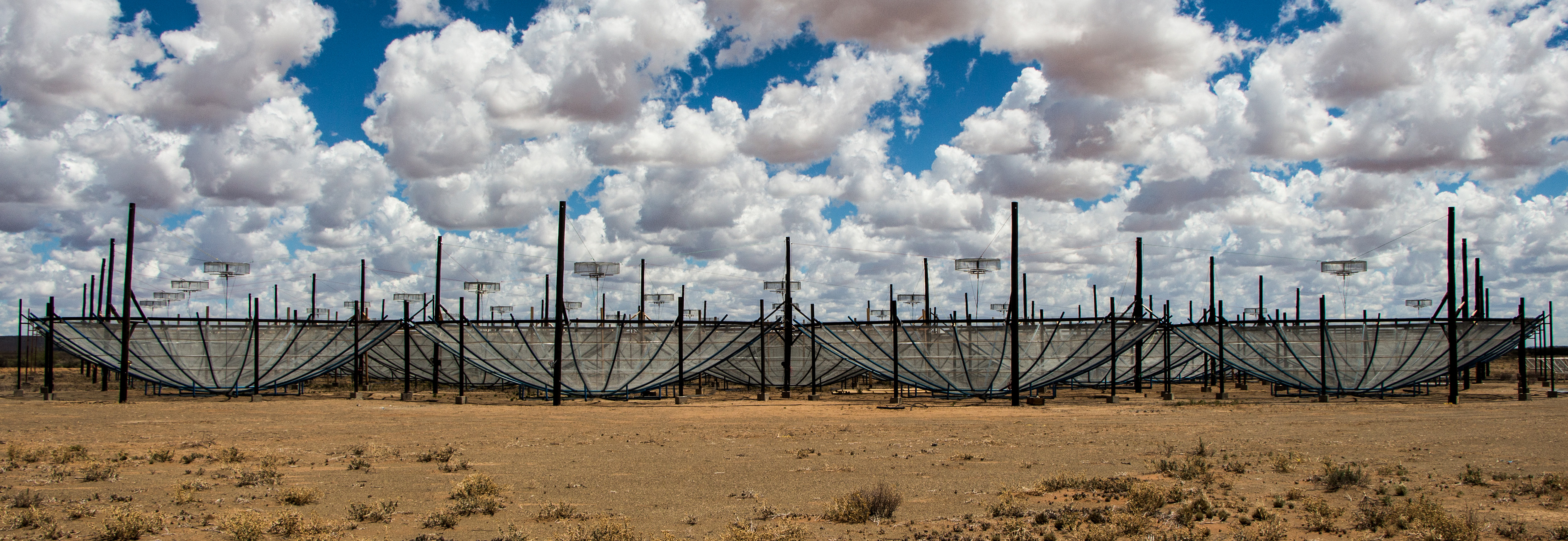
Figure 1: A view of HERA from January 2017. The data in this work were taken during Phase I, when HERA was composed of 14 m parabolic dishes with sleeved dipole feeds in mesh cages suspended at prime focus. These feeds were later replaced with wide-band Vivaldi feeds, expanding HERA’s bandwidth from 100–200 MHz (Phase I) to 50–250 MHz (Phase II).

During that time, the array continued to be built and commissioned. In Phase II, a new signal chain, correlator, and upgraded Vivaldi feeds have extended the bandwidth to 50–250 MHz (Fagnoni et al. 2020).

Recently, we reported the first upper limits on the 21 cm brightness temperature power spectrum from HERA in Abdurashidova et al. (2022a, hereafter H22a), using 18 nights of Phase I data and only 39 antennas. H22a built upon a number of supporting papers exploring various aspects of the data analysis. These included redundant-baseline calibration (Dillon et al. 2020), absolute calibration (Kern et al. 2020a), systematics mitigation (Kern et al. 2019, 2020b), error estimation (Tan et al. 2021), analysis pipeline architecture (La Plante et al. 2021), and end-to-end validation of that pipeline with realistic simulated data (Aguirre et al. 2022). We focused on the so-called “foreground-avoidance” approach to power spectrum estimation (Kerrigan et al. 2018; Morales et al. 2019), working predominately in foreground-free regions of Fourier space and applying conservative techniques that minimized potential signal loss or bias.

Our results, which constrained the “dimensionless” brightness temperature power spectrum to $\Delta^{2}(k)<$ 946 mK² at $z=7.9$ and $k=0.19$ $h$Mpc^-1 and to $\Delta^{2}(k)<$ 9,166 mK² at $z=10.4$ and $k=0.26$ $h$Mpc^-1 (both at the 95% confidence level), represented the most stringent constraints to date. They allowed us in Abdurashidova et al. (2022b, hereafter H22b) to constrain the astrophysics of reionization and the cosmic dawn and show that the IGM was heated above the adiabatic cooling limit by at least $z=7.9$. Evidence from other probes—including the integrated optical depth to reionization (Planck Collaboration 2018), observed galaxy UV luminosity functions, and quasar spectroscopy—indicates that reionization is likely well underway by $z=7.9$ (Mason et al. 2018; Greig et al. 2022). Our results therefore already rule out some of the most extreme of the so-called “cold reionization” models where an adiabatically cooling IGM produces a bright temperature contrast with the CMB, amplifying the 21 cm power spectrum as it is driven by ionization fluctuations (Mesinger et al. 2014).

In this work, we adapt and apply the analysis techniques of H22a and H22b to a full season of HERA Phase I data. Retaining the philosophy of foreground-avoidance and minimizing (and carefully accounting for) signal loss, we further tighten constraints on the 21 cm power spectrum at $z=7.9$ and $z=10.4$, and update the astrophysical implications of those limits. While some of our analysis techniques are updated to reflect an improved understanding of our instrument or adapted to better handle the larger volume of data considered, the core analysis techniques remain largely unchanged.

We begin in Section 2 by detailing the observations themselves and the basic cuts performed to ensure data quality. Then in Section 3 we review the data reduction steps performed to go from raw visibilities all the way to power spectra, highlighting updated analysis techniques and revised analysis choices. These techniques are tested with end-to-end pipeline simulations designed to validate our analysis choices and software in Section 4, in which we quantify a number of potential small biases and reproduce a few key figures from Aguirre et al. (2022) in the context of our new limits. In Section 5, we can then present our final power spectrum estimates, error bars, and upper limits. We build confidence in our results in Section 6 by applying a variety of statistical tests on our power spectra and how they integrate down across baselines and time. In Section 7, we report the impact of our new limits on the various approaches to astrophysical modeling and inference used in H22b, detailing our updated constraints on the epoch of reionization and the cosmic dawn. We conclude in Section 8, looking forward to potential future analyses of these data and data from the full HERA Phase II system.

2 Observations and Data Selection

In this work, we analyze observations with the HERA Phase I system that were performed over the period from September 29, 2017 (JD 2458026) through March 31, 2018 (JD 2458208). In Table 1, we summarize the key observational parameters of the instrument. For more detail about the precise configuration of the instrument, its signal chain components, and its FX correlator architecture, we refer the reader to DeBoer et al. (2017) and H22a. In this section, we discuss the process by which a selection of high-quality nights and antennas was performed.

Table 1: HERA Phase I observing and array specifications.

Array Location	$-$30.72∘S, 21.43∘E
Total Antennas Connected	47–71
Total Antennas Used	35–41
Shortest Baseline	14.6 m
Longest Unflagged Baseline	124.8 m
Minimum Frequency	100 MHz
Maximum Frequency	200 MHz
Channels	1024
Channel Width	97.66 kHz
Integration Time	10.7 s
Nightly Observing Duration	12 hours
Total Nights With Data	182
Total Nights Used	94

2.1 Selection of Nights and Epochs

Of the 182 nights during this season of simultaneous construction, commissioning, and observing, a significant fraction of nights was discarded for a variety of reasons. Most of these were hardware failures, including network outages, power outages, too many low- and/or high-power antennas, a briefly broadcasting antenna, broken receivers, and broken X-engines. Some were due to site issues, including high winds, a lightning storm, and excess radio frequency interference (RFI). While all nights have significant narrow-band RFI contamination from FM radio, TV broadcasts, and ORBCOMM satellites (see Section 3.2.3), most nights that were completely flagged for excess RFI showed consistent broadband emission contaminating channels typically free of RFI. These cuts first reduced the 182 nights to 104 nights using contemporaneous observing logs and real-time analysis. After inspecting hundreds of jupyter notebooks summarizing the nightly results of the data analysis pipeline after each key stage (see Section 3), this was reduced to 94 nights. For more details on the precise selection of nights, see Dillon (2021a).

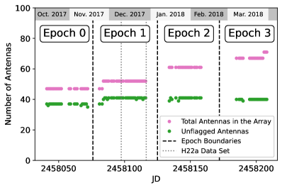
Figure 2: Here we show the observing season, split into epochs, and the number of antennas observing each night, both in total and after cuts. While the number of total antennas in the array grew from 47 to 71, the number passing all cuts remained roughly constant at $\sim$40. Epochs were defined by natural breaks in the observing season, mostly due to hardware issues. H22a analyzed data from 39 antennas on 18 nights, a subset of Epoch 1.

In Figure 2, we show how the nights passing our various data quality checks span the observing season. The breaks in good data (due to a network outage, a correlator malfunction, and a broadcasting antenna) naturally divided the season into four epochs. The data used in H22a were a subset of Epoch 1. While in theory each night could be analyzed independently before binning all of them together at constant local sidereal time (LST), we found it useful to analyze epochs individually, both for systematics mitigation (see Section 3.2.4) and for statistical tests on subsets of the data (see Section 6.3).

Because we observed during the Southern summer, most 12-hour “nights” included some data taken before sunset or after sunrise. These were flagged in our analysis. Further, a number of partial nights were flagged, usually due to excess RFI. The majority of these were due to broadband RFI during the first few hours of the night, possibly attributable to construction activity on site. A few other partial nights were flagged due to suspicious nightly calibration solutions, especially in Epoch 3 when the Galaxy was rising at the end of each night. More detail on the precise subset of nights flagged is given in Dillon (2021a).

The end result of our data cuts is a set of observations that, when LST-binned together, are significantly deeper than those in H22a, and cover over 21 hours of LST. As we can see in Figure 3, this data set peaks at $\sim$70 nights’ observing around 7 hours of LST, nearly four times deeper than the observations used in H22a.

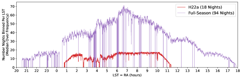
Figure 3: The full season of HERA data that we analyze spans nearly the full 24 hours of LSTs. Since we only observe at night, the time of greatest overlap in LST between nights occurs near the middle of the night in the middle of the season, at roughly 7 hours. At LSTs near that peak, this data set roughly quadruples the depth of the H22a data set. The increased number of flagged times (which cause vertical dips here) is due in large part to the changes in RFI excision (see Section 3.2.3).

Roughly speaking, this sets an upper bound on the factor by which our limits might improve due purely to the increase in sensitivity, since the noise on $P(k)$ scales inversely with observing time.

2.2 Selection of Antennas

Antenna selection began with the nightly data quality monitoring system described in H22a. It identified malfunctioning antennas by looking for antennas participating in baselines that were either outliers in total visibility power, or had visibility amplitude spectra significantly different from other baselines measuring the same physical separation on the ground. This procedure ultimately informed the most rigorous identification of malfunctioning antennas described in Storer et al. (2022), which was applied to HERA Phase II data. The results of nightly analysis were synthesized into a set of per-antenna, per-night flags by the HERA commissioning team as part of an internal data release.

Because our metrics for antenna quality are relative ones, we decided to expand and harmonize this list of flagged antenna-nights under the conservative presumption that antennas that misbehave consistently enough are probably also anomalous at some lower level on other nights. If, in any given epoch, an antenna was flagged more than 10% of the days, we flagged it for the whole epoch. If an antenna was completely flagged for more than 60% of the epochs that it appeared in (i.e. 3 of 4 epochs for antennas that were observing for the whole season), then it was completely removed.

Antennas passing this first series of cuts were then used for an initial round of redundant-baseline calibration where per-antenna gains and per-unique-baseline visbilities are solved for simultaneously as part of a large overdetermined system of equations (Liu et al. 2010). Antennas outside the southwest sector of HERA’s split-core configuration (155, 156, 180, 181, 182, and 183—see Figure 4—as well as two outriggers not pictured) were excluded as well because they would introduce extra tip-tilt degeneracies (Liu et al. 2010; Zheng et al. 2014, 2016; Dillon et al. 2018) and thus complicate a subsequent sky-based absolute calibration (Li et al. 2018; Kern et al. 2020a).

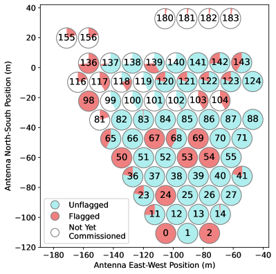
Figure 4: The layout of antennas during the season we analyze. Each antenna is a pie chart showing the fraction of the 94 total nights that each antenna was either flagged, unflagged, or not yet in the data set. The array was under construction as we observed, as can be seen by the northward expansion of the antennas available for observing. All antennas shown here numbered except 155, 156, and 180–183 would eventually become part of the southwest sector of HERA’s split-core configuration (Dillon & Parsons 2016; DeBoer et al. 2017).

As Dillon et al. (2020) describes, redundant-baseline calibration can be cast as a $\chi^{2}$-minimization problem where $\chi^{2}$ quantifies how consistent deviations from redundancy are with thermal noise (see Section 3.1 and Equation 2). If one attributes each baseline’s contribution to $\chi^{2}$ to both of its constituent antennas equally, one can form a $\chi^{2}$ per antenna statistic that is sensitive to particularly non-redundant antennas. In our first round of redundant-baseline calibration, antennas which made significant excess contributions to $\chi^{2}$ are flagged in 60-integration (i.e. 10.7 minute) chunks, and then calibration is performed again, iteratively, until no outliers remain. These were then likewise harmonized; antennas flagged for non-redundancy more than 20% of a night or 5% of an epoch were flagged for the whole night/epoch.

In Figure 4, we show the per-antenna flagging fraction after all of these cuts. The overall impact is that while the array was growing, the number of antennas included in our analysis remained largely static (see also Figure 2). Likely this set of nightly flags and antenna flags is overly conservative and some good data were thrown out. Due to the extreme dynamic range challenge faced by all of 21 cm cosmology, we adopted the stance that it was far safer to throw out possibly good data than to risk including bad data. Importantly, all these decisions about data selection were performed without reference to final power spectra and are therefore less likely to introduce experimenter bias. Once the set of good antennas-nights was selected, it was not subsequently changed.

3 Data Reduction and Systematics Mitigation

We now turn to a discussion of our data analysis pipeline, which we designed to reduce nightly visibilities to a final set of power spectra while avoiding systematics contamination. In general, our goal in this work is to apply the methods developed and validated in H22a and its supporting papers to this larger data set. This is a fundamentally iterative approach and likely does not leverage the full constraining power of the data set. Thus, the steps in the analysis pipeline—which we review in Section 3.1—remain largely unchanged.

However, a number of changes were incorporated in this work. Some were necessary because this data set is larger and more heterogeneous than the 18 nearly-contiguous nights examined in H22a with the same 39 antennas each night. Others are the result of various tweaks and minor improvements in the HERA team’s codebase developed between the H22a analysis and this work. Finally, some are simply minor changes in data analysis parameters and choices motivated by various intermediate data products. In Section 3.2 we report changes to our data reduction pipeline and in Section 3.3 we similarly detail changes to the estimation of power spectra and their errors and potential biases.

3.1 Overview of the Data Analysis Pipeline

H22a gives a detailed description of the analysis steps that take raw visibilities all the way to power spectra. Here we provide a high-level overview of each step in order to give context for the changes and updates in this analysis. We refer the reader to H22a and its supporting papers for more detail. The steps in our data reduction and systematics pipeline are as follows:

1. Redundant-baseline calibration: We begin with direction-independent calibration, wherein our observed visbilities, $V_{ij}^{\text{obs}}$, are modeled as

   $$V_{ij}^{\text{obs}}=g_{i}g_{j}^{*}V_{ij}^{\text{true}}+n_{ij}.$$ (1)

   Here $g_{i}$ is a complex, time- and frequency-dependent gain associated with the $i$th antenna and $n_{ij}$ is the noise on that visibility. Redundant-baseline calibration assumes that all baselines $\mathbf{b}_{ij}$ with the same physical separation and orientation should observe the same true visibility, and thus solves for both gains and unique visibilities as a large $\chi^{2}$-minimization problem, where

   $$\chi^{2}=\sum\limits_{i<j}\frac{\left|V_{ij}^{\text{obs}}-g_{i}g_{j}^{\ast}V_{i-j}^{\text{sol}}\right|^{2}}{\sigma_{ij}^{2}}.$$ (2)

   $V_{i-j}^{\text{sol}}$ here is the visibility solution for all redundant baselines with the same physical separation as $V_{ij}$. We calibrate by minimizing $\chi^{2}$ for every time and frequency independently, using only internal degrees of freedom and without reference to any model of the instrument or the sky. For an exploration of redundant-baseline calibration in the context of HERA, see Dillon et al. (2020).

2. Absolute calibration: The internal consistency of redundant baselines alone cannot solve for three important degrees of freedom, namely the overall gain amplitude and two phase tip/tilt terms. These degeneracies must be solved, per time and frequency, by reference to externally calibrated (or simulated) visibilities (Kern et al. 2020a). In H22a and in this work, we performed absolute calibration using a set of visibilities synthesized from three nights with LSTs spanning this data set (JDs 2458042, 2458116, and 2458207). These were calibrated on three separate fields using the MWA GLEAM catalog (Hurley-Walker et al. 2017) and CASA (McMullin et al. 2007), as described in Section 3.3 of H22a.

3. RFI flagging: RFI is identified and flagged using an iterative outlier detection algorithm described in H22a. Essentially, several sets of waterfalls (visibilities, gains solutions, etc.) are converted into time- and frequency-dependent measures of “outlierness” expressed as a $z$-score or modified $z$-score. This is done by looking at a 17$\times$17 pixel region centered on each pixel of the waterfall and measuring how consistent each it is with its neighbors in time and frequency. After averaging together $z$-scores of baselines or antennas to improve the signal-to-noise ratio (SNR), 5$\sigma$ outliers and 2$\sigma$ outliers neighboring 5$\sigma$ outliers are flagged. This is done independently for each set of waterfalls and the flags are then combined. We start RFI flagging with median filters and modified $z$-scores to reduce the effect of really bright RFI, then use those flags as a prior on a second round using mean filters and standard $z$-scores. Finally, we examine these statistics over the whole day, looking for whole channels or whole integrations that are 7$\sigma$ outliers and their 3$\sigma$ outlier neighbors. The same flags are applied to all baselines.

4. Gain smoothing: After flagging, all gains solutions are smoothed to mitigate the effect of noise and calibration errors, taking as a prior that the gains should be stable and relatively smooth in frequency. This smoothing is performed with a CLEAN-like deconvolution algorithm (Högbom 1974; Parsons & Backer 2009), filtering gains in 2D Fourier space on a 6 hour timescale and a 10 MHz frequency scale (or equivalently, 100 ns delay scale). These are the scales on which we have evidence for intrinsic gain variation in time (Dillon et al. 2020) and frequency (Kern et al. 2020a). For more implementation details, see H22a.

5. LST-binning: Having calibrated and flagged each night’s data, we then coherently average nights together on a fixed LST grid. This 21.4 s cadence grid—double the integration time of raw visibilities—is created by assigning each observation to the nearest gridded time and then rephasing that visibility to account for sky rotation due to the difference in LST. An additional round of flagging is performed on a per-LST, per-frequency, and per-baseline basis, looking for $5\sigma$ outliers in modified $z$-score among the list of rephased visibilities to be averaged together. This cut is designed to identify low-level residual RFI and calibration failures; it is highly unlikely to flag outliers due to noise.

6. Hand-flagging: After LST-binning, a final set of additional flags are added by manually examining high-pass delay-filtered residuals. This filtering was performed on using an iterative delay CLEAN to remove power below the 2000 ns scale in order to highlight spectrally compact features. Clear outlier channels and/or times that are consistent across baselines are flagged upon visual inspection. The same additional flags are applied to all baselines.

7. Inpainting flagged channels: When using Fast Fourier Transforms (FFTs) to form power spectra, flagged channels introduce discontinuities that leak foreground power to high delays. To avoid this, we use the same delay-based CLEAN algorithm to low-pass filter the data on 2000 ns scales and inpaint the flagged channels with the filtered result. Entirely flagged times are not inpainted. For more details and a demonstration of this procedure, see H22a.

8. Cable reflection calibration: When a signal bounces off of both ends of a cable before being transmitted, the result is a copy of the signal at a fixed delay associated with twice the light-travel time along the cable. Kern et al. (2020b) showed how the 20 m and 150 m cables in the signal chain produce these reflections, which can be represented as complex gain terms. While these gains are in principle calibratable with redundant-baseline calibration, our gain smoothing procedure completely removes them. Thus, following the procedure outlined in Kern et al. (2019), we iteratively model and calibrate out reflection and sub-reflection terms using autocorrelations, which have much higher SNR than cross-correlations. Since cable reflections are stable over many nights, this is done after LST-binning.

9. Crosstalk subtraction: Kern et al. (2020b) also demonstrated the pernicious impact of crosstalk systematics across a large range of delay modes in HERA Phase I data. It was hypothesized that this was due to over-the-air crosstalk that led to autocorrelations leaking to cross-correlations at high delays. In Appendix A, we show how this effect’s delay and amplitude structure can be explained by an emitter in the signal chain. Because autocorrelations are non-fringing and thus quite stable in time, the effect can be mitigated by modeling each baseline’s excess power near zero fringe-rate. Kern et al. (2019) does this using singular value decomposition (SVD) to find the delay and time modes affected and uses Gaussian process regression to limit the range of fringe-rates modeled and subtracted so as to avoid EoR signal loss. That fringe-rate range is symmetric about zero and limited by the east-west projected baseline length $|b_{\text{E-W}}|$ such that

   $$\left|f_{\text{max}}\right|=0.024\text{\,mHz}\left(\frac{|b_{\text{E-W}}|}{1\text{\,m}}\right)-0.28\text{\,mHz}.$$ (3)

   The signal loss due to crosstalk subtraction was calculated in Aguirre et al. (2022) and corrected for in H22a; we repeat the calculation in Section 4.3 and find similar results. Crosstalk subtraction is not applied to baselines with projected east-west distances less than 14 m, since the zero fringe-rate mode overlaps with the fringe-rates associated with the main lobe of the primary beam (Parsons et al. 2016).

10. Coherent time averaging: Following H22a, we next coherently average visibilities from the 21.4 s cadence after LST-binning down to a 214 s cadence, using the same rephasing procedure described above to account for sky-rotation. This timescale was chosen to keep signal loss at the $\sim$1% level (Aguirre et al. 2022); we repeat that calculation for this data set in Section 4.3 and find consistent results.

11. Forming pseudo-Stokes I visibilities: Before forming power spectra, we construct pseudo-Stokes visibilities. As H22a showed, this limits the leakage of Faraday-rotated foregrounds into high-delays, though $Q\rightarrow I$ leakage from primary beam asymmetry is still possible (Moore et al. 2013; Asad et al. 2016; Kohn et al. 2016; Nunhokee et al. 2017; Asad et al. 2018). For the pseudo-$I$ channel, this step consists of simply averaging together the $EE$- and $NN$-polarized visibilities for the same baseline, where $E$ and $N$ denote the east- and north-aligned linearly-polarized feeds respectively (Kohn et al. 2019).

12. Power spectrum estimation: We compute power spectra using the delay approximation, in which we substitute a Fourier transform along the frequency axis of a visibility (i.e. a delay transform) for a line-of-sight Fourier transform (Parsons et al. 2012a). This strategy avoids mapmaking entirely (Dillon et al. 2013, 2015b; Xu et al. 2022). We thus approximate $\tau$ and $u$ (the magnitude of the baseline in units of wavelengths) as mapping linearly to line-of-sight Fourier modes, $k_{\|}$, and transverse Fourier modes, $k_{\perp}$, respectively. The power spectra are estimated by taking the real part of

    $$\hat{P}(k_{\perp},k_{\parallel})=\frac{X^{2}Y}{\Omega_{pp}B}\widetilde{V}_{\text{1}}(u,\tau)\widetilde{V}_{\text{2}}^{\ast}(u,\tau),$$ (4)

    where $\widetilde{V}$ is a Fourier transformed visibility in frequency. $\Omega_{pp}$ is the full-sky integral of the squared primary beam response—we use the beam simulated in Fagnoni et al. (2021)—and $B$ is the bandwidth. $X$ and $Y$ are scalars mapping angles and frequency to cosmological distances, defined via $k_{\|}=2\pi\tau/X$, $k_{\perp}=2\pi|\mathbf{b}|/(Y\lambda)$, with $X=D(z)$ and $Y=c(1+z)^{2}[H(z)]^{-1}/(1420\text{\,MHz})$, where $H(z)$ is the Hubble parameter, and $D(z)$ is the transverse comoving distance (Hogg 1999). $\hat{P}(k_{\perp},k_{\parallel})$ here is in units of ${\rm mK^{2}}\ h^{-3}\ {\rm Mpc^{3}}$, though it conventional to report the “dimensionless” power spectrum (which has units of ${\rm mK^{2}}$):

    $$\Delta^{2}(k)\equiv P(k)\frac{k^{3}}{2\pi^{2}}.$$ (5)

    H22a shows how this can be recast into the language of quadratic estimators (Tegmark 1997; Liu & Tegmark 2011; Dillon et al. 2013; Trott et al. 2016). In that formalism, we use a diagonal normalization matrix $\mathbf{M}$ (i.e no decorrelation of bandpower uncertainties). In lieu of any inverse covariance weighting, we use a Blackman-Harris taper to prevent foreground leakage into the EoR window. When computing Equation 4, we cross-multiply Fourier transformed visibilities from alternating 214 s blocks of time (i.e. $\widetilde{V}_{1}$ and $\widetilde{V}_{2}$), using all pairs of baselines in a redundant baseline group. In the (quite accurate) approximation that visibilities interleaved in this way have uncorrelated noise, this produces an estimate of the power spectrum free of noise bias.

13. Error estimation: As in H22a, we employ the noise estimation formalism of Tan et al. (2021). The noise power spectrum is given by

    $$P_{N}=\frac{X^{2}Y\Omega_{\rm eff}T^{2}_{\rm sys}}{t_{\rm int}N_{\rm coherent}\sqrt{2N_{\rm incoherent}}},$$ (6)

    where $T_{\rm sys}$ is the system temperature, $t_{\rm int}$ is the integration time, and $N_{\rm coherent}$ and $N_{\rm incoherent}$ are the numbers of integrations averaged together coherently or incoherently—i.e. averaged as visibilities with phase information or averaged as power spectra. $\Omega_{\rm eff}$ is the effective beam area, defined as $\Omega_{\rm eff}\equiv\Omega_{p}^{2}/\Omega_{pp}$ in Appendix B of Parsons et al. (2014). We use the inverse square of the noise power spectrum to perform inverse variance-weighted averaging of the power spectra. For reporting final errorbars on power spectra, we use an unbiased estimator of the noise and signal-noise cross-terms developed by Tan et al. (2021),

    $$\hat{P}_{\rm SN}=P_{N} \left(\sqrt{\sqrt{2}(\hat{P}/P_{N})+1}\right.$$

    $$\left.~{}\left[\sqrt{1/\sqrt{\pi}+1}-1\right]\right).$$ (7)

14. Incoherent power spectrum averaging: Here and in H22a, power spectra are averaged incoherently over several axes to produce the final limits. First, all baseline-pairs within a redundant baseline group are averaged, ignoring auto-baseline pairs (power spectra formed from the same pair of antennas at interleaved times). This preserves most of the sensitivity of coherently averaging visibilities within a redundant group before forming power spectra, while excluding the pairs most likely to exhibit correlated systematics. Then power spectra are averaged incoherently in several disjoint LST ranges, which we call “fields” since they correspond to different parts of the sky at zenith. Power spectra are estimated independently for the LST ranges in the separate fields and we perform no further averaging in H22a or this analysis when reporting power spectrum upper limits. Finally, we perform a binning to spherical $k=\sqrt{k_{\|}^{2}+k_{\perp}^{2}}$, excising baselines based on their length and certain sets of delay modes based on their proximity to the “horizon wedge,” which is set by the light travel time along the baseline

    $$\tau_{\text{wedge}}=|\mathbf{b}|/c.$$ (8)

    $P_{N}$ and $\hat{P}_{\rm SN}$ are propagated through each of these averaging steps.

For more details on the implementation of these techniques, we refer the interested reader to H22a and its supporting papers.

3.2 Updates to the Data Reduction and Systematics Mitigation Pipeline Since H22a

With the full context of the analysis pipeline established above, we now detail the ways it has changed since H22a. While most are relatively minor tweaks (Dillon 2021a), we detail them here for completeness and reproducibility.

3.2.1 Updates to Redundant-Baseline Calibration

Two minor changes were made to redundant-baseline calibration. The first is the addition of a step in firstcal—the solver for per-antenna delays and phase offsets (Dillon et al. 2020)—to also solve per-antenna polarity flips. A polarity flip, which could result from rotating the feed by 180^∘, simply flips the sign on the measured voltage from the antenna or equivalently multiplies the gain by $-1$. Solving for polarities allows firstcal to converge faster and more reliably, but does not appreciably change the result.

The second change was an increase of the maximum number of iterations allowed in omnical, which uses damped fixed-point iteration to minimize $\chi^{2}$ in Equation 2 (Dillon et al. 2020). This was increased from 500 to 10,000. This likely makes little difference in practice, since omnical usually only converges that slowly for a given time and frequency in the presence of bright RFI contamination. Since allowing more steps did not substantially increase runtime (individual times and frequencies can converge independently), we felt it was safer give the algorithm as long as necessary to minimize $\chi^{2}$, even if doing so had little impact after gain smoothing.

3.2.2 Updates to Absolute Calibration

Two important changes were made to absolute calibration as compared to H22a. The first is a change to how flags are propagated from the sky-calibrated reference visibilities. Previously, antennas flagged or otherwise not included in the reference set of visibilities were also flagged on a nightly basis after absolute calibration. In this work, these antennas are simply given zero weight when solving for the degeneracies of redundant-baseline calibration—which are then applied to all gain solutions. Per-antenna flags, once set (see Section 2.2), did not change during the nightly calibration.

Second, we added a new step in absolute calibration to fix the bias discovered in the course of validating the H22a pipeline. In Aguirre et al. (2022), we found that absolute calibration produced gains that were biased high and that the bias got larger with decreasing visibility SNR. This is particularly worrisome because gains affect both power spectrum and error estimates quartically, and high gains lead to artificially low power spectrum estimates. In Aguirre et al. (2022) we calculated the size of this effect and in H22a we increased our measurements and error bars to compensate for this $\sim$10% bias on our power spectra.

A detailed mathematical account of the origin of the bias appears in Appendix B of Byrne et al. (2021). However, it can be understood intuitively as follows: when solving for the overall gain degree of freedom in absolute calibration, noise turns individual visibilities in the complex plane into samples of a circularly symmetric distribution whose center is displaced from the origin (the “true” visibility). When measuring magnitudes, that probability distribution is Ricean and always has a larger mean than the magnitude of the “true” visibility. Simply put, adding symmetric noise is more likely to increase the amplitude of a complex number than decrease it. However, by calibrating the overall multiplicative amplitude as a complex number and then only taking the absolute value at the very end, one can avoid this bias—as we show in Section 4.2 and Figure 13.

3.2.3 Updates to RFI Excision

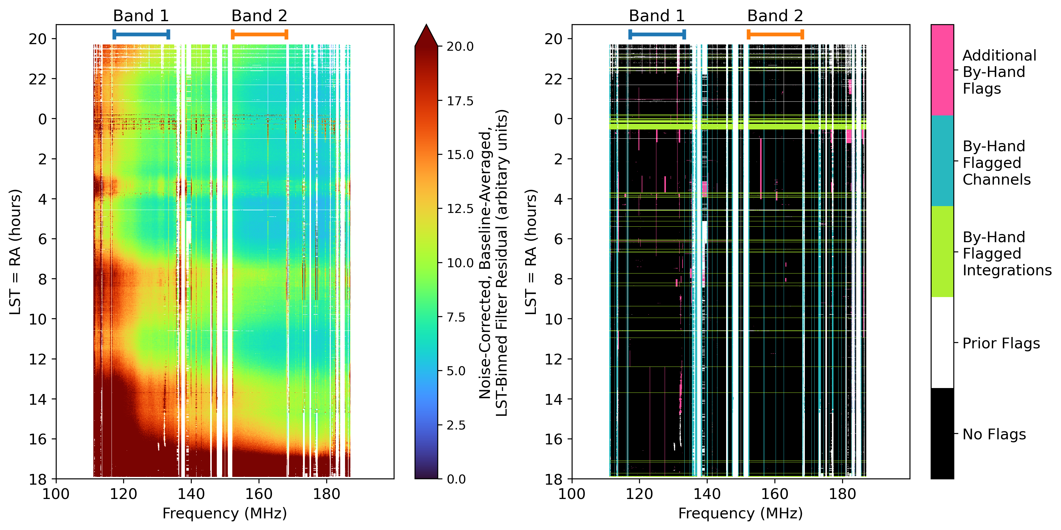
Figure 5: Here we illustrate the process for RFI excision after binning together all 94 days. On the left, we show 2000 ns high-pass filter residuals of all epochs combined. It shows some clear temporal and spectra structure which necessitates further flagging. These additional flags, shown on the right, are performed first by looking for outlier channels or integrations, then by hand-flagging contiguous regions of excess structure. We attribute these outliers to low-level RFI, as well as the interplay between the night-to-night variation in the RFI flagging mask and night-to-night changes in calibration errors. Most of the additional flagged pixels in this waterfall were already flagged on a significant fraction of the nights.

While the fundamental algorithm for RFI excision remains unchanged, we made two updates to how it was performed on a nightly basis. The first is related to how the analysis dealt with data file boundaries. Previously, every data file was analyzed in parallel for RFI. Since the outlier identification algorithm relies on neighboring times and frequencies, this became less reliable near file boundaries where there are roughly half as many neighbors to compare to, and likely led to some of the $\sim$10 minute periodicity we saw in the flags in H22a. In this analysis, we parallelized the pipeline in overlapping time chunks, so that every point was compared to exactly the same number of neighbors—except at the beginning and end of the night and at the edges of the band.

Second, we modified the set of data products used in searching for outliers. In both analyses we used raw visibilities (albeit only in the mean filter round); gains from both redundant-baseline calibration and absolute calibration; and $\chi^{2}$ from both calibration steps. Based on experiments we performed on which data products were providing unique information and not leading to overflagging, we removed a global cut on outliers in $\chi^{2}$—which likely led to the over-flagging around Fornax A in H22a—and added uncalibrated autocorrelations for their high SNR and computational tractability compared to the full set of visibilities. The result is still a very expansive set of flags and likely contains a significant number of false positive identifications of RFI, especially around ORBCOMM at 137 MHz and the clock line at 150 MHz (see e.g. Figure 5 and Figure 8). Given the extreme dynamic range requirements of 21 cm cosmology, it is far safer to over-flag than under-flag (Kerrigan et al. 2019).

In that spirit, we also revisited how a final set of by-hand flags were identified. In H22a, this flagging was performed by examining a handful of key baselines after high-pass filtering to remove structure below the 2000 ns scale. In this work, the four epochs were first combined together without any inpainting, reflection calibration, or crosstalk subtraction. After performing the same per-baseline high-pass filter on every baseline, their amplitudes were averaged together, inverse variance weighted by noise and then corrected for the noise bias.

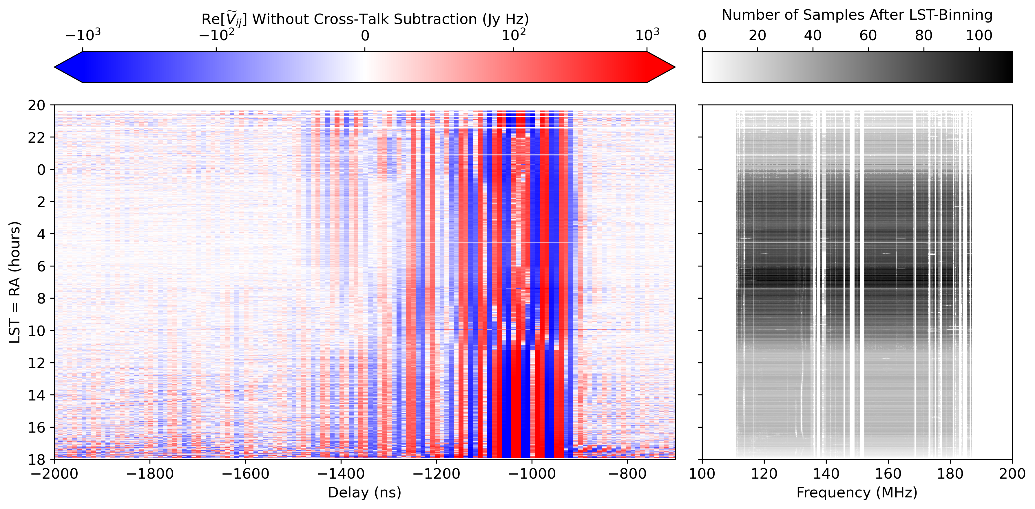
Figure 6: In Kern et al. (2020b), the observation that the phase of crosstalk systematics remained stable in delay in space was key to removing them down to nearly the noise level. This technique proved foundational to our results in H22a. However, when we combined all four epochs together, we began to see discontinuities in the phase structure of the crosstalk. In the left panel, this effect is particularly clearly illustrated in Band 1 of the north-polarized baseline between antennas 11 and 66. We see a number of delay modes where the sign of the crosstalk feature abruptly shifts from positive to negative (or vice versa) as a function of LST. These discontinuities appear to be associated with epoch boundaries, which give rise to discontinuities in the number of samples binned together (right panel). We hypothesize that these discontinuities arise due to the effects of the ongoing construction of HERA, either on the source of the crosstalk emission or on how it is transmitted through the array (see Appendix A for more detail).

The result, shown in the left-hand panel of Figure 5, highlights residual frequency structure. Much of this has low $N_{\text{samples}}$ and/or borders on previously identified RFI, indicating its origin as low-level, inconsistently flagged RFI. As the right-hand panel shows, outlier channels and integrations were first identified by averaging along each axis. Next, individual areas of concern were flagged by hand, by converting the waterfall to a bitmap image and individually marking times and frequencies in Adobe Photoshop. An effort was made to flag coherent rectangular regions near previously identified flags to avoid cherry-picking, though fundamentally this step involved a series of subjective judgment calls. Once the final flagging waterfall was developed, it was not revisited after estimating power spectra in order to avoid experimenter bias.

3.2.4 Updates to Reflection Systematics and Crosstalk Mitigation

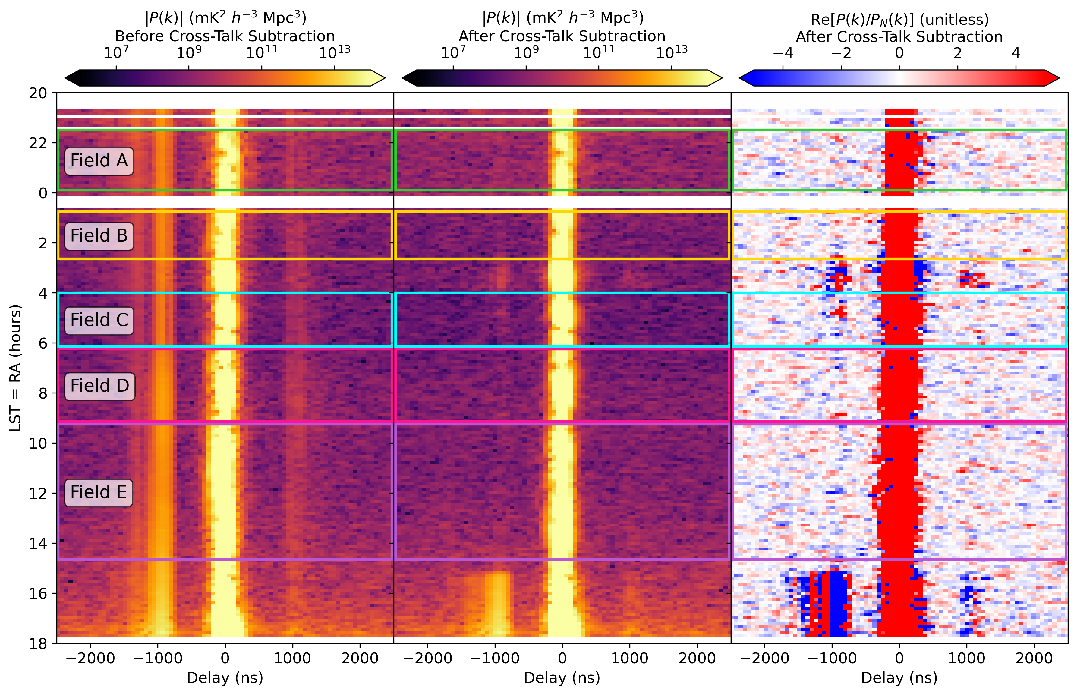
Figure 7: Here we show the effect of our crosstalk subtraction algorithm on the power spectrum of a baseline-pair (in this case, 38–66 crossed with 52–82 in Band 1) with a particularly strong crosstalk signal at negative delay. The technique of Kern et al. (2019), applied on a per-epoch basis, removes the crosstalk features seen here at roughly $\pm$1000 ns down to a level nearly consistent with noise even after averaging all four epochs together. Since the crosstalk is proportional to the amplitude of the autocorrelations (see Appendix A), which rise very steeply when the Galactic center transits the beam at 17.8 hours LST, and since our removal algorithm depends on the temporal stability of the crosstalk, we give LSTs between $\sim$15.3 and 21 hours zero weight. This results in cleaner residuals in the more sensitive fields, at the price of greater residuals at high LST. This also motivated our definition of the five fields in which the power spectrum was independently estimated; see Section 3.3.1 and Figure 9 for more details on the definition of the fields.

In H22a, all the steps in Section 3.1 after LST-binning were performed on the full-sensitivity, 18-night data set. At first, we attempted performing the same analysis with all 94 nights binned together but found that the level of residual crosstalk had substantially higher SNR than anything seen in H22a. Some baselines were particularly bad, exhibiting a delay- and time-averaged SNR greater than 10 in the affected delay range. Upon examining the pre-subtraction waterfalls of the baselines where crosstalk subtraction performed the worst, we found clear evidence for temporal structure in the delays contaminated by crosstalk. In Figure 6, we show one such baseline. Plotting the real part of its waterfall in delay space shows clear temporal structure at certain delays, including some where it flips from positive to negative and vice versa. This is potentially disastrous for the crosstalk subtraction technique of Kern et al. (2019), which relies on stability in delay space.

Furthermore, there appears to be a correlation between discontinuities in $N_{\text{samples}}$ (right-hand panel of Figure 6) and discontinuities in the delay structure of $\tilde{V}_{ij}$. Since the former are largely attributable to epoch boundaries, which affect how often each LST is observed, we hypothesized that the changing and growing array was affecting the precise structure of the crosstalk. This ultimately pointed us toward a new understanding of the physical origin of the effect, namely that all antennas’ signals were being broadcast from one point on the west side of the array, likely the refrigerated enclosures which contained the analog receivers. We discuss this model and the evidence for it in detail in Appendix A.

The upshot of this result is twofold. First, it confirms that the model of Kern et al. (2019), of autocorrelations leaking into cross-correlations, is correct. Second, it implies that as long as the array is stable, the effect should be stable in LST-binned data as well. We therefore decided to perform inpainting, cable reflection calibration, and crosstalk subtraction on a per-epoch basis before binning together the four epochs. This proved a substantially better approach—as Figure 7 shows—and got us much closer to consistency with noise after crosstalk subtraction.

A few minor tweaks were also made to cable reflection calibration and crosstalk subtraction. The total number of terms used to fit the cable reflections was increased from 28 terms between 75 and 1500 ns to 35 terms between 75 and 2500 ns, to both better model the 20 m cables and to be able to model a few extra long cables whose reflection timescale were larger than 1500 ns but were not in the H22a data set. The SVD used in crosstalk subtraction was previously limited to 30 delay modes; we increased it to 50 based on experiments where it made the crosstalk residuals a bit more consistent with noise. Finally, we revised how weights were applied before computing the SVD. First, we weighted each time by the frequency-averaged number of samples. H22a used an unweighted SVD, but as Figure 3 shows, the approximation of weights that are constant in time breaks down when considering such a large and discontinuous data set. Second, we also set the weight in the SVD to zero from 15.3–21 hours to prevent bright galactic emission at the edge of the data set from introducing temporal structure that caused the crosstalk subtraction procedure to perform worse for the most sensitively measured LSTs.

3.3 Updates to Power Spectrum Estimation Since H22a

Just as with the data reduction pipeline, we sought to apply the same power spectrum analysis procedures and choices as were used in H22a. However, differences in LSTs observed, flagging, and systematics removal motivated slightly different approaches to how the data should be reduced and cut. These decisions were made without reference to the final power spectra in order to minimize experimenter bias.

3.3.1 Picking Bands and Fields

The two frequency bands analyzed in H22a were Blackman-Harris tapered ranges from 117.09–132.62 MHz and 150.29–167.77 MHz. These were motivated by the two contiguous regions of low flag occupancy (see Figure 12 in H22a). We reproduce that same plot in Figure 8 and following the same logic—albeit with somewhat different flags—pick Band 1 and Band 2 to range from 117.19–133.11 MHz and 152.25–167.97 MHz, respectively. The bands still center on approximately the same redshifts: $z=10.4$ and $z=7.9$.

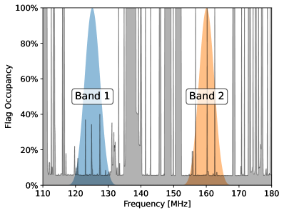
Figure 8: The two frequency bands used in this analysis were chosen to avoid sections of the band with heavy flagging. Here we illustrate the bands as Blackman-Harris windows, indicating the relative weight of the different channels in our final power spectra. These two bands are from 117.19–133.11 MHz and 152.25–167.97 MHz, corresponding to $z=10.4$ and $z=7.9$ respectively. These bands differ very slightly from the bands with the same names used in H22a.

Because we observed a larger range of LSTs than in H22a, we need to define new fields (i.e. new LST ranges) in which to independently estimate power spectra. In order to motivate the choice of fields without reference the final power spectra, we looked at two other statistics, which we plot in Figure 9.

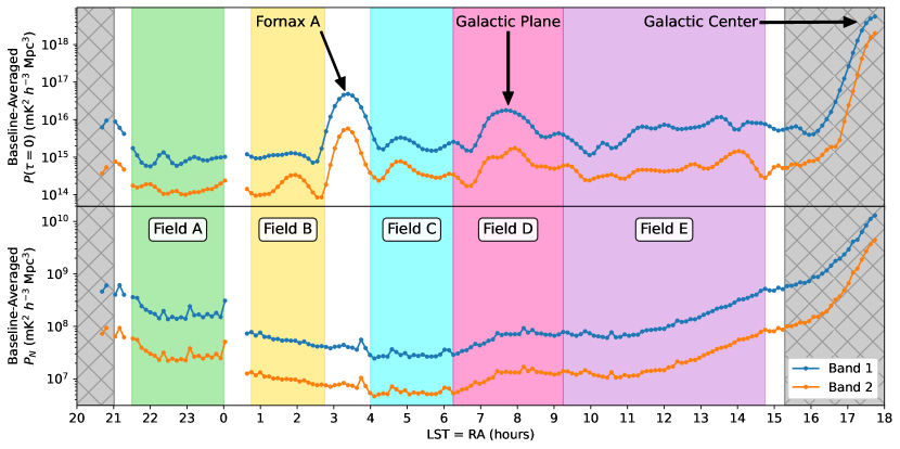
Figure 9: Two metrics—the baseline-averaged power spectrum at $\tau=0$ in the top panel, and noise power spectrum amplitude in the bottom panel—were used to divide the data set into fields in which to independently estimate the power spectrum. Following H22a, which divided the data set into three fields, we divide the data set into five and label them A, B, C, D, and E since they do not directly correspond to the fields used in H22a. As we describe in Section 3.3.1, we picked the fields to avoid gaps in the data, Fornax A (at 3.4 hours), and the galactic center (at 17.8 hours). These are all features that introduce sharp temporal changes that make crosstalk subtraction more difficult. We also wanted to avoid the times where the SVD in the crosstalk subtraction was given zero weight (gray hatched region) to avoid affecting the more sensitive fields.

These two statistics are the inverse-variance-weighted, baseline-averaged delay-zero power, $P(\tau=0)$—a proxy for foreground power—and $P_{N}$, which is flat in delay and tells us about both foreground power and total observation time. We used these to define a total of five fields: A (21.5–0.0 hours), B (0.75–2.75 hours), C (4.0–6.25 hours), D (6.25–9.25 hours), and E (9.25–14.75 hours). We restricted our field boundaries to quarter-hour increments to avoid cherry-picking integrations.

The rationale for defining the fields is as follows. We wanted fields B, C, and D, to correspond reasonably well to fields 1, 2, and 3 in H22a, so to cover the new LST ranges, we added fields A and E. Field A was set by the flagging gaps at either end, intentionally avoiding the last integration before the flagging gap between 0 and 1 hours due to the potential for signal loss from crosstalk subtraction (Aguirre et al. 2022). Likewise, field B was defined to exclude the first integration after the gap and keep Fornax A in the main lobe no brighter than its brightest point in the first sidelobe around 2 hours. Field C was defined to start at a roughly symmetrical place to where Field B ended with respect to Fornax A and to include the range of maximum sensitivity from roughly 4–6 hrs. Thus, the upper field boundary was set by the sidelobe of the Galactic plane at 6.25 hours. The boundary between fields D and E was set to include the roughly symmetrical sidelobe at $\sim$9 hours within Field D, keeping the Galactic plane contained to a single field. Field E ends a bit before where the cross-talk subtraction gets zero weight in the SVD. Once these field definitions were established, they were not allowed to change.

3.3.2 Excluding Baseline Pairs with Substantial Residual Crosstalk

Despite subtracting crosstalk on a per-epoch basis, we still found strong evidence for residual crosstalk on certain baselines. In the baseline examined in Figure 7, we can see clear residual power as an excess SNR in the delay range of $800<|\tau|<1500$ ns (right-hand panel). This is most prominent near the Galactic center, which got zero weight in the SVD, and near Fornax A, but there appears to be a slight excess at other LSTs as well. To quantify this, we averaged $|$SNR$|$ over that delay range and over the three most sensitive fields, B, C, and D. This average was performed separately for positive and negative delays, since we now know that those two signals have independent origin (see Appendix A).

We computed this averaged $|$SNR$|$ for every auto-baseline pair (i.e. power spectra formed from the same baseline at interleaved times, rather than power spectra formed from different but redundant baselines) and plotted a histogram of it for each band in Figure 10, treating positive and negative delays as independent samples.

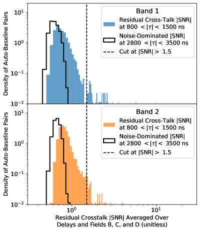
Figure 10: While our crosstalk subtraction algorithm removes the vast majority of the systematic, the technique is not perfect. We quantify the level of residual crosstalk by taking the average magnitude of the SNR in our most sensitive fields—B, C and D—and in the delay range most affected by crosstalk, $800<|\tau|<1500$ ns. Comparing this quantity to the same quantity computed in the noise-dominated delay-range of $2800<|\tau|<3500$ ns, we find significant excess. Using auto-baseline-pairs, which are not included in the final power spectrum, we eliminate baselines with $|$SNR$|>1.5$. Note that our most sensitive upper limits come from lower delays, so this is not a potentially biasing cut on SNR in the final quantity of astrophysical interest. Because the cross-talk at positive and negative delay is sourced independently (see Appendix A), we perform this cut separately for positive and negative delays. Because, by convention baselines are east-west-orientated and not west-east-oriented and because the crosstalk emitter is close to the west side of the array, more negative delays are flagged than positive delays. In all, this cut flags 3.5% and 3.8% of baselines at negative delays for bands 1 and 2, respectively, and 1.0% and 0.9% of baselines at positive delays.

Compared to an equivalently sized delay range from $2800<|\tau|<3500$ ns (solid black), we see evidence for a mild excess on most baselines. This is perhaps not too surprising; the crosstalk subtraction algorithm of Kern et al. (2019) attempts to model and subtract the crosstalk down to the noise—in our case, the noise in a single epoch. To the extent that crosstalk remains correlated from epoch to epoch, integrating down should reveal more crosstalk. That said, there is a tail of outliers in Figure 10 that motivated us to perform a cut at $|$SNR$|>1.5$. The cut was performed separately for positive and negative delays, so some baseline pairs are “half-flagged.” The vast majority of auto-baseline pairs ($>$95%) were kept. More baseline-pairs were cut at negative delays than positive delays because the antenna ordering means that negative delays were more often associated with antennas nearer the crosstalk source (see Appendix A).

We also computed the $|$SNR$|$ for cross-baseline pairs as well and found that they were highly correlated with the $|$SNR$|$ of the two corresponding auto-baseline pairs. However, we decided to more conservatively use only the auto-baseline pairs—which are not included in the final power spectra—for our cut. Any cross-baseline pair with one baseline participating in a flagged auto-baseline pair (and delay sign) was flagged. This cut is the most surgical and perhaps more worrisome analysis change from H22a, in the terms of removing individual power spectra before averaging. However, by only looking at high $|\tau|$—well above the corresponding $k$ values where we set our tightest upper limits—and by using only the auto-baseline-pairs, we insulate ourselves from the risk of cherry-picking and signal loss.

One other key change from H22a is the shortest east-west projected baseline length allowed to be included in our final spherical power spectra. Even after averaging cross-baseline pairs within redundant groups, we still see a substantial uptick in $|$SNR$|$ in the crosstalk delay range for baselines with 14.6 m projected east-west baselines, the shortest baselines used in H22a (see Figure 11).

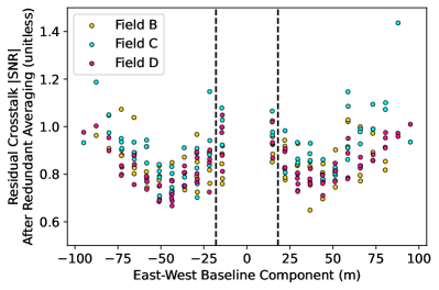
Figure 11: Even after flagging baselines for residual crosstalk, averaging the power spectra of cross-baseline pairs incoherently within redundant groups shows residual crosstalk. This is not surprising, since Figure 10 showed ubiquitous excess in this delay range. What averaging reveals more clearly is an important trend in crosstalk $|$SNR$|$ with projected east-west baseline. Baselines with small east-west components are the slowest fringing, which means that the crosstalk subtraction algorithm of Kern et al. (2019) only attempts to remove crosstalk in a relatively small range of fringe rates for fear of removing cosmological signal. That is why baselines with east-west components less than $14$ m were removed before power spectrum estimation in H22a and do not appear here either. Based on this metric, we decided to extend that cut to baselines with east-west components less than 15 m (those inside the dashed lines), which includes all single-unit separated baselines in the hexagonal grid (see Figure 4). While some other long baselines also show strong residuals, this noted jump among the most sensitive baselines was concerning enough to merit a cut.

This makes sense physically—these baselines have their main lobe closest to zero fringe-rate, where the crosstalk subtraction algorithm only operates on a very narrow range of fringe-rates (Equation 3) for fear of signal loss. While the crosstalk is centered at 0 mHz, it has some width in fringe-rate space. We expect, therefore, that these baselines should be the first to show residual cross-talk as we integrate down. It was also likely true in H22a; the lower noise level in these data simply makes the systematics clearer.

We decided to conservatively increase that cut to 15 m, throwing out several redundant baseline groups, including the most sensitive single baseline group used in H22a, the single-unit 14.6 m east-west baseline. To keep this baseline without simply accepting excess systematics, we would have had to find a way to more aggressively filter crosstalk, which would then have necessitated a more thorough and precise quantification of baseline-dependent signal loss using end-to-end simulations. Since our aim in this work is to apply the analysis of H22a as directly as possible, we defer such an investigation to future work.

3.3.3 Changes to $k$ Cuts and Bins

The final key analysis change between H22a and this work is an increase in the area of power spectrum modes that were excised from within the EoR window (but still near the wedge). In H22a, the modes excluded from the spherical power spectra were all those within 200 ns of the horizon wedge (Equation 8). This “wedge buffer” has a long history in the field, going back to Parsons et al. (2012a), which suggested that a combination of foreground and beam chromaticity and the application of tapering functions in the delay power spectrum can extend power $\sim$0.15 $h$Mpc^-1 beyond the horizon wedge. The choice of 200 ns in H22a (equivalent to 0.11 $h$Mpc^-1 at $z=7.9$ and 0.10 $h$Mpc^-1 at $z=10.4$) was motivated by Figures 14 and 15 of that paper, which show power spectrum SNRs after cylindrically binning to $k_{\|}$-$k_{\perp}$ space. The buffer was picked to mostly exclude the region of $k$-space with SNR consistently larger than 1, while balancing that exclusion of foreground-dominated modes at low $k_{\perp}$ against the admission of noise-dominated modes at high $k_{\perp}$.

Reassessing the same question in light of our equivalent plots of SNR in cylindrical $k$-space (Figure 17 and Figure 18), we increase the wedge buffer to 300 ns, to achieve roughly the same balance of excluding and admitting modes. We picked 300 ns as a round number to avoid cherry-picking. This produces a wedge buffer at $k=0.15$ $h$Mpc^-1 in Band 1 and $k=0.17$ $h$Mpc^-1 in Band 2, which is more in line with the value suggested by Parsons et al. (2012a), and used in early HERA forecasts (Pober et al. 2014). That said, increasing the wedge buffer is another sensitivity hit, so finding other ways to mitigate foreground emission near the wedge (e.g. Ewall-Wice et al. 2021) in future work might increase the constraining power of this data set.

One other minor change to our spherical power spectra is our precise binning in $k$. In most of the EoR window, $k$ is dominated by $k_{\|}$, which maps to $\tau$. H22a picked $k$ bin centers and widths with the intention that two $\tau$ modes would fall into each bin. However, using a fixed $\Delta k$ of 0.064 $h$Mpc^-1 for both bands, with the first bin centered at $k=0$, did not quite achieve this. Some fixed-$\tau$ modes got split between $k$ bins and some $k$ bins had more power spectra averaged together than others. To achieve a better alignment with $k$ bin centers nearer the average $k$ value of modes in the bin, we used $\Delta k=0.0619$ $h$Mpc^-1 in Band 1 and $\Delta k=0.0709$ $h$Mpc^-1 in Band 2m with the first bin centered at $3\Delta k/4$. For more details on this change, see Dillon (2021b).

3.3.4 More Precisely Calculating Power Spectrum Window Functions

The expectation value of the estimated power spectrum for a given baseline and delay, $\hat{P}(\mathbf{u},\tau)$, is actually a weighted sum of the neighboring true bandpowers $P(\mathbf{k})$. These weights are usually referred to as the window functions $W$, defined through

$$\hat{P}(u,\tau)\propto\int\mathrm{d}^{3}\mathbf{k}\,P(\mathbf{k})\,W(\mathbf{k};\mathbf{u},\tau).$$ (9)

In H22a, the horizontal error bars on the spherical power spectrum were evaluated with the same assumptions made to analyze the data, i.e. the delay approximation, in which the delays and line-of-sight Fourier modes are treated interchangeably. This leads to underestimating the tails of the window functions, and in particular the foreground power leaking into the EoR window at low $k_{\parallel}$ (Liu et al. 2014a). In this work, we estimate the exact window functions by lifting this approximation in the derivative of the covariance with respect to each bandpower, and hence obtain an accurate description of the mapping between instrumental space $(\mathbf{u},\tau)$ and cosmological space $(k_{\perp},k_{\parallel})$. In doing so, we can account for the delay approximation when comparing theory to data because we now know exactly which $k_{\perp}$ and $k_{\parallel}$ modes contribute to a given bandpower and in what proportion. Note that, in order to account for the frequency dependence of the HERA primary beam, we have used the simulations introduced in Fagnoni et al. (2021). For details on the derivation of the window functions, as well as a complete illustration of their importance in the analysis of low-frequency radio data in general, and of the HERA data in particular, we refer the interested reader to Gorce et al. (2022). We discuss the impact of the improved window function calculation in Section 5.2.

3.3.5 Quantifying Decoherence Due to Non-Redundancy

Because we average together power spectra of pairs of different baselines within a redundant group, we must quantify the effect of non-redundancy on the power spectrum. We know HERA’s putatively redundant baselines are not quite redundant (Dillon et al. 2020; Carilli et al. 2020), so we should expect some level of decoherence when cross-multiplying baselines that see a slightly different beam-weighted sky. Following H22a, we compare incoherent power spectrum averages—which are decoherence-free by construction because they only use auto-baseline pairs—to forming power spectra from visibilities coherently averaged within a redundant baseline group. This yields a metric for decoherence given by

$$\Delta\kappa(t,\tau)\equiv\frac{P_{\text{coherent}}(t,\tau)-P_{\text{incoherent}}(t,\tau)}{\langle P_{\text{incoherent}}(t,\tau)\rangle},$$ (10)

where the angle brackets indicate a rolling time average over 1 hour timescales to ameliorate the effects of nulls in power for certain baselines (as was done in H22a).

In particular, we examine $\Delta\kappa(t,\tau=0)$, which we take as a foreground-dominated (and thus high SNR) metric of decoherence of sky signal in the primary beam. In Figure 12, we show the histogram of decoherence levels at zero delay, using different LSTs and unique baselines as samples of decoherence.

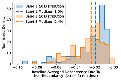
Figure 12: Following H22a, we show here our estimate for signal loss due to non-redundancy while forming and averaging cross-baseline power spectra within redundant baseline groups. Our metric $\Delta\kappa$, defined in Equation 10, looks at the difference between the power in an incoherent average and a coherent average over baselines. We compute those powers at $\tau=0$, the delay of sources at zenith, as a proxy for cosmological signal loss in the main beam. As in H22a, that difference is normalized by the incoherently-averaged power smoothed on 1 hour timescales to minimize the effect of nulls. This quantity is then weighted by the inverse noise variance, and we show here the histogram over unique baselines and over our five fields. Taking the median of this histogram, we estimate a 1.9% correction for Band 1 and a 2.4% correction for Band 2, as we discuss in Section 3.3.6.

H22a performed this analysis over a short range of LSTs around the galactic plane crossing (7.2–8.3 hours) and found a $\sim$1% signal loss due to decoherence. We measure $\Delta\kappa$ by taking a median over a wider range of LSTs—all five fields—in part to account for LST- or JD-dependent gain errors and the possibility that the array became more or less redundant over the season. Assuming that the signal loss due to non-redundancy should relatively be stable in LST, and with the knowledge that nulls in power on certain baselines can create spurious temporal outliers in $\Delta\kappa$ that always create extra apparent decoherence, even with the 1-hour smoothing, we take the median of this histogram as our signal loss estimate. This yields a slightly larger estimate of the loss: 1.9% for Band 1 and 2.4% for Band 2. This will be accounted for in our final power spectrum upper limits, as we will discuss presently.

3.3.6 Correcting for Potential Biases and Signal Loss

H22a performed a careful accounting for four potential sources of bias in the final power spectrum. Three of these are forms of signal loss—ways in which true sky power from the 21 cm signal can be removed due to the analysis choices we made. The fourth, due to absolute calibration, produced an overall bias in H22a that affected both our measured power spectrum and also our noise and error estimates, which are ultimately derived from autocorrelations which were also biased (Aguirre et al. 2022). Each of these corrections was applied separately per band.

In Table 2, we report all of the per-band bias corrections used in this work.

Table 2: Summary of fractional signal power lost over the course of the analysis. The effect of non-redundancy is estimated from the data directly (Section 3.3.5); the rest are derived from simulations of sky signal, noise, and instrumental systematics (Section 4).

Potentially Lossy or Biased Analysis Step	Band 1 ($z=10.4$)	Band 2 ($z=7.9$)
Absolute calibration	$\lesssim 0$%	$\lesssim 0$%
Crosstalk subtraction	2.4%	3.3%
Coherent time-averaging in LST	1.2%	1.5%
Redundant-baseline averaging	1.9%	2.4%
Total signal loss correction	5.5%	7.2%

The corrections for crosstalk subtraction, coherent time averaging, and redundant-baseline averaging are all forms of signal loss that do not affect our autocorrelations and thus our estimate of the thermal noise $P_{N}$ (though they can have a small effect on $\hat{P}_{SN}$). All these effects are taken into account when reporting power spectra, errors, and upper limits in Section 5.

We discussed our evaluation of the signal loss due to non-redundancy in Section 3.3.5. The other three sources of bias are quantified using the realistic sky and instrument simulations we use to validate our analysis pipeline, as we discuss in Section 4. The first two, signal loss due to coherent time averaging and signal loss due to crosstalk subtraction, are evaluated in simulations performed without noise in order to precisely measure the effect on a known EoR-like signal in Section 4.3. As discussed in Section 3.2.2, the absolute calibration bias that was due to the effect of low-SNR visibilities should have been eliminated in this work. Indeed, we will show in Section 4.2 that the effect has been reduced in magnitude to less than 1% in the gains, and has reversed sign—our gains now appear to be biased very slightly low. If this is correct, then that would lead to an overestimate of our power spectra, error bars, and upper limits. Since we are far more concerned with the possibility of signal loss leading us to report an upper limit lower than the data justify, we choose conservatively not to adjust for this effect in the limits we report in Section 5.

4 Analysis Pipeline Validation with Simulations

Before we present our final upper limits in Section 5, we first report the results of our extensive simulation-based validation of the analysis pipeline. The techniques used for simulating our instrument and the analyses performed on the output of those simulations are very similar to those in Aguirre et al. (2022), which was written to support H22a. We present here a brief summary of how we applied those techniques to this work, highlighting the relevant updates, and then show some key results that both validate the overall pipeline and help us to quantify specific signal loss biases that we correct for (see Section 3.3.6).

4.1 Visibility and Systematics Simulations

Our primary method for validating the analysis pipeline presented in Section 3 is via an end-to-end simulation, wherein we generate realistic visibility simulations of foregrounds, noise, and a boosted EoR-like signal that should be easily detectable given our sensitivity. This allows us to holistically evaluate the performance of the analysis and identify any unknown sources of bias. One could also approach the same problem by injecting a signal of known amplitude (larger than the real EoR) into the visibilities and analyzing that data in the same way. However, this technique requires high confidence in one’s calibration solutions (injected visibilities must be “uncalibrated” before injection) and it is difficult to disentangle residual systematics form power spectrum biases.

Our sky simulations consist of three unpolarized components: diffuse Galactic emission, a point source catalog, and an EoR analogue created as a Gaussian random field drawn from a known power spectrum. We present each of these here and discuss how they differ from the corresponding components in Aguirre et al. (2022). For the diffuse Galactic emission, we use the Global Sky Model (GSM; de Oliveira-Costa et al. 2008), computed at every frequency we measure using pygdsm. The result is a HEALPix map (Górski et al. 2005) with resolution $N_{\text{side}}=512$. We smooth the map with a $1^{\circ}$ Gaussian kernel and degrade it to $N_{\text{side}}=128$ to speed up our simulations, since that provides sufficient resolution to cover the angular scales HERA is sensitive to. Each HEALPix pixel is treated as a single point source at its center using the pixel area for normalization.

Our model of point source emission differs significantly from Aguirre et al. (2022) in our handling of spatial gaps in the MWA GLEAM catalog (Hurley-Walker et al. 2017) due to the Galactic plane. Since H22a used observations spanning a much smaller range of LSTs than those used in this work, it was decided to slightly further restrict the range of LSTs simulated to 1.5–7 hours in order to avoid those gaps. In this work, we wanted to be able to simulate the full 24 hours of LST, so we developed a GLEAM-analogue with simulated point sources. We created 14,073,688 random synthetic sources with uniformly random positions across the sky. Their fluxes were drawn to match the GLEAM source count distribution in Franzen et al. (2019) from 0.001–87 Jy. Their spectral indices were drawn from a Gaussian distribution with mean $-0.79$ and standard deviation 0.05, again following Franzen et al. (2019) (see also, e.g., Offringa et al. 2016; Carroll et al. 2016). The 200,000 brightest sources were simulated at their random positions, the remainder (those below 0.1975 Jy) were treated as confusion noise. For the sake of computational expediency, these were added to the GSM at the nearest HEALPix grid point. Above 87 Jy, we added a several real sources in their true positions. This includes GLEAM J215706-694117, GLEAM J043704+294009, GLEAM J122906+020251, GLEAM J172031-005845, and the “A-Team” sources reported in Table 2 of Hurley-Walker et al. (2017). We also include Fornax A, which we model as a single 750 Jy source with a spectral index of $-0.825$ at a right ascension of 3${}^{\text{h}}$22${}^{\text{m}}$42${}^{\text{s}}$ and a declination of $-37^{\circ}$12${}^{\prime}2^{\prime\prime}$ (McKinley et al. 2015).

Finally, our boosted EoR analogue is created with the same simulator used in Aguirre et al. (2022). We used a higher amplitude mock EoR and a slightly different power spectrum slope: $P(k)\propto k^{-2.7}$. That EoR simulation was binned to the same HEALPix grid as the diffuse foregrounds, where again each pixel center is treated as a point source.

To actually simulate visibilities, we use vis_cpu (Bull 2021), a fast visibility simulator validated against pyuvsim (Lanman et al. 2019), a reference simulator designed for accuracy (Pascua et al. in prep.). The simulator used in Aguirre et al. (2022), RIMEz, calculates visibilities in spherical harmonic space. vis_cpu takes a much simpler approach. It calculates a per-antenna visibility factor for each point-like sky component—essentially the square root of the source flux with a phase factor that depends on frequency and antenna position—and multiplies them by a Jones matrix. These are then cross-multiplied to form visibilities and summed over sources. We use the primary beam calculated in Fagnoni et al. (2021) and interpolated in azimuth and zenith angle. We simulate the full 24 hours of LST at a five second cadence for each unique baseline and frequency observed by HERA.

Our end-to-end validation began with producing two sets of 94 nights of simulated data, one with the mock boosted EoR and one without. Both included foregrounds, noise, and systematics. For each night, we interpolated the original set of simulated visibilities using a cubic spline onto each night’s 10.7 second cadence, since the LST grid of the data varied from night to night. Unlike in Aguirre et al. (2022), where we used only a subset of the antennas, in this work we inflated the redundant baselines to produce data files with all baselines not flagged in the real data. The final simulated data set completely matched the real data in terms of baselines, times, and frequencies. No non-redundancy due to antenna-to-antenna variation of beams or positions offsets (Orosz et al. 2019; Dillon et al. 2020; Choudhuri et al. 2021) was simulated.

We then “uncalibrate” the data by applying per-antenna complex bandpasses and cable reflection terms and then add noise to the visibilities, both steps performed exactly the same way as in Aguirre et al. (2022). Finally, our simulations have per-baseline crosstalk added to them. Again, this is done with nearly the same procedure as in the prior validation work. For each baseline, we model the crosstalk as a series of copies of the autocorrelation of each antenna in the baseline, each multiplied by a complex delay term and an amplitude that decreases exponentially with delay by a factor of 100 from the peak delay out to 2000 ns. In this work, the amplitudes and delays of the crosstalk peak, and how they depend on position in the array, are motivated by the new physical model of the crosstalk (see Appendix A) in which we attribute crosstalk to an emitter on the west side of the array. (In our model we use $\alpha=-2.29$ and $\tau_{\rm offset}=0$ ns; see Equation A4 for definitions.) The crosstalk structure is allowed to change per epoch, but not per night. The amplitudes are on the low end of what is observed in real data in order to avoid cross-talk effects on certain baselines becoming crosstalk-dominated, since the visibility simulation itself is also somewhat underpowered on long baselines relative to the real sky. We do not explicitly model any of the multipath effects hypothesized to be responsible for the breadth of the crosstalk spectrum, relying instead on that series of peaks as in Aguirre et al. (2022). All of the techniques for visibility corruption, along with an interface to vis_cpu, are packaged into hera_sim.

4.2 Validation Results from End-to-End Simulations

With our procedure for turning visibility simulations into full nights of “uncalibrated,” systematics-corrupted data matching the real data, we then apply our analysis pipeline almost exactly as described in Section 3. We perform redundant-baseline calibration and absolute calibration, then flag, then smooth our gain solutions. We next bin together individual epochs and perform inpainting, cable reflection calibration, and crosstalk subtraction. After binning together the four epochs, we form pseudo-Stokes visibilities, time-average, and estimate power spectra. We run the entire end-to-end pipeline twice—once without the mock EoR and once with it—including the various power spectrum cuts described in Section 3.3. In order to faithfully validate the analysis pipeline, the same software packages—pyuvdata (Hazelton et al. 2017), hera_cal, hera_qm, and hera_pspec—with the same git hashes that were used to run the end-to-end validation.

The one major step that was performed differently was RFI flagging. Following Aguirre et al. (2022), we do not inject RFI and then attempt to detect it. Rather, we simply cross-apply the real data’s flags to the simulated data at the same step in the pipeline. Since the times, frequencies, and baselines match perfectly, this step is very straightforward. Likewise, we take the final flagging mask generated from a manual inspection of the data (see Section 3.2.3) and apply it to each epoch of simulated data at precisely the same point in the real pipeline that those flags are applied to real data.

Before we discuss the final power spectra, we can now evaluate whether the fix offered in Section 3.2.2 eliminates the bias in absolute calibration discovered in Aguirre et al. (2022) and corrected for in H22a. In Figure 13, we compare the calibration solutions produced by the pipeline for Epoch 1 (the longest epoch) with the known simulated gains, averaging over antennas, times, and nights.

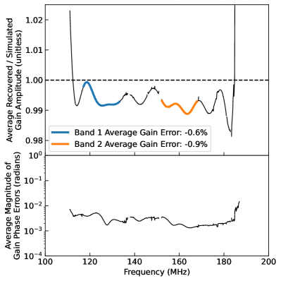
Figure 13: In our end-to-end tests with simulated data, we can compare the known input gains to the derived gains after redundant-baseline calibration, absolute calibration, and calibration smoothing. Here we show the average gain errors after averaging over antennas, times, and nights for Epoch 1, the longest epoch. In the bottom panel, we show the error in our gain phases; these are comparable to those found in the validation of our H22a limits in Aguirre et al. (2022). In the top panel we show our gain amplitude errors. These are substantially smaller than those found in Aguirre et al. (2022) due to our new algorithm for absolute amplitude calibration which is not biased when visibility SNR is low (see Section 3.2.2 for details). In the bands of interest, our gains are correct to within 1%. While we do have some evidence that they are biased slightly low, which would lead to a power spectrum that is slightly too high, we choose conservatively to not to adjust the power spectrum to compensate (see Section 3.3.6).

By comparison to Figure 11 of Aguirre et al. (2022), we can see that the absolute calibration bias is largely eliminated and that the phases are still well-recovered across the band. The gain errors are largest at the band edges, due to edge effects of the low-pass filter used in gain smoothing.

Interestingly, we actually now see a slight negative bias for most frequencies (0.6% for Band 1, 0.9% for Band 2), which could lead to overestimating power spectra and error bars by a few percent, since gain errors impact power spectra quartically. One possible origin of the effect is a rare failure mode of the absolute calibration bias fix described in Section 3.2.2. When fitting for a single overall amplitude, solutions are biased but quite stable in time. When fitting for a complex number and then taking the absolute value of that, we have seen rare instances where the data and reference visibilities are so far apart that the gains are driven to 0 in order to minimize $\chi^{2}$. In real data, these sorts of collapses are easily identified as discontinuities and flagged as RFI. This justifies our conservative choice in Section 3.3.6 to not correct for any remaining absolute calibration bias since we do not expect this effect to be as large on our final upper limits. However, in our end-to-end pipeline validation, we flag precisely where we did in the real data, ignoring any potential new discontinuities. These artificially low gains can thus be the consequence of a rare calibration failure getting spread out and diluted by gain smoothing.

We turn now to the final result of our end-to-end test: spherically-averaged power spectra for both bands and all five fields, with and without our mock boosted EoR. In Figure 14, we show one field for each band (corresponding to our lowest limits, see Section 5).

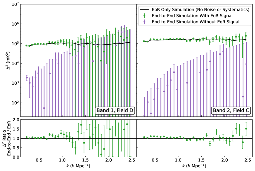
Figure 14: Here we show the final result of our end-to-end test of our data reduction pipeline on simulated data. We simulated visibilities both with (green) and without (purple) a boosted EoR analogue Gaussian random field, along with foregrounds, noise, and instrumental systematics, for all 94 nights. (For visual clarity, the points along the $k$ axis were slightly off set between green and purple.) This was then processed with almost all the same code as was used to process the real data in order to thoroughly test our analysis chain. As the bottom panels showing the ratio of our end-to-end-test (the green points) to the particular boosted mock EoR realization (black solid line), our results match the EoR realization quite well. There is no evidence for additional signal loss not accounted for in Section 3.3.6. While this calculation was performed for all bands and fields, we show here just the two fields where our lowest limits are derived at each band (see Section 5).

The power spectra include signal loss corrections for crosstalk subtraction and coherent time averaging, as described in Section 3.3.6, but no correction for non-redundancy as none is included in the simulation. For comparison, we also show the results of a simulation run with only the mock EoR with no foregrounds, noise, systematics, or flags (black line). It is interpolated directly onto the grid of the final LST-binned data set, time-averaged, converted to pseudo-Stokes I, and formed into power spectra.

In general, we find the results of our end-to-end test in good agreement with the mock EoR-only power spectrum, as the bottom panels of Figure 14 show. Though the error bars on the power spectrum with EoR signal may be underestimates (since sample variance is not accounted for in our real pipeline), there is no evidence for an additional, unaccounted-for contribution to signal loss that might lead us to report artificially low upper limits. If anything, we see some evidence that our results are biased slightly high. This is likely due to a number of factors; the bias high due to rare absolute calibration failures, a possible overestimation of the impact of signal loss, and the effect of flagging and inpainting. When the same pipeline is run without the EoR, the results are consistent with noise at almost all $k$—a result of the somewhat aggressive cuts we discuss in Section 3.2.4 and Section 3.3.3—though we unsurprisingly do see some residual foregrounds at very low $k$, especially in Band 1. This is consistent with what we see in the real data in most fields (see Section 5.2).

4.3 Noise-Free Tests for Quantifying Potential Signal Loss

Separately from our end-to-end simulations, we also repeat two tests of signal loss performed in Aguirre et al. (2022) that were used in H22a to correct the final power spectrum measurements (see Section 3.3.6). The first is the effect of coherently time-averaging LST-binned visibilities from 21.4 s to 214 s before cross-multiplying interleaved visibilities to form power spectra. This is done by interpolating mock EoR-only visibilities onto the 21.4 s grid of the final LST-binned data set, forming pseudo-Stokes I, and then either forming power spectra directly or forming power spectra after coherently averaging to a 214 s cadence with rephasing as described in Section 3.1. If we take the result with 21.4 s integrations to be loss-free, which it should be to a good approximation, then we find a 1.2% signal loss for Band 1 and a 1.5% signal loss for Band 2 (see Figure 15).

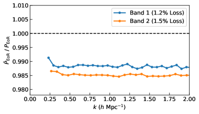
Figure 15: Here we repeat the test of decoherence from time-averaging shown Figure 17 of Aguirre et al. (2022). We compare power spectra computed from EoR-only visibility simulations at a 21.4 s cadence—which is what we obtain after LST-binning—to the same data averaged to a 214 s cadence before forming power spectra. After averaging over all fields and baselines, we find a result in agreement with Aguirre et al. (2022). In H22a, the two bands are averaged together and the effect is taken to be a 1% correction; here we keep the two bands separate to arrive at our signal loss correction factors (see Section 3.3.6 and Table 2).

It is not surprising that the signal loss should be slightly higher for Band 2, since the primary beam is smaller at higher frequencies and the rephasing of visibilities before averaging cannot account for the changing beam-weighted sky. Likewise, if we were to open up additional degrees of freedom in our signal loss correction, we would likely find that this decoherence depends on baseline length and orientation—baselines that fringe more quickly should see more loss here. Since we are using the same weighting of baselines here as in analysis of the real data, the overall loss estimate should be correct to first order. Therefore, because the overall signal loss is quite small, it is not necessary to further complicated the signal loss correction by making it baseline dependent. Regardless, these values are consistent with the 1% loss figure used in H22a and calculated in Aguirre et al. (2022), which did not separate out the two bands.

The second specialized test is to examine the impact of crosstalk subtraction (described above in Section 3.1 and Section 3.2.4). The crosstalk subtraction algorithm devised in Kern et al. (2019), demonstrated in Kern et al. (2020b), and employed for H22a removes power near fringe-rate zero. The maximum extent of this removal in fringe-rate space (Equation 3) is designed to keep signal loss at the $\sim$1% level. To measure this effect, we interpolate to get one data set per epoch with foregrounds, mock EoR, and crosstalk injected, but no noise or calibration errors. To this data set we apply our final flagging mask, inpaint, subtract cross-talk, LST-bin the four epochs together, form pseudo-Stokes visibilities, coherently time-average, and then form power spectra. We spherically average those power spectra over baselines using the same noise-based weights as were applied to the data. In Figure 16, we compare those per-time-step power spectra to mock EoR-only power spectra with the same averaging performed. We take a median over delay up to 4000 ns, the highest delay in the crosstalk subtraction SVD, to produce a single bias estimate per LST and per band. As H22a argues, we expect the crosstalk subtraction bias to scale-independent.

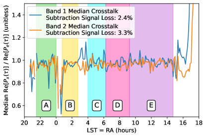
Figure 16: Our final test of potentially biasing signal loss examines the effect of our crosstalk subtraction algorithm on the EoR signal. Here we compare simulations with just our boosted EoR model—the numerator in Figure 15—to noise-free, per-epoch simulations with EoR, foregrounds, and crosstalk systematics. Crosstalk subtraction is performed on a per-epoch basis, after which epochs are combined, formed into power spectra, and then averaged as usual to get spherical power spectra as a function of time. Taking the median over delays less than 4000 ns and LSTs in our five fields, we estimate 2.4% loss in Band 1 and 3.3% loss in Band 2, which we report in Table 2.

The final result is a bit difficult to interpret. Clearly the result is LST-dependent; just as in Aguirre et al. (2022), we see higher levels of signal loss near gaps in the data—this was one of the reasons we avoided the range from 0–0.75 hours of LST. We also see some evidence under-subtraction around Fornax A (in Band 1) and the Galactic center, though the latter is expected due the weighting in the SVD. To avoid the effect of outliers in both directions, we estimate our per-band signal loss by taking the median over LSTs in the five fields. This yields 2.4% signal loss in Band 1 and 3.3% loss in Band 2, which is basically consistent with the 1% and 3% used in H22a.

5 Upper Limits on the 21 cm Power Spectrum

Having surveyed our technique for reducing 94 nights of visibilities to our final power spectra, and having validated that technique and quantified the signal loss biases we must correct for, we are finally in a position to present our upper limits on the 21 cm EoR power spectrum.

5.1 Cylindrically-Averaged Power Spectra

We begin with cylindrically-averaged power spectra. These are first averaged over all cross-baseline pairs within each redundant baseline group (excluding those with high residual crosstalk, see Section 3.2.4). Next they are averaged incoherently in time over each field. Finally, they are incoherently averaged in $|\mathbf{u}|$, combining together baselines with the same length. All averages use $P_{N}$ (Equation 6) to perform inverse variance weighting; $P_{N}$ and $\hat{P}_{SN}$ (Equation 7) errors are propagated during each step. This produces power spectra in $\tau$ and $u$, which is equivalent in the delay approximation to $k_{\|}$ and $k_{\perp}$ (Parsons et al. 2012a). These cylindrical power spectra are the most sensitive data products that still keep $k_{\|}$ and $k_{\perp}$ separate, which is useful because different scales along those two axes are measured in a fundamentally different way instrumentally and correspond to different ways of measuring distance cosmologically. While we are not yet sensitive enough to constrain the cosmological signal’s dependence on line-of-sight velocity effects, cylindrical power spectra are still useful for evaluating how foregrounds and other systematics appear upon deep integration.

We show our cylindrically-averaged power spectra for each of the five fields in Figure 17 for Band 1 and Figure 18 for Band 2.

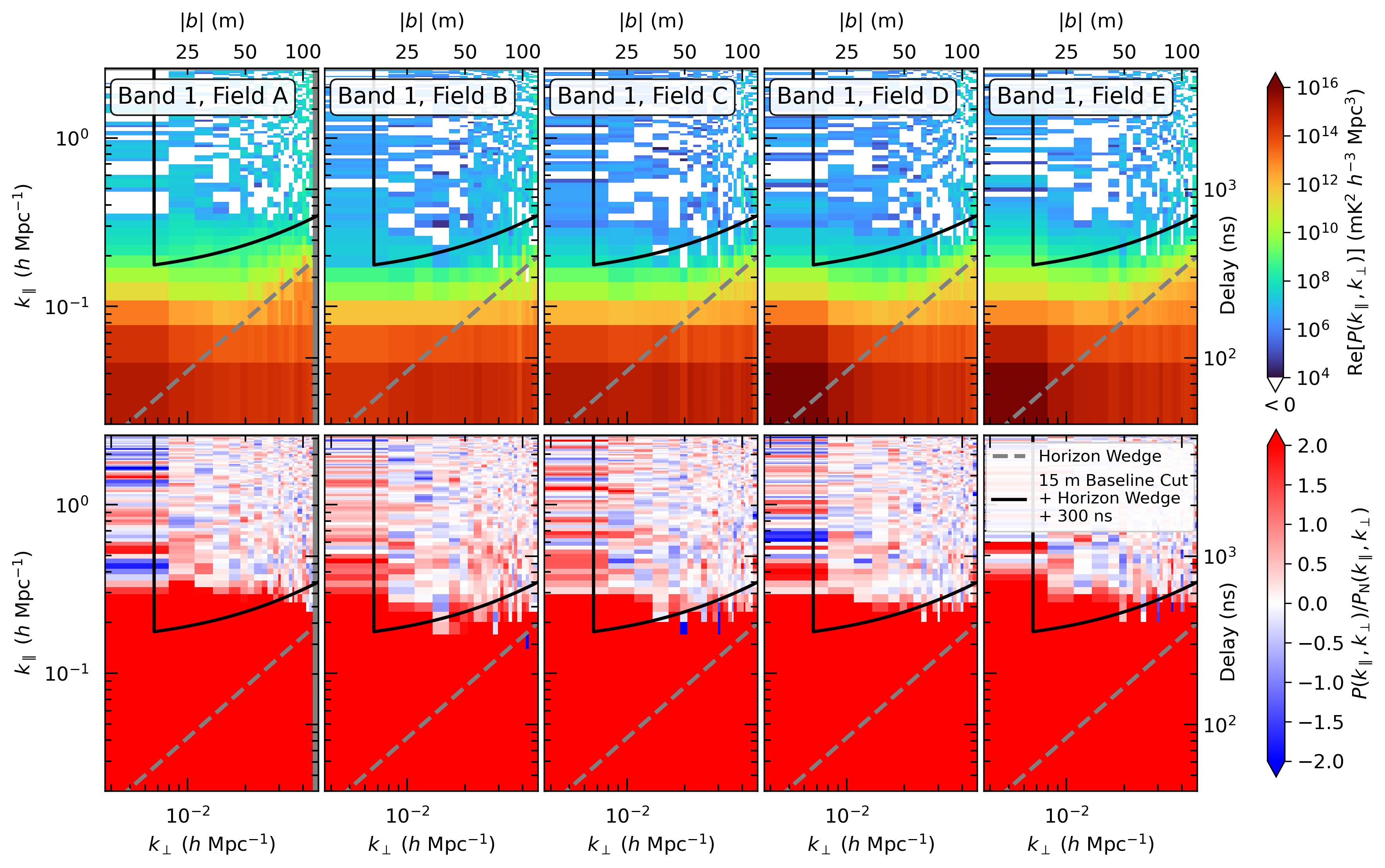
Figure 17: Here we show our cylindrically-binned power spectra for all five fields for Band 1 ($z=10.4$). In the top row, we show the real part of $P(k)$; in the bottom row, we show the same power spectra normalized by the power spectrum of expected noise. Since noise-dominated regions of this space are equally likely to be positive or negative, we can see that most of the EoR window is noise-dominated. These power spectra are formed by averaging together all cross-baseline pairs within a redundant baseline group and then by incoherently averaging in time in each field. Both averages are performed with inverse noise variance weighting. We convert from baseline and delay to $k_{\perp}$ and $k_{\|}$ respectively using the delay spectrum approximation (Parsons et al. 2012a). Note that bins that fall below the horizon wedge (Equation 8) plus a 300 ns buffer, along with baselines with projected east-west distances less than 15 m, are included here to help illustrate systematics but are excluded from all spherically binned power spectra.

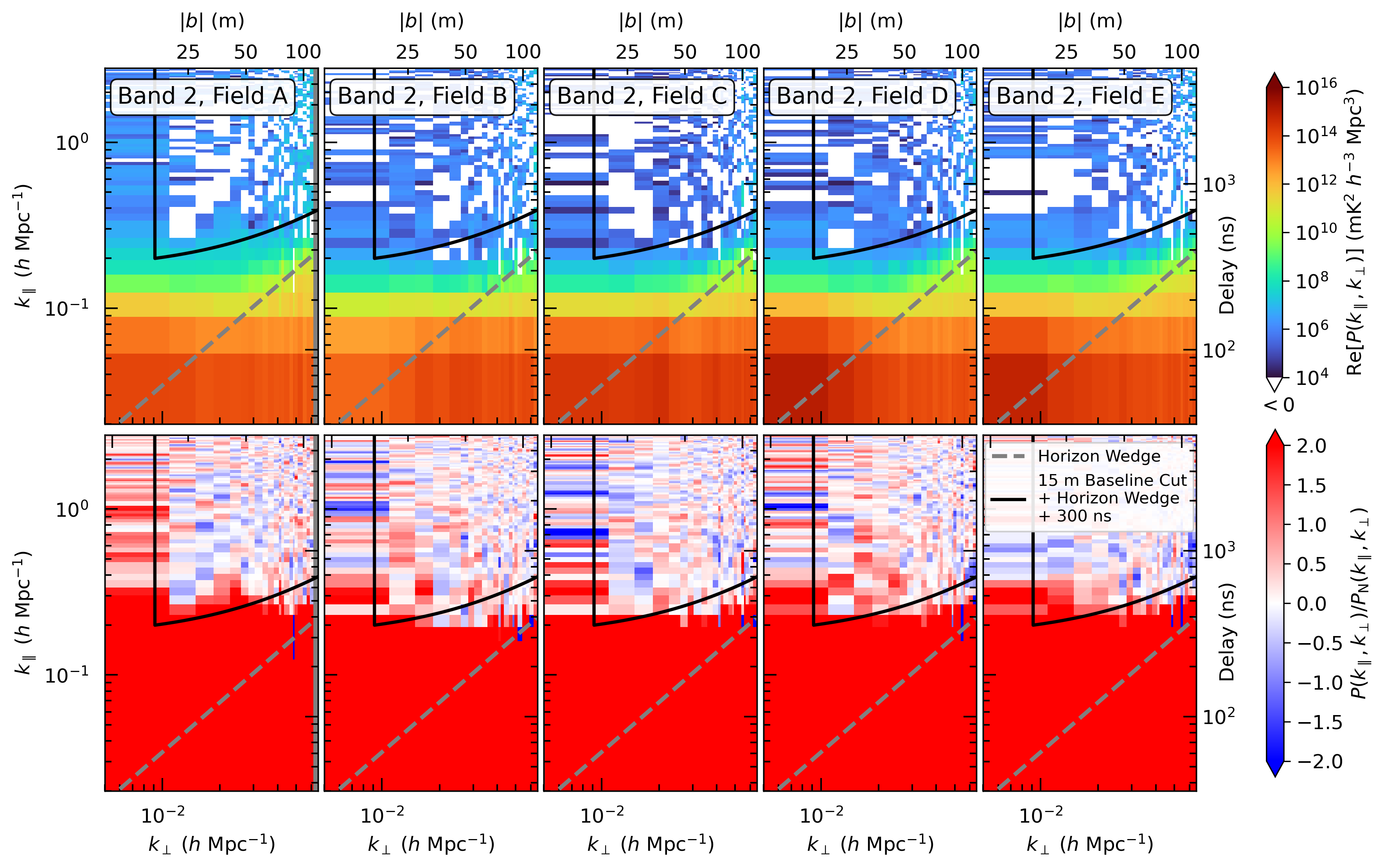
Figure 18: The same plot of cylindrically-binned $P(k)$ and SNRs as in Figure 17, but for Band 2 ($z=7.9$).

In the top row of each figure, we show the real part of the power spectrum. We also show the power spectrum SNR, $P/P_{N}$ in the bottom row. In regions that are noise-dominated, we expect roughly half of the power spectrum bins to be negative (white) and we expect the SNR to have mean 0 and standard deviation 1.

What we see is fairly consistent with that expectation across most of the EoR window. However, the foreground-dominated region clearly extends well beyond the horizon wedge (gray dashed line). This justifies the need for a buffer beyond the horizon wedge and our choice specifically to expand it from 200 ns as in H22a to 300 ns (black solid line). As we discussed in Section 3.3.3, our choice of the buffer was set by examining these SNR plots and trying to balance the amount of foreground leakage into the window at low $k_{\perp}$ with the amount of noise-dominated modes excised at high $k_{\perp}$.

Note that a number of data points that we excise from our spherically-averaged power spectra are still shown in Figure 17 and Figure 18. We have not yet removed the modes under the horizon wedge and buffer, nor have we removed baselines with projected east-west distance less than 15 m (though baselines with a projected east-west distance less than 14 m have already been removed because crosstalk subtraction could not be performed on them without substantial signal loss, see Section 3.1).

5.2 Spherically-Averaged Power Spectra and the Deepest Upper Limits

We now turn to our spherically-averaged power spectrum measurements and upper limits. These are produced from averaging together all baselines incoherently after excising modes below the horizon wedge (Equation 8) plus a 300 ns buffer and all baselines with a projected east-west length less than 15 m (which includes the single-unit east-west spacing; see Figure 4). The result, for all bands and fields, is shown as a “dimensionless” power spectrum (Equation 5) in Figure 19.

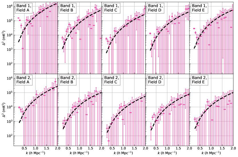
Figure 19: Our final limits on the 21 cm brightness temperature power spectra $\Delta^{2}(k)$, for all five fields and both Band 1 ($z=10.4$) and Band 2 ($z=7.9$). The points are the real parts of the bandpowers. The vertical error bars are 2$\sigma$ and the black dashed lines denote 1$\sigma$ errors. The horizontal error bars denote the range from the 16th to the 84th percentile of the window functions. Upper limits derived from negative measurements are conservatively set at $2\sigma$; all other limits are set at $\Delta^{2}(k)+2\sigma$. Any points whose error bars pass through the y-axis are consistent with noise at 2$\sigma$. Our lowest 2$\sigma$ upper limits are 3,496 mK² at 0.36 $h$Mpc^-1 in Band 1, Field D and 457 mK² at 0.34 $h$Mpc^-1 in Band 2, Field C. The precise values of the power spectrum, error bars, and upper limits at low $k$ are reproduced in Table 3 and Table 4. Following H22a, we leave the incoherent averaging of different fields together for future work.

We estimate vertical errors by propagating $\hat{P}_{SN}(k)$ (Equation 7) and show the measurements $\pm 2\sigma$ after converting to $\Delta^{2}$ using Equation 5. When measurements are negative, we adopt the strong prior that the true power spectrum must be zero or positive and plot upper limits at precisely $2\sigma$. The $1\sigma$ error level derived from $\hat{P}_{SN}(k)$ is shown as a black dashed line. Our absolute lowest $2\sigma$ upper limits on the power spectrum are $\Delta^{2}(k=\text{0.36\,$h$Mpc${}^{-1}${}})\leq\text{3,496\,mK${}^{2}${}}$ at $z=10.4$ (Band 1, Field D) and $\Delta^{2}(k=\text{0.34\,$h$Mpc${}^{-1}${}})\leq\text{457\,mK${}^{2}${}}$ at $z=7.9$ (Band 2, Field C). These limits are 2.6 and 2.1 times deeper, respectively, than those presented in H22a. We report the measured power spectra, $1\sigma$ error bars, and and $2\sigma$ upper limits results at most values of $k$—including low $k$, which is where most of our astrophysical constraining power comes from—in Table 3 for Band 1 and Table 4 for Band 2.

Table 3: Band 1 ($z=10.4$) power spectra, errors, and upper limits from Figure 19. The upper limit is taken to be $2\sigma$ above the power spectrum measurement or above 0, whichever is greater. The lowest upper limit is in bold.

	$k$	$\Delta^{2}$	$1\sigma$	$\Delta^{2}_{\rm UL}$	$k$	$\Delta^{2}$	$1\sigma$	$\Delta^{2}_{\rm UL}$	$k$	$\Delta^{2}$	$1\sigma$	$\Delta^{2}_{\rm UL}$
	$(h\ {\rm Mpc}^{-1})$	$({\rm mK})^{2}$	$({\rm mK})^{2}$	$({\rm mK})^{2}$	$(h\ {\rm Mpc}^{-1})$	$({\rm mK})^{2}$	$({\rm mK})^{2}$	$({\rm mK})^{2}$	$(h\ {\rm Mpc}^{-1})$	$({\rm mK})^{2}$	$({\rm mK})^{2}$	$({\rm mK})^{2}$
Field A	0.23	153,691	2,933	159,556	0.73	-32,771	58,377	116,753	1.22	588,465	274,340	1,137,146
	0.29	107,667	4,271	116,208	0.79	61,900	74,547	210,994	1.28	406,694	318,088	1,042,869
	0.36	45,688	7,105	59,898	0.85	43,307	93,159	229,625	1.35	669,812	366,722	1,403,255
	0.42	1,182	11,336	23,854	0.91	158,855	115,453	389,760	1.41	-22,002	418,809	837,617
	0.48	-6,756	17,231	34,462	0.97	-2,569	140,221	280,442	1.47	721,387	476,106	1,673,599
	0.54	28,245	24,666	77,577	1.04	-25,200	167,921	335,842	1.53	190,383	537,247	1,264,877
	0.60	115,543	33,997	183,537	1.10	-206,058	199,136	398,273	1.59	-63,312	604,314	1,208,628
	0.66	101,535	45,017	191,569	1.16	412,511	235,335	883,180	1.65	440,694	676,991	1,794,676
Field B	0.23	6,414	878	8,169	0.73	-16,887	19,741	39,482	1.22	-3,270	90,946	181,893
	0.29	3,352	1,343	6,038	0.79	38,162	25,246	88,654	1.28	-23,054	105,349	210,698
	0.36	4,815	2,346	9,506	0.85	14,007	31,608	77,223	1.35	208,370	121,329	451,027
	0.42	18,593	3,852	26,297	0.91	103,161	38,899	180,959	1.41	312,314	138,131	588,576
	0.48	26,651	5,896	38,443	0.97	117,071	46,962	210,995	1.47	52,833	157,295	367,424
	0.54	54,508	8,475	71,457	1.04	5,188	55,544	116,277	1.53	28,767	178,728	386,224
	0.60	30,557	11,578	53,714	1.10	-21,580	66,145	132,291	1.59	202,144	200,619	603,381
	0.66	6,089	15,308	36,705	1.16	-38,769	77,809	155,618	1.65	46,875	225,195	497,265
Field C	0.23	5,565	472	6,509	0.73	-5,911	10,003	20,006	1.22	101,849	46,514	194,876
	0.29	3,763	687	5,137	0.79	-1,040	12,731	25,461	1.28	-42,117	53,624	107,247
	0.36	1,525	1,185	3,895	0.85	-555	15,963	31,926	1.35	109,485	62,018	233,520
	0.42	6,806	1,993	10,793	0.91	-35,281	19,656	39,312	1.41	-59,321	70,760	141,521
	0.48	-6,007	3,067	6,134	0.97	-51,204	23,825	47,651	1.47	-42,848	80,462	160,924
	0.54	-7,550	4,320	8,641	1.04	-27,920	28,398	56,795	1.53	148,253	90,978	330,208
	0.60	19,718	5,898	31,514	1.10	43,689	33,761	111,212	1.59	227,669	102,654	432,978
	0.66	18,353	7,755	33,864	1.16	43,764	39,661	123,085	1.65	130,546	114,700	359,945
Field D	0.23	13,006	677	14,360	0.73	-11,090	14,727	29,454	1.22	197,836	68,914	335,664
	0.29	2,325	1,011	4,347	0.79	-5,471	18,791	37,582	1.28	-45,122	79,627	159,254
	0.36	-207	1,748	3,496	0.85	-29,815	23,439	46,878	1.35	62,242	91,821	245,885
	0.42	6,866	2,888	12,643	0.91	-21,743	29,005	58,010	1.41	-95,510	105,107	210,215
	0.48	-1,255	4,423	8,846	0.97	26,219	35,219	96,657	1.47	158,372	119,620	397,612
	0.54	25,094	6,301	37,696	1.04	18,461	42,035	102,530	1.53	69,220	134,761	338,742
	0.60	17,496	8,595	34,687	1.10	112,195	50,065	212,326	1.59	-3,969	151,666	303,332
	0.66	14,751	11,370	37,490	1.16	-46,370	58,914	117,827	1.65	-256,395	169,976	339,953
Field E	0.23	28,531	957	30,444	0.73	-29,956	20,066	40,133	1.22	-4,695	94,165	188,330
	0.29	14,846	1,394	17,634	0.79	27,200	25,575	78,350	1.28	70,547	109,087	288,722
	0.36	6,793	2,382	11,557	0.85	45,734	32,039	109,812	1.35	32,410	125,598	283,606
	0.42	2,510	3,946	10,401	0.91	2,109	39,559	81,228	1.41	220,926	143,720	508,367
	0.48	-2,082	6,016	12,031	0.97	48,558	48,118	144,795	1.47	129,091	163,068	455,227
	0.54	8,265	8,530	25,324	1.04	-99,003	57,725	115,450	1.53	370,465	185,109	740,683
	0.60	-21,997	11,634	23,267	1.10	-58,513	68,608	137,217	1.59	153,201	207,953	569,107
	0.66	14,858	15,432	45,722	1.16	-78,339	80,512	161,025	1.65	175,314	232,387	640,089

Table 4: Band 2 ($z=7.9$) power spectra, errors, and upper limits from Figure 19. The upper limit is taken to be $2\sigma$ above the power spectrum measurement or above 0, whichever is greater. The lowest upper limit is in bold.

	$k$	$\Delta^{2}$	$1\sigma$	$\Delta^{2}_{\rm UL}$	$k$	$\Delta^{2}$	$1\sigma$	$\Delta^{2}_{\rm UL}$	$k$	$\Delta^{2}$	$1\sigma$	$\Delta^{2}_{\rm UL}$
	$(h\ {\rm Mpc}^{-1})$	$({\rm mK})^{2}$	$({\rm mK})^{2}$	$({\rm mK})^{2}$	$(h\ {\rm Mpc}^{-1})$	$({\rm mK})^{2}$	$({\rm mK})^{2}$	$({\rm mK})^{2}$	$(h\ {\rm Mpc}^{-1})$	$({\rm mK})^{2}$	$({\rm mK})^{2}$	$({\rm mK})^{2}$
Field A	0.27	9,331	649	10,628	0.83	-14,403	14,954	29,908	1.40	63,705	68,760	201,225
	0.34	6,479	1,027	8,532	0.90	12,644	18,997	50,637	1.47	104,906	79,266	263,438
	0.41	4,731	1,774	8,279	0.97	-7,283	23,849	47,699	1.54	-115,042	91,161	182,322
	0.48	-2,629	2,857	5,713	1.05	76,346	29,519	135,384	1.61	-93,039	104,349	208,699
	0.55	1,803	4,376	10,556	1.12	-4,423	35,449	70,899	1.68	-80,538	118,562	237,124
	0.62	-12,812	6,296	12,592	1.19	-95,045	41,893	83,785	1.75	227,088	134,070	495,227
	0.69	-2,143	8,621	17,243	1.26	-19,638	49,987	99,974	1.83	157,690	151,649	460,988
	0.76	-4,635	11,486	22,973	1.33	-44,250	58,807	117,614	1.90	576,790	169,926	916,643
Field B	0.27	747	229	1,204	0.83	10,939	5,601	22,140	1.40	61,788	25,729	113,245
	0.34	1,149	377	1,902	0.90	4,164	7,130	18,424	1.47	48,349	29,834	108,017
	0.41	-770	657	1,314	0.97	24,889	8,943	42,774	1.54	23,599	34,335	92,268
	0.48	1,254	1,080	3,415	1.05	10,417	11,027	32,470	1.61	15,477	39,195	93,868
	0.55	-1,770	1,655	3,310	1.12	-33,006	13,209	26,418	1.68	52,495	44,690	141,876
	0.62	1,916	2,369	6,654	1.19	-11,140	15,659	31,319	1.75	125,943	50,570	227,083
	0.69	9,099	3,231	15,562	1.26	33,775	18,651	71,077	1.83	-41,091	56,640	113,280
	0.76	11,389	4,315	20,019	1.33	2,963	22,054	47,071	1.90	-14,827	63,497	126,993
Field C	0.27	330	129	587	0.83	8,578	3,048	14,674	1.40	19,670	13,891	47,452
	0.34	44	206	457	0.90	10,570	3,868	18,306	1.47	-14,754	16,094	32,188
	0.41	-258	360	720	0.97	1,360	4,824	11,009	1.54	-7,811	18,511	37,022
	0.48	736	595	1,925	1.05	12,516	5,958	24,431	1.61	-40,971	21,178	42,355
	0.55	1,174	921	3,016	1.12	-13,271	7,158	14,315	1.68	-41,603	24,006	48,012
	0.62	-1,277	1,305	2,609	1.19	-18,287	8,473	16,946	1.75	-21,962	27,134	54,269
	0.69	-379	1,778	3,556	1.26	-23,016	10,058	20,116	1.83	25,762	30,636	87,034
	0.76	1,636	2,341	6,317	1.33	4,083	11,855	27,794	1.90	-47,835	34,297	68,593
Field D	0.27	413	181	775	0.83	3,556	4,295	12,146	1.40	-5,572	19,750	39,500
	0.34	1,912	294	2,500	0.90	-609	5,482	10,963	1.47	38,934	22,954	84,841
	0.41	2,898	511	3,921	0.97	-12,554	6,839	13,678	1.54	13,747	26,422	66,590
	0.48	1,079	836	2,751	1.05	-3,677	8,465	16,931	1.61	15,991	30,140	76,271
	0.55	1,161	1,282	3,725	1.12	3,285	10,238	23,761	1.68	-28,833	34,159	68,319
	0.62	4,365	1,824	8,013	1.19	29,719	12,123	53,965	1.75	14,543	38,550	91,642
	0.69	6,178	2,487	11,151	1.26	15,449	14,403	44,255	1.83	95,139	43,587	182,313
	0.76	9,354	3,307	15,967	1.33	10,098	16,922	43,942	1.90	68,406	48,901	166,208
Field E	0.27	1,437	240	1,918	0.83	23,107	5,493	34,092	1.40	-616	25,170	50,340
	0.34	984	375	1,733	0.90	12,550	6,995	26,541	1.47	-40,653	29,194	58,387
	0.41	507	649	1,806	0.97	-6,756	8,755	17,510	1.54	40,604	33,594	107,793
	0.48	-1,879	1,070	2,141	1.05	1,256	10,779	22,815	1.61	6,847	38,395	83,636
	0.55	-3,158	1,632	3,264	1.12	-7,231	13,009	26,017	1.68	-2,468	43,729	87,457
	0.62	-5,496	2,316	4,631	1.19	27,219	15,431	58,081	1.75	15,566	49,408	114,382
	0.69	-542	3,164	6,328	1.26	11,508	18,321	48,149	1.83	26,283	55,545	137,374
	0.76	5,617	4,209	14,036	1.33	10,852	21,545	53,943	1.90	18,011	62,323	142,657

In general, most of our measurements are consistent with the expected noise level. At low $k$, especially in Band 1, we see evidence for residual foregrounds beyond our horizon plus buffer cut. This makes sense; foregrounds are brighter at low frequency. For a few fields and bands, there is some evidence for residual crosstalk, which should appear between roughly 0.4–1.0 $h$Mpc^-1. Close inspection of Table 3 and Table 4 also reveals a handful of large negative power spectra at the roughly $-2\sigma$ level, especially in Band 2, Field E. There are more such points than might be expected from random noise, even after accounting for that fact that, as H22a showed, errors are correlated between neighboring $k$ bins at the $\sim$25% level.

This is potentially concerning, since ignoring auto-baseline-pairs as we do here and as was done in H22a has the potential to introduce negative power spectrum biases (Morales et al. 2022), which would then lead to artificially low upper limits. Tracing back these points to their corresponding cylindrical band powers in Figure 17 and Figure 18 reveals only a handful of negative power spectra in excess of what is expected from thermal noise, the largest of which are all near $|\tau|$=900 ns. Because these excesses appear at higher $k$ than the best limits and because we conservatively chose to use $2\sigma$ as the upper limit wherever $\Delta^{2}$ is negative, it is unlikely that our deepest power spectra or the likelihoods used in Section 7 are significantly affected. That the systematics in this range remain mostly marginal speaks to the efficacy of our crosstalk subtraction and baseline selection techniques (see Section 3.2.4).

We use horizontal error bars in Figure 19 to represent the range of $k$ values whose contribution sums to 68% of each measurement. To examine both the window functions and our deepest upper limit more closely, we reproduce our Band 2, Field C results from Figure 19 in the upper panel of Figure 20, along with the window functions themselves in the lower panel.

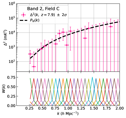
Figure 20: Here we show in greater detail the most sensitive 2$\sigma$ upper limit on the 21 cm power spectrum we report, namely 457 mK² at 0.34 $h$Mpc^-1 Band 2 ($z=7.9$), Field C. The information in the top panel is identical to that in Figure 19. We also include the window functions $W(k)$ in the bottom panel, which tell us how each measurement is expected to be a linear combination of the underlying bandpowers. All band window functions peak at the measured $k$ and are relatively narrow, hence the relatively narrow horizontal errors bars which are interpolated from the window functions to span the 16th to the 84th percentile.

The window function matrix $\mathbf{W}$, defined in Equation 9 and propagated to the spherical power spectra, tells us the extent to which different bandpower measurements are expected to be the linear combination of the true bandpowers across $k$ modes. Each row—shown as a different colored line in the bottom row of Figure 20—sums to 1 by definition. The fact that each row is peaked along the diagonal of the matrix means dominant contribution to each measurement is in fact the $k$ mode at which the measurement is reported.

As discussed in Section 3.3.4, these window functions more precisely take into account the delay approximation than the more simpler calculation used in H22a. While they may look similar to the window functions presented in H22a because of the linear scale used in the figure, there are as many as three orders of magnitude of difference in the amplitude of the tails, with the delay approximation leading to a large underestimate (Gorce et al. 2022). This is particularly important if the true 21 cm power spectrum has features in $k$ space or deviates substantially from a roughly flat power law in $\Delta^{2}(k)$, though that is not the case in most “vanilla” models of reionization.

6 Statistical Tests of the Power Spectrum Upper Limits

In this section we report on a series of statistical tests designed to build confidence in our upper limits. Our goal is to test the self-consistency of our results by showing that they either integrate down like noise or are inconsistent with noise in ways that are well understood. Likewise, we split our data set in various ways to look for signs of possible residual systematic effects. By repeating key tests from H22a, we can help ensure that no new failure modes have cropped up.

6.1 Noise Integration Tests at High Delay

As in H22a, we performed a series of noise integration tests to determine whether bandpowers outside the wedge region are consistent with being noise-dominated. By cumulatively averaging the samples that went into the fully-averaged power spectra shown in Figure 19, we are able to test whether the samples average together as would be expected for bandpowers formed from uncorrelated (white) random noise, or whether an additional correlated or non-random signal, such as a source of systematic contamination, may be present.

Our first test is to simply integrate all bandpowers above a fixed $k$. Following H22a, we randomly draw 300,000 pure-noise realizations of the bandpowers using the error covariance matrix propagated through our various averaging steps and used to set the error bars on our power spectra. We then compute the fraction of noise realizations that are larger than the data, which is by definition the $p$-value of the measurement if the null hypothesis is that measured values are drawn from the noise covariance and have mean zero. In Table 5, we show the results of this test for both the real and imaginary parts of both bands’ and all fields’ power spectra.

Table 5: Statistical $p$-values, testing the consistency of the real and imaginary components of the spherical $\Delta^{2}(k)$ with noise over different overlapping ranges of $k$. At high $k$, most measurements are consistent with noise. At low $k$, we do see decisive evidence for residual systematics (values when $p<0.01$, in bold)—mostly foregrounds and perhaps also crosstalk, especially in Band 1. We do not quote numbers below $p<0.001$, since we cannot precisely calculate such low $p$-values with our 300,000 random draws.

	$p$-value
Data Selection	$k\geq 0.2$	$k\geq 0.5$	$k\geq 1.0$
Re[$\Delta^{2}$], Band 1, Field A	$<$0.001	0.378	0.464
Im[$\Delta^{2}$], Band 1, Field A	$<$0.001	0.052	0.089
Re[$\Delta^{2}$], Band 1, Field B	$<$0.001	0.015	0.730
Im[$\Delta^{2}$], Band 1, Field B	0.773	0.633	0.844
Re[$\Delta^{2}$], Band 1, Field C	$<$0.001	0.016	0.050
Im[$\Delta^{2}$], Band 1, Field C	0.182	0.790	0.859
Re[$\Delta^{2}$], Band 1, Field D	$<$0.001	0.015	0.024
Im[$\Delta^{2}$], Band 1, Field D	0.810	0.925	0.686
Re[$\Delta^{2}$], Band 1, Field E	$<$0.001	0.745	0.939
Im[$\Delta^{2}$], Band 1, Field E	0.343	0.686	0.506
Re[$\Delta^{2}$], Band 2, Field A	$<$0.001	0.182	0.124
Im[$\Delta^{2}$], Band 2, Field A	0.262	0.320	0.144
Re[$\Delta^{2}$], Band 2, Field B	0.077	0.385	0.654
Im[$\Delta^{2}$], Band 2, Field B	0.499	0.398	0.356
Re[$\Delta^{2}$], Band 2, Field C	0.198	0.214	0.314
Im[$\Delta^{2}$], Band 2, Field C	0.041	0.120	0.095
Re[$\Delta^{2}$], Band 2, Field D	0.007	0.767	0.937
Im[$\Delta^{2}$], Band 2, Field D	0.100	0.116	0.366
Re[$\Delta^{2}$], Band 2, Field E	0.006	0.276	0.724
Im[$\Delta^{2}$], Band 2, Field E	0.383	0.714	0.819

In general, we find our imaginary power spectra consistent with noise across $k$, as expected. The one exception is in Field A for Band 1, where we are likely seeing noise-foreground cross terms dominating the imaginary power spectrum. Our real power spectra are another matter. We see strong evidence for inconsistency with noise at low $k$, which is expected given the foreground leakage just outside the wedge buffer in both cylindrical power spectra (Figure 17 and Figure 18) and at low $k$ in spherical power spectra (Figure 19). In Band 1, we also see more marginal evidence for inconsistency with noise even after $k<0.5\,h{\rm Mpc}^{-1}$ is excluded. This is likely attributable to residual crosstalk, which appears in our final power spectra at the few-$\sigma$ level.

While the $p$-values are a useful test of the null hypothesis on the final power, a lot can be obscured by collapsing an entire power spectrum to just a few numbers. To further probe the consistency of our results with noise, especially at high delay, we perform two additional tests. The first assesses how baselines integrate down within a redundant group. In Figure 21 we examine how a single delay mode at $\tau\approx\pm 3000$ ns integrates down as more baselines are added to the cumulative average.

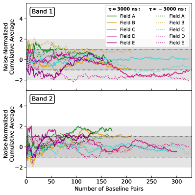
Figure 21: Cumulative average of the (crosstalk-subtracted) delay power spectrum for a single redundant baseline group (29 m east-west) as a function of the number of baseline pairs, for our two frequency bands and five fields. Only the results for single bandpowers at $\tau\approx\pm 3000$ ns are shown here, corresponding to $k\approx 1.48$ $h\,{\rm Mpc}^{-1}$ (Band 1) and $k\approx 1.68$ $h\,{\rm Mpc}^{-1}$ (Band 2). This is well above the crosstalk contaminated delay range. Solid lines denote positive delays, dotted denote negative delays, and an incoherent time average within each field has been performed for each baseline pair before the cumulative average. Different amounts of flagging apply to each band, field, and bandpower, hence the different lengths of the lines. The cumulative average is normalized by the expected noise variance, calculated from the mean noise power over each field/band; see the text for more details. The gray bands show regions of 1$\sigma$ and 2$\sigma$ corresponding to where the cumulatively-averaged power spectra of white noise with the same (inhomogeneous) noise variance as the data, $P_{N}$, would be expected to fall 68% and 95% of the time. We see no strong evidence for any violation of the null hypothesis that these baseline groups average down like noise at this delay.

We use our most sensitive redundant group—the 29 m east-west baseline. We normalize the cumulative average by the expected variance of that cumulative average derived from $P_{N}$. We show 1$\sigma$ and 2$\sigma$ regions where we expect 68% and 95% of pure noise realizations to fall in gray. We have validated this calculation with a set of 100 white noise-only simulations that have been passed through the same flagging, weighting, and power spectrum estimation steps as the real data. The simulations are constructed to have noise variance that depends on time, frequency, and baseline in the same way as the data, according to our empirical estimates of the noise power spectrum $P_{N}$.

The overall conclusion from Figure 21 is that there are no strong deviations from the expected noise-like behavior for any band or field in our data set at $|\tau|\approx 3000$ ns, according to this statistic. Band 1, Field D has the most substantial deviations, but these remain largely within the 95% region. Band 2, Field A also approaches the edge of the 95% region. Bands 1 and 2 of Field C have averages that are more consistently close to zero than for any of the others, though this is not necessarily a statistically significant anomaly.

Another similar test is shown in Figure 22 where we examine the same baseline group, but average over baselines in the group and over a wider range of delays ($\pm$2000–4000 ns) to look for evidence of LST-dependent systematics.

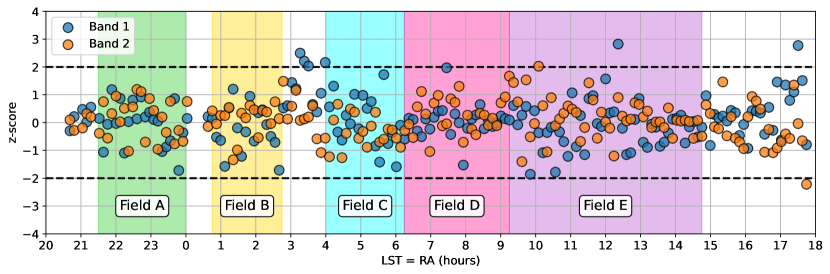
Figure 22: We examine our data for LST-dependent systematics by computing the $z$-score of the bandpowers averaged over a delay range of 2000–4000 ns for the 29 m east-west baseline group. The expected standard deviation at each LST is estimated by recomputing the bandpower average for 100 noise realizations matched to the thermal noise in the data. Dashed horizontal lines mark a $z$-score of 2, showing very few significant outlier in the data across the LST range.

We compare each average to the distribution of 100 noise realizations which are drawn from $P_{N}$ and reflect the real data’s sampling and cuts. In the fields of interest, we see little evidence for significant outliers, indicating that there is no strongly LST-dependent high-delay systematic affecting our results for this baseline group. Outside our fields, we do see some large outliers from Fornax A and the Galactic center which might be concerning in the future if they appear elsewhere in HERA data as we integrate deeper.

6.2 Testing Systematics Mitigation

Though we have taken several steps to mitigate the effect of crosstalk—including subtracting it from our visibilities and cutting baselines that exhibit substantial residuals (see Section 3.2.4)—it is useful to understand how those choices may have affected the distribution of bandpowers. In H22a we performed a one-sample Kolmogorov-Smirnov (KS) test comparing the cumulative distribution function (CDF) of power spectra over 0.4 hours of LST to a validated analytic noise model.

Here we iterate slightly on that test with a two-sample KS test comparing the CDF of measured bandpowers for the redundantly-averaged 29 m east-west baseline group to that of the same 100 noise realizations as in our $z$-score test above. Each CDF is computed over LSTs in Field C and over a series of 200 ns-wide delay bins (except the first bin, which spans 0–500 ns). In Figure 23, we show the results of that work for both bands and for data with (dashed lines) and without cross-talk subtraction (solid lines).

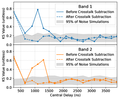
Figure 23: Here we quantify the impact of crosstalk subtraction with a two-sample Kolmogorov-Smirnov computed for various ranges of delays for 29 m east-west baseline group. The KS test is performed by computing the cumulative distribution function of the bandpowers over different ranges of delays and LSTs in Field C and comparing it to the CDF of simulated noise. Grey regions mark $2\sigma$ confidence intervals for the delay range to be consistent with thermal noise expectations. Delay ranges are 200 ns wide with the exception of the point, which encompasses delay ranges of 0–500 ns. The upper and lower panels show the KS tests for Band 1 and Band 2 respectively. KS values after crosstalk subtraction, shown in dashed lines, are consistent with thermal noise expectations outside 500 ns.

To infer the expected range of distances between CDFs, we also compute a distribution of two-sample KS statistics for each delay ranges by comparing many pairs of independent noise realizations. We show the 2$\sigma$ range of that distribution in the gray band of Figure 23. We can see that while the distribution of bandpowers was highly inconsistent with noise before crosstalk subtraction, afterwards they are consistent beyond 500 ns for this baseline group.

6.3 Jackknife Tests Across Epochs

In order to check the consistency of the epochs (defined in Section 2.1) at the bandpower level and thus justify (post hoc) the decision to combine them to arrive at our final limits, it is useful to begin by looking at single-epoch power spectra. These are formed by simply going straight from crosstalk subtraction to forming pseudo-Stokes I and coherently averaging. In Figure 24, we show one such power spectrum from Band 2, Field C—our deepest limit—and compare measurements and vertical error bars from individual epochs to the full data set.

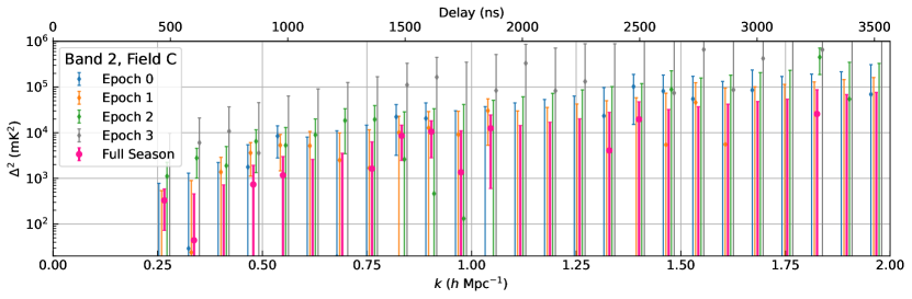
Figure 24: Here we show power spectra estimated for each epoch individually, as well as those for the full data set, for Band 2, Field C. Each individual epoch has higher noise levels than the full season combined, especially Epoch 3 which only partially overlaps with Field C. Vertical error bars are 2$\sigma$. For clarity, horizontal error bars have been omitted and individual epochs’ power spectra are plotted a slightly displaced $k$s. Whether there is clear evidence for any particular epoch being a strong outlier, here or for other bands or fields, is a question we seek to answer in Figure 25.

The full data set’s power spectrum (which is identical to that in Figure 20), is generally lower than any individual epoch. Since most individual epochs are consistent with noise, this is not too surprising. Since the epochs are binned together with weights proportional to the number of visibility samples, it is not trivial to look at this figure and read off the impact of each epoch on any given $k$ mode. Therefore, while there are no obvious inconsistencies visible here, it behooves us to approach the question more quantitatively.

We answer that question by performing a Bayesian jackknife test across epochs. This test is described in detail in Wilensky et al. (2022); we summarize our specific implementation of it here. For each band, field, and spherically-averaged $k$-mode, we consider $2^{N}$ hypothetical models for the $N\leq 4$ epochs that contribute to the particular band and field’s power spectrum at the specified $k$-mode (Epoch 0, for example, does not contain any observations in Field E). In each hypothetical model, we propose that a bandpower is either unbiased—i.e. consistent with zero-mean noise—or strongly biased—i.e. consistent with measuring a signal—by an unspecified amount within a relatively constrained prior range. To compute the posterior for each model, we marginalize over a multivariate Gaussian bias prior that is centered at $6\sigma_{i}$ with a width of $\sigma_{i}$ in each direction, where $\sigma_{i}$ is the square root of the estimated variance for the $i$th bandpower. This is intended to represent a strong but not excessive bias with an a priori SNR in the 4–8 range. We then use a series of Bayesian model comparisons to identify which epoch(s) is most likely to be biased for any given bandpower.

Figure 25 shows the results of this test for each band, field, and $k$ mode.

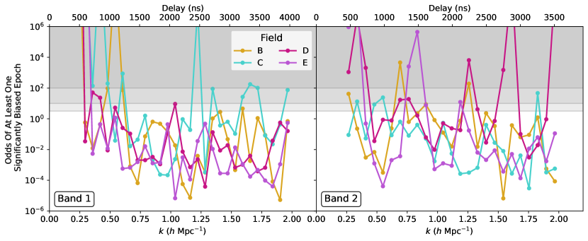
Figure 25: Here we show the odds of at least one epoch being significantly biased, as a function of $k$ for each band and field, as determined by our a Bayesian jackknife test. We observe that for most bands, fields, and $k$ modes, there is only occasionally “strong” evidence (odds $>10^{1}$; medium gray region) or “decisive” (odds $>10^{2}$; dark grey) for a significantly biased epoch, using the terminology of Kass & Raftery (1995). The majority of points fall beneath the region of “substantial” evidence (odds $>3.2$; light gray) as well. Band 1, Field C shows consistent evidence for possessing a significantly biased epoch. Examination of the posterior over bias configurations (see Wilensky et al. 2022) suggests that Epoch 1 is most likely to be biased for a number of $k$ modes in Band 1, Field C. The biases observed in Band 2, Fields D and E are less clearly attributable to a single epoch. Notably, Band 2, Field C (see Figure 24) shows only mild or occasionally strong evidence for the presence of a bias.

To calculate the inferred odds of there being at least one significantly biased epoch— albeit only when the large biases reflected by the alternate hypotheses are considered—we have evaluated the posterior probability of each bias configuration, summed those in which at least one bias is present, and divided by the posterior probability of the null hypothesis that no biases were present. We use a flat prior for the bias configurations. We generally find that for the majority of bands and fields, most spherically-averaged Fourier modes are more consistent with pure noise than a scenario with an epoch-dependent bias, particularly for higher-$k$ modes (see the caption of Figure 25 for a discussion of fields/epochs that potentially deviate from the null hypothesis). Since crosstalk subtraction is performed on a per-epoch basis, it is likely that residual crosstalk is a major source of bias that varies from epoch to epoch. This majority-null result justifies the decision to average the epochs together into one final power spectrum for each band and field.

This is not to say that we strongly suspect there is no underlying signal due to residual systematics or one of cosmological origin. Since only large biases are considered in the alternate hypotheses, our conclusion is that if biases are present, then they are sufficiently small to be difficult to distinguish from the expected statistical fluctuations in the bandpowers. Indeed, if we marginalize over bias priors centered at smaller biases (e.g. less than $\sigma_{i}$), the posterior probability of the bias configurations is more evenly diffused over the hypotheses, demonstrating a lack of certainty that arises from an inability to finely distinguish weak bias configurations with so few data.

7 Constraints on the Astrophysics of Reionization and the Cosmic Dawn

Having established our new upper limits on the 21 cm power spectrum at both $z=7.9$ and $z=10.4$, we now turn to their astrophysical implications. Just as much of this work so far has been the application of the techniques developed in H22a and its supporting papers, in this section we directly apply the techniques laid out in H22b to our updated power spectra. We begin by explaining how we compute model likelihoods in order to perform astrophysical inference in a Bayesian framework (Section 7.1). In Section 7.2, we then briefly survey the four techniques employed in H22b and compare their updated constraints on the ratio of the average spin temperature of the IGM to the temperature of the radio background, $\overline{T}_{S}/T_{\rm rad}$. After giving some background detail on the two simplest models in Section 7.3, we proceed with a more detailed report of updated techniques and results from both 21cmMC (Section 7.4) and from models with an extra radio background generated by galaxies (Section 7.5). Finally, we conclude in Section 7.6 with a more comprehensive comparison of our models and the significance of their results in the broader context of 21 cm cosmology.

7.1 Evaluating Model Likelihoods

To interpret the power spectra and upper limits reported in H22a, all four techniques examined in H22b employ the same statistical approach to evaluating the posterior probability of model parameters in a Bayesian framework. Each theoretical model $\mathcal{M}$ with a set of parameters $\bm{\theta}$ compares the data $\mathbf{d}$ to modeled power spectra $\mathbf{m}(\bm{\theta})$ convolved with the window function $\mathbf{W}$. We write this difference as $\mathbf{t}\equiv\mathbf{d}-\mathbf{Wm}(\bm{\theta})$. We next assume that each measurement is due to some unknown combination of 21 cm signal, noise, and systematics. Further we assume that systematics (typically residual foregrounds and crosstalk) can only add power. These assumptions are only appropriate when claiming upper limits on the 21 cm power spectrum, as we do in this work. To claim a detection, one would have to impose additional constraints on the relative contribution of systematics to the measurement. To do that credibly, one likely needs high SNR detections at multiple $k$ modes, redshifts, and fields, which can be subjected to rigorous jackknives and other statistical tests for internal consistency, along with a theoretical framework able to match the data well.

Marginalizing over systematics, as we show in H22b, yields a posterior probability of the form

$$p(\bm{\theta}|\mathbf{d},\mathcal{M})\propto p(\bm{\theta}|\mathcal{M})\prod_{i}^{N_{d}}\frac{1}{2}\left(1+{\rm erf}\left[\frac{t_{i}}{\sqrt{2}\sigma_{i}}\right]\right)$$ (11)

where the product on the right-hand side is the likelihood. Here $N_{d}$ is the number of data points considered and $\sigma_{i}$ is the standard deviation of $d_{i}$. This result is consistent with similar approaches in the literature (Li et al. 2019; Ghara et al. 2020). In this derivation, we also assumed that measurements have uncorrelated errors. While neighboring measurements in $k$ are in fact quite correlated, we follow H22b and throw out every other measurement in $k$—keeping the absolute lowest limits—to largely eliminate that correlation.

To understand the effect of the form of the likelihood in Equation 11, we calculate it using a power law $\Delta^{2}\propto k^{\alpha}$ over several orders of magnitude in $\Delta^{2}$ evaluated at $k=0.35$ $h$Mpc^-1 in Figure 26.

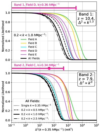
Figure 26: Here we show our marginalized likelihood from Equation 11 for each band and multiple fields and ranges of $k$. In solid colored lines, we show the likelihood for each field independently, but combine all $0.2<k<1.0$ $h$ Mpc^-1 after throwing away every other power spectrum measurement to eliminate correlated errors. To combine multiple $k$ values, we have assumed a power law $\Delta^{2}\propto k^{\alpha}$ where $\alpha=1.3$ at $z=10.4$ and $\alpha=0.0$ at $z=7.9$. In the various black curves, we combine together all fields but use different ranges of $k$ values, including just the $k$ of the best upper limits at $k\approx 0.35$ $h$Mpc^-1. To help provide some intuition for how the upper limits yield these likelihoods, we also show the best upper limit from each band (pink error bars, taken from Figure 19 and rotated 90^∘). It is clear that combining together multiple fields has an effect, especially for Band 1 ($z=10.4$) where Fields C and D contribute roughly equally. Likewise, combining together multiple $k$ modes tightens the constraints significantly, especially at $z=10.4$ where power law is steeper. When evaluating the posterior probability of our various models and parameters, we compare the models to the data at the proper $k$ values.

At $z=10.4$, we use $\alpha=1.3$; at $z=7.9$ we use $\alpha=0.0$. These values of $\alpha$ were derived by interpolating the 21cmMC power spectrum realizations in our posterior without HERA (see Section 7.4.3) at the $k$ values of our two deepest measurements, fitting a power law, and then taking the median $\alpha$ over models that had not yet completely reionized. The flattening of $\Delta^{2}$ with decreasing redshift is a generic consequence of inside-out reionization, which suppresses small-scale power.

The first thing to note is that our likelihoods are essentially flat for $\Delta^{2}$ values much less than the upper limit; the signal could fall anywhere in that range because the systematics could fall anywhere in that range as well. Our results can therefore be heavily impacted by the prior, $p(\bm{\theta}|\mathcal{M})$, and what it considers the smallest viable power spectrum.

Figure 26 also highlights the fact that, in contrast to H22b, our result features fairly comparable limits from multiple fields and $k$ modes. Because our likelihoods are not Gaussian, the results do not scale like $1/\sqrt{N}$ as one might expect. Limits with larger measurements and smaller error bars look different in Equation 11 than measurements with the same $2\sigma$ upper limits but with smaller measured $\Delta^{2}$ and larger error bars. So, while it is not surprising that most of the information in Band 2 comes from Field C, it is interesting and not necessarily intuitive that Fields C and D contribute equal amounts of information in Band 1. Likewise, we can see that just using a single $k$ mode (dotted black lines)—even though it is the single best upper limit and combines together all fields—yields somewhat worse constraints than combining multiple $k$s. The vast majority of the constraining power comes form $k<1$ $h$Mpc^-1 (solid black line). Of course, combining $k$ modes together in this way is only technically correct if we are evaluating the likelihood in Equation 11 for a model with $\Delta^{2}\propto k^{\alpha}$. In general, our model posteriors use all fields and all $k$-values, but compare them to the data at the proper $k$ values.

7.2 Overview of Theoretical Models and their IGM Spin Temperature Constraints

In H22b, we interpreted the results of H22a using a suite of four different theoretical models to infer constraints on the IGM and high-$z$ galaxies:

1. a simple “density-driven” linear bias model, in which the 21 cm fluctuations are assumed to trace the density fluctuations, multiplied by a bias factor that depends on the average thermal and ionization state of the IGM;

2. a phenomenological “reionization-driven” model, which parameterizes the ionized bubble distribution and IGM spin temperature directly without making any explicit assumptions about galaxies (Mirocha et al. 2022);

3. a semi-numeric model of the 21 cm signal, 21cmFAST (Mesinger et al. 2011), along with the inference engine 21cmMC (Greig & Mesinger 2017) that uses it to explore and constrain a range of parameterized galaxy properties (e.g. Park et al. 2019) with multi-wavelength probes; and

4. an independent semi-numeric model that models the galaxies differently and allows for a radio background in excess of the CMB at high redshifts (Reis et al. 2020).

Our models are constructed in two qualitatively different ways. The density-driven and reionization-driven models interpret the 21 cm signal directly as a function of IGM properties. They avoid making explicit assumptions about the sources generating the radiation fields that determine the 21 cm signal (though their priors on IGM properties carry some implicit assumptions), and as such have a lighter implementation. The semi-numeric models, on the other hand, start with a model of galaxy evolution and simulate a cosmological volume in order to predict the 21 cm signal. The latter are significantly more complicated but have the distinct advantage of a parameter set that is rooted in our current understanding of galaxy properties, which allows us to combine 21 cm measurements with other constraints on the galaxy population (such as UV luminosity functions and the X-ray background). The disadvantage of the semi-numeric approach is that the resulting constraints on galaxy physics are only sensible if their parameterization is flexible enough to include all the relevant physics. In H22b we considered two independent semi-numeric models to mitigate this problem.

The key result of H22b, across all these models, was that the IGM must have been heated above the expectation for an adiabatically cooling IGM from recombination to $z=7.9$ at $>$95% credibility. If this heating is interpreted in the conventional way—as the result of X-rays generated by accretion onto black hole remnants of early star formation and then depositing that thermal energy in the IGM—this level of heating suggested that early galaxies were more efficient X-ray emitters than their local counterparts. If an excess radio background were allowed, the observations jointly constrained the efficiencies of radio and X-ray emission from galaxies, also restricting the parameter space of otherwise viable models of these mechanisms during the EoR.

In this work, we apply those same four techniques—with some minor adjustments, as we will discuss below—to our data from both bands. As H22b argued, the easiest point of comparison for the models is the inferred average spin temperature of the neutral IGM, $\overline{T}_{S}$. In Figure 27 we compare the 68% and 95% highest posterior density (HPD) credible interval on $\overline{T}_{S}$ in all four models and show how those constraints have improved since H22b.

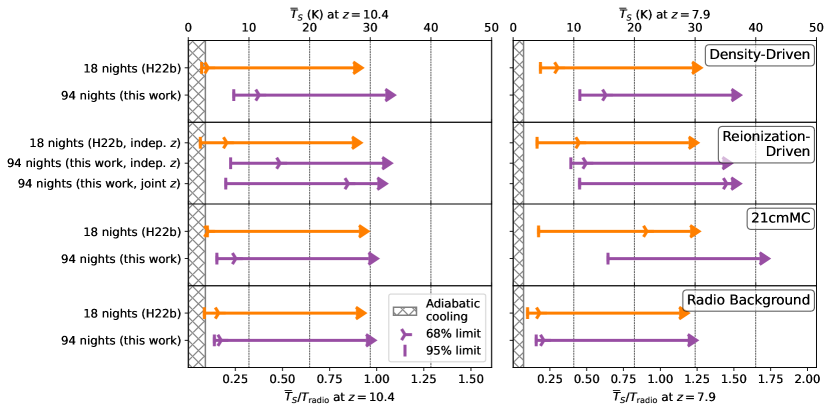
Figure 27: Here we summarize HERA’s constraints on the IGM spin temperature $T_{S}$ and contrast $T_{S}/T_{\rm radio}$ at $z=10.4$ (left) and $z=7.9$ (right). Each row shows the HPD results obtained with a different model for 21-cm fluctuations (described in Section 7). These include a linear bias model with density fluctuations only (top row; see Section 7.3); a phenomenological model that parametrizes the ionized bubble size distribution and assumes an IGM of uniform temperature (second row; also see Section 7.3); 21cmMC, a Bayesian technique for fitting parameters of semi-numeric 21cmFAST simulations (third row; see Section 7.4); and another semi-numerical model that includes a prescription for radio emission generated by galaxies (bottom row; see Section 7.5). In each panel, we compare results obtained in this work with the previous set of upper limits published in H22b, where we only saw evidence for heating above the adiabatic limit (gray hashed region) at $z=7.9$. In this work, we see consistent evidence across all our models for an IGM heated above the adiabatic at $z=10.4$ as well. The more dramatic rise of the $z=7.9$ spin temperature in 21cmMC relative to the other models is driven by the $z=10.4$ constraints combined with independent constraints on galaxy luminosity functions (as we discuss in detail in Section 7.6). Note that for the first three models, $T_{\rm{radio}}=T_{\rm{CMB}}$, which enables a conversion between the top and bottom axes. For the model in the bottom row with an excess radio background, $T_{\rm{radio}}\neq T_{\rm{CMB}}$ in general, and so the $T_{S}$ tick marks along the top axis should be ignored.

The improvements are modest but consequential, especially at $z=10.4$: all four models now independently require the IGM to be heated above the adiabatic cooling limit at $>$95% credibility. The precise values of lower limits vary from model to model, reflecting their different assumptions and approximations. In particular, 21cmMC shows the most dramatic increase in the spin temperature constraint at $z=7.9$, a fact that deserves further examination. As we discuss the specific models and their detailed results throughout this section, we will look to understand what precisely drives these differences. In Section 7.6, we will summarize our takeaways and put these spin temperature constraints in the broader cosmological context.

7.3 Phenomenological Models of the 21 cm Power Spectrum

Before we discuss the detailed results of our more complex techniques for astrophysical inference based on semi-numerical simulations, here we briefly detail the two simpler methods used in H22b to infer constraints on the spin temperature and other IGM properties.

In the first, which we refer to as the “density-driven” model, the 21 cm power spectrum is assumed to follow that of matter, multiplied by a bias parameter squared (as is standard in perturbation theory, see e.g. McQuinn & D’Aloisio 2018; Georgiev et al. 2022; Qin et al. 2022; Sailer et al. 2022 for more complex approaches). Limits on this bias can then be translated into lower bounds on $\overline{T}_{S}/T_{\rm CMB}$ under some assumptions, including redshift-space distortions as a function of the line-of-sight cosine $\mu$, see H22b) and that the IGM properties are roughly homogeneous (as the model ignores ionization and temperature fluctuations beyond adiabatic, see H22b for details). Our limits on the bias $b_{m}$ using 94 nights (and all fields and every other $k$, as discussed above) are $|b_{m}|<60$ mK at $z=7.9$ and $|b_{m}|<160$ mK at $z=10.4$ at 95% credibility, which assuming $x_{\rm HI}=1$ translate into the IGM limits shown in Figure 27 and in Figure 34. Note that these limits are on the absolute value $|b_{m}|$. This is unimportant for cases where $\overline{T}_{S}\ll T_{\rm radio}$, but as the limits tighten we will obtain contours around $\overline{T}_{S}=T_{\rm radio}$ (which yields no 21-cm signal and thus $b_{m}=0$). In fact, the 68% credible limit on the $z=7.9$ bias is $|b_{m}|<30$ mK, which translates into the double-sided region from $\overline{T}_{S}=15$ K to $\overline{T}_{S}=60$ K (assuming $T_{\rm radio}=T_{\rm CMB}$, as is standard).

In the second, which we refer to as the “reionization-driven” model, the IGM is modeled as a two-phase medium, with fully ionized bubbles drawn from a log-normal size distribution and the “bulk” IGM outside bubbles assumed to be of uniform temperature (as described in Mirocha et al. 2022). The advantage of this approach is that it works directly with IGM quantities, which makes it easy to interpret, and avoids making explicit assumptions about galaxies. In its simplest form, it requires four parameters: the volume filling fraction of ionized gas, $Q\equiv(1-x_{\rm HI})$, the IGM spin temperature, $\overline{T}_{S}$, the characteristic bubble size, $R_{b}$, and log-normal dispersion, $\sigma_{b}$. In this work, when jointly fitting both HERA bands, we also use a 7-parameter version of the model in which the ionized fraction and characteristic bubble size are allowed to evolve with redshift as power laws. We require only that $Q$ and $R_{b}$ increase with time, that reionization completes at $z\geq 5.3$, and that all parameters are positive. We perform our Markov Chain Monte Carlo (MCMC) inference using emcee (Foreman-Mackey et al. 2013).

Now, with 94 nights of data, we infer spin temperatures in excess of the adiabatic cooling limit at $z=7.9$ and $10.4$, both for fits that consider each band separately and the joint fit to both bands using a 7-parameter version of the model (see Figure 27). At 95% (68%) credibility we obtain $\overline{T}_{S}>11.0$ (35.2) K at $z=7.9$, and $\overline{T}_{S}>6.2$ (26.4) K at $z=10.4$, when fitting both bands simultaneously. Note that, in this joint fit, lower limits on $\overline{T}_{S}$ grow at $z=7.9$, as expected, but actually slightly decrease at $z=10.4$ (at 95% credibility) relative to the results of single-band fits. This is a result of using an HPD estimate of the credible interval, combined with change in the shape of the $\overline{T}_{S}$ posterior, which goes from being roughly flat as $\overline{T}_{S}\rightarrow 10^{3}\ \rm{K}$ to a more “peaked” distribution, slightly away from the maximal value of $\overline{T}_{S}$. This is consistent with the results of the density-driven model, suggesting that our limits are beginning to disfavor scenarios with saturated $\overline{T}_{S}$ at $z=7.9$.

The differences between these approaches explains some of the differing conclusions in Figure 27. For example, the density-driven model yields higher $\overline{T}_{S}$ limits than the reionization-driven model, because the latter assumes ionization and density are positively correlated. As a result, the IGM must be made colder to compensate for the loss of the densest regions to ionization. We see also in the reionization-driven model the power of jointly fitting multiple bands; the $z=7.9$ limit increases by roughly a factor of 2 in the joint fit because a given temperature at $z=7.9$ is only viable if the temperature evolution is consistent with the $z=10.4$ data.

7.4 Updated Constraints on Reionization and X-ray Heating of the IGM with 21cmMC

21cmFAST (Mesinger et al. 2011; Murray et al. 2020) is a semi-numerical simulator for computing the evolution of the 21 cm signal across cosmic time by assuming that star-forming galaxies, hosted by dark matter halos, drive the cosmic radiation fields that heat and ionize the IGM. It uses empirical scaling relations to assign galaxy properties to dark matter halos based on their halo masses. These include the stellar mass to halo mass ratio, the UV ionizing escape fraction, the star formation rate, and the X-ray luminosity. 21cmFAST simulates reionization using the excursion-set formalism (Furlanetto et al. 2004). It accounts for inhomogeneous recombinations (Sobacchi & Mesinger 2014) and includes a numerical correction for photon conservation (Park et al. 2021).

In Section 5.1 of H22b, we discussed the nine physically-meaningful free parameters that go into the scaling relations describing galaxy properties (also see Park et al. 2019). We adopted either flat linear or logarithmic priors—depending on the parameter’s dynamic range and how it enters into the model—within our 9-dimensional hypercubic parameter space. The ranges on these priors were picked to allow a broad range of physically plausible values while not strongly constraining the parameters most constrained by other high-redshift probes. These include UV luminosity functions (Bouwens et al. 2015, 2016; Oesch et al. 2017) and measurements of the IGM opacities during the EoR such as the Ly-$\alpha$ forest (McGreer et al. 2015; Bosman & Becker 2015; Qin et al. 2021a) and CMB polarization and optical depth (Planck Collaboration 2018; Qin et al. 2020). The Ly-$\alpha$ forest and the CMB’s $\tau$ provide important clues as to the timing and duration of reionization, which then constrain the ionizing escape fraction, given the observed UV luminosity function. We use 21cmMC (Greig & Mesinger 2015, 2017) and its MultiNest sampler (Feroz et al. 2009; Qin et al. 2021b) to perform Bayesian inference in this work. The posterior probability distribution without HERA serves as the starting point for comparing models against HERA data.

One key result from these other high-redshift probes is the strong constraint on the star formation efficiency of dark matter halos at high redshift, which is determined by the UV luminosity functions at $z\sim 6$–8; existing observations constrain both the peak efficiency and show that it declines toward small halo masses (e.g., Tacchella et al. 2013; Mason et al. 2015; Mirocha et al. 2017; Park et al. 2019; Sabti et al. 2022). The version of 21cmFAST used here assumes that this behavior can be extrapolated to higher redshifts and smaller haloes. As a result, the range of galaxy formation models that are allowed by 21cmMC is relatively restricted, and all display a rapid increase in the stellar mass density between the two redshifts measured by HERA. The resulting constraints must be interpreted with this in mind, as more complex galaxy evolution histories (which break the assumed extrapolation by, for example, introducing a new population of sources, see e.g. Muñoz 2019; Qin et al. 2020; Muñoz et al. 2022 for implementations in 21cmFAST) are not included in the prior and are left for future work.

7.4.1 21cmMC Constraints on X-Ray Luminosity

In H22b we explored how adding HERA affected the full posterior parameter covariance. In this work, we focus on the parameter most constrained by HERA, the ratio of the integrated soft-band (${<}2$keV) X-ray luminosity to the star formation rate. Since 21cmFAST assumes that X-ray photons govern the thermal history of the neutral IGM, this $L_{\rm X<2keV}$/SFR parameter essentially describes the heating power of EoR galaxies per unit of star formation. In H22b, we obtained the first observational evidence for an enhanced X-ray luminosity of high-redshift ($z>6$) galaxies, with a 68% HPD credible interval of $L_{\rm X<2keV}/{\rm SFR}\sim 10^{39.9}$–$10^{41.6}$ erg s^-1 ${\rm M}_{\odot}^{-1}$ yr. This disfavors a relationship between star formation and soft X-ray luminosity at or below the one seen in local, metal-enriched galaxies at $>$68% credibility.

As Figure 28 shows, we find that the full season of HERA observing constrains the 95% credible interval on $L_{\rm X<2keV}/{\rm SFR}$ to the range $10^{40.4}$–$10^{41.8}$ erg s^-1 ${\rm M}_{\odot}^{-1}$ yr.

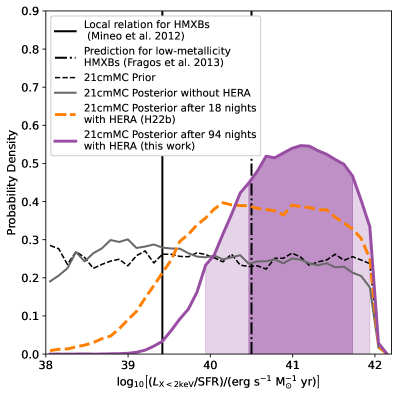
Figure 28: Here we show how our marginalized 21cmMC posterior PDF of the ratio of soft X-ray luminosity to SFR, $L_{\rm X<2keV}$/SFR, tightens with a full season of HERA data. The shaded regions show the 68% and 95% credible intervals of the posterior. Probability densities are plotted per logarithmic interval. Our results are consistent with theoretical expectations for X-rays produced during the cosmic dawn by a population of low-metallicity high-mass X-ray binaries (HMXB) (Fragos et al. 2013), likely a more representative model of the first galaxies (dash-dotted black vertical line). Compared to H22b (orange dashed line), our result’s 99% credible interval excludes models where the local relation for X-ray efficiency (solid black vertical line; Mineo et al. 2012) continues to hold at high redshift.

This result assumes as a prior that $L_{\rm X<2keV}/{\rm SFR}<10^{42}$ erg s^-1 ${\rm M}_{\odot}^{-1}$ yr, beyond which X-rays reionize the universe too quickly (Mesinger et al. 2013). More than 99% of the 21cmMC posterior volume excludes the possibility of the local relation for HMXBs (Mineo et al. 2012) continuing to hold at high redshift. It is consistent, however, with models of extremely low-metallicity galaxies, where high mass stars have less mass-loss from line-driven winds than their solar-metallicity counterparts (Fragos et al. 2013).

7.4.2 21cmMC Constraints on the IGM’s Thermal History

Our constraints on the soft X-ray efficiency are themselves a consequence of our ability to use our upper limits to exclude a range of scenarios with low levels of IGM heating. In Figure 29 we show our updated marginalized posteriors on the predicted average IGM temperatures—both the spin temperature, $\overline{T}_{S}$, and the kinetic temperature, $\overline{T}_{K}$—along with results from H22b for comparison.

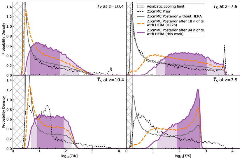
Figure 29: Here we show marginalized 1D PDFs from 21cmMC per logarithmic interval in the kinetic temperature (top row) and spin temperature (bottom row), averaged over the neutral IGM, at both $z=10.4$ (left column) and $z=7.9$ (right column). We compare the prior on these quantities to the posterior from H22b data (orange dashed) and the posterior after a full season (purple, with 68% and 95% credible intervals shaded). We also show our prior (black dashed) and the posterior after including non-HERA astrophysical constraints on reionization (gray). The averaging is performed over neutral cells with $x_{\rm HI}>0.95$; for models completely reionized at $z=7.9$, we take the average temperature from the last time-step with neutral cells. The hashed region indicates temperatures below the adiabatic cooling limit. Our observations rule out an unheated IGM at $>$99% credibility at both $z=10.4$ and $z=7.9$, placing new constraints on the population of X-ray emitting compact objects during the cosmic dawn.

As demonstrated in H22b, current EoR constraints from Planck and quasar spectra already disfavor a large number of models in the prior volume which predict either highly ionized IGM at $z\geq 10.4$ or completely neutral one at $z\leq 10.4$. These constraints also have a slight impact on the average IGM temperature, excluding models with high $\overline{T}_{\rm K}$ or $\overline{T}_{\rm S}$ at these redshifts. However, because a decently-sized fraction of parameter space with an unheated IGM at these redshifts is not ruled by these probes, and since 21cmMC cannot produce spin temperatures below the adiabatic limit, our posterior without HERA shows a pileup of probability right around that limit.

When we incorporate the HERA limits, a significant range of models with low IGM temperatures can be further excluded. We showed in H22b how HERA observations substantially improve our understanding of the neutral IGM at $z=7.9$. However, there was still a small fraction of the total posterior with low values of $\overline{T}_{\rm S}$, so H22b could not completely rule out an unheated IGM the observed redshifts. With the improved limits presented in this work, we now find that an unheated IGM is disfavored at greater than 99% credibility at both $z=10.4$ and 7.9. The new HPD 95% credible intervals on the spin and kinetic temperatures are $4.7$ ${\rm K}<\overline{T}_{S}<171.2$ K and $3.2$ ${\rm K}<\overline{T}_{K}<313.2$ K at $z=10.4$ and $15.6$ ${\rm K}<\overline{T}_{S}<656.7$ K and $13.0$ ${\rm K}<\overline{T}_{K}<4768$ K at $z=7.9$.

Since the 21 cm brightness temperature is proportional to $(1-T_{\text{CMB}}/T_{\text{S}})$, any model where $T_{\text{S}}<0.5T_{\text{CMB}}$ will show an enhanced power spectrum amplitude relative to one where $T_{\text{S}}\gg T_{\text{CMB}}$. Since the CMB is 24.3 K at $z=7.9$, our results rule out the range of cold reionization scenarios with enhanced power spectra at $z=7.9$ with greater than 95% credibility. While we cannot definitively rule out any power spectrum enhancement due to a cold IGM $z=10.4$, we have ruled out the large swath of parameter space that produces the largest power spectra.

Figure 29 brings into sharper relief the question raised by Figure 27 of why the 21cmMC results show such a large change in $\overline{T}_{S}$. Once we reach the regime where $\overline{T}_{S}>T_{\rm CMB}$, large increases in spin temperature have only a modest impact on the power spectrum. It follows then that the updated power spectrum limits at $z=7.9$ are not primarily driving the spin temperature constraint at $z=7.9$. Just as in the reionization-driven phenomenological model where jointly fitting the two redshifts produced tighter $\overline{T}_{S}$ constraints, the combination of our two redshift bands is crucial. In particular, the star formation histories inferred by 21cmMC from UV luminosity functions (in which the stellar mass density increases significantly from $z=10.4$ to $z=7.9$) causes substantial IGM heating between the two bands. Thus the modest heating demanded by HERA at $z=10.4$ translates to a strong inference about the temperature at the later times. We will see quite a similar effect when we examine the inferred power spectrum posteriors in Figure 31.

7.4.3 21cmMC Derived Constraints on the 21 cm Power Spectrum

Because we have ruled out very large negative 21 cm brightness temperatures arising from cold reionization, we can significantly constrain the range of possible values of the 21 cm power spectrum in our model. Figure 30 shows the inferred 68% and 95% posterior equal-tailed credible intervals on the power spectrum at redshifts 12, 10, 8 and 6 after incorporating results of a full season of HERA observation.

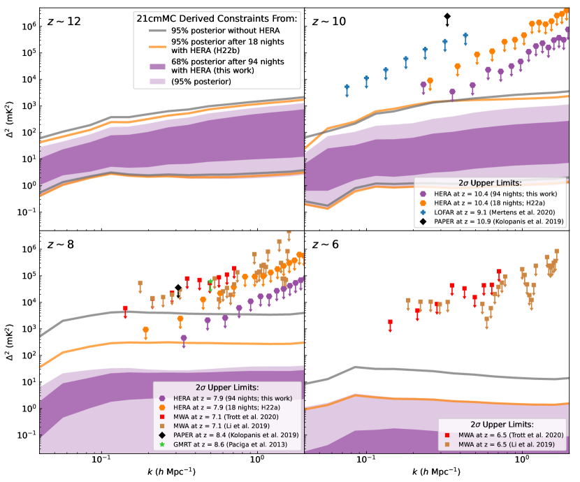
Figure 30: The new upper limits on the 21 cm power spectrum presented here further constrain the possible range of derived power spectra in our 21cmMC posteriors. Here we show the 68% and 95% equal-tailed credible intervals for the inferred power spectra at redshifts 12, 10, 8, and 6, after a full season of HERA (purple). We also show 95% credible intervals after 18 nights of HERA (orange, reproduced from H22b) and without HERA (gray). We also include the HERA $2\sigma$ limits from H22a and this work that most strongly constrain the likelihood, namely the single deepest limit over all fields at each $k$. When evaluating likelihoods, data is compared to models using all fields and $k$, which can make a big difference (see Section 7.1). Note that, due to the form of the likelihood in Equation 11, which depends on both our measurements and our error bars, models with power spectra just below our limits are more disfavored than models with power spectra well below them. To better understand how the shapes of these likelihoods were updated at $z\sim 10$ and $z\sim 8$ and why the contours are often surprisingly far from the deepest limits, see the full posteriors at the $k$ values of our deepest limits in Figure 31. Following H22b, we use every other $k$ to avoid unmodeled correlations between measurements at different $k$ values. For context, we also show the most competitive $2\sigma$ limits from other telescopes at similar redshifts, including GMRT (Paciga et al. 2013), PAPER (Kolopanis et al. 2019), MWA (Li et al. 2019; Trott et al. 2020), and LOFAR (Mertens et al. 2020).

One can think of these contours as the testable—and therefore falsifiable—predictions of 21cmMC given the HERA data, the other astrophysical constraints, and the assumptions of the model. In Figure 30, we also show the 95% equal-tailed credible interval from H22b and from our posterior without HERA. Upper limits from H22a and this work as well as a number of other previously published measurements from GMRT (Paciga et al. 2013), PAPER (Kolopanis et al. 2019), MWA (Li et al. 2019; Trott et al. 2020), and LOFAR (Mertens et al. 2020) are also presented in Figure 30.

It is evident that the HERA limits have been significantly improved since H22a and that this work represents our best constraint so far on the neutral IGM during the EoR. As a result, the posterior distribution of 21 cm power spectra in our model has also become much tighter, which is consistent with our exclusion of an unheated IGM at these redshifts. That said, one might wonder why the 95% posteriors are well below our 2$\sigma$ power spectrum upper limits in Figure 30. The reason is threefold. First, recall that our likelihood model is not Gaussian; it is an error function that asymptotes to a flat probability at small model $\Delta^{2}$ (Equation 11). As Figure 26 shows, power spectra just below our limits are far less likely than power spectra well below them. This concentrates posterior probability at lower power spectrum values. The effect is especially important when multiple fields and $k$ modes contribute significantly to the likelihood, instead of the two measurements from a single field that dominated the results in H22b.

The second reason is that, as already discussed, our inference is heavily informed by other high-redshift observations and the galaxy model assumed by 21cmFAST. This is particularly relevant in the context of the third reason, which is the influence of constraints from the two bands on each other. To better understand the impact of the model, we show in the top row of Figure 31 the prior and full posterior probability distributions from the three inferences, i.e. without HERA and with HERA after 18 (H22b) and 94 nights (this work).

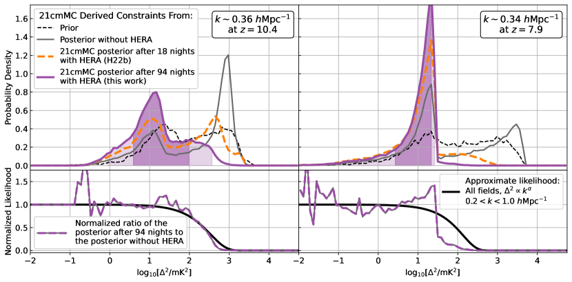
Figure 31: Here we show the full 21cmMC derived prior and posterior PDFs per logarithmic interval in $\Delta^{2}$ at the redshifts and $k$ modes roughly corresponding to our best upper limits (top row). Just as in Figure 29, we show our priori and three posteriors: one with other astrophysics constrains but no HERA (black), one from H22b (orange dashed), and one from this work (purple, with 68% and 95% equal-tailed credible intervals shaded). In the bottom row, we show the ratio of this work’s 21cmMC posterior to the posterior without HERA data. After renormalizing, this ratio is effectively the likelihood that went into the Bayesian update. We compare those effective likelihoods to those calculated in Figure 26 using all fields and all $0.2<k<1.0$ $h$Mpc^-1. It is clear that the update at $z=10.4$ is largely (though not entirely) attributable to the measures at $z=10.4$. However, the update at $z=7.9$ is sharper, indicating that much of the information about the inferred $\Delta^{2}$ comes from ruling out models with inefficient X-ray heating of the IGM, which are better constrained by the $z=10.4$ measurement despite the larger upper limit on $\Delta^{2}$. This in turn helps us understand this work’s 95% contours in Figure 30 relative to H22b, especially at $z=7.9$. Because we have eliminated a broad range of cold reionization scenarios—the right-hand peaks in the pre-HERA posteriors—the 21cmMC posteriors have shifted substantially toward the peaks associated with hot reionization.

We only show the distributions at the $k$ values of our deepest limits, roughly 0.35 $h$Mpc^-1. First consider the PDF without incorporating HERA. It has two clear peaks: the one at smaller $\Delta^{2}$ corresponds to models with $\overline{T}_{S}\gg T_{\rm CMB}$ (with abundant X-ray heating) while the other is mostly “cold reionization” with little heating. In between, there is a valley in the distribution because one must fine-tune the heating and ionization to get a signal between these two extremes, which is comparatively unlikely given our priors and the other high-redshift constraints.

The H22b results ruled out the extreme end of the cold reionization peak $z=7.9$, but at $z=10.4$ much of that stronger peak was still viable. With our new limits, an IGM near the adiabatic limit is essentially excluded at $z=10.4$, which clearly favors models with considerable X-ray heating. Because that heating is assumed by the models to continue through $z=7.9$ (when the stellar mass density, and hence density of X-ray sources, has increased by a factor of a few), the higher-redshift measurement helps to constrain the lower-redshift one as well. In particular, it eliminates the last little tail of large amplitude power spectra in the posterior, which is why the 95% contour moves so much between H22b and this work in Figure 30, though the 68% contour (not shown here for H22b) does not change very much.

As further evidence for the impact of the $z=10.4$ measurements on the $z=7.9$ posterior, we show two additional sets of curves in the bottom row of Figure 31. The first are the ratios of the posterior after 94 nights with HERA to the pre-HERA posterior. The second are the likelihoods that we get from Equation 11 by combining together measurements from all fields and $k$ modes from $0.2<k<1.0$ $h$Mpc^-1 (dropping every other $k$, as discussed in Section 7.1). The likelihoods are evaluated assuming power law $\Delta^{2}\propto k^{1.3}$ at $z=10.4$ and $\Delta^{2}\propto k^{0.0}$ at $z=7.9$ (see Section 7.1 for details). Both curves are normalized to plateau at 1. Since the pre-HERA posterior is treated as the prior for the post-HERA inference, we should expect this ratio to match the likelihood by Bayes’ theorem. It should be noted that using a power-law power spectrum is only an approximation. To understand the precise disagreements between between the likelihood and the ratio of the posteriors, we would have to account for the detailed dependence of $\Delta^{2}$ on $k$, the ways in which the $z=7.9$ measurement constrains the $z=10.4$ posterior (and not just vice versa), and sampling noise.

With those caveats the match looks reasonable at $z=10.4$, but not nearly as good at $z=7.9$. It follows then that the inferred constraints on both $\overline{T}_{S}$ and $\Delta^{2}$ at $z=7.9$ are driven externally to the data at $z=7.9$, which is all that goes into the black likelihood curve. Therefore, the $z=7.9$ results must be a consequence of the $z=10.4$ limits and the way 21cmFAST models the evolution the X-ray luminosity by tying it to star formation and then constraining that star formation rate with other probes, most notably the UV luminosity function. In Section 7.6, we will return to the question of the impact of the specific modeling choices of 21cmMC and how they compare to the other three techniques.

7.5 Updated Constraints on Astrophysical Models with Excess Radio Background

In H22b, we reported parameter constraints on an alternate semi-numerical model that allows for a significant excess radio background. EoR scenarios with high levels of radio background at rest-frame 21 cm wavelengths can potentially produce strong 21 cm absorption signals, since the brightness temperature is proportional to $(1-T_{\text{radio}}/T_{\text{S}})$ (Feng & Holder 2018). We know there exists today a radio background well in excess of the CMB from observations with ARCADE 2 (Fixsen et al. 2011; Seiffert et al. 2011) and the LWA (Dowell & Taylor 2018). It has been theorized that if this excess is sourced by a population of unresolved high-redshift, potentially exotic sources (Ewall-Wice et al. 2018; Fraser et al. 2018; Jana et al. 2019; Pospelov et al. 2018; Brandenberger et al. 2019; Thériault et al. 2021), it could explain the anomalously strong absorption signal seen by EDGES (Bowman et al. 2018). Such explanations are not without difficulty; they would have to feature sources far stronger than what would be expected from local observations (Ewall-Wice et al. 2018; Mirocha & Furlanetto 2019; Mebane et al. 2020; Ewall-Wice et al. 2020) and would need to include rapid X-ray heating at $16\gtrsim z\gtrsim 14$ to explain the high-frequency side of the EDGES trough (e.g. Mittal & Kulkarni 2022).

Since a radio background can also increase the amplitude of 21 cm fluctuations (Ewall-Wice et al. 2014; Fialkov & Barkana 2019; Reis et al. 2020), limits from HERA can constrain astrophysical parameters describing models with excess radio background. In H22b, we used a semi-numerical simulation (Visbal et al. 2012; Fialkov et al. 2014; Fialkov & Barkana 2019; Cohen et al. 2020; Reis et al. 2020, 2021) in which the key radiation fields are all driven by the cosmic star formation rate. This is set (in part) by the star formation efficiency $f_{\rm*}$ with which collapsed gas in halos turns into stars, and the circular velocity $V_{c}$ which determines the minimum mass for star forming halos. Just as in H22b, the efficiencies of X-ray and radio background luminosity relative to the star formation rate are parameterized by $f_{X}$ and $f_{r}$, and reionization is parameterized by the CMB optical depth $\tau$. For more details on the implementation of the model and its parameterization, see Section 8 of H22b.

There are a few differences between the precise inference procedure used here and the one used in H22b. More parameters are now allowed to vary rather than fixing them to specific values. Most significantly, we no longer limit ourselves to the X-ray spectral energy distribution (SED) of X-ray binaries (Fragos et al. 2013; Fialkov et al. 2014) and instead parameterize the SED by a power law spectral index $\alpha_{X}$ (either 1.0, 1.3, or 1.5) and a minimum frequency cutoff $\nu_{\rm min}$ which we vary from 0.1 to 3 keV with log-uniform prior. Additionally, we no longer fix the mean free path to $R_{\rm mfp}=40$ cMpc but vary it between 10 and 70 cMpc. The new parameterization of the X-Ray SED implies that more varieties of X-ray heating are captured. For the same value of $f_{X}$, a softer SED (with a larger number of low-energy photons, e.g. lower $\nu_{\rm min}$) leads to a more efficient heating with shorter X-ray mean free path, while a harder SED (lower number of low-energy photons, e.g. higher values of $\nu_{\rm min}$) results in less heating with a larger fraction of photons remaining unabsorbed.

Another improvement over the analysis performed in H22b is the application of more accurate emulators. Our new emulator, based on the GLOBALEMU formalism (Bevins et al. 2021) and implemented using scikit-learn (Pedregosa et al. 2011), uses a more general neural network reaching an accuracy of $\begin{subarray}{c}+11\%\\ -7\%\end{subarray}$ (at 68% confidence) at $z=7.9$ and $k=\text{0.34\,$h$Mpc${}^{-1}$}$. Additionally, instead of an MCMC, we now use nested sampling with PolyChord (Handley et al. 2015a, b).

The updated analysis and the improved HERA upper limit together result in tightened constraints, two of which are of particular interest. The biggest impact is on the X-ray efficiency $f_{X}$, which is consistent with the 21cmMC results on $L_{X}$/SFR (see Section 7.4.1). In general, HERA excludes models with high $f_{r}$ and low $f_{X}$, since they would produce the brightest amplitude of 21 cm fluctuations. The lower bound on the 68% HPD credible interval of $f_{X}$ increases from $f_{X}>0.03$, using the data from H22a, to $f_{X}>0.18$ using the limits presented here. However, the upper bound on the 68% HPD credible interval of $f_{r}$ decreases only slightly, from $f_{r}<586$ to $f_{r}<575$. Note that these numbers differ from the values quoted in H22b due to the changed X-ray SED and priors.

In Figure 32, we show the region of the parameter space disfavored by HERA in this model, where we include the impact of $f_{\rm*}$ on both X-ray heating and the total radio background.

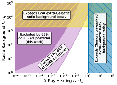
Figure 32: Models with excess high-redshift radio background can produce much larger power spectra than the standard scenario where the 21 cm brightness temperature is seen in contrast to the CMB. However, such models without accompanying X-ray heating of the IGM are excluded by HERA. Here we show the region of parameter space disfavored by 68% and 95% of HERA’s posterior, as well as regions inconsistent with either the LWA’s radio background measurements (Dowell & Taylor 2018) or Chandra’s X-ray background measurements (Lehmer et al. 2012). Between HERA’s constraints and Chandra’s, models where LWA’s extra-Galactic radio background as entirely explained by $z>8$ emission (i.e. models of the radio background at the bottom of the yellow region) are disfavored but not entirely excluded.

This space was already constrained by other measurements of astrophysical backgrounds. Reis et al. (2020) showed that models with strong $f_{\rm*}\cdot f_{r}$ are inconsistent with the radio background from LWA (Dowell & Taylor 2018) and ARCADE 2 (Fixsen et al. 2011; Seiffert et al. 2011), where the lower frequency measurements from LWA are the more constraining of the two (Reis et al. 2020). Likewise, Fialkov et al. (2017) show that large values of $f_{\rm*}\cdot f_{X}$ are generally ruled out by Chandra X-ray background measurements in the 0.5–2 keV band (Lehmer et al. 2012). We show those limits in Figure 32 in yellow and blue, respectively. Compared to the results in H22b, our new 21 cm constraints leave little room for the LWA radio background to be explained entirely as a cosmological signal originating from $z>8$. Such models are not entirely excluded, but they are mostly disfavored at 68% credibility or greater.

The second result, which is also an effect of the higher X-ray efficiency, can be seen via our derived constraints on the spin temperature of the IGM. In Figure 33, we show how HERA data updates our model’s prior on $\overline{T}_{S}$ and $\overline{T}_{\text{radio}}$.

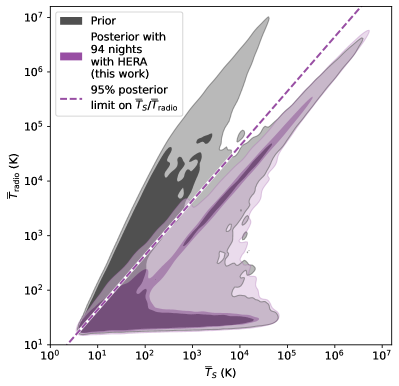
Figure 33: The derived constraints from our model with excess radio emission from high-redshift galaxies allows for a large range of both radio background and IGM spin temperatures at $z=7.9$. HERA generally favors models with lower radio background, though large radio backgrounds counteracted by large spin temperatures are still possible. Both temperatures are averaged over the neutral IGM where 21 cm emission or absorption might be observed. 95% of the posterior volume with HERA falls below the line where $\overline{T}_{S}/\overline{T}_{\text{radio}}=0.21$. Performing the same calculation with the $z=10.4$ posterior (not shown) we can constrain $\overline{T}_{S}/\overline{T}_{\text{radio}}>0.18$ at 95% credibility.

Both of these quantities are averaged over the neutral IGM at $z=7.9$.

In general, our results exclude models with large radio background temperatures without also featuring large spin temperatures. Specifically, our 95% credible interval requires that $\overline{T}_{S}/\overline{T}_{\text{radio}}>0.21$ at $z=7.9$. By performing the same calculation for Band 1, we can also show that at $z=10.4$, $\overline{T}_{S}/\overline{T}_{\text{radio}}>0.18$ with 95% credibility. While the posterior largely prefers relatively low radio background temperatures, there remain a set of models where a large radio background becomes coupled to the spin temperature, yielding $\overline{T}_{S}/\overline{T}_{\text{radio}}\approx 1$ and thus small power spectra.

7.6 Comparison of Astrophysical Models and Constraints

Finally, we can now more fully compare the results of our four models and their implications for the thermal history of the IGM. As we saw in Figure 27, the results from 21cmMC exhibit a more dramatic improvement at $z=7.9$ in this work relative to H22b than either of the phenomenological models (see Section 7.3) or the radio background model (see Section 7.5). In the discussion around Figure 31, we saw clear evidence that 21cmMC’s change in $\overline{T}_{S}$ and thus in the inferred posterior probability distribution of $\Delta^{2}$ was driven by the power spectrum constraints at $z=10.4$. This tight connection between redshifts requires rather rapid thermal evolution of the IGM, which is generally the case for the range of 21cmMC models we consider.

In the other models, the spin temperature history can evolve quite gradually, and thus yield similarly gradual 21 cm signal evolution that will be more difficult to disfavor with improved $z=10.4$ limits. For the reionization-driven model, this is because $\overline{T}_{S}$ is parameterized as a power-law in redshift with a uniform prior on the power-law index. In the radio background model, there are two reasons for gradual evolution. First, the stellar-mass-halo-mass relation is constant in the radio background model, which gives rise to a much more gradual cosmic star formation history than, e.g., models in which the relation is itself a function of halo mass. Second, because the radio and X-ray backgrounds are both sourced by galaxies, both $\overline{T}_{\rm radio}$ and $\overline{T}_{S}$ will grow similarly as the cosmic star formation rate density rises, resulting in relatively gradual evolution in the 21 cm signal. By contrast, in our 21cmMC simulations, $T_{\rm radio}=T_{\text{CMB}}$, which of course declines as $(1+z)$. This means $T_{\rm radio}/\overline{T}_{S}$ will evolve more rapidly than in than in the radio background models, even if both share an identical $\overline{T}_{S}$ history.

Another reason for the difference between models is the way 21cmMC directly incorporates data from other wavelengths (especially the galaxy luminosity function)—a major advantage of the approach. Models that fit the luminosity function at all redshifts require the star formation efficiency to increase with galaxy mass (at least up to galaxy masses comparable to the Milky Way, see e.g., Mirocha et al. 2017; Park et al. 2019). The 21cmMC models therefore also favor massive galaxies, whose abundance evolves quite rapidly at high redshifts. Because these galaxies are also the sources of IGM heating in this model, their rapidly evolving abundance also leads to rapid IGM heating. Because the luminosity function fits “bake in” this kind of behavior, 21cmMC models that feature modest heating at $z=10.4$ require stronger heating at $z=7.9$. The expected increase is roughly the ratio of the stellar mass density at the two redshifts, which is a factor of $\sim$3. This explains why the strong $\overline{T}_{S}$ limit in 21cmMC at $z=7.9$ is actually informed in large part by the ostensibly weaker temperature limits at $z=10.4$.

Of course, this conclusion is reliant on the parameterization of the galaxy luminosity function within 21cmMC. While a wide range of models agree that a physically-motivated extrapolation of the observed luminosity function to higher redshifts behaves similarly, it is of course reasonable to suppose that the extrapolation breaks down—perhaps because of processes unique to high-redshifts, or perhaps simply because young dwarf galaxies behave differently than their larger cousins (see e.g., Qin et al. 2020). One could always broaden the allowed set of galaxy models to accommodate such exotic astrophysics. We have, of course, explored one class of such models by examining the effect of an excess radio background in Section 7.5. One could also imagine adding another source of early heating like Pop III remnants that could inject sufficient heat into the IGM at $z=10.4$ without necessarily affecting the constraints at $z=7.9$, though this might require some degree of fine tuning—a question left for future work. Regardless, it is useful to understand how we should interpret the HERA limits in the context of “vanilla” galaxy models. Here, the 21cmMC results demonstrate that the “known” galaxy population requires substantial IGM heating by $z\sim 8$.

Regardless of the differences between our models, we should not lose sight of the fact that they are all pointing in fundamentally the same direction: a heated IGM during the EoR. To put them in the broader cosmological context of other 21 cm experiments, we compare them to a few illustrative scenarios for the thermal history of the IGM in Figure 34.

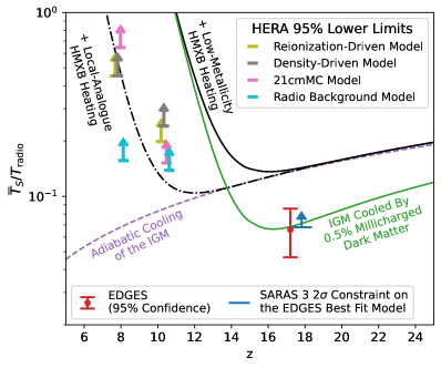
Figure 34: To put the results from our four models in Figure 27 into their cosmological context, we show each model’s 95% credible limits on $\overline{T}_{S}/T_{\text{radio}}$. Each model’s results are shown offset from their proper redshifts, 7.9 or 10.4, for visual clarity. They differ in their conclusions, both due to their different physical assumptions as well as their different priors and incorporation of other high-redshift probes. However, they all conclude that the IGM spin temperature at both $z=7.9$ and $z=10.4$ is in excess of the temperature one would expect from adiabatic cooling since recombination, assuming $T_{\text{radio}}=T_{\text{CMB}}$ (purple dashed line). They are also generally inconsistent with an IGM weakly heated by X-rays (black dot-dashed line), as it would be if the local relation for $L_{X}/{\rm SFR}$ for HMXBs held at high redshift (see Figure 28)—although that statement is somewhat model dependent. However, all our models are consistent with a more rapidly heated IGM, such as the one shown as a solid black line where $L_{\rm X<2keV}/{\rm SFR}=10^{41}$ erg s^-1 ${\rm M}_{\odot}^{-1}$ yr, which is closer to the expectation for low-metallicity HMXBs. To put HERA’s result in the context of high-redshift global signal measurements, we also show results from EDGES (Bowman et al. 2018) and SARAS 3 (Singh et al. 2022). For EDGES, we show the implied $\overline{T}_{S}/T_{\text{radio}}$ from the depth of their best fit model, as well as the $2\sigma$ range of model amplitudes. For SARAS, which disfavors the EDGES best fit at $\sim$95% confidence when marginalizing over only the amplitude, we show the lower limit on models with the same shape as the EDGES signal. The SARAS central redshift is also offset from EDGES for visual clarity. Finally, we show a model with 0.5% millicharged dark matter, as in Figure 11 of H22b, which could explain EDGES and still be consistent with HERA if there is sufficient X-ray heating between $z\sim 17$ and $z\sim 10$.

The arrows show the lower bounds of the 95% credible regions of $\overline{T}_{S}/T_{\text{radio}}$ at $z=7.9$ and $z=10.4$ inferred by each of the four models. We also show the expectation for an IGM temperature set by adiabatic cooling since recombination with no additional heating from astrophysical sources. Just as Figure 27 showed, the lower limits at both redshifts are above this curve, requiring substantial X-ray heating (as illustrated by the solid black line where $L_{\rm X<2keV}/{\rm SFR}=10^{41}$ erg s^-1 ${\rm M}_{\odot}^{-1}$ yr). This is a significant improvement from H22b, which could not demonstrate any heating beyond the adiabatic cooling curve at $z=10.4$. More interestingly, they are all inconsistent with an IGM thermal history that one would predict by extrapolating the local relation between X-ray luminosity and star formation rate to high redshift (black dot-dashed line, see Figure 28). The accordance of multiple models here strengthens the argument in Section 7.4.1 that our results broadly favor an IGM heated by low-metallicity HMXBs.

Figure 34 also shows measurements at higher redshifts. The EDGES result (Bowman et al. 2018) found a surprisingly large absorption signal at $z\sim 17$, requiring either substantial cooling of the gas below the adiabatic limit or a larger radio background than provided by the CMB. The implied range of $\overline{T}_{\rm S}/T_{\rm radio}$ is shown by the red error bars, but note that EDGES found this absorption trough to be very narrow, implying that the Universe was heated shortly afterward. However, the recent SARAS 3 measurement (Singh et al. 2022) did not detect such a signal; the upper limit is subtle to express quantitatively, but here we show the limit their measurement places on a feature with the shape of the best-fit EDGES signal with an unknown amplitude. Though we show the SARAS 3 limit offset in redshift for clarity, the measurement spanned a wide frequency range corresponding to $15.8<z<24.6$.

Because HERA observed at much smaller redshifts than EDGES and SARAS 3, it is difficult to compare directly—even if the deep EDGES trough is real, any heating between $z\sim 15$ and $z\sim 10$ (as indeed the EDGES best-fit model requires!) would make the two measurements consistent. We show an example of such a model (green solid line) where the IGM is cooled by interactions with a fraction (0.5%) of millicharged dark matter with mass 10 MeV and charge $10^{-5}$ times that of the electron, following Muñoz & Loeb (2018). The gas is subsequently heated by HMXBs. This model is designed to explain EDGES and still be consistent with lower redshift observations like HERA’s, though it is in mild tension with SARAS 3. More independent measurements like SARAS 3, as well as low-frequency power spectra from HERA Phase II and other interferometers, will be extremely valuable in understanding this early era and any new physics that may have impacted it.

8 Conclusion

In this work we have presented improved upper limits on the 21 cm power spectrum using 94 nights of observing with Phase I of the Hydrogen Epoch of Reionization Array (HERA), as well as their astrophysical implications for the X-ray heating of the IGM. We have found with 95% confidence that $\Delta^{2}(k=\text{0.34\,$h$Mpc${}^{-1}${}})\leq\text{457\,mK${}^{2}${}}$ at $z=7.9$ and that $\Delta^{2}(k=\text{0.36\,$h$Mpc${}^{-1}${}})\leq\text{3,496\,mK${}^{2}${}}$ at $z=10.4$, an improvement by a factor of 2.1 and 2.6 respectively over previous HERA limits in H22a with 18 nights of data and roughly the same number of antennas. Our full set of upper limits across $k$ are detailed in Section 5.

Our results rely heavily on the application of existing techniques to this new data set. In particular, we adapted most of the techniques used in H22a to our larger data volume, noting where and why we made different analysis choices. We replicated many of the statistical tests developed in H22a—and some new ones—to show that our data largely integrate down as expected and that our techniques for systematics mitigation do not introduce any new biases. Likewise, we have performed a number of the simulation-based tests developed in Aguirre et al. (2022) using our updated techniques, including an end-to-end test of our analysis pipeline that simulates the full data volume before reducing it to power spectra. While many small adjustments were made to accommodate the larger data set considered here, the fundamental philosophical approach remains the same. Instead of subtracting or filtering foregrounds, we focused on maintaining spectral smoothness and systematics control while minimizing and rigorously quantifying potential sources of signal loss.

We also revisit four independent theoretical models for inferring constraints on IGM and galaxy properties during the EoR and the cosmic dawn. These techniques were applied to the H22a data set in H22b where we showed that the IGM had to heated above the adiabatic cooling limit by at least $z=7.9$. Using the improved upper limits presented in this work, the four techniques broadly agree with at least 95% of their posterior volumes (and in some cases greater than 99%): the IGM had to be heated above the expectation from adiabatic cooling by at $z=10.4$ the latest.

There are two key consequences of this result. The first follows from our current understanding from existing probes of reionization—especially the integrated optical depth to reionization, galaxy UV luminosity functions, and quasar spectroscopy—that the bulk of reionization happens after $z=10.4$. If that is the case, then we have ruled out the “cold reionization” scenarios in which the IGM continues to adiabatically cool until it reionizes, creating a bright 21 cm power spectrum is boosted by a strong contrast between the CMB and the IGM spin temperature. It is still possible that the IGM is slightly heated at $z=10.4$ but still colder than the CMB. However, a broad class of models where the IGM remains very cold until reionization are no longer viable.

Second, if high mass X-ray binaries dominate the soft X-ray budget of high redshift galaxies and thus were responsible for the heating of the IGM, as is generally expected (Fragos et al. 2013), then more than 99% of HERA’s posterior excludes the local relationship between star formation and soft X-ray production (Mineo et al. 2012) extrapolated to high redshift. We instead favor models with low-metallicity HMXBs, which is clear evidence for the impact on the IGM of some of the first compact objects to form during the cosmic dawn.

We also used a semi-numerical model that allows galaxies to create radio backgrounds brighter than the CMB to jointly constrain those radio backgrounds and the X-ray luminosity of those galaxies. Specifically, we combined HERA limits (which disfavor strong radio backgrounds with weak X-ray heating) and Chandra X-ray background constraints (which rule out strong X-ray heating) to exclude most models that would explain the radio backgrounds observed by LWA and ARCARDE 2 as originating at $z\gtrsim 8$.

Looking forward, we see a number of ways HERA might continue to improve the constraints on the 21 cm signal as we continue the steady march to greater and greater sensitivity. One approach would be to move beyond cautious foreground-avoidance and attempt to apply more aggressive and more nearly optimal filters, removing foregrounds (Ewall-Wice et al. 2021) in delay space and integrating down coherently for longer with better-tailored fringe-rate filters (Parsons et al. 2016). These techniques might help us explore more frequency bands and claw back some of the most sensitive baselines that we had to excise in this work. However, they will likely incur higher levels of signal loss that will have to be rigorously quantified and taken into account.

More importantly, this analysis only used a small fraction of HERA’s final size and bandwidth. HERA Phase II, now being commissioned, will have 350 antennas observing from 50–250 MHz which corresponds to $4.7<z<27.4$. We now have a well-tested analysis pipeline taking us all the way to power spectra and astrophysical inference, including a suite of statistical tests and end-to-end simulations with which to validate our results. This work, along with H22a, H22b, and their supporting papers, will serve as a foundation for future HERA analysis. Of course, HERA Phase II has an entirely new signal chain—from feeds to correlator—and will likely have to contend with a somewhat different set of systematics. However, if these can be overcome, HERA could be the instrument to detect and characterize the 21 cm power spectrum from the epoch of reionization and push our knowledge of early stars, black holes, and galaxies into the cosmic dawn.

Appendix A A Physical Model for HERA Phase I Crosstalk Systematics

One of the most important systematics that we needed to mitigate before estimating power spectra is been crosstalk. The strategy developed in Kern et al. (2019), demonstrated in Kern et al. (2020b), and applied in H22a is quite effective at removing that crosstalk. However, as we discovered in Section 3.2.4, our crosstalk was significantly less time-stable over the entire season that it was during the 18 nights analyzed in H22a. This motivated LST-binning over epochs and new cuts on the data (see Section 3.3.2).

This discovery also motivated a renewed attempt to understand the physical origin of the crosstalk. We began with the basic mathematical model of crosstalk presented in Kern et al. (2019). If we postulate that the voltage measured on an antenna $i$ is due to both the incident sky signal $v_{i}$ absorbed by antenna $i$ and contributions from other antennas, we can write that voltage (ignoring noise) as

$$v_{i}^{\prime}=v_{i}+\sum_{n\neq i}\varepsilon_{ni}v_{n},$$ (A1)

where $\varepsilon_{ni}$ is the coupling between the $n$th antenna and antenna $i$. Since visibilities are formed by cross-correlating voltages, a visibility with cross-coupling takes the form

$$V^{\prime}_{ij}=\langle(v_{i}+\sum_{n\neq i}\varepsilon_{ni}v_{n})(v_{j}+\sum_{n\neq j}\varepsilon_{nj}v_{n})^{*}\rangle$$ (A2)

where angle brackets indicate a time average. Assuming the coupling is small and dropping all terms that are second order in $\varepsilon$ or first order in $\varepsilon$ but only involve cross-correlations, we get

$$V^{\prime}_{ij} \approx\langle v_{i}v_{j}*+\varepsilon_{ij}^{*}v_{i}v_{i}^{*}+\varepsilon_{ji}v_{j}v_{j}^{*}\rangle$$

$$\approx V_{ij}+\varepsilon_{ij}^{*}V_{ii}+\varepsilon_{ji}V_{jj}.$$ (A3)

Thus, to leading order, the main cross-coupling contributions appear as autocorrelations of each antenna involved leaking into a visibility. It should be noted that we are ignoring antenna-to-antenna coupling effects due to reflections off antennas, which Josaitis et al. (2022) showed would be an important systematic for HERA Phase II. At this point, we have seen no evidence that this is a dominant systematic for HERA Phase I.

Kern et al. (2019) was agnostic as to the origin of the coupling. They instead focused on how autocorrealtions, which evolve much more slowly in time than cross-correlations with any appreciable east-west projected length, can be distinguished from the primary sky signal in fringe-rate space. As long as $\varepsilon$ was time-stable, its structure was of secondary concern. Our observation of discontinuities in the crosstalk in delay space (see Figure 6) meant that $\varepsilon$ was effectively no longer stable over a full season of LST-binned data.

Explaining the range of delays over which crosstalk was observed in e.g. Figure 6 and Figure 7—generally 800 to $\sim$2000 ns—required solving a puzzle. Those delays are too long to be explained by a broadcasting antenna, which would created correlated signals at delays explicable by the light travel time across the array. They are also too short to be explained by invoking cable reflections, which require two traversals of the $\sim$150 m cables connecting antennas to the receivers and thus take $\sim$1200 ns. Kern & Parsons (2019) explored and rejected several possible explanations. No model could explain that range of delays and also the asymmetric structure we see in a single visibility, whose positive and negative delays can exhibit completely different crosstalk structure.

However, Kern & Parsons (2019) did note that attributing positive or negative delays to the first and second antennas in a baseline reveals interesting patterns in the dependence of the delay and amplitude of the cross-talk peak on position in the array. That proved to be a key insight. Taking the time-averaged amplitude of the Fourier transform of a several inpainted visibilities from a single epoch (in this case Epoch 2) which share one antenna in common illustrates that pattern. In Figure 35 we show this for a subset of the baselines that share antenna 119, all of them in the same two rows (see Figure 4).

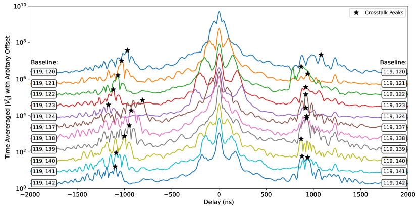
Figure 35: Examining the time-averaged delay spectrum of several baselines all sharing a single antenna reveals a clear pattern in the delay structure of the crosstalk feature between $800\lesssim|\tau|\lesssim 1500$ ns, but only one on side. Here we show eleven baselines all sharing antenna 119 (and all north-polarized). All the antennas are part of two rows (see Figure 4). We plot their time-averaged amplitudes in delay space, each arbitrarily offset for readability. We also mark the peak delays of each baseline’s crosstalk with black stars, which our model must explain. Crosstalk at negative delay shows similar structure within rows of the array (120–124 as compared to 137–142) with diminishing amplitude as we move eastward. By contrast, the crosstalk feature at positive delay shows no clear pattern. This supports the argument that the negative delay feature is associated with antenna 119. It follows from symmetry that, since this effect is not unique to antenna 119, the positive delay feature must be associated with the other antenna. At low delay we can also see the foregrounds peak in the main lobe of the primary beam, as well as a widening “pitchfork” feature associated with foregrounds on the horizon (Thyagarajan et al. 2015a, b; Pober et al. 2016), which is at higher delay for longer baselines.

What we see is a remarkable asymmetry between positive and negative delays. At negative delay, we see a delay structure that looks similar within rows, but with decreasing amplitude and at more negative delays as the second antenna moves east. Meanwhile, at the crosstalk systematics at positive delay show up at largely similar delays but with wildly ranging amplitudes and structures. Holding a single antenna fixed and seeing such similarities at negative delays indicates a clear association between antenna $i$ and negative delays in $V_{ij}$—and thus by symmetry, an association between antenna $j$ and positive delays. A model for this crosstalk must explain how the voltage signal from e.g. antenna 119 was received by every other antenna with a position-dependent peak delay and amplitude.

To understand these delays, recall that HERA Phase I reused PAPER feeds and signal chains. These included $\sim$150 m coaxial cables from each feed to a set of eight “receiverators,” RF-shielded mini-fridges each containing 16 receiver and post-amplification modules (Bradley 2017), located just west of the array. These were then connected by $\sim$20 m coaxial cables to a shipping container housing the analog to digital converters and the correlator (DeBoer 2015). We hypothesize that at one of those connection points, likely after the receiverators, was leaking and broadcast virtually every antenna’s voltage signal. These signals were then picked up by every other antenna, leading to autocorrelations appearing in cross-correlation visibilities at high delay. We thus explain the crosstalk peak delays and amplitudes in Figure 35 with a model for $\varepsilon_{ij}$ where

$$\varepsilon_{ij}\approx A_{i}\left(\frac{d_{*j}}{\rm 1\,m}\right)^{-\alpha}\exp\left[2\pi i\nu\left(\tau_{i,{\rm cable}}+d_{*j}/c+\tau_{\rm offset}\right)\right].$$ (A4)

Here $\tau_{i,{\rm cable}}$ is the light travel time along the $\sim$150 m cable connecting antenna $i$ to the receiverators; it can be easily measured by examining the delay spectrum of autocorrelations since cable reflections appear at $2\tau_{i,{\rm cable}}$ (Kern et al. 2020b). The rest of the terms are free parameters. The first two are the positions of the emitter, $x_{*}$ and $y_{*}$, from which we can calculate $d_{*j}$, the distance from the emitter to antenna $j$. The next is $\tau_{\rm offset}$ which can account for the possibility that emission occurred after traversing another $\sim$20 m cable between the receiverators and the correlation. No per-antenna variation is allowed in $\tau_{\rm offset}$. Finally, the amplitude of the crosstalk seen on each baseline depends on the “leakiness” of antenna $i$—$A_{i}$, each a free parameter—and the distance it must travel to the power $-\alpha$. Since emitted voltages go down as $1/r$, we should expect $\alpha=1$. However, to attempt to account for the effects of complicated mutli-path propagation through a lattice of antennas, we leave $\alpha$ as a free parameter.

Since this model does not predict the full delay spectrum of the crosstalk, our goal here is not to solve for every parameter optimally. Instead, we want to test its physical plausibility. Therefore, we fit both parts—the phase and the amplitude—separately with potentially different emitter positions. First we fit the delays, since that is a simpler model with far fewer free parameters. In Figure 36, we show in the left panel the measured crosstalk peak positions at negative delay (black stars in Figure 35) for all baselines $V_{ij}$ where $i=119$.

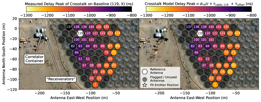
Figure 36: We can predict the measured peak delays in the crosstalk in each visibility $V_{ij}$ using a model (Equation A4) where antenna $i$’s signal travels down a $\sim$150 m cable, gets amplified in the “receiverators,” and then is emitted shortly thereafter. That voltage signal then travels over the air and is picked up by antenna $j$, producing a contribution of $V_{ii}$ to $V_{ij}$ at large negative delays (Equation A3). In the left-hand panel, we show all such measurements involving a single antenna, 119, and the prediction of our best fit model (right-hand panel) using all baselines. We overlay our data and fit over recent satellite imagery of HERA from Google Maps (accessed in June 2022), which shows that our best fit for the position of the emitter is spatially consistent with our receiverators and correlator container. This explanation of the physical origin of the crosstalk validates our approach to removing it.

In the right panel, we show our best fit source position and the prediction for the total delay term in Equation A4. Both are overlaid over recent satellite photography of HERA. This fit is performed over all unflagged baselines, with the exception of a few baseline that had too little crosstalk to measure the peak reliably. The fit is quite good; the average delay error is only 47 ns which is only a few times larger than the 12.8 ns delay resolution of the Fourier transform after removing flagged channels. More tellingly, the emitter position is quite consistent with the suspect signal chain elements, namely the connections between the receiverators and the correlator. The fit $\tau_{\rm offset}=99$ ns which consistent with expectations for the for the $\sim$20 m cable (Kern et al. 2020b), given the speed of light in the medium. While this result lends significant credence for our model, we cannot definitively state that it locates the emitter as the input ports on the correlator container. The emitter position and $\tau_{\rm offset}$ are correlated and, as Figure 35 shows, quantifying the error in measuring peak delays is challenging.

As a second test, we also fit the amplitude of each crosstalk signal using Equation A4. This test is a bit less straightforward, since it requires a free parameter $A_{i}$ for every antenna. That said, an independent fit of the emitter position yields a quite consistent result, as we can see in Figure 37.

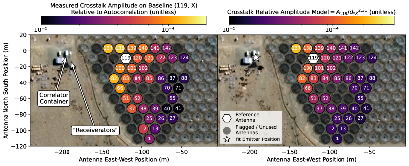
Figure 37: Analogously to Figure 36, we can also predict the amplitudes of the crosstalk as they appear in each baseline using the same model (Equation A4). In the left-hand panel we show measured peak crosstalk amplitudes, relative to the autocorrelations that source them, for all baselines involving antenna 119. On the right, we show the best-fit model prediction for that same data set using all baselines. The relatively good agreement here, as well as the fact that we find a consistent emitter position despite fitting for it independently fit, lend credence to our physical model for the crosstalk.

Again, we show the crosstalk amplitudes associated with antenna 119 (left-hand panel) but perform our fit over all baselines. The result is a fairly good fit, with a mean amplitude error of $1.2\times 10^{-5}$ relative to the autocorrelations. Oddly, the best fit power law is not $\alpha=1$ as we had expected, but $\alpha=2.31$. We do not have an explanation for why it should follow that power law, though we note that the problem is a fair bit more complicated than simple free-space propagation. There are also some parameter degeneracies to consider; one can still get a decent fit by fixing $\alpha=1$ and moving the emitter position much closer to the array.

Without a proper error analysis, it is difficult to validate the precise parameterization of our model. What should $\alpha$ be? What about $\tau_{\rm offset}$? Can we explain the full delay structure of the crosstalk signal as some sort of multi-path propagation effect? Can construction of new antennas explain the epoch-to-epoch change in the crosstalk we saw in Figure 6? Unfortunately we can only speculate. The system in question has long-since been disassembled and HERA Phase II does not use receiverators nor does this systematic appear in more recent data. That said, having a plausible physical mechanism that allows autocorrelations to leak into cross-correlations in a relatively time-stable way adds significant support to our strategy for removing the systematic.

References

- Abdurashidova et al. (2022a) Abdurashidova, Z., Aguirre, J. E., Alexander, P., et al. 2022a, The Astrophysical Journal, 925, 221, doi: 10.3847/1538-4357/ac1c78
- Abdurashidova et al. (2022b) —. 2022b, The Astrophysical Journal, 924, 51, doi: 10.3847/1538-4357/ac2ffc
- Aguirre et al. (2022) Aguirre, J. E., Murray, S. G., Pascua, R., et al. 2022, The Astrophysical Journal, 924, 85, doi: 10.3847/1538-4357/ac32cd
- Asad et al. (2018) Asad, K. M. B., Koopmans, L. V. E., Jelić, V., et al. 2018, MNRAS, 476, 3051, doi: 10.1093/mnras/sty258
- Asad et al. (2016) —. 2016, MNRAS, 462, 4482, doi: 10.1093/mnras/stw1863
- Astropy Collaboration et al. (2018) Astropy Collaboration, Price-Whelan, A. M., SipHocz, B. M., et al. 2018, AJ, 156, 123, doi: 10.3847/1538-3881/aabc4f
- Barkana (2018) Barkana, R. 2018, Nature, 555, 71, doi: 10.1038/nature25791
- Barry et al. (2016) Barry, N., Hazelton, B., Sullivan, I., Morales, M., & Pober, J. 2016, MNRAS, 461, 3135, doi: 10.1093/mnras/stw1380
- Barry et al. (2019) Barry, N., Wilensky, M., Trott, C. M., et al. 2019, ApJ, 884, 1, doi: 10.3847/1538-4357/ab40a8
- Beardsley et al. (2016) Beardsley, A., Hazelton, B., Sullivan, I., et al. 2016, ApJ, 833, 102, doi: 10.3847/1538-4357/833/1/102
- Bernardi et al. (2016) Bernardi, G., Zwart, J. T. L., Price, D., et al. 2016, MNRAS, 461, 2847, doi: 10.1093/mnras/stw1499
- Bevins et al. (2021) Bevins, H. T. J., Handley, W. J., Fialkov, A., de Lera Acedo, E., & Javid, K. 2021, MNRAS, 508, 2923, doi: 10.1093/mnras/stab2737
- Bosman & Becker (2015) Bosman, S. E. I., & Becker, G. D. 2015, MNRAS, 452, 1105, doi: 10.1093/mnras/stv1336
- Bouwens et al. (2015) Bouwens, R., Illingworth, G., Oesch, P., et al. 2015, ApJ, 803, 34, doi: 10.1088/0004-637X/803/1/34
- Bouwens et al. (2016) Bouwens, R. J., Oesch, P. A., Illingworth, G. D., Ellis, R. S., & Stefanon, M. 2016, ArXiv e-prints:1610.00283. https://arxiv.org/abs/1610.00283
- Bowman et al. (2018) Bowman, J. D., Rogers, A. E. E., Monsalve, R. A., Mozdzen, T. J., & Mahesh, N. 2018, Nature, 555, 67, doi: 10.1038/nature25792
- Bradley (2017) Bradley, R. F. 2017, URSI Radio Science Bulletin, 2017, 39, doi: 10.23919/URSIRSB.2017.8267372
- Bradley et al. (2019) Bradley, R. F., Tauscher, K., Rapetti, D., & Burns, J. O. 2019, ApJ, 874, 153, doi: 10.3847/1538-4357/ab0d8b
- Brandenberger et al. (2019) Brandenberger, R., Cyr, B., & Shi, R. 2019, J. Cosmology Astropart. Phys, 2019, 009, doi: 10.1088/1475-7516/2019/09/009
- Bull (2021) Bull, P. 2021, HERA Memo #98: Mathematical description of the vis_cpu visibility simulator, Tech. rep.
- Byrne et al. (2021) Byrne, R., Morales, M. F., Hazelton, B. J., & Wilensky, M. 2021, Monthly Notices of the Royal Astronomical Society, 503, 2457, doi: 10.1093/mnras/stab647
- Byrne et al. (2019) Byrne, R., Morales, M. F., Hazelton, B., et al. 2019, ApJ, 875, 70, doi: 10.3847/1538-4357/ab107d
- Carilli et al. (2020) Carilli, C. L., Thyagarajan, N., Kent, J., et al. 2020, The Astrophysical Journal Supplement Series, 247, 67, doi: 10.3847/1538-4365/ab77b1
- Carroll et al. (2016) Carroll, P. A., Line, J., Morales, M. F., et al. 2016, Monthly Notices of the Royal Astronomical Society, 461, 4151, doi: 10.1093/mnras/stw1599
- Cheng et al. (2018) Cheng, C., Parsons, A. R., Kolopanis, M., et al. 2018, ApJ, 868, 26, doi: 10.3847/1538-4357/aae833
- Choudhuri et al. (2021) Choudhuri, S., Bull, P., & Garsden, H. 2021, MNRAS, 506, 2066, doi: 10.1093/mnras/stab1795
- Ciardi & Ferrara (2005) Ciardi, B., & Ferrara, A. 2005, Space Sci. Rev., 116, 625, doi: 10.1007/s11214-005-3592-0
- Cohen et al. (2020) Cohen, A., Fialkov, A., Barkana, R., & Monsalve, R. A. 2020, MNRAS, 495, 4845, doi: 10.1093/mnras/staa1530
- Datta et al. (2010) Datta, A., Bowman, J., & Carilli, C. 2010, ApJ, 724, 526, doi: 10.1088/0004-637X/724/1/526
- de Oliveira-Costa et al. (2008) de Oliveira-Costa, A., Tegmark, M., Gaensler, B. M., et al. 2008, MNRAS, 388, 247, doi: 10.1111/j.1365-2966.2008.13376.x
- DeBoer (2015) DeBoer, D. 2015, HERA Phase I Feed Design, Tech. rep., Department of Astronomy, University of California, Berkeley, CA
- DeBoer et al. (2017) DeBoer, D., Parsons, A., Aguirre, J., et al. 2017, PASP, 129, 45001, doi: 10.1088/1538-3873/129/974/045001
- Dillon & Parsons (2016) Dillon, J., & Parsons, A. 2016, ApJ, 826, 181, doi: 10.3847/0004-637X/826/2/181
- Dillon et al. (2014) Dillon, J., Liu, A., Williams, C., et al. 2014, Phys. Rev. D, 89, 23002, doi: 10.1103/PhysRevD.89.023002
- Dillon et al. (2015a) Dillon, J., Neben, A., Hewitt, J., et al. 2015a, Phys. Rev. D, 91, 123011, doi: 10.1103/PhysRevD.91.123011
- Dillon et al. (2015b) Dillon, J., Tegmark, M., Liu, A., et al. 2015b, Phys. Rev. D, 91, 23002, doi: 10.1103/PhysRevD.91.023002
- Dillon (2021a) Dillon, J. S. 2021a, HERA Memo #97: H1C Internal Data Release 3.2, Tech. rep.
- Dillon (2021b) —. 2021b, HERA Memo #107: H1C IDR 3.2 Power Spectrum Analysis Updates and Choices, Tech. rep.
- Dillon et al. (2021) Dillon, J. S., Kern, N., & Parsons, A. R. 2021, HERA Memo #104: A Physical Model for the H1C Cross-Talk Systematic, Tech. rep.
- Dillon et al. (2013) Dillon, J. S., Liu, A., & Tegmark, M. 2013, Physical Review D, 87, doi: 10.1103/physrevd.87.043005
- Dillon et al. (2018) Dillon, J. S., Kohn, S. A., Parsons, A. R., et al. 2018, MNRAS, 477, 5670, doi: 10.1093/mnras/sty1060
- Dillon et al. (2020) Dillon, J. S., Lee, M., Ali, Z. S., et al. 2020, arXiv e-prints, arXiv:2003.08399. https://arxiv.org/abs/2003.08399
- Dowell & Taylor (2018) Dowell, J., & Taylor, G. B. 2018, ApJ, 858, L9, doi: 10.3847/2041-8213/aabf86
- Eastwood et al. (2019) Eastwood, M. W., Anderson, M. M., Monroe, R. M., et al. 2019, AJ, 158, 84, doi: 10.3847/1538-3881/ab2629
- Ewall-Wice et al. (2018) Ewall-Wice, A., Chang, T.-C., Lazio, J., et al. 2018, The Astrophysical Journal, 868, 63, doi: 10.3847/1538-4357/aae51d
- Ewall-Wice et al. (2020) Ewall-Wice, A., Chang, T.-C., & Lazio, T. J. W. 2020, MNRAS, 492, 6086, doi: 10.1093/mnras/stz3501
- Ewall-Wice et al. (2017) Ewall-Wice, A., Dillon, J. S., Liu, A., & Hewitt, J. 2017, MNRAS, 470, 1849, doi: 10.1093/mnras/stx1221
- Ewall-Wice et al. (2014) Ewall-Wice, A., Dillon, J. S., Mesinger, A., & Hewitt, J. 2014, Monthly Notices of the Royal Astronomical Society, 441, 2476, doi: 10.1093/mnras/stu666
- Ewall-Wice et al. (2016a) Ewall-Wice, A., Hewitt, J., Mesinger, A., et al. 2016a, MNRAS, 458, 2710, doi: 10.1093/mnras/stw452
- Ewall-Wice et al. (2016b) Ewall-Wice, A., Dillon, J., Hewitt, J., et al. 2016b, MNRAS, 460, 4320, doi: 10.1093/mnras/stw1022
- Ewall-Wice et al. (2016) Ewall-Wice, A., Bradley, R., Deboer, D., et al. 2016, ApJ, 831, 196, doi: 10.3847/0004-637X/831/2/196
- Ewall-Wice et al. (2021) Ewall-Wice, A., Kern, N., Dillon, J. S., et al. 2021, MNRAS, 500, 5195, doi: 10.1093/mnras/staa3293
- Fagnoni et al. (2020) Fagnoni, N., de Lera Acedo, E., Drought, N., et al. 2020, arXiv e-prints, arXiv:2009.07939. https://arxiv.org/abs/2009.07939
- Fagnoni et al. (2021) Fagnoni, N., de Lera Acedo, E., DeBoer, D. R., et al. 2021, MNRAS, 500, 1232, doi: 10.1093/mnras/staa3268
- Feng & Holder (2018) Feng, C., & Holder, G. 2018, The Astrophysical Journal, 858, L17, doi: 10.3847/2041-8213/aac0fe
- Feroz et al. (2009) Feroz, F., Hobson, M. P., & Bridges, M. 2009, MNRAS, 398, 1601, doi: 10.1111/j.1365-2966.2009.14548.x
- Fialkov & Barkana (2019) Fialkov, A., & Barkana, R. 2019, MNRAS, 486, 1763, doi: 10.1093/mnras/stz873
- Fialkov et al. (2014) Fialkov, A., Barkana, R., & Visbal, E. 2014, Nature, 506, 197, doi: 10.1038/nature12999
- Fialkov et al. (2017) Fialkov, A., Cohen, A., Barkana, R., & Silk, J. 2017, MNRAS, 464, 3498, doi: 10.1093/mnras/stw2540
- Fixsen et al. (2011) Fixsen, D. J., Kogut, A., Levin, S., et al. 2011, ApJ, 734, 5, doi: 10.1088/0004-637X/734/1/5
- Foreman-Mackey et al. (2013) Foreman-Mackey, D., Hogg, D., Lang, D., & Goodman, J. 2013, PASP, 125, 306, doi: 10.1086/670067
- Fragos et al. (2013) Fragos, T., Lehmer, B., Tremmel, M., et al. 2013, ApJ, 764, 41, doi: 10.1088/0004-637X/764/1/41
- Franzen et al. (2019) Franzen, T. M. O., Vernstrom, T., Jackson, C. A., et al. 2019, Publications of the Astronomical Society of Australia, 36, e004, doi: 10.1017/pasa.2018.52
- Fraser et al. (2018) Fraser, S., Hektor, A., Hütsi, G., et al. 2018, Physics Letters B, 785, 159, doi: 10.1016/j.physletb.2018.08.035
- Furlanetto et al. (2006) Furlanetto, S., Oh, S., & Briggs, F. 2006, Phys. Rep., 433, 181, doi: 10.1016/j.physrep.2006.08.002
- Furlanetto et al. (2004) Furlanetto, S., Zaldarriaga, M., & Hernquist, L. 2004, ApJ, 613, 1, doi: 10.1086/423025
- Garsden et al. (2021) Garsden, H., Greenhill, L., Bernardi, G., et al. 2021, Monthly Notices of the Royal Astronomical Society, 506, 5802, doi: 10.1093/mnras/stab1671
- Gehlot et al. (2019) Gehlot, B. K., Mertens, F. G., Koopmans, L. V. E., et al. 2019, MNRAS, 488, 4271, doi: 10.1093/mnras/stz1937
- Georgiev et al. (2022) Georgiev, I., Mellema, G., Giri, S. K., & Mondal, R. 2022, MNRAS, 513, 5109, doi: 10.1093/mnras/stac1230
- Ghara et al. (2020) Ghara, R., et al. 2020, Monthly Notices of the Royal Astronomical Society, 493, 4728, doi: 10.1093/mnras/staa487
- Gorce et al. (2022) Gorce, A., Ganjam, S., Liu, A., et al. 2022, doi: 10.48550/ARXIV.2210.03721
- Górski et al. (2005) Górski, K. M., Hivon, E., Banday, A. J., et al. 2005, ApJ, 622, 759, doi: 10.1086/427976
- Greig & Mesinger (2015) Greig, B., & Mesinger, A. 2015, MNRAS, 449, 4246, doi: 10.1093/mnras/stv571
- Greig & Mesinger (2017) —. 2017, Proceedings of the International Astronomical Union, 12, 18, doi: 10.1017/s1743921317011103
- Greig et al. (2022) Greig, B., Mesinger, A., Davies, F. B., et al. 2022, Monthly Notices of the Royal Astronomical Society, 512, 5390, doi: 10.1093/mnras/stac825
- Greig et al. (2016) Greig, B., Mesinger, A., & Pober, J. 2016, MNRAS, 455, 4295, doi: 10.1093/mnras/stv2618
- Handley et al. (2015a) Handley, W. J., Hobson, M. P., & Lasenby, A. N. 2015a, Monthly Notices of the Royal Astronomical Society: Letters, 450, L61, doi: 10.1093/mnrasl/slv047
- Handley et al. (2015b) —. 2015b, Monthly Notices of the Royal Astronomical Society, 453, 4384, doi: 10.1093/mnras/stv1911
- Harris et al. (2020) Harris, C. R., Millman, K. J., van der Walt, S. J., et al. 2020, Nature, 585, 357–362, doi: 10.1038/s41586-020-2649-2
- Hazelton et al. (2017) Hazelton, B. J., Jacobs, D. C., Pober, J. C., & Beardsley, A. P. 2017, The Journal of Open Source Software, 2, 140, doi: 10.21105/joss.00140
- Hills et al. (2018) Hills, R., Kulkarni, G., Meerburg, P. D., & Puchwein, E. 2018, Nature, 564, E32, doi: 10.1038/s41586-018-0796-5
- Hogan & Rees (1979) Hogan, C., & Rees, M. 1979, MNRAS, 188, 791, doi: 10.1093/mnras/188.4.791
- Högbom (1974) Högbom, J. A. 1974, A&AS, 15, 417
- Hogg (1999) Hogg, D. W. 1999, arXiv e-prints, astro. https://arxiv.org/abs/astro-ph/9905116
- Hunter (2007) Hunter, J. D. 2007, Computing in Science & Engineering, 9, 90, doi: 10.1109/MCSE.2007.55
- Hurley-Walker et al. (2017) Hurley-Walker, N., Callingham, J. R., Hancock, P. J., et al. 2017, MNRAS, 464, 1146, doi: 10.1093/mnras/stw2337
- Jacobs et al. (2016) Jacobs, D. C., Hazelton, B. J., Trott, C. M., et al. 2016, The Astrophysical Journal, 825, 114, doi: 10.3847/0004-637x/825/2/114
- Jana et al. (2019) Jana, R., Nath, B. B., & Biermann, P. L. 2019, MNRAS, 483, 5329, doi: 10.1093/mnras/sty3426
- Josaitis et al. (2022) Josaitis, A. T., Ewall-Wice, A., Fagnoni, N., & de Lera Acedo, E. 2022, Monthly Notices of the Royal Astronomical Society, 514, 1804, doi: 10.1093/mnras/stac916
- Joseph et al. (2019) Joseph, R. C., Trott, C. M., Wayth, R. B., & Nasirudin, A. 2019, Monthly Notices of the Royal Astronomical Society, 492, 2017, doi: 10.1093/mnras/stz3375
- Kass & Raftery (1995) Kass, R. E., & Raftery, A. E. 1995, Journal of the American Statistical Association, 90, 773, doi: 10.1080/01621459.1995.10476572
- Kern & Parsons (2019) Kern, N., & Parsons, A. R. 2019, Reflection Systematics in HERA H1C Data, Tech. rep., Department of Astronomy, University of California, Berkeley, CA
- Kern et al. (2017) Kern, N. S., Liu, A., Parsons, A. R., Mesinger, A., & Greig, B. 2017, ApJ, 848, 23, doi: 10.3847/1538-4357/aa8bb4
- Kern et al. (2019) Kern, N. S., Parsons, A. R., Dillon, J. S., et al. 2019, ApJ, 884, 105, doi: 10.3847/1538-4357/ab3e73
- Kern et al. (2020a) Kern, N. S., Dillon, J. S., Parsons, A. R., et al. 2020a, ApJ, 890, 122, doi: 10.3847/1538-4357/ab67bc
- Kern et al. (2020b) Kern, N. S., Parsons, A. R., Dillon, J. S., et al. 2020b, ApJ, 888, 70, doi: 10.3847/1538-4357/ab5e8a
- Kerrigan et al. (2019) Kerrigan, J., Plante, P. L., Kohn, S., et al. 2019, Monthly Notices of the Royal Astronomical Society, 488, 2605, doi: 10.1093/mnras/stz1865
- Kerrigan et al. (2018) Kerrigan, J. R., Pober, J. C., Ali, Z. S., et al. 2018, ApJ, 864, 131, doi: 10.3847/1538-4357/aad8bb
- Kohn et al. (2016) Kohn, S., Aguirre, J., Nunhokee, C., et al. 2016, ApJ, 823, 88, doi: 10.3847/0004-637X/823/2/88
- Kohn et al. (2019) Kohn, S. A., Aguirre, J. E., La Plante, P., et al. 2019, ApJ, 882, 58, doi: 10.3847/1538-4357/ab2f72
- Kolopanis et al. (2019) Kolopanis, M., Jacobs, D. C., Cheng, C., et al. 2019, ApJ, 883, 133, doi: 10.3847/1538-4357/ab3e3a
- Koopmans et al. (2015) Koopmans, L., Pritchard, J., Mellema, G., et al. 2015, Adv. Astrophys. with Sq. Km. Array, 1. https://arxiv.org/abs/1505.07568
- La Plante et al. (2021) La Plante, P., Williams, P., Kolopanis, M., et al. 2021, Astronomy and Computing, 36, 100489, doi: 10.1016/j.ascom.2021.100489
- Lanman et al. (2019) Lanman, A. E., Hazelton, B. J., Jacobs, D. C., et al. 2019, Journal of Open Source Software, 4, 1234, doi: 10.21105/joss.01234
- Lehmer et al. (2012) Lehmer, B. D., Xue, Y. Q., Brandt, W. N., et al. 2012, The Astrophysical Journal, 752, 46, doi: 10.1088/0004-637x/752/1/46
- Li et al. (2018) Li, W., Pober, J. C., Hazelton, B. J., et al. 2018, ApJ, 863, 170, doi: 10.3847/1538-4357/aad3c3
- Li et al. (2019) Li, W., Pober, J. C., Barry, N., et al. 2019, The Astrophysical Journal, 887, 141, doi: 10.3847/1538-4357/ab55e4
- Liu & Parsons (2016) Liu, A., & Parsons, A. 2016, MNRAS, 457, 1864, doi: 10.1093/mnras/stw071
- Liu et al. (2014a) Liu, A., Parsons, A., & Trott, C. 2014a, Phys. Rev. D, 90, 23018, doi: 10.1103/PhysRevD.90.023018
- Liu et al. (2014b) —. 2014b, Phys. Rev. D, 90, 23019, doi: 10.1103/PhysRevD.90.023019
- Liu & Shaw (2020) Liu, A., & Shaw, J. R. 2020, PASP, 132, 062001, doi: 10.1088/1538-3873/ab5bfd
- Liu & Tegmark (2011) Liu, A., & Tegmark, M. 2011, Phys. Rev. D, 83, 103006, doi: 10.1103/PhysRevD.83.103006
- Liu et al. (2010) Liu, A., Tegmark, M., Morrison, S., Lutomirski, A., & Zaldarriaga, M. 2010, MNRAS, 408, 1029, doi: 10.1111/j.1365-2966.2010.17174.x
- Madau et al. (1997) Madau, P., Meiksin, A., & Rees, M. 1997, ApJ, 475, 429, doi: 10.1086/303549
- Mahesh et al. (2021) Mahesh, N., Bowman, J. D., Mozdzen, T. J., et al. 2021, arXiv e-prints, arXiv:2103.00423. https://arxiv.org/abs/2103.00423
- Mao et al. (2008) Mao, Y., Tegmark, M., McQuinn, M., Zaldarriaga, M., & Zahn, O. 2008, Phys. Rev. D, 78, 23529, doi: 10.1103/PhysRevD.78.023529
- Mason et al. (2015) Mason, C. A., Trenti, M., & Treu, T. 2015, ApJ, 813, 21, doi: 10.1088/0004-637X/813/1/21
- Mason et al. (2018) Mason, C. A., Treu, T., Dijkstra, M., et al. 2018, ApJ, 856, 2, doi: 10.3847/1538-4357/aab0a7
- McGreer et al. (2015) McGreer, I., Mesinger, A., & D’Odorico, V. 2015, MNRAS, 447, 499, doi: 10.1093/mnras/stu2449
- McKinley et al. (2015) McKinley, B., Yang, R., López-Caniego, M., et al. 2015, MNRAS, 446, 3478, doi: 10.1093/mnras/stu2310
- McMullin et al. (2007) McMullin, J. P., Waters, B., Schiebel, D., Young, W., & Golap, K. 2007, in Astronomical Society of the Pacific Conference Series, Vol. 376, Astronomical Data Analysis Software and Systems XVI, ed. R. A. Shaw, F. Hill, & D. J. Bell, 127
- McQuinn & D’Aloisio (2018) McQuinn, M., & D’Aloisio, A. 2018, JCAP, 10, 016, doi: 10.1088/1475-7516/2018/10/016
- Mebane et al. (2020) Mebane, R. H., Mirocha, J., & Furlanetto, S. R. 2020, MNRAS, 493, 1217, doi: 10.1093/mnras/staa280
- Mertens et al. (2020) Mertens, F. G., Mevius, M., Koopmans, L. V. E., et al. 2020, MNRAS, 493, 1662, doi: 10.1093/mnras/staa327
- Mesinger (2016) Mesinger, A. 2016, Underst. Epoch Cosm. Reionization Challenges Prog., 423, doi: 10.1007/978-3-319-21957-8
- Mesinger et al. (2014) Mesinger, A., Ewall-Wice, A., & Hewitt, J. 2014, MNRAS, 439, 3262, doi: 10.1093/mnras/stu125
- Mesinger et al. (2013) Mesinger, A., Ferrara, A., & Spiegel, D. 2013, MNRAS, 431, 621, doi: 10.1093/mnras/stt198
- Mesinger et al. (2011) Mesinger, A., Furlanetto, S., & Cen, R. 2011, MNRAS, 411, 955, doi: 10.1111/j.1365-2966.2010.17731.x
- Mineo et al. (2012) Mineo, S., Gilfanov, M., & Sunyaev, R. 2012, MNRAS, 419, 2095, doi: 10.1111/j.1365-2966.2011.19862.x
- Mirocha et al. (2017) Mirocha, J., Furlanetto, S., & Sun, G. 2017, MNRAS, 464, 1365, doi: 10.1093/mnras/stw2412
- Mirocha & Furlanetto (2019) Mirocha, J., & Furlanetto, S. R. 2019, MNRAS, 483, 1980, doi: 10.1093/mnras/sty3260
- Mirocha et al. (2022) Mirocha, J., Muñoz, J. B., Furlanetto, S. R., Liu, A., & Mesinger, A. 2022, MNRAS, 514, 2010, doi: 10.1093/mnras/stac1479
- Mittal & Kulkarni (2022) Mittal, S., & Kulkarni, G. 2022, Monthly Notices of the Royal Astronomical Society, 515, 2901, doi: 10.1093/mnras/stac1961
- Monsalve et al. (2017) Monsalve, R. A., Rogers, A. E. E., Bowman, J. D., & Mozdzen, T. J. 2017, ApJ, 847, 64, doi: 10.3847/1538-4357/aa88d1
- Moore et al. (2013) Moore, D. F., Aguirre, J. E., Parsons, A. R., Jacobs, D. C., & Pober, J. C. 2013, ApJ, 769, 154, doi: 10.1088/0004-637X/769/2/154
- Morales & Wyithe (2010) Morales, M., & Wyithe, J. 2010, ARA&A, 48, 127, doi: 10.1146/annurev-astro-081309-130936
- Morales et al. (2019) Morales, M. F., Beardsley, A., Pober, J., et al. 2019, MNRAS, 483, 2207, doi: 10.1093/mnras/sty2844
- Morales et al. (2022) Morales, M. F., Pober, J., & Hazelton, B. J. 2022, The Statistics of Negative Power Spectrum Systematics in some 21 cm Analyses, arXiv, doi: 10.48550/ARXIV.2211.11881
- Muñoz (2019) Muñoz, J. B. 2019, Phys. Rev. D, 100, 063538, doi: 10.1103/PhysRevD.100.063538
- Muñoz et al. (2015) Muñoz, J. B., Kovetz, E. D., & Ali-Haïmoud, Y. 2015, Phys. Rev. D, 92, 083528, doi: 10.1103/PhysRevD.92.083528
- Muñoz & Loeb (2018) Muñoz, J. B., & Loeb, A. 2018, Nature, 557, 684, doi: 10.1038/s41586-018-0151-x
- Muñoz et al. (2022) Muñoz, J. B., Qin, Y., Mesinger, A., et al. 2022, Mon. Not. Roy. Astron. Soc., 511, 3657, doi: 10.1093/mnras/stac185
- Murray et al. (2020) Murray, S., Greig, B., Mesinger, A., et al. 2020, Journal of Open Source Software, 5, 2582, doi: 10.21105/joss.02582
- Neben et al. (2016) Neben, A. R., Bradley, R. F., Hewitt, J. N., et al. 2016, ApJ, 826, 199, doi: 10.3847/0004-637X/826/2/199
- Nunhokee et al. (2017) Nunhokee, C. D., Bernardi, G., Kohn, S. A., et al. 2017, ApJ, 848, 47, doi: 10.3847/1538-4357/aa8b73
- Oesch et al. (2017) Oesch, P. A., Bouwens, R. J., Illingworth, G. D., Labbe, I., & Stefanon, M. 2017, The Astrophysical Journal, 855, 105, doi: 10.3847/1538-4357/aab03f
- Offringa et al. (2016) Offringa, A. R., Trott, C. M., Hurley-Walker, N., et al. 2016, Monthly Notices of the Royal Astronomical Society, 458, 1057, doi: 10.1093/mnras/stw310
- Orosz et al. (2019) Orosz, N., Dillon, J. S., Ewall-Wice, A., Parsons, A. R., & Thyagarajan, N. 2019, MNRAS, 487, 537, doi: 10.1093/mnras/stz1287
- Paciga et al. (2013) Paciga, G., Albert, J., Bandura, K., et al. 2013, MNRAS, 433, 639, doi: 10.1093/mnras/stt753
- Park et al. (2021) Park, J., Greig, B., & Mesinger, A. 2021, doi: 10.48550/ARXIV.2112.05184
- Park et al. (2019) Park, J., Mesinger, A., Greig, B., & Gillet, N. 2019, MNRAS, 484, 933, doi: 10.1093/mnras/stz032
- Parsons et al. (2012a) Parsons, A., Pober, J., Aguirre, J., et al. 2012a, ApJ, 756, 165, doi: 10.1088/0004-637X/756/2/165
- Parsons et al. (2012b) Parsons, A., Pober, J., McQuinn, M., Jacobs, D., & Aguirre, J. 2012b, ApJ, 753, 81, doi: 10.1088/0004-637X/753/1/81
- Parsons et al. (2014) Parsons, A., Liu, A., Aguirre, J., et al. 2014, ApJ, 788, 106, doi: 10.1088/0004-637X/788/2/106
- Parsons & Backer (2009) Parsons, A. R., & Backer, D. C. 2009, AJ, 138, 219, doi: 10.1088/0004-6256/138/1/219
- Parsons et al. (2016) Parsons, A. R., Liu, A., Ali, Z. S., & Cheng, C. 2016, ApJ, 820, 51, doi: 10.3847/0004-637X/820/1/51
- Parsons et al. (2010) Parsons, A. R., Backer, D. C., Foster, G. S., et al. 2010, AJ, 139, 1468, doi: 10.1088/0004-6256/139/4/1468
- Pascua et al. (in prep.) Pascua, R., Kittisisit, P., & the HERA collaboration. in prep.
- Patil et al. (2017) Patil, A., Yatawatta, S., Koopmans, L., et al. 2017, ApJ, 838, 65, doi: 10.3847/1538-4357/aa63e7
- Patil et al. (2014) Patil, A. H., Zaroubi, S., Chapman, E., et al. 2014, MNRAS, 443, 1113, doi: 10.1093/mnras/stu1178
- Patra et al. (2018) Patra, N., Parsons, A. R., DeBoer, D. R., et al. 2018, Experimental Astronomy, 45, 177, doi: 10.1007/s10686-017-9563-0
- Pedregosa et al. (2011) Pedregosa, F., Varoquaux, G., Gramfort, A., et al. 2011, Journal of Machine Learning Research, 12, 2825
- Planck Collaboration (2018) Planck Collaboration. 2018, arXiv e-prints, arXiv:1807.06209. https://arxiv.org/abs/1807.06209
- Planck Collaboration et al. (2016) Planck Collaboration, Ade, P., Aghanim, N., et al. 2016, A&A, 594, A13, doi: 10.1051/0004-6361/201525830
- Pober et al. (2014) Pober, J., Liu, A., Dillon, J., et al. 2014, ApJ, 782, 66, doi: 10.1088/0004-637X/782/2/66
- Pober et al. (2016) Pober, J., Hazelton, B., Beardsley, A., et al. 2016, ApJ, 819, 8, doi: 10.3847/0004-637X/819/1/8
- Pospelov et al. (2018) Pospelov, M., Pradler, J., Ruderman, J. T., & Urbano, A. 2018, Phys. Rev. Lett., 121, 031103, doi: 10.1103/PhysRevLett.121.031103
- Pospelov et al. (2018) Pospelov, M., Pradler, J., Ruderman, J. T., & Urbano, A. 2018, Phys. Rev. Lett., 121, 031103, doi: 10.1103/PhysRevLett.121.031103
- Pritchard & Loeb (2012) Pritchard, J., & Loeb, A. 2012, Reports Prog. Phys., 75, 86901, doi: 10.1088/0034-4885/75/8/086901
- Qin et al. (2022) Qin, W., Schutz, K., Smith, A., et al. 2022. https://arxiv.org/abs/2205.06270
- Qin et al. (2021a) Qin, Y., Mesinger, A., Bosman, S. E. I., & Viel, M. 2021a, arXiv e-prints, arXiv:2101.09033. https://arxiv.org/abs/2101.09033
- Qin et al. (2021b) Qin, Y., Mesinger, A., Greig, B., & Park, J. 2021b, MNRAS, 501, 4748, doi: 10.1093/mnras/staa3408
- Qin et al. (2020) Qin, Y., Mesinger, A., Park, J., Greig, B., & Muñoz, J. B. 2020, Mon. Not. Roy. Astron. Soc., 495, 123, doi: 10.1093/mnras/staa1131
- Qin et al. (2020) Qin, Y., Poulin, V., Mesinger, A., et al. 2020, MNRAS, 499, 550, doi: 10.1093/mnras/staa2797
- Rahimi et al. (2021) Rahimi, M., Pindor, B., Line, J. L. B., et al. 2021, MNRAS, 508, 5954, doi: 10.1093/mnras/stab2918
- Reis et al. (2020) Reis, I., Fialkov, A., & Barkana, R. 2020, MNRAS, 499, 5993, doi: 10.1093/mnras/staa3091
- Reis et al. (2021) —. 2021, arXiv e-prints, arXiv:2101.01777. https://arxiv.org/abs/2101.01777
- Sabti et al. (2022) Sabti, N., Muñoz, J. B., & Blas, D. 2022, Phys. Rev. D, 105, 043518, doi: 10.1103/PhysRevD.105.043518
- Sailer et al. (2022) Sailer, N., Chen, S.-F., & White, M. 2022. https://arxiv.org/abs/2205.11504
- Seiffert et al. (2011) Seiffert, M., Fixsen, D. J., Kogut, A., et al. 2011, ApJ, 734, 6, doi: 10.1088/0004-637X/734/1/6
- Sims & Pober (2020) Sims, P. H., & Pober, J. C. 2020, MNRAS, 492, 22, doi: 10.1093/mnras/stz3388
- Singh & Subrahmanyan (2019) Singh, S., & Subrahmanyan, R. 2019, ApJ, 880, 26, doi: 10.3847/1538-4357/ab2879
- Singh et al. (2017) Singh, S., Subrahmanyan, R., Udaya Shankar, N., et al. 2017, ApJ, 845, L12, doi: 10.3847/2041-8213/aa831b
- Singh et al. (2022) Singh, S., Nambissan T., J., Subrahmanyan, R., et al. 2022, Nature Astronomy, doi: 10.1038/s41550-022-01610-5
- Sobacchi & Mesinger (2014) Sobacchi, E., & Mesinger, A. 2014, MNRAS, 440, 1662, doi: 10.1093/mnras/stu377
- Storer et al. (2022) Storer, D., Dillon, J. S., Jacobs, D. C., et al. 2022, Radio Science, 57, doi: 10.1029/2021rs007376
- Tacchella et al. (2013) Tacchella, S., Trenti, M., & Carollo, C. M. 2013, ApJ, 768, L37, doi: 10.1088/2041-8205/768/2/L37
- Tan et al. (2021) Tan, J., Liu, A., Kern, N. S., et al. 2021, The Astrophysical Journal Supplement Series, 255, 26, doi: 10.3847/1538-4365/ac0533
- Tegmark (1997) Tegmark, M. 1997, Phys. Rev. D, 55, 5895, doi: 10.1103/PhysRevD.55.5895
- Thériault et al. (2021) Thériault, R., Mirocha, J. T., & Brandenberger, R. 2021, arXiv e-prints, arXiv:2105.01166. https://arxiv.org/abs/2105.01166
- Thyagarajan et al. (2016) Thyagarajan, N., Parsons, A. R., DeBoer, D. R., et al. 2016, ApJ, 825, 9, doi: 10.3847/0004-637X/825/1/9
- Thyagarajan et al. (2015a) Thyagarajan, N., Jacobs, D., Bowman, J., et al. 2015a, ApJ, 804, 14, doi: 10.1088/0004-637X/804/1/14
- Thyagarajan et al. (2015b) —. 2015b, ApJ, 807, L28, doi: 10.1088/2041-8205/807/2/L28
- Tingay et al. (2013) Tingay, S. J., Goeke, R., Bowman, J. D., et al. 2013, PASA, 30, e007, doi: 10.1017/pasa.2012.007
- Towns et al. (2014) Towns, J., Cockerill, T., Dahan, M., et al. 2014, Computing in Science & Engineering, 16, 62, doi: 10.1109/MCSE.2014.80
- Trott et al. (2016) Trott, C. M., Pindor, B., Procopio, P., et al. 2016, The Astrophysical Journal, 818, 139, doi: 10.3847/0004-637x/818/2/139
- Trott et al. (2020) Trott, C. M., Jordan, C. H., Midgley, S., et al. 2020, MNRAS, doi: 10.1093/mnras/staa414
- van Haarlem et al. (2013) van Haarlem, M. P., Wise, M. W., Gunst, A. W., et al. 2013, A&A, 556, A2, doi: 10.1051/0004-6361/201220873
- Vedantham et al. (2012) Vedantham, H., Udaya Shankar, N., & Subrahmanyan, R. 2012, ApJ, 745, 176, doi: 10.1088/0004-637X/745/2/176
- Virtanen et al. (2020) Virtanen, P., Gommers, R., Oliphant, T. E., et al. 2020, Nature Methods, 17, 261, doi: 10.1038/s41592-019-0686-2
- Visbal et al. (2012) Visbal, E., Barkana, R., Fialkov, A., Tseliakhovich, D., & Hirata, C. M. 2012, Nature, 487, 70, doi: 10.1038/nature11177
- Wilensky et al. (2022) Wilensky, M. J., Kennedy, F., Bull, P., Dillon, J. S., & Collaboration, T. H. 2022, doi: 10.48550/ARXIV.2210.17351
- Xu et al. (2022) Xu, Z., Hewitt, J. N., Chen, K.-F., et al. 2022, doi: 10.48550/ARXIV.2204.06021
- Yoshiura et al. (2021) Yoshiura, S., Pindor, B., Line, J. L. B., et al. 2021, Monthly Notices of the Royal Astronomical Society, 505, 4775, doi: 10.1093/mnras/stab1560
- Zheng et al. (2014) Zheng, H., Tegmark, M., Buza, V., et al. 2014, MNRAS, 445, 1084, doi: 10.1093/mnras/stu1773
- Zheng et al. (2016) Zheng, H., Tegmark, M., Dillon, J. S., et al. 2016, Monthly Notices of the Royal Astronomical Society, 465, 2901, doi: 10.1093/mnras/stw2910