What bordism-theoretic anomaly cancellation can do for U

Abstract.

We perform a bordism computation to show that the $E_{7(7)}(\mathbb{R})$ U-duality symmetry of 4d $\mathcal{N}=8$ supergravity could have an anomaly invisible to perturbative methods; then we show that this anomaly is trivial. We compute the relevant bordism group using the Adams and Atiyah-Hirzebruch spectral sequences, and we show the anomaly vanishes by computing $\eta$-invariants on the Wu manifold, which generates the bordism group.

1. Introduction

One of the most surprising discoveries in the field of string theory is the existence of duality symmetries. These symmetries show that the same theory can be described in superficially different ways. In some cases, this can be seen via a transformation of the parameters of the theory, or even the spacetime itself. One such symmetry is U-duality, given by the group $E_{n(n)}(\mathbb{Z})$. By starting with an 11-dimensional theory which encompasses the type IIA string theory, and compactifying on an $n$-torus, we gain an $\mathrm{SL}_{n}(\mathbb{Z})$ symmetry from the mapping class group on the $n$-torus. We arrive at the same theory by compactifying 10d type IIB on a $n-1$-torus, and obtain an $\mathrm{O}_{n-1,n-1}(\mathbb{Z})$ symmetry related to T-duality. The group $E_{n(n)}(\mathbb{Z})$ is then generated by the two aforementioned groups.

In the low energy regime of the 11d theory, which is 11d supergravity, we have an embedding of $E_{n(n)}(\mathbb{Z})\hookrightarrow E_{n(n)}$ upon applying the torus compactification procedure. The latter group is the U-duality of supergravity. One finds a maximally noncompact form of $E_{n}$ after the compactification, and this is denoted $E_{n(n)}(\mathbb{R})$. The maximally noncompact form of a Lie group of rank $n$ contains $n$ more noncompact generators than compact generators. For the purpose of this paper, we reduce 11-dimensional supergravity on a 7-dimensional torus. This gives a maximal supergravity theory, i.e. 4d $\mathcal{N}=8$ supergravity, with an $E_{7}$ symmetry. The noncompact form is $E_{7(7)}$ which is $133$-dimensional and is diffeomorphic, but not isomorphic, to $\mathrm{SU}_{8}/\{\pm 1\}\times\mathbb{R}^{70}$.

Because this is a symmetry of the theory, one can ask if it is anomalous, and in particular if there are any global anomalies. Since 4d $\mathcal{N}=8$ supergravity arises as the low energy effective theory of string theory, then a strong theorem of quantum gravity saying that there are no global symmetries implies that the U-duality symmetry must be gaugeable. Therefore, the existence of any global anomaly would require a mechanism for its cancellation. It would therefore be an interesting question to consider if additional topological terms need to be added to cancel the nonperturbative anomaly as in [DDHM22], but we show that with the matter content of 4d maximal supergravity is sufficient to cancel the anomaly on the nose.

The purpose of this paper is to answer:

Question 1.1.

Can 4d $\mathcal{N}=8$ supergravity with an $E_{7(7)}$ symmetry have a nontrivial anomaly topological field theory (TFT)? If it can, how do we show that the anomaly vanishes?

We find that theories with this symmetry type can have a nontrivial anomaly, so we have to check whether 4d $\mathcal{N}=8$ supergravity carries this nontrivial anomaly.

Theorem 1.2.

The group of deformation classes of 5d reflection-positive, invertible TFTs on spin-$\mathrm{SU}_{8}$ manifolds is isomorphic to $\mathbb{Z}/2$. In this group, the anomaly field theory of 4d $\mathcal{N}=8$ supergravity is trivial.

The order of the global anomaly is equal to the order of a bordism group in degree 5 that can be computed from the Adams spectral sequence. We find that the global anomaly is $\mathbb{Z}/2$ valued, but nonetheless is trivial when we take into account the matter content of 4d $\mathcal{N}=8$ supergravity. In order to see the cancellation we first find the manifold generator of the bordism group, which happens to be the Wu manifold, and compute $\eta$-invariants on it. Even if an anomaly is trivial, trivializing it is extra data, but our computation gives us a unique trivialization for free; see 3.6 for more. This bordism computation is also mathematically intriguing because we find ourselves working over the entire Steenrod algebra, however the specific properties of the problem we are interested in make this tractable.

This work only focuses on U-duality as the group $E_{7(7)}$ rather than $E_{7(7)}(\mathbb{Z})$, because the cohomology of the discrete group that arises in string theory is not known, and a strategy we employ of taking the maximal compact subgroup will not work. But one could imagine running a similar Adams computation for the group $E_{7}(\mathbb{Z})$ and checking that the anomaly vanishes. There are also a plethora of dualities that arise from compactifying 11d supergravity that one can also compute anomalies of, among them are the U-dualities that arise from compactifying on lower dimensional tori. In upcoming work [DY23] we study the anomalies of T-duality in a setup where the group is small enough to be computable, but big enough to yield interesting anomalies.

The structure of the paper is as follows: in §2 we present the symmetries and tangential structure for the maximal 4d supergravity theory with U-duality symmetry and turn it into a bordism computation. We also give details on the field content of the theory and how it is compatible with the type of manifold we are considering. In §3 we review the possibility of global anomalies, and invertible field theories. In §4 we perform the spectral sequence computation and give the manifold generator for the bordism group in question. In §5 we show that the anomaly vanishes by considering the field content on the manifold generator.

2. Placing the U-duality symmetry on manifolds

In this section, we review how the $E_{7(7)}$ U-duality symmetry acts on the fields of 4d $\mathcal{N}=8$ supergravity; then we discuss what kinds of manifolds are valid backgrounds in the presence of this symmetry. We assume that we have already Wick-rotated into Euclidean signature. We determine a Lie group $H_{4}$ with a map $\rho_{4}\colon H_{4}\to\mathrm{O}_{4}$ such that 4d $\mathcal{N}=8$ supergravity can be formulated on $4$-manifolds $M$ equipped with a metric and an $H_{4}$-connection $P,\Theta\to M$, such that $\rho_{4}(\Theta)$ is the Levi-Civita connection. As we review in §3, anomalies are classified in terms of bordism; once we know $H_{4}$ and $\rho_{4}$, Freed-Hopkins’ work [FH21b] tells us what bordism groups to compute.

The field content of 4d $\mathcal{N}=8$ supergravity coincides with the spectrum of type IIB closed string theory compactified on $T^{6}$ and consists of the following fields:

• $70$ scalar fields,

• $56$ gauginos (spin $1/2$),

• $28$ vector bosons (spin $1$),

• $8$ gravitinos (spin $3/2$), and

• $1$ graviton (spin $2$).

Cremmer-Julia [CJ79] exhibited an $\mathfrak{e}_{7(7)}$ symmetry of this theory, meaning an action on the fields for which the Lagrangian is invariant. Here, $\mathfrak{e}_{7(7)}$ is the Lie algebra of the real, noncompact Lie group $E_{7(7)}$, which is the split form of the complex Lie group $E_{7}(\mathbb{C})$. Cartan [Car14, §VIII] constructed $E_{7(7)}$ explicitly as follows: the $56$-dimensional vector space

(2.1) $$V\coloneqq\Lambda^{2}(\mathbb{R}^{8})\oplus\Lambda^{2}((\mathbb{R}^{8})^{*})$$

has a canonical symplectic form coming from the duality pairing. $E_{7(7)}$ is defined to be the subgroup of $\mathrm{Sp}(V)$ preserving the quartic form

(2.2) $$q(x^{ab},y_{cd})=x^{ad}y_{bc}x^{cd}y_{da}-\frac{1}{4}x^{ab}y_{ab}x^{cd}y_{cd}+\frac{1}{96}\left(\epsilon_{abc\dotsm h}x^{ab}x^{cd}x^{ef}x^{gh}+\epsilon^{abc\dotsm h}y_{ab}y_{cd}y_{ef}y_{gh}\right).$$

Thus, by construction, $E_{7(7)}$ comes with a $56$-dimensional representation, which we denote $\boldsymbol{56}$.

$E_{7(7)}$ is noncompact; its maximal compact is $\mathrm{SU}_{8}/\{\pm 1\}$, giving us an embedding $\mathfrak{su}_{8}\subset\mathfrak{e}_{7(7)}$. Thus $\pi_{1}(E_{7(7)})\cong\mathbb{Z}/2$; let $\widetilde{E}_{7(7)}$ denote the universal cover, which is a double cover.

There is an action of $\mathfrak{e}_{7(7)}$ on the fields of 4d $\mathcal{N}=8$ supergravity, but in this paper we only need to know how $\mathfrak{su}_{8}\subset\mathfrak{e}_{7(7)}$ acts: we will see in §3.2 that the anomaly calculation factors through the maximal compact subgroup of $E_{7(7)}$. For the full $\mathfrak{e}_{7(7)}$ story, see [FM13, §2]; the $\mathfrak{e}_{7(7)}$-action exponentiates to an $\widetilde{E}_{7(7)}$-action on the fields. The $\mathfrak{su}_{8}$-action is:

1. The $70$ scalar fields can be repackaged into a single field valued in $E_{7(7)}/(\mathrm{SU}_{8}/\{\pm 1\})$ with trivial $\mathfrak{su}_{8}$-action.

2. The gauginos transform in the representation $\mathbf{56}\coloneqq\Lambda^{3}(\mathbb{C}^{8})$.

3. The vector bosons transform in the $28$-dimensional representation $\Lambda^{2}(\mathbb{C}^{8})$, which we call $\boldsymbol{28}$.

4. The gravitinos transform in the defining representation of $\mathfrak{su}_{8}$, which we denote $\boldsymbol{8}$.

5. The graviton transforms in the trivial representation.

The presence of fermions (the gauginos and gravitinos) means that we must have data of a spin structure, or something like it, to formulate this theory. In quantum physics, a strong form of $G$-symmetry is to couple to a $G$-connection, suggesting that we should formulate 4d $\mathcal{N}=8$ supergravity on Riemannian spin $4$-manifolds $M$ together with an $\widetilde{E}_{7(7)}$-bundle $P\to M$ and a connection on $P$. The spin of each field tells us which representation of $\mathrm{Spin}_{4}$ it transforms as, and we just learned how the fields transform under the $\widetilde{E}_{7(7)}$-symmetry, so we can place this theory on manifolds $M$ with a geometric $\mathrm{Spin}_{4}\times\widetilde{E}_{7(7)}$-structure, i.e. a metric and a principal $\mathrm{Spin}_{4}\times\widetilde{E}_{7(7)}$-bundle $P\to M$ with connection whose induced $\mathrm{O}_{4}$-connection is the Levi-Civita connection. The fields are sections of associated bundles to $P$ and the representations they transform in. The Lagrangian is invariant under the $\mathrm{Spin}_{4}\times\widetilde{E}_{7(7)}$-symmetry, so defines a functional on the space of fields, and we can study this field theory as usual.

However, we can do better! We will see that the representations above factor through a quotient $H_{4}$ of $\mathrm{Spin}_{4}\times\widetilde{E}_{7(7)}$, which we define below in (2.4), so the same procedure above works with $H_{4}$ in place of $\mathrm{Spin}_{4}\times\widetilde{E}_{7(7)}$. A lift of the structure group to $H_{4}$ is less data than a lift all the way to $\mathrm{Spin}_{4}\times\widetilde{E}_{7(7)}$, so we expect to be able to define 4d $\mathcal{N}=8$ supergravity on more manifolds. This is similar to the way that the $\mathrm{SL}_{2}(\mathbb{Z})$ duality symmetry in type IIB string theory can be placed not just on manifolds with a $\mathrm{Spin}_{10}\times\mathrm{Mp}_{2}(\mathbb{Z})$-structure, but on the larger class of manifolds with a $\mathrm{Spin}_{10}\times_{\{\pm 1\}}\mathrm{Mp}_{2}(\mathbb{Z})$-structure [PS16, §5], or how certain $\mathrm{SU}_{2}$ gauge theories can be defined on manifolds with a $\mathrm{Spin}_{n}\times_{\{\pm 1\}}\mathrm{SU}_{2}$ structure [WWW19].

Let $-1\in\mathrm{Spin}_{4}$ be the nonidentity element of the kernel of $\mathrm{Spin}_{4}\to\mathrm{SO}_{4}$ and let $x$ be the nonidentity element of the kernel of $\widetilde{E}_{7(7)}\to E_{7(7)}$. The key fact allowing us to descend to a quotient is that $-1$ acts nontrivially on the representations of $\mathrm{Spin}_{4}\times\widetilde{E}_{7(7)}$ above, and $x$ acts nontrivially, but on a given representation, these two elements both act by $1$ or they both act by $-1$. We can check this even though we have not specified the entire $\mathfrak{e}_{7(7)}$-action on the fields, because $-1\in\widetilde{E}_{7(7)}$ is contained in the copy of $\mathrm{SU}_{8}$ in $\widetilde{E}_{7(7)}$, and we have specified the $\mathfrak{su}_{8}$-action. Therefore the $\mathbb{Z}/2$ subgroup of $\mathrm{Spin}_{4}\times\widetilde{E}_{7(7)}$ generated by $(-1,x)$ acts trivially, and we can form the quotient

(2.4) $$H_{4}\coloneqq\mathrm{Spin}_{4}\times_{\{\pm 1\}}\widetilde{E}_{7(7)}=(\mathrm{Spin}_{4}\times\widetilde{E}_{7(7)})/\langle(-1,x)\rangle.$$

The representations that the fields transform in all descend to representations of $H_{4}$, so following the procedure above, we can define 4d $\mathcal{N}=8$ supergravity on manifolds $M$ with a geometric $H_{4}$-structure, i.e. a metric, an $H_{4}$-bundle $P\to M$, and a connection on $P$ whose induced $\mathrm{O}_{4}$-connection is the Levi-Civita connection.

Remark 2.5.

As a check to determine that we have the correct symmetry group, we can compare with other string dualities. The U-duality group contains the S-duality group for type IIB string theory, which comes geometrically from the fact that 4d $\mathcal{N}=8$ supergravity can be constructed by compactifying type IIB string theory on $T^{6}$. Therefore the ways in which the duality groups mix with the spin structure must be compatible. As explained by Pantev-Sharpe [PS16, §5], the $\mathrm{SL}_{2}(\mathbb{Z})$ duality symmetry of type IIB string theory mixes with the spin structure to form the group $\mathrm{Spin}_{10}\times_{\{\pm 1\}}\mathrm{Mp}_{2}(\mathbb{Z})$, where $\mathrm{Mp}_{2}(\mathbb{Z})$ is the metaplectic group from Footnote 2.

Therefore the way in which the U-duality group mixes with $\{\pm 1\}\subset\mathrm{Spin}_{4}$ must also be nontrivial. Extensions of a group $G$ by $\{\pm 1\}$ are classified by $H^{2}(BG;\{\pm 1\})$. If $G$ is connected, $BG$ is simply connected and the Hurewicz and universal coefficient theorems together provide a natural identification

(2.6) $$H^{2}(BG;\{\pm 1\})\overset{\cong}{\longrightarrow}\mathrm{Hom}(\pi_{2}(BG),\{\pm 1\})=\mathrm{Hom}(\pi_{1}(G),\{\pm 1\}).$$

As $\pi_{1}(E_{7(7)})\cong\mathbb{Z}/2$, there is only one nontrivial extension of $E_{7(7)}$ by $\{\pm 1\}$, namely the universal cover $\widetilde{E}_{7(7)}\to E_{7(7)}$. That is, by comparing with S-duality, we again obtain the group $H_{4}$, providing a useful double-check on our calculation above.

3. Anomalies, invertible field theories, and bordism

3.1. Generalities on anomalies and invertible field theories

It is sometimes said that in mathematical physics, if you ask four people what an anomaly is, you will get five answers. The goal of this section is to explain our perspective on anomalies, due to Freed-Teleman [FT14], and how to reduce the determination of the anomaly to a question in algebraic topology, an approach due to Freed-Hopkins-Teleman [FHT10] and Freed-Hopkins [FH21b].

Whatever an anomaly is, it signals a mild inconsistency in the definition of a quantum field theory. For example, if a quantum field theory $Z$ is $n$-dimensional, one ought to be able to evaluate it on a closed $n$-manifold $M$, possibly equipped with some geometric structure, to obtain a complex number $Z(M)$, called the partition function of $M$. If $Z$ has an anomaly, $Z(M)$ might only be defined after some additional choices, and in the absence of those choices $Z(M)$ is merely an element of a one-dimensional complex vector space $\alpha(M)$.

The theory $Z$ is local in $M$, so $\alpha(M)$ should also be local in $M$. One way to express this locality is to ask that $\alpha(M)$ is the state space of $M$ for some $(n+1)$-dimensional quantum field theory $\alpha$, called the anomaly field theory $\alpha$ of $Z$. The condition that the state spaces of $\alpha$ are one-dimensional follows from the fact that $\alpha$ is an invertible field theory [FM06, Definition 5.7], meaning that there is some other field theory $\alpha^{-1}$ such that $\alpha\otimes\alpha^{-1}$ is isomorphic to the trivial field theory $\boldsymbol{1}$.^, This approach to anomalies is due to Freed-Teleman [FT14]; see also Freed [Fre14, Fre19].

We can therefore understand the possible anomalies associated to a given $n$-dimensional quantum field theory $Z$ by classifying the $(n+1)$-dimensional invertible field theories with the same symmetry type as $Z$. The classification of invertible topological field theories is due to Freed-Hopkins-Teleman [FHT10], who lift the question into stable homotopy theory; see Grady-Pavlov [GP21a, §5] for a recent generalization to the nontopological setting.

Supergravity with its U-duality symmetry is a unitary quantum field theory, and therefore its anomaly theory satisfies the Wick-rotated analogue of unitarity: reflection positivity. Freed-Hopkins [FH21b] classify reflection-positive invertible field theories, again using stable homotopy theory. Let $\mathrm{O}\coloneqq\lim_{n\to\infty}\mathrm{O}_{n}$ be the infinite orthogonal group.

Theorem 3.1 (Freed-Hopkins [FH21b, Theorem 2.19]).

Let $n\geq 3$, $H_{n}$ be a compact Lie group, and $\rho_{n}\colon H_{n}\to\mathrm{O}_{n}$ be a homomorphism whose image contains $\mathrm{SO}_{n}$. Then there is canonical data of a topological group $H$ and a continuous homomorphism $\rho\colon H\to\mathrm{O}$ such that the pullback of $\rho$ along $\mathrm{O}_{n}\hookrightarrow\mathrm{O}$ is $\rho_{n}$.

In other words, when the hypotheses of this theorem hold, we have more than just $H_{n}$-structures on $n$-manifolds; we can define $H$-structures on manifolds of any dimension, by asking for a lift of the classifying map of the stable tangent bundle $M\to B\mathrm{O}$ to $BH$; a manifold equipped with such a lift is called an $H$-manifold. Following Lashof [Las63], this allows us to define bordism groups $\Omega_{k}^{H}$ and a homotopy-theoretic object called the Thom spectrum $\mathit{MTH}$, whose homotopy groups are the $H$-bordism groups. See [BC18, §2] for more on the definition of $\mathit{MTH}$ and its context in stable homotopy theory.

Theorem 3.2 (Freed-Hopkins [FH21b]).

With $H_{n}$ as in Theorem 3.1, the abelian group of deformation classes of $n$-dimensional reflection-positive invertible topological field theories on $H_{n}$-manifolds is naturally isomorphic to the torsion subgroup of $[\mathit{MTH},\Sigma^{n+1}I_{\mathbb{Z}}]$.

Freed-Hopkins then conjecture (ibid., Conjecture 8.37) that the whole group $[\mathit{MTH},\Sigma^{n+1}I_{\mathbb{Z}}]$ classifies all reflection-positive invertible field theories, topological or not.

The notation $[\mathit{MTH},\Sigma^{n+1}I_{\mathbb{Z}}]$ means the abelian group of homotopy classes of maps between $\mathit{MTH}$ and an object $\Sigma^{n+1}I_{\mathbb{Z}}$ belonging to stable homotopy theory; see [FH21b, §6.1] for a brief introduction in a mathematical physics context. We mentioned $\mathit{MTH}$ above; $I_{\mathbb{Z}}$ is the Anderson dual of the sphere spectrum [And69, Yos75], characterized up to homotopy equivalence by its universal property, which says that there is a natural short exact sequence

(3.3)

Applying this when $E=\mathit{MTH}$, we obtain a short exact sequence

(3.4)

decomposing the group of possible anomalies of unitary QFTs on $H_{n}$-manifolds. These two factors admit interpretations in terms of anomalies.

1. The quotient $\mathrm{Hom}(\Omega_{n+2}^{H},\mathbb{Z})$ is a free abelian group of degree-$(n+2)$ characteristic classes of $H$-manifolds. The map $\psi$ sends an anomaly field theory to its anomaly polynomial. This is the part of the anomaly visible to perturbative methods, and sometimes is called the local anomaly.

2. The subgroup $\mathrm{Ext}(\Omega_{n+1}^{H},\mathbb{Z})$ is isomorphic to the abelian group of torsion bordism invariants $f\colon\Omega_{n+1}^{H}\to\mathbb{C}^{\times}$. These classify the reflection-positive invertible topological field theories $\alpha_{f}$: the correspondence is that the bordism invariant $f$ is the partition function of $\alpha_{f}$. This part of an anomaly field theory is generally invisible to perturbative methods and is called the global anomaly.

Work of Yamashita-Yonekura [YY21] and Yamashita [Yam21] relates this short exact sequence to a differential generalized cohomology theory extending $\mathrm{Map}(\mathit{MTH},\Sigma^{n+1}I_{\mathbb{Z}})$.

3.2. Specializing to the U-duality symmetry type

For us, $n=4$ and the symmetry type is $H_{4}=\mathrm{Spin}\times_{\{\pm 1\}}\widetilde{E}_{7(7)}$. This group is not compact, so Theorems 3.1 and 3.2 above do not apply. However, we can work around this obstacle: Marcus [Mar85] proved that the anomaly polynomial of the $E_{7(7)}$ symmetry vanishes, meaning that the anomaly field theory is a topological field theory. Thinking of topological field theories as symmetric monoidal functors $\mathit{\mathscr{B}ord}_{n}^{H_{n}}\to\mathit{\mathscr{C}}$, we can freely adjust the structure we put on manifolds in these theories as long as the induced map on bordism categories is an equivalence. We make two adjustments.

1. First, forget the metric and connection in the definition of a geometric $H_{4}$-structure. The space of such data is contractible and therefore can be ignored for topological field theories.

2. We can then replace $H_{4}$ with its maximal compact subgroup: for any Lie group $G$ with $\pi_{0}(G)$ finite, inclusion of the maximal compact subgroup $K\hookrightarrow G$ is a homotopy equivalence [Mal45, Iwa49] and defines a natural equivalence of groupoids $\mathit{\mathscr{B}un}_{K}(X)\overset{\simeq}{\to}\mathit{\mathscr{B}un}_{G}(X)$ on spaces $X$, hence a symmetric monoidal equivalence of bordism categories of manifolds with these kinds of bundles.

$\mathrm{Spin}_{4}$ is compact, and the maximal compact of $\widetilde{E}_{7(7)}$ is $\mathrm{SU}_{8}$, so the maximal compact of $H_{4}$ is the group $\mathrm{Spin}_{4}\times_{\{\pm 1\}}\mathrm{SU}_{8}$. Now Theorems 3.1 and 3.2 apply: the stabilization of $\mathrm{Spin}_{4}\times_{\{\pm 1\}}\mathrm{SU}_{8}$ is $\mathrm{Spin}\text{-}\mathrm{SU}_{8}\coloneqq\mathrm{Spin}\times_{\{\pm 1\}}\mathrm{SU}_{8}$, and the anomaly field theory is classified by the torsion subgroup of $[\mathit{MT}(\mathrm{Spin}\text{-}\mathrm{SU}_{8}),\Sigma^{6}I_{\mathbb{Z}}]$, which is determined by $\Omega_{5}^{\mathrm{Spin}\text{-}\mathrm{SU}_{8}}$.

In Theorem 4.63, we prove $\Omega_{5}^{\mathrm{Spin}\text{-}\mathrm{SU}_{8}}\cong\mathbb{Z}/2$, so there is potential for the anomaly field theory to be nontrivial.

Concretely, a manifold with a spin-$\mathrm{SU}_{8}$ structure is an oriented manifold $M$ with a principal $\mathrm{SU}_{8}/\{\pm 1\}$-bundle $P\to M$ and a trivialization of $w_{2}(M)+a(P)$, where $a$ is the unique nonzero element of $H^{2}(B(\mathrm{SU}_{8}/\{\pm 1\});\mathbb{Z}/2)$.

Remark 3.5.

Computing bordism groups to determine whether an anomaly is trivial is a well-established technique in the mathematical physics literature: other papers taking this approach include [Wit86, Kil88, Mon15, Cam17, Mon17, GPW18, Hsi18, STY18, DGL20, GEM19, MM19, TY19, WW19b, WW19a, WWZ20, WY19, BLT20, DL21b, DL20, DL21a, GOP⁺20, HKT20, HTY22, JF20, KPMT20, Tho20, WW20b, WW20a, WW20c, FH21a, FH21b, DDHM22, DGG21, GP21b, Gri21, Koi21, LOT21b, LOT21a, LT21, TY21, Yu21, WNC21, DGL22, Deb22, LY22, Tac22, Yon22].

Remark 3.6.

Once we know an invertible field theory is trivializable, there is the question of what additional data is needed to trivialize it, and anomaly cancellation includes supplying this data for the anomaly field theory. In general there is more than one way to do so: a standard obstruction-theoretic argument in algebraic topology implies the set of trivializations of an $n$-dimensional reflection-positive invertible field theory on $H$-manifolds is a torsor over $[\mathit{MTH},\Sigma^{n}I_{\mathbb{Z}}]$, i.e. the corresponding group of invertible field theories in one dimension lower. This has the physics implication that any two trivializations of an anomaly differ by a $\theta$-angle.

For the U-duality symmetry, we do not need to worry about this, which we get essentially for free from our computation in §4: $\Omega_{4}^{\mathrm{Spin}\text{-}\mathrm{SU}_{8}}$ is free and $\Omega_{5}^{\mathrm{Spin}\text{-}\mathrm{SU}_{8}}$ is torsion, so $[\mathit{MT}(\mathrm{Spin}\text{-}\mathrm{SU}_{8}),\Sigma^{5}I_{\mathbb{Z}}]=0$, so there is a unique way to trivialize the U-duality anomaly field theory.

This point about the additional data of a trivialization was first raised by Freed-Moore [FM06], and includes what they refer to as “setting the quantum integrand;” see also Freed [Fre19, §11.4].

4. Spectral sequence computation

The $E_{2}$ page for U-duality in the Adams spectral sequence is [Ada58, Theorem 2.1, 2.2]

(4.1) $$\mathrm{Ext}^{s,t}_{\mathcal{A}}(H^{*}(\mathit{MT}(\mathrm{Spin}\text{-}\mathrm{SU}_{8});\mathbb{Z}/2),\mathbb{Z}/2)\Rightarrow\pi_{s-t}(\mathit{MT}(\mathrm{Spin}\text{-}\mathrm{SU}_{8}))^{\wedge}_{2}\cong(\Omega^{\mathrm{Spin}\text{-}\mathrm{SU}_{8}}_{s-t})^{\wedge}_{2}\,,$$

which converges to the 2-completion of the desired bordism group via the Pontrjagin-Thom construction.

Let $G_{8}\coloneqq\mathrm{SU}_{8}/\{\pm 1\}$. The standard way to tackle Adams spectral sequence questions such as (4.1) would be to re-express a spin-$\mathrm{SU}_{8}$ structure on a vector bundle $E\to M$ as data of a principal $G_{8}$-bundle $P\to M$ and a spin structure on $E\oplus\rho_{P}$, where $\rho_{P}$ is the associated bundle to $P$ and some representation $\rho$ of $G_{8}$. Once this is done, one invokes a change-of-rings theorem that makes calculating the $E_{2}$-page of (4.1) much easier. For several great examples of this technique, see [Cam17, BC18].

Unfortunately, this strategy is not available for spin-$\mathrm{SU}_{8}$ bordism. The reason is that $\rho$, thought of as a map $\rho\colon G_{8}\to\mathrm{O}_{n}$ for some $n$, cannot lift to a map $G_{8}\to\mathrm{Spin}_{n}$; if it does, a spin structure on $E\oplus\rho_{P}$ is equivalent to a spin structure on $E$ by the two-out-of-three property. However, $G_{8}$ does not have any non-spin representations.

Theorem 4.2.

All representations $\rho\colon G_{8}\to\mathrm{O}_{n}$ lift to $\mathrm{Spin}_{n}$.

The proof is given in [Spe22]. Thus we cannot proceed via the usual change-of-rings simplification, and we must run the Adams spectral sequence over the entire mod $2$ Steenrod algebra $\mathcal{A}$, which is harder. Similar problems occur in a few other places in the mathematical physics literature, including [FH21a, Deb22]. It would be interesting to find more problems where similar complications occur when trying to work with twisted spin bordism.

In order to set up the Adams computation, a necessary step is to establish the two theorems in §4.2 with the goal to give the Steenrod actions on $H^{*}(B(\mathrm{Spin}\text{-}\mathrm{SU}_{8});\mathbb{Z}/2)$. Applying the Thom isomorphism takes care of the rest. We also detail the simplifications that make working over the entire Steenrod algebra accessible. We refer the reader to [BC18] which highlights many of the computational details of the Adams spectral sequence, but mainly employs a change of rings to work over $\mathcal{A}(1)$. We start by showing that computing the 2-completion is sufficient for the tangential structure we are considering.

4.1. Nothing interesting at odd primes

We will show that the Adams spectral sequence computation that we run which only gives the two torsion part of the anomaly is sufficient for our purposes.

Proposition 4.3.

$\Omega_{*}^{\mathrm{Spin}\text{-}\mathrm{SU}_{8}}$ has no $p$-torsion when $p$ is an odd prime.

Proof.

The quotient $\mathrm{Spin}\times\mathrm{SU}_{8}\to\mathrm{Spin}\text{-}\mathrm{SU}_{8}$ is a double cover, hence on classifying spaces is a fiber bundle with fiber $B\mathbb{Z}/2$. $H^{*}(B\mathbb{Z}/2;\mathbb{Z}/p)=\mathbb{Z}/p$ concentrated in degree $0$, so $B(\mathrm{Spin}\times\mathrm{SU}_{8})\to B(\mathrm{Spin}\text{-}\mathrm{SU}_{8})$ is an isomorphism on $\mathbb{Z}/p$ cohomology (e.g. look at the Serre spectral sequence for this fiber bundle). The Thom isomorphism lifts this to an isomorphism of cohomology of the relevant Thom spectra, and then the stable Whitehead theorem implies that the forgetful map $\Omega_{*}^{\mathrm{Spin}}(B\mathrm{SU}_{8})\to\Omega_{*}^{\mathrm{Spin}\text{-}\mathrm{SU}_{8}}$ is an isomorphism on $p$-torsion.

The same argument applies to the double cover $\mathrm{Spin}\times\mathrm{SU}_{8}\to\mathrm{SO}\times\mathrm{SU}_{8}$, so the $p$-torsion in $\Omega_{*}^{\mathrm{Spin}\text{-}\mathrm{SU}_{8}}$ is isomorphic to the $p$-torsion in $\Omega_{*}^{\mathrm{SO}}(B\mathrm{SU}_{8})$. Now apply the Atiyah-Hirzebruch spectral sequence. Averbuh [Ave59] and Milnor [Mil60, Theorem 5] prove there is no $p$-torsion in $\Omega_{\ast}^{\mathrm{SO}}$, and Borel [Bor51, Proposition 29.2] shows there is no $p$-torsion in $H_{*}(B\mathrm{SU}_{8};\mathbb{Z})$ and $H_{*}(B\mathrm{SU}_{8};\mathbb{Z}/2)$. Therefore the only way to obtain $p$-torsion in $\Omega_{*}^{\mathrm{SO}}(B\mathrm{SU}_{8})$ would be from a differential between free summands, but all free summands in $\Omega_{*}^{\mathrm{SO}}$ and $H_{*}(B\mathrm{SU}_{8};\mathbb{Z})$ are contained in even degrees, so there are no differentials between free summands, and therefore no $p$-torsion. ∎

4.2. Computing the cohomology of $B(\mathrm{Spin}\text{-}\mathrm{SU}_{8})$

We first prove Theorem 4.4, where we compute $H^{*}(BG_{8};\mathbb{Z}/2)$ and its $\mathcal{A}$-module structure in low degrees. We then use this to compute $H^{*}(B(\mathrm{Spin}\text{-}\mathrm{SU}_{8});\mathbb{Z}/2)$ as an $\mathcal{A}$-module in low degrees in Theorem 4.52, allowing us to run the Adams spectral sequence in §4.3. Our computations make heavy use of the Serre spectral sequence; for more on the Serre spectral sequence and its application to physical problems see [GEM19, Yu21, Yu22, LY22, LT21, DL21b, DGL22]. See also Manjunath-Calvera-Barkeshli [MCB22, §D.6], who perform a related Serre spectral sequence computation to determine some integral cohomology groups of $BG_{8}$.

Theorem 4.4.

$H^{*}(BG_{8};\mathbb{Z}/2)\cong\mathbb{Z}/2[a,b,c,d,e,\dots]/(\dots)$ with $\lvert a\rvert=2$, $\lvert b\rvert=3$, $\lvert c\rvert=4$, $\lvert d\rvert=5$, and $\lvert e\rvert=6$, and there are no other generators or relations below degree $7$. The Steenrod squares are

(4.5) $$\mathrm{Sq}(a) =a+b+a^{2}$$

$$\mathrm{Sq}(b) =b+d+b^{2}$$

$$\mathrm{Sq}(c) =c+e+\mathrm{Sq}^{3}(c)+c^{2}$$

$$\mathrm{Sq}(d) =d+b^{2}+\mathrm{Sq}^{3}(d)+\mathrm{Sq}^{4}(d)+d^{2}.$$

Proof.

We first give the cohomology of $BG_{8}$ by using the Serre spectral sequence for the fibration $G_{8}\to\mathrm{pt}\to BG_{8}$. The cohomology $H^{*}(G_{8};\mathbb{Z}/2)$ is given in [BB65, Theorem 7.2] which we reproduce here:

(4.6) $$H^{*}G_{8};\mathbb{Z}/2)\cong\mathbb{Z}/2[z_{1}]/z_{1}^{8}\otimes\bigwedge(z_{2},\ldots,z_{7})\,,\quad\deg z_{i}=2i-1\,.$$

The $E_{2}$-page

(4.7) $$E_{2}^{p,q}=H^{p}(BG_{8};H^{q}(G_{8};\mathbb{Z}/2))\Longrightarrow H^{p+q}(\mathrm{pt};\mathbb{Z}/2)$$

begins as follows:

(4.18) $$\begin{array}[]{c|ccccccccc}8&z_{1}^{8},z^{5}_{1}z_{2},z^{4}_{1}z_{2},z^{5}_{1}z_{3},z_{1}z_{4},z_{2}z_{3}&0\\ 7&z_{1}^{7},z^{4}_{1}z_{2},z^{2}_{1}z_{3},z_{4}&0\\ 6&z_{1}^{6},z^{3}_{1}z_{2},z_{1}z_{3}&0\\ 5&z_{1}^{5},z^{2}_{1}z_{2},z_{3}&0\\ 4&z_{1}^{4},z_{1}z_{2}&0\\ 3&z_{1}^{3},z_{2}&0\\ 2&y=z_{1}^{2}&0\\ 1&z_{1}&0\\ 0&1&0&a&b&(a^{2},c)&(ab,d)&(a^{3},b^{2},e)\\ \hline\cr&0&1&2&3&4&5&6\,.\end{array}$$

Since this spectral sequence converges to $H^{*}(\mathrm{pt})$, there must be a $d_{2}$ differential from $z_{1}$ to $a$, and a $d_{3}$ differential from $y=z_{1}^{2}$ to $b$. The new elements in the zeroth column that are not killed by lower differentials must all transgress, because there are no other elements in the spectral sequence that could kill them, so we infer the existence of the classes $c$, $d$, and $e$, such that $d_{4}$ maps $z_{2}$ to $c$, $d_{5}$ maps $z_{1}^{4}$ to $d$, and $d_{6}$ maps $z_{3}$ to $e$. With the generators in low degree at our disposal, we now give the Steenrod action on these generators. For this we consider the fibration $B\mathrm{SU}_{8}\rightarrow BG_{8}\rightarrow B^{2}\mathbb{Z}/2$; this allows us to determine the Steenrod squares of everything in the image of the pullback map $H^{*}(B^{2}\mathbb{Z}/2;\mathbb{Z}/2)\to H^{*}(BG_{8};\mathbb{Z}/2)$. Serre [Ser53, Théorème 2] showed that $H^{*}(B^{2}\mathbb{Z}/2;\mathbb{Z}/2)=\mathbb{Z}/2[T,\,y\coloneqq\mathrm{Sq}^{1}T,\,z\coloneqq\mathrm{Sq}^{2}\mathrm{Sq}^{1}T,\,\ldots]$, so in the Serre spectral sequence

(4.19) $$E^{p,q}_{2}=H^{p}(B^{2}\mathbb{Z}/2;H^{q}(B\mathrm{SU}_{8};\mathbb{Z}/2))\Longrightarrow H^{p+q}(BG_{8};\mathbb{Z}/2)$$

the $E_{2}$-page is given in low degrees by

(4.32) $$\begin{array}[]{c|ccccccccc}10&c_{2}c_{3}\\ 9&0\\ 8&c_{2}^{2},c_{4}\\ 7&0&0&0&0\\ 6&c_{3}&0&c_{3}T&c_{3}y&\\ 5&0&0&0&0\\ 4&c_{2}&0&c_{2}T&c_{2}y&c_{2}T^{2}&(c_{2}z,c_{2}Ty)\\ 3&0&0&0&0&0&0\\ 2&0&0&0&0&0&0\\ 1&0&0&0&0&0&0\\ 0&1&0&T&y&T^{2}&(z,Ty)&(T^{3},y^{2})&(T^{2}y,Tz)&(T^{4},Ty^{2},yz)\\ \hline\cr&0&1&2&3&4&5&6&7&8\,,\end{array}$$

where the $c_{i}$ are the mod 2 reductions of the corresponding Chern classes in the cohomology of $B\mathrm{SU}_{8}$. We immediately see that the classes $a$ and $b$ are pulled back from $T$ and $y=\mathrm{Sq}^{1}T$ respectively, since there are no differentials that hit these two generators. Furthermore $c$ pulls back to $c_{2}$ in the cohomology of $B\mathrm{SU}_{8}$, and $d$ is the pullback of $z\in H^{5}(B^{2}\mathbb{Z}/2;\mathbb{Z}/2)$. Thus

(4.33) $$\mathrm{Sq}^{1}a =b,\qquad \mathrm{Sq}^{2}a =a^{2},$$

$$\mathrm{Sq}^{1}b =0, \mathrm{Sq}^{2}b =d,$$

$$\mathrm{Sq}^{1}d =b^{2}, \mathrm{Sq}^{2}d =0\,.$$

Lastly, we need to determine the action of the Steenrod operators on $c$ and $e$.

Lemma 4.34.

The classes $c$ and $e$ are in the image of the mod $2$ reduction map

$$r\colon H^{*}(BG_{8};\mathbb{Z})\to H^{*}(BG_{8};\mathbb{Z}/2).$$

Corollary 4.35.

$\mathrm{Sq}^{1}(c)=0$ and $\mathrm{Sq}^{1}(e)=0$.

Proof.

$\mathrm{Sq}^{1}$ is the Bockstein for the short exact sequence $0\to\mathbb{Z}/2\to\mathbb{Z}/4\to\mathbb{Z}/2\to 0$. Therefore if $x$ is in the image of $r_{4}\colon H^{*}(\text{--};\mathbb{Z}/4)\to H^{*}(\text{--};\mathbb{Z}/2)$, then $\mathrm{Sq}^{1}(x)=0$. And the mod $2$ reduction map $\mathbb{Z}\to\mathbb{Z}/2$ factors through $\mathbb{Z}/4$. ∎

Proof of 4.34.

The map $r$ induces a map of Serre spectral sequences for the fibration $B\mathbb{Z}/2\to B\mathrm{SU}_{8}\to BG_{8}$; we run the Serre spectral sequence with $\mathbb{Z}$ coefficients, which has signature

(4.36) $$E_{2}^{*,*}=H^{*}(BG_{8};H^{*}(B\mathbb{Z}/2;\mathbb{Z}))\Longrightarrow H^{*}(B\mathrm{SU}_{8};\mathbb{Z}).$$

Since $BG_{8}$ is simply connected, we do not need to worry about local coefficients. We know that $H^{*}(B\mathbb{Z}/2;\mathbb{Z})\cong\mathbb{Z}[z]/2z$, where $\lvert z\rvert=2$, and Borel [Bor53, §29] computed $H^{*}(B\mathrm{SU}_{8};\mathbb{Z})\cong\mathbb{Z}[c_{2},\dotsc,c_{8}]$, with $\lvert c_{i}\rvert=2i$, so we may run the spectral sequence in reverse. The $E_{2}$-page for $\eqref{eq:reverse}$ is:

(4.45) $$\begin{array}[]{c|ccccccccc}6&z^{3}&0&0&\alpha z^{3}&c_{2}z^{3}&\beta z^{3}&(c_{3}z^{3},\alpha z^{3})\\ 5&0&0&0&0&0&0&0\\ 4&z^{2}&0&0&\alpha z^{2}&c_{2}z^{2}&\beta z^{2}&(c_{3}z^{2},\alpha^{2}z^{2})\\ 3&0&0&0&0&0&0&0\\ 2&z&0&0&\alpha z&c_{2}z&\beta z&(c_{3}z,\alpha^{2}z)\\ 1&0&0&0&0&0&0&0\\ 0&1&0&0&\alpha&c_{2}&\beta&(c_{3},\alpha^{2})\\ \hline\cr&0&1&2&3&4&5&6\,.\end{array}$$

As $H^{2}(B\mathrm{SU}_{8};\mathbb{Z})=0$, $z\in E_{2}^{0,2}=H^{2}(B\mathbb{Z}/2;\mathbb{Z})$ admits a differential. The only option is a transgressing $d_{3}$; let $\alpha\coloneqq d_{3}(z)$. Since $2z=0$, $2\alpha=0$. The Leibniz rule (now with signs) tells us

(4.46) $$d_{2}(z^{2})=zd_{2}(z)+d_{2}(z)z=2\alpha z=0.$$

Therefore if $z^{2}$ admits a differential, the differential must be the transgressing $d_{5}\colon E_{4}^{0,4}\to E_{4}^{5,0}$, see (4.45). But $z^{2}$ does admit a differential. One way to see this is to compute the pullback $H^{4}(B\mathrm{SU}_{8};\mathbb{Z})\to H^{4}(B\mathbb{Z}/2;\mathbb{Z})$. Since $H^{4}(B\mathrm{SU}_{8};\mathbb{Z})$ is generated by $c_{2}$ of the defining representation $\mathbb{C}^{8}$, we can restrict that representation to $\mathbb{Z}/2$ and compute its second Chern class to compute the pullback map. As a representation of $\mathbb{Z}/2$, $\mathbb{C}^{8}$ is a direct sum of $8$ copies of the sign representation, so its total Chern class is $c(8\sigma)=(1+z)^{8}$ by the Whitney sum rule, and the $z^{2}$ term is $\binom{8}{2}z^{2}$, which is even. Since $2z^{2}=0$, this implies $c_{2}$ pulls back to $0$. If $z^{2}$ did not support a differential, then it would be in the image of this pullback map, so we have discovered that $z^{2}$ admits a differential, specifically $d_{5}$. Let $\beta\coloneqq d_{5}(z^{2})$. From the spectral sequence we see that $H^{4}(BG_{8};\mathbb{Z})$ is isomorphic to $H^{4}(B\mathrm{SU}_{8};\mathbb{Z})$, and $c_{2}$ is an element in this cohomology. By using the mod 2 reduction map from $H^{4}(B\mathrm{SU}_{8};\mathbb{Z})\to H^{4}(B\mathrm{SU}_{8};\mathbb{Z}/2)$, and the pullback map induced from $\mathrm{SU}_{8}\overset{f}{\to}G_{8}$ we see that $c$ is the mod 2 reduction of $c_{2}$ in $H^{4}(BG_{8};\mathbb{Z})$. This is summarized in the following diagram:

(4.47) $$\leavevmode\hbox to198.34pt{\vbox to55.01pt{\text{[drawing]}}}\qed {{c_{2}\in H^{4}(BG_{8};\mathbb{Z})}{}{}} {{H^{4}(BG_{8};\mathbb{Z}/2)}} {{H^{4}(B\mathrm{SU}_{8};\mathbb{Z})}} {{H^{4}(B\mathrm{SU}_{8};\mathbb{Z}/2)}\,.} \scriptstyle{\mod 2} \scriptstyle{\cong} \scriptstyle{f^{*}} {{c_{2}\in H^{4}(BG_{8};\mathbb{Z})}{}{}} {{H^{4}(BG_{8};\mathbb{Z}/2)}} {{H^{4}(B\mathrm{SU}_{8};\mathbb{Z})}} {{H^{4}(B\mathrm{SU}_{8};\mathbb{Z}/2)}\,.} \scriptstyle{\mod 2} \scriptstyle{\cong} \scriptstyle{f^{*}}$$

We define $e\coloneqq\mathrm{Sq}^{2}(c)$. This is not parallel to the definition of $c$: we defined $c$ as the mod $2$ reduction of $c_{2}$, but we have not addressed whether $e=c_{3}\bmod 2$. This choice of definition presents ambiguities in the action of the Steenrod squares on $e$ and the relations in the cohomology ring, but these ambiguities are in too high of a degree to affect the computation at hand. ∎

Remark 4.48.

Toda [Tod87] uses another approach to compute $H^{\ast}(BG;\mathbb{Z}/2)$ when $G$ is compact, simple, and not simply connected: the Eilenberg-Moore spectral sequence

(4.49) $$E_{2}^{p,q}=\mathrm{coTor}^{p,q}_{H^{\ast}(B\pi_{1}(G);\mathbb{Z}/2)}(H^{\ast}(B\widetilde{G};\mathbb{Z}/2),\mathbb{Z}/2)\Longrightarrow H^{p+q}(BG;\mathbb{Z}/2),$$

where $\widetilde{G}\to G$ is the universal cover, the coalgebra structure on $H^{\ast}(B\pi_{1}(G);\mathbb{Z}/2)$ comes from multiplication on $\pi_{1}(G)$, and the comodule structure on $H^{\ast}(B\widetilde{G};\mathbb{Z}/2)$ comes from the inclusion $\pi_{1}(G)\hookrightarrow\widetilde{G}$ and multiplication in $\widetilde{G}$. If you apply this to $G=G_{8}$, however, the $E_{2}$-page of the Eilenberg-Moore spectral sequence is identical to the $E_{2}$-page of the Serre spectral sequence (4.19) in the range relevant to us.

We now compute $H^{*}(B(\mathrm{Spin}\text{-}\mathrm{SU}_{8};\mathbb{Z}/2)$, which is what we actually need for U-duality. There is a central extension

(4.50)

which we think of physically as “quotienting by fermion parity.” Such extensions are classified by a class in $H^{2}(B(\mathrm{SO}\times G_{8});\mathbb{Z}/2)$. (4.50) is classified by $w_{2}+a$, which one can prove by pulling back along $\mathrm{SO}\to\mathrm{SO}\times G_{8}$ and $G_{8}\to\mathrm{SO}\times G_{8}$ and observing that both pulled-back extensions are non-split.

Taking classifying spaces, we obtain a fibration

(4.51) $$B\mathbb{Z}/2\longrightarrow B(\mathrm{Spin}\text{-}\mathrm{SU}_{8})\longrightarrow B(\mathrm{SO}\times G_{8})\,,$$

and we apply the Serre spectral sequence to this fibration using knowledge of the cohomology of $BG_{8}$.

Theorem 4.52.

$H^{*}(B(\mathrm{Spin}\text{-}\mathrm{SU}_{8});\mathbb{Z}/2)\cong\mathbb{Z}/2[a,b,c,w_{4},d,e,\ldots]$ with $\lvert a\rvert=2$, $\lvert b\rvert=3$, $\lvert c\rvert=4$, $\lvert w_{4}\rvert=4$ ,$\lvert d\rvert=5$, and $\lvert e\rvert=6$. The map $\mathrm{Spin}\text{-}\mathrm{SU}_{8}\rightarrow\mathrm{SO}\times G_{8}$ induces a quotient map on cohomology, and the Steenrod squares of $a$, $b$, $c$, $d$, and $e$ are given in (4.5) along with

(4.53) $$\mathrm{Sq}^{1}w_{4} =ab+d\,,$$

$$\mathrm{Sq}^{2}w_{4} =aw_{4}+\ldots\,.$$

Proof.

We run the Serre spectral sequence with signature

(4.54) $$E^{*,*}_{2}=H^{*}(B(\mathrm{SO}\times G_{8});H^{*}(B\mathbb{Z}/2;\mathbb{Z}/2))\Longrightarrow H^{*}(B(\mathrm{Spin}\text{-}\mathrm{SU}_{8});\mathbb{Z}/2)\,,$$

where the $E_{2}$-page is given by:

(4.62) $$\begin{array}[]{c|ccccccccc}5&t^{5}&0\\ 4&t^{4}&0\\ 3&t^{3}&0\\ 2&t^{2}&0&\!\!\!\!(t^{2}a,t^{2}a+t^{2}w_{2})&\ldots\\ 1&t&0&\!\!\!\!\!\!\!(ta,ta\!+\!tw_{2})&\!\!\!\!\!\!\!\!(tb,tb\!+\!tw_{3})&\ldots\\ 0&1&0&\!\!\!\!\!(a,a\!+\!w_{2})&\!\!\!\!\!\!\!\!(b,b\!+\!w_{3})&\!\!\!\!\!\!\begin{pmatrix}a^{2},c,w_{4},a^{2}\!+\!w^{2}_{2},\\ a(a+w_{2})\end{pmatrix}&\!\!\!\begin{pmatrix}ab\!+\!d\!+\!w_{5},(a\!+\!w_{2})(b\!+\!w_{3})\\ a(b+w_{3}),b(a+w_{2})\end{pmatrix}\\ \hline\cr&0&1&2&3&4&5\,.\end{array}$$

The $w_{i}$ are the Stiefel-Whitney classes of $B\mathrm{SO}$, and $t$ is the generator of the cohomology $H^{*}(B\mathbb{Z}/2;\mathbb{Z}/2)$. The differential $d_{2}:E^{0,1}_{2}\to E^{2,0}_{2}$ hits the class for the extension (4.51) that gives $\mathrm{Spin}\text{-}\mathrm{SU}_{8}$, which is $a+w_{2}$, and identifies $a=w_{2}$. Applying the Leibniz rule shows $d_{2}(t^{2n+1})=t^{2n}a$, and that $d_{2}(t^{2n})=0$: something else must kill the even powers of $t$. We then use Kudo’s transgression theorem [Kud56], which says that Steenrod squares commute with transgression in the Serre spectral sequence. Therefore $d_{3}:E^{0,2}_{3}\to E^{3,0}_{3}$ sends $t^{2}\mapsto b+w_{3}$, since the transgressing $d_{2}$ sends $\mathrm{Sq}^{1}t=t^{2}$ to $\mathrm{Sq}^{1}(a+w_{1})$. In total degree 4, there is a likewise $d_{4}$ differential that takes $t^{4}$ to $ab+d+w_{5}$, i.e. this differential takes $\mathrm{Sq}^{2}t^{2}$ to $\mathrm{Sq}^{2}(b+w_{3})$. We see that there is a new class $w_{4}$ which pulled back from $B\mathrm{SO}$. Applying the Wu formula then establishes $\eqref{eq:Steenrodw4}$. ∎

4.3. The Adams Computation

In this section, we run the Adams spectral sequence for Spin-$\mathrm{SU}_{8}$ bordism.

Theorem 4.63.

Up to degree 5, the first few groups of ${\mathrm{Spin}\text{-}\mathrm{SU}_{8}}$ bordism are

(4.64) $$\Omega_{0}^{\mathrm{Spin}\text{-}\mathrm{SU}_{8}} \cong\mathbb{Z}$$

$$\Omega_{1}^{\mathrm{Spin}\text{-}\mathrm{SU}_{8}} \cong 0$$

$$\Omega_{2}^{\mathrm{Spin}\text{-}\mathrm{SU}_{8}} \cong 0$$

$$\Omega_{3}^{\mathrm{Spin}\text{-}\mathrm{SU}_{8}} \cong 0$$

$$\Omega_{4}^{\mathrm{Spin}\text{-}\mathrm{SU}_{8}} \cong\mathbb{Z}^{2}$$

$$\Omega_{5}^{\mathrm{Spin}\text{-}\mathrm{SU}_{8}} \cong\mathbb{Z}/2.$$

Treating $d\in H^{5}(BG_{8};\mathbb{Z}/2)$ as a characteristic class, the bordism invariant $(M,P)\mapsto\int_{M}d(P)\in\mathbb{Z}/2$ realizes the isomorphism $\Omega_{5}^{\mathrm{Spin}\text{-}\mathrm{SU}_{8}}\to\mathbb{Z}/2$.

Proof.

The first simplification to working with the entire Steenrod algebra is that the only higher Steenrod operator beyond $\mathrm{Sq}^{2}$ in $\mathcal{A}$ that we must incorporate for the purpose of working up to degree 5 is $\mathrm{Sq}^{4}$. As input, we need the $\mathcal{A}$-module structure on $H^{*}(MT(\mathrm{Spin}\text{-}\mathrm{SU}_{8});\mathbb{Z}/2)$, which by the Thom isomorphism is given by $\mathbb{Z}/2[a,b,c,w_{4},d,e,\ldots]\{U\}$, where $U\in H^{0}(\mathit{MTSO};\mathbb{Z}/2)$ is the Thom class coming from the tautological bundle over $B\mathrm{SO}$. For any cohomology class $x$ coming from $B\mathrm{SO}$, we can get the Steenrod squares of $Ux$ from the $\mathcal{A}$-module structure on $\mathit{MTSO}$. We have also previously determined the action of Steenrod squares on elements of the cohomology of $BG_{8}$, and therefore we know the Steenrod action on all elements in $H^{*}(MT(\mathrm{Spin}\text{-}\mathrm{SU}_{8});\mathbb{Z}/2)$. We thus have [BC18, Remark 3.3.5]

(4.65) $$\mathrm{Sq}^{k}(Ux)=\sum_{i=0}^{k}\mathrm{Sq}^{i}(U)\mathrm{Sq}^{k-i}(x)=\sum_{i=0}^{k}Uw_{i}\,\mathrm{Sq}^{k-i}(x),$$

where $w_{1}=0$ when pulled back from $\mathit{MTSO}$ and $w_{2}=a,w_{3}=b,w_{5}=ab+d$ by the proof of Theorem 4.52. After localizing at $p=2$, $\mathit{MTSO}$ is a direct sum of Eilenberg-MacLane spectra, which in low degree is

(4.66) $$H^{*}(\mathit{MTSO};\mathbb{Z}/2)\cong{\color[rgb]{0.72,0,0}H^{*}(H\mathbb{Z})}\oplus{\color[rgb]{0,1,0}\Sigma^{4}H^{*}(H\mathbb{Z})}\oplus{\color[rgb]{0.55,0.14,1}\Sigma^{5}H^{*}(H\mathbb{Z}/2)}\oplus\ldots\,.$$

Under the quotient map in cohomology

(4.67) $$H^{*}(\mathit{MTSO}\wedge(BG_{8})_{+};\mathbb{Z}/2)\rightarrow H^{*}(\mathit{MT}(\mathrm{Spin}\text{-}\mathrm{SU}_{8});\,\mathbb{Z}/2);\mathbb{Z}/2),$$

the three summands in (4.66) survive, and in addition we pick up a new summand ${\color[rgb]{0,0.44,0.57}M}$ in $H^{*}(B(\mathrm{Spin}\text{-}\mathrm{SU}_{8};\mathbb{Z}/2)$ containing $Uc$ which came from the cohomology of $BG_{8}$. We have not fully determined the $\mathcal{A}$-module structure of ${\color[rgb]{0,0.44,0.57}M}$, but if we quotient ${\color[rgb]{0,0.44,0.57}M}$ by the submodule of all elements of degrees seven and above, we obtain the $\mathcal{A}$-module $\Sigma^{4}C\eta$, where $C\eta$ consists of two $\mathbb{Z}/2$ summands in degrees $0$ and $2$ joined by a $\mathrm{Sq}^{2}$, and $\Sigma^{k}C\eta$ denotes the shift of $C\eta$ in which the grading of every element is increased by $k$. Thus, if we quotient by all elements in degrees $7$ and above, there is an isomorphism of $\mathcal{A}$-modules

(4.68) $$H^{*}(\mathit{MT}(\mathrm{Spin}\text{-}\mathrm{SU}_{8});\mathbb{Z}/2)\cong{\color[rgb]{0.72,0,0}\mathcal{A}\otimes_{\mathcal{A}(0)}\mathbb{Z}/2}\oplus{\color[rgb]{0,1,0}\Sigma^{4}(\mathcal{A}\otimes_{\mathcal{A}(0)}\mathbb{Z}/2)}\oplus{\color[rgb]{0,0.44,0.57}\Sigma^{4}C\eta}\oplus{\color[rgb]{0.45,0.01,0.92}\Sigma^{5}\mathcal{A}}\oplus P,$$

where $P$ contains no nonzero elements in degrees $5$ and below, and we use the fact that $H^{*}(H\mathbb{Z})=\mathcal{A}\otimes_{\mathcal{A}(0)}\mathbb{Z}/2$ and $H^{*}(H\mathbb{Z}/2)=\mathcal{A}$, which follows from computations of Serre [Ser53]. The red summand ${\color[rgb]{0.72,0,0}\mathcal{A}\otimes_{\mathcal{A}(0)}\mathbb{Z}/2}$ is generated by $U$, and is worked out in Figure 1 by using (4.65). The green summand is generated by $Ua^{2}$, and the purple summand is generated by $Ud$. Quotienting by high-degree elements does not affect the Ext groups in the degrees we need for the theorem.

To compute the $E_{2}$-page of the Adams spectral sequence we need to know $\mathrm{Ext}$ of each summand in (4.68) ($\mathrm{Ext}(\text{--})$ means $\mathrm{Ext}_{\mathcal{A}}^{*,*}(\text{--};\mathbb{Z}/2)$.) By using the change of rings theorem [BC18, Section 4.5], we get $\mathrm{Ext}_{\mathcal{A}}(\mathcal{A}\otimes_{{\mathcal{A}(0)}}\mathbb{Z}/2,\mathbb{Z}/2)=\mathrm{Ext}_{\mathcal{A}(0)}(\mathbb{Z}/2,\mathbb{Z}/2)$, and since $\mathcal{A}(0)$ only includes $\mathrm{Sq}^{1}$, this just gives $\mathbb{Z}/2[h_{0}]$ [BC18, Remark 4.5.4], where $h_{0}\in\mathrm{Ext}^{1,1}$. The same logic applies for the $\mathrm{Ext}$ of the green summand, and the $\mathrm{Ext}$ of the purple summand contributes a $\mathbb{Z}/2$ in degree 5.

Figure 1. The only relevant higher Steenrod operation in this degree is $\mathrm{Sq}^{4}$, which acts on $U$ to give $Uw_{4}$. This is connected to $\alpha=(ab+d)U$ by $\mathrm{Sq}^{1}$.

The last ingredient we need is $\mathrm{Ext}_{\mathcal{A}}({\color[rgb]{0,0.44,0.57}C\eta})$, at least in low degrees.

Lemma 4.69.

$\mathrm{Ext}_{\mathcal{A}}({\color[rgb]{0,0.44,0.57}C\eta})$ is isomorphic to $\mathbb{Z}/2[h_{0}]$ in topological degree $0$ and vanishes in topological degree $1$.

Proof.

We use a standard technique: ${\color[rgb]{0,0.44,0.57}C\eta}$ is part of a short exact sequence of $\mathcal{A}$-modules

(4.70)

and a short exact sequence of $\mathcal{A}$-modules induces a long exact sequence of Ext groups. It is conventional to draw this as if on the $E_{1}$-page of an Adams-graded spectral sequence; see [BC18, §4.6] for more information and some additional examples. We draw the short exact sequence (4.70) in Figure 2, left, and we draw the induced long exact sequence in Ext in Figure 2, right. Looking at this long exact sequence, there are three boundary maps that could be nonzero in the range displayed; because boundary maps commute with the $\mathrm{Ext}_{\mathcal{A}}(\mathbb{Z}/2)$-action, these boundary maps are all determined by

(4.71) $$\partial\colon\mathrm{Ext}_{\mathcal{A}}^{0,2}({\color[rgb]{1,0,0.87}\Sigma^{2}\mathbb{Z}/2})\to\mathrm{Ext}^{1,2}_{\mathcal{A}}({\color[rgb]{0.43,0.45,1}\mathbb{Z}/2}).$$

This boundary map is either $0$ or an isomorphism, and it must be an isomorphism, because

(4.72) $$\mathrm{Ext}_{\mathcal{A}}^{0,2}(C\eta)=\mathrm{Hom}_{\mathcal{A}}(C\eta,\Sigma^{2}\mathbb{Z}/2)=0,$$

and if the boundary map vanished, we would obtain $\mathbb{Z}/2$ for this Ext group. Thus we know $\mathrm{Ext}_{\mathcal{A}}({\color[rgb]{0,0.44,0.57}C\eta})$ in the range we need. ∎

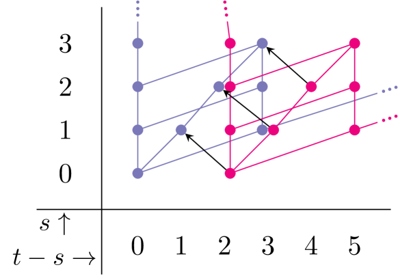
Figure 2. Left: the short exact sequence (4.70). Right: the induced long exact sequence in Ext groups. These diagrams are part of the proof of 4.69.

Compiling the information of $\mathrm{Ext}$ on (4.68) we draw the $E_{2}$-page of the Adams spectral sequence through topological degree $5$ in Figure 3.

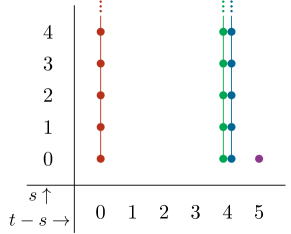
Figure 3. The $E_{2}$-page of the Adams spectral sequence computing $\Omega_{*}^{\mathrm{Spin}\text{-}\mathrm{SU}_{8}}$ .

In this range, the only differentials that could be nonzero go from the $5$-line to the $4$-line. Usually we would need to know the $6$-line in order to determine if there are any differentials from the $6$-line to the $5$-line, so that we could evaluate $\Omega_{5}^{\mathrm{Spin}\text{-}\mathrm{SU}_{8}}$, but the $5$-line is concentrated in filtration zero, and all Adams differentials land in filtration $2$ or higher, so what we have computed is good enough.

Returning to the differentials from the $5$-line to the $4$-line: Adams differentials must commute with the action of $h_{0}$ on the $E_{r}$-page, and $h_{0}$ acts by $0$ on the $5$-line but injectively on the $4$-line, so these differentials must also vanish. Thus the spectral sequence collapses giving the bordism groups in the theorem statement. The fact that $\Omega_{5}^{\mathrm{Spin}\text{-}\mathrm{SU}_{8}}\cong\mathbb{Z}/2$ is detected by $\int d$ follows from the fact that its image in the $E_{\infty}$-page is in Adams filtration zero, corresponding to Ext of the free ${\color[rgb]{0.45,0.01,0.92}\Sigma^{5}\mathcal{A}}$ summand generated by $Ud$; see [FH21a, §8.4].

∎

4.4. Determining the Manifold Generator

We now determine the generator of $\Omega_{5}^{\mathrm{Spin}\text{-}\mathrm{SU}_{8}}\cong\mathbb{Z}/2$. We start by considering a map $\widetilde{\Phi}\colon\mathrm{SU}_{2}\to\mathrm{SU}_{8}$ sending a matrix $A$ to its fourfold block sum $A\oplus A\oplus A\oplus A$. This sends $-1\mapsto-1$, so $\widetilde{\Phi}$ descends to a map

(4.73) $$\Phi\colon\mathrm{SO}_{3}=\mathrm{SU}_{2}/\{\pm 1\}\longrightarrow\mathrm{SU}_{8}/\{\pm 1\}=G_{8}.$$

Recall that $H^{*}(B\mathrm{SO}_{3};\mathbb{Z}/2)\cong\mathbb{Z}/2[w_{2},w_{3}]$ and that there are three classes $a$, $b$, and $d$ in $H^{*}(B(\mathrm{SU}_{8}/\{\pm 1\});\mathbb{Z}/2)$.

Lemma 4.74.

$\Phi^{*}(a)=w_{2}$, $\Phi^{*}(b)=w_{3}$, and $\Phi^{*}(d)=w_{2}w_{3}$.

This will imply that to find a generator, all we have to do is find a closed, oriented $5$-manifold $M$ with a principal $\mathrm{SO}_{3}$-bundle $P\to M$ with $w_{2}(M)=w_{2}(P)$ and $w_{2}(P)w_{3}(P)\neq 0$. This is easier than directly working with $G_{8}$!

Proof of 4.74.

Once we show $\Phi^{*}(a)=w_{2}$, we’re done:

(4.75a) $$\Phi^{*}(b)=\Phi^{*}(\mathrm{Sq}^{1}(a))=\mathrm{Sq}^{1}(\Phi^{*}(a))=\mathrm{Sq}^{1}(w_{2})=w_{3},$$

where the last equal sign follows by the Wu formula. In a similar way

(4.75b) $$\Phi^{*}(d)=\Phi^{*}(\mathrm{Sq}^{2}(b))=\mathrm{Sq}^{2}(\Phi^{*}(b))=\mathrm{Sq}^{2}(w_{3})=w_{2}w_{3},$$

again using the Wu formula. So all we have to do is pull back $a$.

Consider the commutative diagram of short exact sequences

(4.76)

Taking classifying spaces, this shows that the pullback of the fiber bundle $B\mathbb{Z}/2\to B\mathrm{SU}_{8}\to BG_{8}$ along the map $\Phi\colon B\mathrm{SO}_{3}\to BG_{8}$ is the fiber bundle $B\mathbb{Z}/2\to B\mathrm{SU}_{2}\to B\mathrm{SO}_{3}$. We therefore obtain a map between the Serre spectral sequences computing the mod $2$ cohomology rings of $B\mathrm{SU}_{2}$ and $B\mathrm{SU}_{8}$, and it is an isomorphism on $E_{2}^{0,*}$, i.e. on the cohomology of the fiber.

Both $B\mathrm{SU}_{2}$ and $B\mathrm{SU}_{8}$ are simply connected, so $H^{1}(\text{--};\mathbb{Z}/2)$ vanishes for both spaces. Therefore in both of these Serre spectral sequences, the generator $x$ of $E_{2}^{0,1}=H^{1}(B\mathbb{Z}/2;\mathbb{Z}/2)$ must admit a differential. The only differential that can be nonzero is the transgressing $d_{2}\colon E_{2}^{0,1}\to E_{2}^{2,0}$; in $E_{2}(\mathrm{SU}_{8})$, we saw in (4.18) that $d_{2}(x)=a$, and in $E_{2}(\mathrm{SU}_{2})$, $d_{2}(x)=w_{2}$, because $w_{2}$ is the only nonzero element of $E_{2}^{2,0}=H^{2}(B\mathrm{SO}_{3};\mathbb{Z}/2)$. Since the pullback map of spectral sequences commutes with differentials, this means $\Phi^{*}(a)=w_{2}$ as desired. ∎

Now let $W\coloneqq\mathrm{SU}_{3}/\mathrm{SO}_{3}$, which is a closed, oriented $5$-manifold called the Wu manifold, and let $P\to W$ be the quotient $\mathrm{SU}_{3}\to\mathrm{SU}_{3}/\mathrm{SO}_{3}$, which is a principal $\mathrm{SO}_{3}$-bundle. For completeness we prove the following proposition about the cohomology of the Wu manifold.

Proposition 4.77.

$H^{*}(W;\mathbb{Z}/2)\cong\mathbb{Z}/2[z_{2},z_{3}]/(z_{2}^{2},z_{3}^{2})$ with $\lvert z_{2}\rvert=2$ and $\lvert z_{3}\rvert=3$. The Steenrod squares are

(4.78) $$\mathrm{Sq}(z_{2}) =z_{2}+z_{3}$$

$$\mathrm{Sq}(z_{3}) =z_{3}+z_{2}z_{3},$$

and the Stiefel-Whitney class is $w(W)=1+z_{2}+z_{3}$. Moreover, $w(P)=1+z_{2}+z_{3}$. Thus $w_{2}(M)=w_{2}(P)$, so $W$ with $G_{8}$-bundle induced from $P$ has a spin-$\mathrm{SU}_{8}$ structure, and $w_{2}(P)w_{3}(P)\neq 0$, meaning $(W,P)$ is our sought-after generator of $\Omega_{5}^{\mathrm{Spin}\text{-}\mathrm{SU}_{8}}$.

Proof.

Once we know the cohomology ring and the Steenrod squares are as claimed, the total Stiefel-Whitney class of $W$ follows from Wu’s theorem as follows. The second Wu class $v_{2}$ is defined to be the Poincaré dual of the map

(4.79) $$x\mapsto\int_{W}\mathrm{Sq}^{2}(x)\colon H^{3}(W;\mathbb{Z}/2)\to H^{5}(W;\mathbb{Z}/2)\to\mathbb{Z}/2$$

via the Poincaré duality identification $H^{2}(W;\mathbb{Z}/2)\cong(H^{3}(W;\mathbb{Z}/2))^{\vee}$. Wu’s theorem shows that $v_{2}=w_{2}+w_{1}^{2}$, so since $H^{1}(W;\mathbb{Z}/2)=0$, $w_{1}=0$ and $w_{2}=v_{2}$. Since $\mathrm{Sq}^{2}(z_{3})=z_{2}z_{3}$, $w_{2}\neq 0$, so it must be $z_{2}$. Then $w_{3}=\mathrm{Sq}^{1}(w_{2})=z_{3}$; $w_{4}$ is trivial for degree reasons; and $w_{5}=0$ follows from the Wu formula calculating $\mathrm{Sq}^{1}(w_{4})$.

So we need to compute the cohomology ring. Consider the Serre spectral sequence for the fiber bundle

(4.80)

which has signature

(4.81) $$E_{2}^{*,*}=H^{*}(W;H^{*}(\mathrm{SO}_{3};\mathbb{Z}/2))\Longrightarrow H^{*}(\mathrm{SU}_{3};\mathbb{Z}/2).$$

A priori we must account for the action of $\pi_{1}(W)$ on $H^{*}(\mathrm{SO}_{3};\mathbb{Z}/2)$, but using the long exact sequence in homotopy groups associated to a fiber bundle one deduces that $W$ is simply connected because $\mathrm{SU}_{3}$ is; therefore we do not have to worry about this. Moreover, because $W$ is simply connected, the universal coefficient theorem tells us $H^{1}(W;\mathbb{Z}/2)=0$.

As manifolds, $\mathrm{SO}_{3}\cong\mathbb{RP}^{3}$, so $H^{*}(\mathrm{SO}_{3};\mathbb{Z}/2)\cong\mathbb{Z}/2[x]/(x^{4})$. Also, $H^{*}(\mathrm{SU}_{3};\mathbb{Z}/2)\cong\mathbb{Z}/2[c_{2},c_{3}]/(c_{2}^{2},c_{3}^{2})$, with $\lvert c_{2}\rvert=3$ and $\lvert c_{3}\rvert=5$ [Bor54, §8].

Lemma 4.82.

$H^{2}(W;\mathbb{Z}/2)\cong\mathbb{Z}/2$.

Proof.

The class $x\in E_{2}^{0,1}=H^{1}(\mathrm{SO}_{3};\mathbb{Z}/2)$ supports a differential because $H^{1}(\mathrm{SU}_{3};\mathbb{Z}/2)=0$. Since the Serre spectral sequence is first-quadrant, the only option is a transgressing $d_{2}\colon E_{2}^{0,1}\to E_{2}^{2,0}$. Therefore $\dim H^{2}(W;\mathbb{Z}/2)\geq 1$. One can also see that this is an upper bound. Since $H^{2}(\mathrm{SU}_{3};\mathbb{Z}/2)=0$ as well, any additional classes in $E_{2}^{2,0}=H^{2}(W;\mathbb{Z}/2)$ have to be killed by a differential. But the only differential that could kill those classes is the transgressing $d_{2}$ we just mentioned, and $x$ is the only nonzero element of $H^{1}(\mathrm{SO}_{3};\mathbb{Z}/2)$, so there cannot be anything else in $H^{2}(W;\mathbb{Z}/2)$. ∎

This is enough to get the cohomology ring: we already know $H^{0}$, $H^{1}$, and $H^{2}$ for the Wu manifold; Poincaré duality tells us $H^{3}(W;\mathbb{Z}/2)\cong\mathbb{Z}/2$, $H^{4}$ vanishes, and $H^{5}\cong\mathbb{Z}/2$. Therefore there must be generators $z_{2}$ and $z_{3}$ for the cohomology ring in degrees $2$ and $3$, respectively, and their squares vanish for degree reasons. And by Poincare duality $z_{2}z_{3}\neq 0$, so it is the generator of $H^{5}$. Therefore the cohomology ring is as we claimed.

Next we must determine the Steenrod squares. The fibration (4.80) pulls back from the universal $\mathrm{SO}_{3}$-bundle $\mathrm{SO}_{3}\to E\mathrm{SO}_{3}\to B\mathrm{SO}_{3}$ via the classifying map $f_{P}$ for $P$, inducing a map of Serre spectral sequences that commutes with the differentials. We draw this map in Figure 4. This map is an isomorphism on the line $E_{2}^{0,*}$, so $x\in E_{2}^{0,1}(\mathrm{SU}_{3})$ pulls back from the generator $x\in E_{2}^{0,1}(E\mathrm{SO}_{3})$ — and therefore $d_{2}(x)=z_{2}$ pulls back from a class in $E_{2}^{2,0}=H^{2}(B\mathrm{SO}_{3};\mathbb{Z}/2)$. The only nonzero class in that degree is $w_{2}$, so $f_{P}^{*}(w_{2})=z_{2}$, i.e. $w_{2}(P)=z_{2}$.

The Leibniz rule that in the Serre spectral sequence for $\mathrm{SU}_{3}$, $d_{2}(x^{2})=2xd_{2}(x)=0$. But because $H^{2}(\mathrm{SU}_{2};\mathbb{Z}/2)=0$, some differential must kill $x^{2}$. Apart from $d_{2}$, the only option is the transgressing $d_{3}\colon E_{3}^{0,2}\to E_{3}^{3,0}$, forcing $d_{3}(x^{2})=z_{3}$. A similar argument in the Serre spectral sequence for $E\mathrm{SO}_{3}$ shows that in that spectral sequence, $d_{3}(x^{2})=w_{3}$; therefore $f_{P}^{*}(w_{3})=z_{3}$ and $w_{3}(P)=z_{3}$. Pullback commutes with Steenrod squares and $\mathrm{Sq}^{1}(w_{2})=w_{3}$, so $\mathrm{Sq}^{1}(z_{2})=z_{3}$. Finally, $f_{P}^{*}(w_{2}w_{3})=z_{2}z_{3}$, and the Wu formula implies $\mathrm{Sq}^{2}(w_{3})=w_{2}w_{3}$, so $\mathrm{Sq}^{2}(z_{3})=z_{2}z_{3}$. We have computed all the Steenrod squares that could be nonzero for degree reasons, and along the way shown $w(P)=1+z_{2}+z_{3}$: the higher-degree Stiefel-Whitney classes of a principal $\mathrm{SO}_{3}$-bundle vanish. ∎

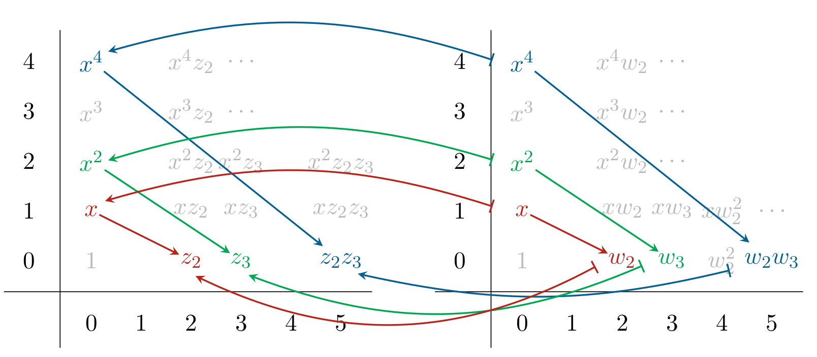
Figure 4. The fiber bundle $\mathrm{SO}_{3}\to\mathrm{SU}_{3}\to W$ pulls back from the universal $\mathrm{SO}_{3}$-bundle $\mathrm{SO}_{3}\to E\mathrm{SO}_{3}\to B\mathrm{SO}_{3}$, inducing a map of Serre spectral sequences. This map commutes with differentials and is the identity on $E_{2}^{0,\bullet}=H^{*}(\mathrm{SO}_{3};\mathbb{Z}/2)$, allowing us to conclude that ${\color[rgb]{0.72,0,0}w_{2}}$ pulls back to ${\color[rgb]{0.72,0,0}z_{2}}$, ${\color[rgb]{0,1,0}w_{3}}$ pulls back to ${\color[rgb]{0,1,0}z_{3}}$, and ${\color[rgb]{0,0.44,0.57}w_{2}w_{3}}$ pulls back to ${\color[rgb]{0,0.44,0.57}z_{2}z_{3}}$. This is a picture proof of part of 4.77.

5. Evaluating on the Anomaly

With the knowledge of the generating manifold for the $\mathbb{Z}/2$ in degree 5 as the Wu manifold, we can consider evaluating the anomaly of the theory with the field content given in §2. Since $G_{8}$ acts trivially on the scalars and the graviton only the remaining three fields could have anomalies.

Definition 5.1.

The global anomaly for a fermion on a Riemannian manifold $M$ in a a representation R coupled to background $G$ gauge field is given by an invertible field theory with partition function the exponential of an $\eta$-invariant of the Dirac operator, $\eta_{M,\textit{R}}(\mathcal{D})$[WY19, Section 4.3].

• For gauginos it is given by $\mathcal{A}_{1/2}=\exp(\pi i\eta_{M,\textit{R}}(\mathcal{D})/2)$ [Wit16, FH21a].

• For gravitinos it is given by $\mathcal{A}_{3/2}=\exp(\pi i\eta_{\text{gravitino}}/2)$ where

  (5.2) $$\eta_{\text{gravitino}}=\eta_{M,\textit{R}}(\mathcal{D}_{\text{Dirac}\times TW})-2\eta_{M,\textit{R}}(\mathcal{D})\,,$$

  and $\eta_{M,\textit{R}}(\mathcal{D}_{\text{Dirac}\times TW})$ is the Dirac operator acting on the spinor bundle tensored with the tangent bundle [HTY22].

For the remainder of the paper we will drop the $M$ subscript label.

Lemma 5.3.

If $\mathit{R}=\sum_{i}\mathit{R}_{i}$ then $\eta_{M,\,\sum_{i}\textit{R}_{i}}(\mathcal{D})=\sum_{i}\eta_{M,\,\textit{R}_{i}}(\mathcal{D})$.

The anomaly for the vector boson is not given in terms of an $\eta$-invariant, but we assume that it is also an invertible theory, and we show that it also vanishes. The next section is dedicated to showing:

Theorem 5.4.

The total anomaly (global and perturbative) of 4d $\mathcal{N}=8$ supergravity arising from the gaugino, vector boson, and gravitino, vanishes on the Wu manifold.

5.1. Evaluating on the Wu manifold

The full anomaly denoted by $\mathcal{A}$ can be written schematically as

(5.5) $$``\mathcal{A}=\mathcal{A}^{\text{pert}}_{1/2}\otimes\mathcal{A}^{\text{pert}}_{1}\otimes\mathcal{A}^{\text{pert}}_{3/2}\otimes\mathcal{A}^{\text{np}}_{1/2}\otimes\mathcal{A}^{\text{np}}_{1}\otimes\mathcal{A}^{\text{np}}_{3/2}\,"$$

where we have split up each part of the perturbative and nonperturbative anomaly coming from the gaugino, vector boson, and gravitino. Technically speaking, separating the anomaly in this way is not something that can be done canonically. By (3.4) the nontopological part arises as a quotient of the invertible theory by the topological theories. We write the anomaly in such a way in order to make it organizationally more clear. The Adams computation shows that the free part of $\Omega^{\mathrm{Spin}\text{-}\mathrm{SU}_{8}}_{6}$ is nontrivial but it was shown in [Mar85, BHN10] that in fact the entire perturbative component of the anomaly vanishes.

The vector bosons can be defined without choosing a spin structure, and therefore the partition function of their anomaly field theory factors through the quotient by fermion parity. That is, the tangential structure is

(5.6) $$\mathrm{SO}\times G_{8}=(\mathrm{Spin}\text{-}\mathrm{SU}_{8})/\{\pm 1\}\,.$$

We will proceed in understanding the perturbative anomalies by isolating $\mathcal{A}^{\text{pert}}_{1}$.

Lemma 5.7.

The perturbative anomaly for the vector bosons independently vanishes.

Proof.

With the knowledge that the manifold generator for the anomaly is the Wu manifold, we will further restrict to the $\mathrm{SO}_{3}$ inside of $G_{8}$; we are left to computing $\Omega^{\mathrm{SO}}_{6}(B\mathrm{SO}_{3})\otimes\mathbb{Q}$ , which isolates the free summand. For the degree we are after, we can compute the bordism group via the AHSS. We take the $E^{2}$ page of

(5.8) $$E_{p,q}^{2}=H_{p}(B\mathrm{SO}_{3},\Omega^{\mathrm{SO}}_{q}(\mathrm{pt}))\Longrightarrow\Omega^{\mathrm{SO}}_{6}(B\mathrm{SO}_{3})\,,$$

where

(5.9) $$\Omega_{*}^{\mathrm{SO}}(\mathrm{pt})=\{\,\mathbb{Z}\,,\,0\,,\,0\,,\,0\,,\mathbb{Z}\,,\,\mathbb{Z}/2\,,\,0\,,\ldots\,\}\,,$$

and tensor with $\mathbb{Q}$. This is equivalent to the $E_{\infty}$ page, as all differentials vanish, and is given by

(5.18) $$\begin{array}[]{c|ccccccccc}6&0\\ 5&0&0\\ 4&\mathbb{Q}&0&0&0&\mathbb{Q}&0\\ 3&0&0&0&0&0&0\\ 2&0&0&0&0&0&0\\ 1&0&0&0&0&0&0\\ 0&\mathbb{Q}&0&0&0&\mathbb{Q}&0&0\\ \hline\cr&0&1&2&3&4&5&6\end{array}$$

We see that the perturbative anomaly of the vector boson vanishes. ∎

Corollary 5.19.

The perturbative anomalies from the fractional spin particles vanish on their own.

Having established this corollary, we may now pullback the anomaly in (5.5) to the nonperturbative part, and the equation becomes literally true.

The $\eta$-invariant for the contributions in $\mathcal{A}^{\text{np}}_{1/2}\otimes\mathcal{A}^{\text{np}}_{3/2}$ is therefore a bordism invariant, and in particular the $\eta$-invariant is computed as two times some other representation and is twice another bordism invariant. In order to see this, we consider how 56, 28, and 8 split via our fourfold embedding of $\mathrm{SU}_{2}$ into $G_{8}$ for the Wu manifold. We see that 56 gives the dimension of the alternating three forms in 8-dimensions, 28 the dimension of alternating two forms, and 8 is the defining representation. The branchings are given by

(5.20) 56 $$\rightarrow 2(10\times\textbf{2}+2\times\textbf{4}),$$

(5.21) 28 $$\rightarrow 2(3\times\textbf{3}+5\times\textbf{1}),$$

(5.22) 8 $$\rightarrow 4\times\textbf{2}\,,$$

where the right hand side is in terms of $\mathfrak{su_{2}}$ representations. In increasing numerical order, they are the trivial, defining, adjoint, and $\mathrm{Sym}^{4}$ representation. To show this, notice that $\boldsymbol{8}$ splits as $V^{\oplus 4}$ when we pull back to $\mathrm{SU}_{2}$, where $V=\boldsymbol{2}$. We then consider the ways of splitting the alternating three forms. This can be done as

(5.23) $$\wedge^{2}V\otimes\wedge^{1}V\otimes\wedge^{0}V\otimes\wedge^{0}V=\mathbb{C}\otimes V\otimes\mathbb{C}\otimes\mathbb{C}\,$$

in 12 ways, essentially partitioning $3$ into a sum of length 2. The $\mathbb{C}$ for both $\wedge^{2}V$ and $\wedge^{0}V$ show that they are isomorphic as representations. It can also split into

(5.24) $$\wedge^{1}V\otimes\wedge^{1}V\otimes\wedge^{1}V\otimes\wedge^{0}V=V\otimes V\otimes V\otimes\mathbb{C}$$

in 4 ways. The fact that the third tensor product of the defining representation decomposes as $\textbf{2}\otimes\textbf{2}\otimes\textbf{2}=\textbf{2}+\textbf{2}+\textbf{4}$, gives us (5.20). Similarly, the two forms can be split into

(5.25) $$\wedge^{2}V\otimes\wedge^{0}V\otimes\wedge^{0}V\otimes\wedge^{0}V\quad\text{and}\quad\wedge^{1}V\otimes\wedge^{1}V\otimes\wedge^{0}V\otimes\wedge^{0}V$$

in 4 ways and 6 ways, respectively. The fact that $\textbf{2}\otimes\textbf{2}=\textbf{1}+\textbf{3}$, establishes (5.21).

To argue that the anomaly vanishes, we also want to show that $\eta_{\textbf{R}}(\mathcal{D}_{\text{Dirac}})$ is an integer. But since the local anomaly for the fermion vanished, the $\eta$-invariant is a bordism invariant. This can be seen from the Atiyah-Patodi-Singer (APS) index theorem, and the index for a Dirac operator makes sense on a 6-manifold. Due to the special features of the Wu-manifold, we can instead just work with representations when evaluating the anomaly. The gaugino was in the representation 56, and via the branching in (5.20), this is 4 times the $\eta$-invariant of some other representation; this implies $\mathcal{A}^{\text{np}}_{1/2}$ is zero.

As a spin 3/2 particle, the gravitino contains a spinor index as well as a Lorentz index, therefore in order to use (5.2) for the anomaly, we need to use the fact that the tangent bundle of the Wu manifold is an associated bundle.

Lemma 5.26.

The tangent bundle of the Wu manifold $W$ is given by

$$TW=\mathrm{SU}(3)\times_{\mathrm{SO}(3)}\frac{\mathfrak{su}_{3}}{\mathfrak{so}_{3}}\,.$$

Proof.

The fact that the Wu manifold is a homogeneous space allows us to use the following general procedure to construct its tangent bundle. For $H\subset G$ is a closed subgroup of a Lie group $G$, we have the following exact sequence of adjoint representations of $H$:

(5.27)

The canonical principal $H$-bundle $H\rightarrow G/H$ gives an exact functor from representations of $H$ to vector bundles over $G/H$. This gives a corresponding sequence of vector bundles:

(5.28)

There is an isomorphism $G\times_{H}\mathfrak{g/h}\rightarrow T(G/H)$ shown in [Cap19]. Let $p:G\rightarrow G/H$ and $L_{X}$ be the left invariant vector field generated by $X\in\mathfrak{h}$. Then the mapping of $(g,X+\mathfrak{h})\in G\times(\mathfrak{g/h})$ to $T_{g}p\cdot L_{X}(g)\in T_{gH}(G/H)$ gives the isomorphism. Specifically for our problem, we have the $\mathrm{SO}_{3}$-bundle $\mathrm{SU}_{3}\rightarrow W$, which by the present construction gives the desired result. ∎

Remark 5.29.

This is an example of the “mixing construction”: for a principal $G$-bundle $P\rightarrow M$ and a $G$-representation $V$, the space $P\times_{G}V$ is a vector bundle over $M$ with rank equal to the dimension of $V$.

We are now left to understand $\frac{\mathfrak{su}_{3}}{\mathfrak{so}_{3}}$ as a representation of $\mathrm{SO}_{3}$. The Lie algebra $\mathfrak{su}_{3}$ is an $\mathrm{SU}_{3}$-representation, and restricting, it is also an $\mathrm{SO}_{3}$ representation of dimension 8. But the $\mathbf{8}$ of $\mathfrak{su}_{3}$ branches as $\mathbf{8}\rightarrow\mathbf{1}+\mathbf{1}+\mathbf{3}+\mathbf{3}$ in $\mathfrak{so}_{3}$, so quotienting by $\mathfrak{so}_{3}$ then eliminates one of the 3 summands. Then $\eta(\mathcal{D}_{\text{Dirac}\times TW})=(\mathbf{1}+\mathbf{1}+\mathbf{3})\,\eta(\mathcal{D}_{\text{Dirac}})$, which means the gravitino contributes 3$\eta(\mathcal{D}_{\text{Dirac}})$. By the branching in (5.22), $\eta(\mathcal{D}_{\text{Dirac}})$ of 8 in $\mathfrak{su}_{8}$ is determined by 2 of $\mathfrak{su}_{2}$, and using Lemma 5.3, we have a multiple of 4 worth of $\eta_{\textbf{2}}(\mathcal{D}_{\text{Dirac}})$ and that determines $\eta_{\text{gravitino}}$. Then the anomaly $\mathcal{A}^{\text{np}}_{3/2}$ associated to $\eta_{\text{gravitino}}$ vanishes per the above discussion for the gauginos.

We now move onto the nonperturbative anomaly from the vector bosons, which is accessible from $\Omega^{\mathrm{SO}}_{5}(B\mathrm{SO}_{3})$. By applying (5.9) to the AHSS, we only need to consider $H_{5}(B\mathrm{SO}_{3},\mathbb{Z})$ as well as the $\mathbb{Z}/2$ element in bidegree $(0,5)$. One can evaluate the torsion part of $H_{5}(B\mathrm{SO}_{3};\mathbb{Z})$ by the universal coefficient theorem, and looking at $H^{6}(B\mathrm{SO}_{3};\mathbb{Z})$. We find that this is given by $w_{2}w_{3}$ of the $\mathrm{SO}_{3}$ bundle and is nontrivial on the Wu manifold. Then the AHSS says $\Omega_{5}^{\mathrm{SO}}(B\mathrm{SO}_{3})=\mathbb{Z}/2\times\mathbb{Z}/2$ detected by the bordism invariants $\int w_{2}(TM)w_{3}(TM)$ and $\int w_{2}(P)w_{3}(P)$; these are generated by $W$ with trivial bundle, and $W$ with the principal $\mathrm{SO}_{3}$-bundle. We see that while the bosonic anomaly is in principle $\mathbb{Z}/2\times\mathbb{Z}/2$ valued, and coupling to spin structure eliminates one of the $\mathbb{Z}/2$. Using (5.21), for the representation of the vector boson, the anomaly is also twice of something as a bordism invariant. This is reasonable since the anomaly of multiple particles is the tensor product of their anomalies . The anomaly for the vector bosons is 2 times something as a bordism invariant, since the perturbative part vanished, and considering that we have argued that everything else in (5.5) vanishes aside from $\mathcal{A}^{\text{np}}_{1}$, we have that $\mathcal{A}=\mathcal{A}^{\text{np}}_{1}$. But $\mathcal{A}$ is $\mathbb{Z}/2$ valued, and with $\mathcal{A}^{\text{np}}_{1}$ equating to 0 mod 2, the full anomaly vanishes, thus establishing proposition 5.4.

References

- [Ada21] Katharine L. M. Adamyk. Classifying and extending -local -modules. 2021. https://arxiv.org/abs/2107.02837.
- [Ada58] J.F. Adams. On the structure and applications of the Steenrod algebra. Commentarii mathematici Helvetici, 32:180–214, 1957/58.
- [And69] D.W. Anderson. Universal coefficient theorems for -theory. 1969. https://faculty.tcu.edu/gfriedman/notes/Anderson-UCT.pdf.
- [Ave59] B. G. Averbuh. Algebraic structure of cobordism groups. Dokl. Akad. Nauk SSSR, 125:11–14, 1959.
- [BB65] Paul F. Baum and William Browder. The cohomology of quotients of classical groups. Topology, 3(4):305–336, June 1965.
- [BC18] Agnès Beaudry and Jonathan A. Campbell. A guide for computing stable homotopy groups. In Topology and quantum theory in interaction, volume 718 of Contemp. Math., pages 89–136. Amer. Math. Soc., [Providence], RI, [2018] ©2018. https://arxiv.org/abs/1801.07530.
- [BHN10] Guillaume Bossard, Christian Hillmann, and Hermann Nicolai. symmetry in perturbatively quantised supergravity. JHEP, (52), 2010. https://arxiv.org/abs/1007.5472.
- [BLT20] Lakshya Bhardwaj, Yasunori Lee, and Yuji Tachikawa. action on QFTs with symmetry and the Brown-Kervaire invariants. Journal of High Energy Physics, 2020(141), 2020. https://arxiv.org/abs/2009.10099.
- [Bor51] Armand Borel. Sur la cohomologie des espaces homogènes des groupes de Lie compacts. C. R. Acad. Sci. Paris, 233:569–571, 1951.
- [Bor53] Armand Borel. Sur la cohomologie des espaces fibrés principaux et des espaces homogènes de groupes de Lie compacts. Ann. of Math. (2), 57:115–207, 1953.
- [Bor54] Armand Borel. Sur l’homologie et la cohomologie des groupes de Lie compacts connexes. Amer. J. Math., 76:273–342, 1954.
- [Cam17] Jonathan A. Campbell. Homotopy theoretic classification of symmetry protected phases. 2017. https://arxiv.org/abs/1708.04264.
- [Cap19] Andreas Cap. Geometry of homogeneous spaces. 2019. https://www.mat.univie.ac.at/~cap/files/Geom-Homog.pdf.
- [Car14] Élie Cartan. Les groupes réels simples, finis et continus. Ann. Sci. École Norm. Sup. (3), 31:263–355, 1914.
- [CJ79] E. Cremmer and B. Julia. The supergravity. Nuclear Phys. B, 159(1-2):141–212, 1979.
- [DDHM22] Arun Debray, Markus Dierigl, Jonathan J. Heckman, and Miguel Montero. The anomaly that was not meant IIB. Fortschr. Phys., 70(1):Paper No. 2100168, 31, 2022. https://arxiv.org/abs/2107.14227.
- [Deb22] Arun Debray. The 2-group symmetries of the heterotic and CHL strings. 2022. To appear.
- [DGG21] Diego Delmastro, Davide Gaiotto, and Jaume Gomis. Global anomalies on the Hilbert space. Journal of High Energy Physics, 2021(142), 2021. https://arxiv.org/abs/2101.02218.
- [DGL20] Joe Davighi, Ben Gripaios, and Nakarin Lohitsiri. Global anomalies in the standard model(s) and beyond. J. High Energy Phys., (7):232, 50, 2020. https://arxiv.org/abs/1910.11277.
- [DGL22] Joe Davighi, Ben Gripaios, and Nakarin Lohitsiri. Anomalies of non-Abelian finite groups via cobordism. J. High Energy Phys., (9):Paper No. 147, 2022. https://arxiv.org/abs/2207.10700.
- [DL20] Joe Davighi and Nakarin Lohitsiri. Anomaly interplay in gauge theories. J. High Energy Phys., (5):098, 20, 2020. https://arxiv.org/abs/2001.07731.
- [DL21a] Joe Davighi and Nakarin Lohitsiri. Omega vs. pi, and 6d anomaly cancellation. Journal of High Energy Physics, 2021(267), 2021. https://arxiv.org/abs/2012.11693.
- [DL21b] Joe Davighi and Nakarin Lohitsiri. The algebra of anomaly interplay. SciPost Phys., 10(3):074, 2021. https://arxiv.org/abs/2011.10102.
- [DY23] Arun Debray and Matthew Yu. T-Duality Bordism. To Appear, 2023.
- [FH21a] Daniel S. Freed and Michael J. Hopkins. Consistency of M-theory on non-orientable manifolds. Q. J. Math., 72(1-2):603–671, 2021. https://arxiv.org/abs/1908.09916.
- [FH21b] Daniel S. Freed and Michael J. Hopkins. Reflection positivity and invertible topological phases. Geom. Topol., 25(3):1165–1330, 2021. https://arxiv.org/abs/1604.06527.
- [FHT10] Daniel S. Freed, Michael J. Hopkins, and Constantin Teleman. Consistent orientation of moduli spaces. In The many facets of geometry, pages 395–419. Oxford Univ. Press, Oxford, 2010.
- [FM06] Daniel S. Freed and Gregory W. Moore. Setting the quantum integrand of M-theory. Comm. Math. Phys., 263(1):89–132, 2006. https://arxiv.org/abs/hep-th/0409135.
- [FM13] Sergio Ferrara and Alessio Marrani. Quantum gravity needs supersymmetry. In Antonino Zichichi, editor, Searching for the Unexpected at LHC and the Status of Our Knowledge, volume 49 of The Subnuclear Series, pages 53–67, 2013. https://arxiv.org/abs/1201.4328.
- [Fre14] Daniel S. Freed. Anomalies and Invertible Field Theories. Proc. Symp. Pure Math., 88:25–46, 2014. https://arxiv.org/abs/1404.7224.
- [Fre19] Daniel S. Freed. Lectures on field theory and topology, volume 133 of CBMS Regional Conference Series in Mathematics. American Mathematical Society, Providence, RI, 2019. Published for the Conference Board of the Mathematical Sciences.
- [FT14] Daniel S. Freed and Constantin Teleman. Relative quantum field theory. Comm. Math. Phys., 326(2):459–476, 2014. https://arxiv.org/abs/1212.1692.
- [GEM19] Iñaki García-Etxebarria and Miguel Montero. Dai-Freed anomalies in particle physics. JHEP, 08:003, 2019. https://arxiv.org/abs/1808.00009.
- [GOP+20] Meng Guo, Kantaro Ohmori, Pavel Putrov, Zheyan Wan, and Juven Wang. Fermionic finite-group gauge theories and interacting symmetric/crystalline orders via cobordisms. Comm. Math. Phys., 376(2):1073–1154, 2020. https://arxiv.org/abs/1812.11959.
- [GP21a] Daniel Grady and Dmitri Pavlov. The geometric cobordism hypothesis. 2021. https://arxiv.org/abs/2111.01095.
- [GP21b] Andrea Grigoletto and Pavel Putrov. Spin-cobordisms, surgeries and fermionic modular bootstrap. 2021. https://arxiv.org/abs/2106.16247.
- [GPW18] Meng Guo, Pavel Putrov, and Juven Wang. Time reversal, Yang-Mills and cobordisms: Interacting topological superconductors/insulators and quantum spin liquids in 3+1d. Annals of Physics, 394:244–293, 2018. https://arxiv.org/abs/1711.11587.
- [Gri21] Andrea Grigoletto. Anomalies of fermionic cfts via cobordism and bootstrap. 2021. https://arxiv.org/abs/2112.01485.
- [HKT20] Itamar Hason, Zohar Komargodski, and Ryan Thorngren. Anomaly Matching in the Symmetry Broken Phase: Domain Walls, CPT, and the Smith Isomorphism. SciPost Phys., 8:62, 2020. https://arxiv.org/abs/1910.14039.
- [Hsi18] Chang-Tse Hsieh. Discrete gauge anomalies revisited. 2018. https://arxiv.org/abs/1808.02881.
- [HTY22] Chang-Tse Hsieh, Yuji Tachikawa, and Kazuya Yonekura. Anomaly inflow and -form gauge theories. Comm. Math. Phys., 391(2):495–608, 2022. https://arxiv.org/abs/2003.11550.
- [Iwa49] Kenkichi Iwasawa. On some types of topological groups. Ann. of Math. (2), 50:507–558, 1949.
- [JF20] Theo Johnson-Freyd. Topological Mathieu moonshine. 2020. https://arxiv.org/abs/2006.02922.
- [Kil88] T. P. Killingback. Global anomalies, string theory and spacetime topology. Classical Quantum Gravity, 5(9):1169–1185, 1988. With an appendix by W. Rose.
- [Koi21] Saki Koizumi. Global anomalies and bordism invariants in one dimension. 2021. https://arxiv.org/abs/2111.15254.
- [KPMT20] Justin Kaidi, Julio Parra-Martinez, and Yuji Tachikawa. Topological superconductors on superstring worldsheets. SciPost Phys., 9(1):Paper No. 010, 70, 2020. With a mathematical appendix by Arun Debray. https://arxiv.org/abs/1911.11780.
- [Kud56] Tatsuji Kudo. A transgression theorem. Mem. Fac. Sci. Kyūsyū Univ. A, 9:79–81, 1956.
- [Las63] R. Lashof. Poincaré duality and cobordism. Trans. Amer. Math. Soc., 109:257–277, 1963.
- [LOT21a] Yasunori Lee, Kantaro Ohmori, and Yuji Tachikawa. Matching higher symmetries across Intriligator-Seiberg duality. Journal of High Energy Physics, 2021(114), 2021. https://arxiv.org/abs/2108.05369.
- [LOT21b] Yasunori Lee, Kantaro Ohmori, and Yuji Tachikawa. Revisiting Wess-Zumino-Witten terms. SciPost Phys., 10:61, 2021. https://arxiv.org/abs/2009.00033.
- [LT21] Yasunori Lee and Yuji Tachikawa. Some comments on 6D global gauge anomalies. PTEP, 2021(8):08B103, 2021. https://arxiv.org/abs/2012.11622.
- [LY22] Yasunori Lee and Kazuya Yonekura. Global anomalies in 8d supergravity. J. High Energy Phys., (7):Paper No. 125, 2022. https://arxiv.org/abs/2203.12631.
- [Mal45] A. Malcev. On the theory of the Lie groups in the large. Rec. Math. [Mat. Sbornik] N. S., 16(58):163–190, 1945.
- [Mar85] Neil Marcus. Composite anomalies in supergravity. Phys. Lett. B, 157(5-6):383–388, 1985.
- [MCB22] Naren Manjunath, Vladimir Calvera, and Maissam Barkeshli. Non-perturbative constraints from symmetry and chirality on Majorana zero modes and defect quantum numbers in (2+1)D. 2022. https://arxiv.org/abs/2210.02452.
- [Mil60] J. Milnor. On the cobordism ring and a complex analogue. I. Amer. J. Math., 82:505–521, 1960.
- [MM19] Samuel Monnier and Gregory W. Moore. Remarks on the Green-Schwarz terms of six-dimensional supergravity theories. Comm. Math. Phys., 372(3):963–1025, 2019. https://arxiv.org/abs/1808.01334.
- [Mon15] Samuel Monnier. Global gravitational anomaly cancellation for five-branes. Advances in Theoretical and Mathematical Physics, 19(3):701–724, 2015. https://arxiv.org/abs/1310.2250.
- [Mon17] Samuel Monnier. The anomaly field theories of six-dimensional (2,0) superconformal theories. 2017. https://arxiv.org/abs/1706.01903.
- [PS16] T. Pantev and E. Sharpe. Duality group actions on fermions. JHEP, 11:171, 2016. https://arxiv.org/abs/1609.00011.
- [Ser53] Jean-Pierre Serre. Cohomologie modulo des complexes d’Eilenberg-MacLane. Comment. Math. Helv., 27:198–232, 1953.
- [SP18] Christopher J. Schommer-Pries. Tori detect invertibility of topological field theories. Geom. Topol., 22(5):2713–2756, 2018. https://arxiv.org/abs/1511.01772.
- [Spe22] David E Speyer. Is there a representation of that doesn’t lift to a spin group?, 2022. MathOverflow answer. https://mathoverflow.net/q/430180.
- [STY18] Nathan Seiberg, Yuji Tachikawa, and Kazuya Yonekura. Anomalies of duality groups and extended conformal manifolds. PTEP. Prog. Theor. Exp. Phys., (7):073B04, 27, 2018. https://arxiv.org/abs/1803.07366.
- [Tac22] Yuji Tachikawa. Topological modular forms and the absence of a heterotic global anomaly. PTEP. Prog. Theor. Exp. Phys., (4):Paper No. 04A107, 8, 2022. https://arxiv.org/abs/2103.12211.
- [Tho20] Ryan Thorngren. Anomalies and bosonization. Comm. Math. Phys., 378(3):1775–1816, 2020. https://arxiv.org/abs/1810.04414.
- [Tod87] Hiroshi Toda. Cohomology of classifying spaces. In Homotopy theory and related topics, pages 75–108. Mathematical Society of Japan, 1987.
- [TY19] Yuji Tachikawa and Kazuya Yonekura. Why are fractional charges of orientifolds compatible with Dirac quantization? SciPost Phys., 7:58, 2019. https://arxiv.org/abs/1805.02772.
- [TY21] Yuji Tachikawa and Mayuko Yamashita. Topological modular forms and the absence of all heterotic global anomalies. 2021. https://arxiv.org/abs/2108.13542.
- [Wit86] Edward Witten. Topological tools in ten-dimensional physics. In Workshop on unified string theories (Santa Barbara, Calif., 1985), pages 400–429. World Sci. Publishing, Singapore, 1986. With an appendix by R. E. Stong.
- [Wit16] Edward Witten. Fermion Path Integrals And Topological Phases. Rev. Mod. Phys., 88(3):035001, 2016. https://arxiv.org/abs/1508.04715.
- [WNC21] Qing-Rui Wang, Shang-Qiang Ning, and Meng Cheng. Domain wall decorations, anomalies and spectral sequences in bosonic topological phases. 2021. https://arxiv.org/abs/2104.13233.
- [WW19a] Zheyan Wan and Juven Wang. Adjoint , deconfined critical phenomena, symmetry-enriched topological quantum field theory, and higher symmetry extension. Phys. Rev. D, 99:065013, Mar 2019. https://arxiv.org/abs/1812.11955.
- [WW19b] Zheyan Wan and Juven Wang. Higher anomalies, higher symmetries, and cobordisms I: classification of higher-symmetry-protected topological states and their boundary fermionic/bosonic anomalies via a generalized cobordism theory. Annals of Mathematical Sciences and Applications, 4:107–311, 2019. https://arxiv.org/abs/1812.11967.
- [WW20a] Zheyan Wan and Juven Wang. Beyond standard models and grand unifications: anomalies, topological terms, and dynamical constraints via cobordisms. J. High Energy Phys., (7):062, 90, 2020. https://arxiv.org/abs/1910.14668.
- [WW20b] Zheyan Wan and Juven Wang. Higher anomalies, higher symmetries, and cobordisms III: QCD matter phases anew. Nuclear Physics B, page 115016, 2020. https://arxiv.org/abs/1912.13514.
- [WW20c] Juven Wang and Xiao-Gang Wen. Nonperturbative definition of the standard models. Phys. Rev. Research, 2:023356, Jun 2020. https://arxiv.org/abs/1809.11171.
- [WWW19] Juven Wang, Xiao-Gang Wen, and Edward Witten. A new anomaly. J. Math. Phys., 60(5):052301, 23, 2019. https://arxiv.org/abs/1810.00844.
- [WWZ20] Zheyan Wan, Juven Wang, and Yunqin Zheng. Higher anomalies, higher symmetries, and cobordisms II: Lorentz symmetry extension and enriched bosonic/fermionic quantum gauge theory. Ann. Math. Sci. Appl., 5(2):171–257, 2020. https://arxiv.org/abs/1912.13504.
- [WY19] Edward Witten and Kazuya Yonekura. Anomaly Inflow and the -Invariant. In The Shoucheng Zhang Memorial Workshop, 9 2019. https://arxiv.org/abs/1909.08775.
- [Yam21] Mayuko Yamashita. Differential models for the Anderson dual to bordism theories and invertible QFT’s, II. 2021. https://arxiv.org/abs/2110.14828.
- [Yon22] Kazuya Yonekura. Heterotic global anomalies and torsion Witten index. 2022. https://arxiv.org/abs/2207.13858.
- [Yos75] Zen-ichi Yosimura. Universal coefficient sequences for cohomology theories of CW-spectra. Osaka J. Math., 12(2):305–323, 1975.
- [Yu21] Matthew Yu. Symmetries and anomalies of (1+1)d theories: 2-groups and symmetry fractionalization. JHEP, 08:061, 2021. https://arxiv.org/abs/2010.01136.
- [Yu22] Matthew Yu. Genus-one data and anomaly detection. Phys. Rev. D, 105(10):106007, 2022.
- [YY21] Mayuko Yamashita and Kazuya Yonekura. Differential models for the Anderson dual to bordism theories and invertible QFT’s, I. 6 2021. https://arxiv.org/abs/2106.09270.