Certified Training:
Small Boxes are All You Need
Abstract
To obtain, deterministic guarantees of adversarial robustness, specialized training methods are used. We propose, SABR, a novel such certified training method, based on the key insight that propagating interval bounds for a small but carefully selected subset of the adversarial input region is sufficient to approximate the worst-case loss over the whole region while significantly reducing approximation errors. We show in an extensive empirical evaluation that SABR outperforms existing certified defenses in terms of both standard and certifiable accuracies across perturbation magnitudes and datasets, pointing to a new class of certified training methods promising to alleviate the robustness-accuracy trade-off.
1 Introduction
As neural networks are increasingly deployed in safety-critical domains, formal robustness guarantees against adversarial examples (Biggio et al., 2013; Szegedy et al., 2014) are becoming ever more important. However, despite significant progress, specialized training methods that improve certifiability at the cost of severely reduced accuracies are still required to obtain deterministic guarantees.
Given an input region defined by an adversary specification, both training and certification methods compute a network’s reachable set by propagating a symbolic over-approximation of this region through the network (Singh et al., 2018; 2019a; Gowal et al., 2018a). Depending on the propagation method, both the computational complexity and approximation-tightness can vary widely. For certified training, an over-approximation of the worst-case loss is computed from this reachable set and then optimized (Mirman et al., 2018; Wong et al., 2018). Surprisingly, the least precise propagation methods yield the highest certified accuracies as more precise methods induce harder optimization problems (Jovanovic et al., 2021). However, the large approximation errors incurred by these imprecise methods lead to over-regularization and thus poor accuracy. Combining precise worst-case loss approximations and a tractable optimization problem is thus the core challenge of certified training.
In this work, we tackle this challenge and propose a novel certified training method, SABR, Small Adversarial Bounding Regions, based on the following key insight: by propagating small but carefully selected subsets of the adversarial input region with imprecise methods (i.e., Box), we can obtain both well-behaved optimization problems and precise approximations of the worst-case loss. This yields less over-regularized networks, allowing SABR to improve on state-of-the-art certified defenses in terms of both standard and certified accuracies across settings, thereby pointing to a new class of certified training methods.
Main Contributions
Our main contributions are:
-
•
A novel certified training method, SABR, reducing over-regularization to improve both standard and certified accuracy (Section 3).
-
•
A theoretical investigation motivating SABR by deriving new insights into the growth of Box relaxations during propagation (Section 4).
-
•
An extensive empirical evaluation demonstrating that SABR outperforms all state-of-the-art certified training methods in terms of both standard and certifiable accuracies on MNIST, CIFAR-10, and TinyImageNet (Section 5).
2 Background
In this section, we provide the necessary background for SABR.
Adversarial Robustness
Consider a classification model that, given an input , predicts numerical scores for every class. We say that is adversarially robust on an -norm ball of radius if it consistently predicts the target class for all perturbed inputs . More formally, we define adversarial robustness as:
| (1) |
Neural Network Verification
To verify that a neural network is adversarially robust, several verification techniques have been proposed.
A simple but effective such method is verification with the Box relaxation (Mirman et al., 2018), also called interval bound propagation (IBP) (Gowal et al., 2018b). Conceptually, we first compute an over-approximation of a network’s reachable set by propagating the input region through the neural network and then check whether all outputs in the reachable set yield the correct classification. This propagation sequentially computes a hyper-box (each dimension is described as an interval) relaxation of a layer’s output, given a hyper-box input. As an example, consider an -layer network , with linear layers and ReLU activation functions . Given an input region , we over-approximate it as a hyper-box, centered at and with radius , such that we have the th dimension of the input . Given a linear layer , we obtain the hyper-box relaxation of its output with centre and radius , where denotes the elementwise absolute value. A ReLU activation can be over-approximated by propagating the lower and upper bound separately, resulting in a output hyper-box with and where and . Proceeding this way for all layers, we obtain lower and upper bounds on the network output and can check if the output score of the target class is greater than that of all other classes by computing the upper bound on the logit difference and then checking whether .
We illustrate this propagation process for a one-layer network in Fig. 1. There, the blue shapes ( ) show an exact propagation of the input region and the red shapes ( ) their hyper-box relaxation. Note how after the first linear and ReLU layer (third row), the relaxation (red) contains already many points not reachable via exact propagation (blue), despite it being the smallest hyper-box containing the exact region. These so-called approximation errors accumulate quickly, leading to an increasingly imprecise abstraction, as can be seen by comparing the two shapes after an additional linear layer (last row). To verify that this network classifies all inputs in to class , we have to show the upper bound of the logit difference to be less than . While the concrete maximum of (black ) is indeed less than , showing that the network is robust, the Box relaxation only yields (red ) and is thus too imprecise to prove it.
Beyond Box, more precise verification approaches track more relational information at the cost of increased computational complexity (Palma et al., 2022; Wang et al., 2021). A recent example is MN-BaB (Ferrari et al., 2022), which improves on Box in two key ways: First, instead of propagating axis-aligned hyper-boxes, it uses much more expressive polyhedra, allowing linear layers to be captured exactly and ReLU layers much more precisely. Second, if the result is still too imprecise, the verification problem is recursively split into easier ones, by introducing a case distinction between the two linear segments of the ReLU function. This is called the branch-and-bound (BaB) approach (Bunel et al., 2020). We refer the interested reader to Ferrari et al. (2022) for more details.
Training for Robustness
For neural networks to be certifiably robust, special training is necessary. Given a data distribution , standard training generally aims to find a network parametrization that minimizes the expected cross-entropy loss (see Section B.1):
| (2) |
When training for robustness, we, instead, wish to minimize the expected worst-case loss around the data distribution, leading to the min-max optimization problem:
| (3) |
Unfortunately, solving the inner maximization problem is generally intractable. Therefore, it is commonly under- or over-approximated, yielding adversarial and certified training, respectively. For notational clarity, we henceforth drop the subscript .
Adversarial Training
Adversarial training optimizes a lower bound on the inner optimization objective in Eq. 3 by first computing concrete examples maximizing the loss term and then optimizing the network parameters for these samples. Typically, is computed by initializing uniformly at random in and then updating it over projected gradient descent steps (PGD) (Madry et al., 2018) , with step size and projection operator . While networks trained this way typically exhibit good empirical robustness, they remain hard to formally verify and sometimes vulnerable to stronger or different attacks (Tramèr et al., 2020; Croce & Hein, 2020).
Certified Training
Certified training optimizes an upper bound on the inner maximization objective in Eq. 3, obtained via a bound propagation method. These methods compute an upper bound on the logit differences , as described above, to obtain the robust cross-entropy loss . We will use Box to refer to the verification and propagation approach, and IBP to refer to the corresponding training method.
Surprisingly, using the imprecise Box relaxation (Mirman et al., 2018; Gowal et al., 2018b; Shi et al., 2021) consistently produces better results than methods based on tighter abstractions (Zhang et al., 2020; Balunovic & Vechev, 2020; Wong et al., 2018). Jovanovic et al. (2021) trace this back to the optimization problems induced by the more precise methods becoming intractable to solve. While the heavily regularized, IBP trained networks are amenable to certification, they suffer from severely reduced (standard) accuracies. Overcoming this robustness-accuracy trade-off remains a key challenge of robust machine learning.
3 Method – Small Regions for Certified Training
To train networks that are not only robust and amenable to certification but also retain comparatively high standard accuracies, we propose the novel certified training method, SABR — Small Adversarial Bounding Regions. We leverage the key insight that computing an over-approximation of the worst-case loss over a small but carefully selected subset of the input region often yields a good proxy for the worst-case loss over the whole region while significantly reducing approximation errors.
We illustrate this intuition in Fig. 2. Existing certified training methods always consider the whole input region (dashed box in the input panel). Propagating such large regions through the network yields quickly growing approximation errors and thus very imprecise over-approximations of the actual worst-case loss (compare the reachable set in red and green to the dashed box in the output panel), causing significant over-regularization (large blue arrow ). Adversarial training methods, in contrast, only consider individual points in the input space ( in Fig. 2) and often fail to capture the actual worst-case loss. This leads to insufficient regularization (small blue arrow in the output panel) and yields networks which are not amenable to certification and potentially not robust.
We tackle this problem by propagating small, adversarially chosen subsets of the input region (solid box in the input panel of Fig. 2), which we call the propagation region. This leads to significantly reduced approximation errors (see the solid box in the output panel) inducing a level of regularization in-between certified and adversarial training methods (medium blue arrow ), allowing us to train networks that are both robust and accurate.
More formally, we define an auxiliary objective for the robust optimization problem Eq. 3 as
| (4) |
where we replace the maximum over the whole input region with that over a carefully selected subset . While choosing would recover the original robust training problem (Eq. 3), both, computing the maximum loss over a given input region (Eq. 4) and finding a point that realizes this loss is generally intractable. Instead, we instantiate SABR by combining different approximate approaches for the two key components: a) a method for choosing the location and size of the propagation region, and b) a method used for propagating the thus selected region. Note that we thus generally do not obtain a sound over-approximation of the loss on . Depending on the size of the propagated region , SABR can be seen as a continuous interpolation between adversarial training for infinitesimally small regions and standard certified training for the full input region .
Selecting the Propagation Region
SABR aims to find and propagate a small subset of the adversarial input region that contains the inputs leading to the worst-case loss. To this end, we parametrize this propagation region as an -norm ball with centre and radius . We first choose by scaling the original perturbation radius with the subselection ratio . We then select as follows: We conduct a PGD attack, choosing the preliminary centre as the sample with the highest loss. We then ensure the obtained region is fully contained in the original one by projecting onto to obtain . We show this in Fig. 3.
Propagation Method
Having found the propagation region , we can use any symbolic propagation method to compute an over-approximation of its worst-case loss. We chose Box propagation (DiffAI Mirman et al. (2018) or IBP (Gowal et al., 2018b)) to obtain well-behaved optimization problems (Jovanovic et al., 2021). There, choosing small propagation regions (), can significantly reduce the incurred over-approximation errors, as we will show later (see Section 4).
4 Understanding SABR: Robust Loss and Growth of Small Boxes
In this section, we aim to uncover the reasons behind SABR’s success. Towards this, we first analyse the relationship between robust loss and over-approximation size before investigating the growth of the Box approximation with propagation region size.
Robust Loss Analysis
Certified training typically optimizes an over-approximation of the worst-case cross-entropy loss , computed via the softmax of the upper-bound on the logit differences . When training with the Box relaxation and assuming the target class , w.l.o.g., we obtain the logit difference and thus the robust cross entropy loss
| (5) |
We observe that samples with high () worst-case misclassification margin dominate the overall loss and permit the per-sample loss term to be approximated as
| (6) |
Further, we note that the Box relaxations of many functions preserve the box centres, i.e., . Only unstable ReLUs, i.e., ReLUs containing in their input bounds, introduce a slight shift. However, these are empirically few in certifiably trained networks (see Table 4).
These observations allow us to decompose the robust loss into an accuracy term , corresponding to the misclassification margin of the adversarial example at the centre of the propagation region, and a robustness term , bounding the difference to the actual worst-case loss. These terms generally represent conflicting objectives, as local robustness requires the network to disregard high frequency features (Ilyas et al., 2019). Therefore, robustness and accuracy are balanced to minimize the optimization objective Eq. 5. Consequently, reducing the regularization induced by the robustness term will bias the optimization process towards standard accuracy. Next, we investigate how SABR reduces exactly this regularization strength, by propagating smaller regions.
Box Growth
To investigate how Box approximations grow as they are propagated, let us again consider an -layer network , with linear layers and ReLU activation functions . Given a Box input with radius and centre distribution , we now define the per-layer growth rate as the ratio of input and expected output radius:
| (7) |
For linear layers with weight matrix , we obtain an output radius and thus a constant growth rate , corresponding to the row-wise norm of the weight matrix . Empirically, we find most linear and convolutional layers to exhibit growth rates between and (see Table 9 in Section D.4).
For ReLU layers , computing the growth rate is more challenging, as it depends on the location and size of the inputs. Shi et al. (2021) assume the input Box centres to be symmetrically distributed around , i.e., , and obtain a constant growth rate of . While this assumption holds at initialization, we observe that trained networks tend to have more inactive than active ReLUs (see Table 4), indicating asymmetric distributions with more negative inputs (see Fig. 5).
We now investigate this more realistic setting. We first consider the two limit cases where input radii go against and . When input radii are , active neurons will stay stably active, yielding and inactive neurons will stay stably inactive, yielding . Thus, we obtain a growth rate, equivalent to the portion of active neurons. In the other extreme , all neurons will become unstable with , yielding , and thus a constant growth rate of . To analyze the behavior in between those extremes, we assume pointwise asymmetry favouring negative inputs, i.e., . In this setting, we find that output radii grow strictly super-linear in the input size:
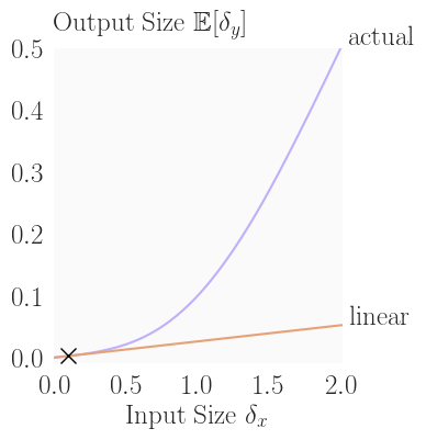
Theorem 4.1 (Hyper-Box Growth).
Let be a ReLU function and consider box inputs with radius and asymmetrically distributed centres such that . Then, the mean output radius will grow super-linearly in the input radius . More formally:
| (8) |
We defer a proof to App. A and illustrate this behaviour in Fig. 5 for the box centre distribution . There, we clearly observe that the actual super-linear growth (purple) outpaces a linear approximation (orange). While even the qualitative behaviour depends on the exact centre distribution and the input box size , we can solve special cases analytically. For example, a piecewise uniform centre distribution yields quadratic growth on its support (see App. A).
Multiplying all layer-wise growth rates, we obtain the overall growth rate , which is exponential in network depth and super-linear in input radius. When not specifically training with the Box relaxation, we empirically observe that the large growth factors of linear layers dominate the shrinking effect of the ReLU layers, leading to a quick exponential growth in network depth. Further, for both SABR and IBP trained networks, the super-linear growth in input radius empirically manifests as exponential behaviour (see Figs. 8 and 9). Using SABR, we thus expect the regularization induced by the robustness term to decrease super-linearly, and empirically even exponentially, with subselection ratio , explaining the significantly higher accuracies compared to IBP.
5 Evaluation
In this section, we first compare SABR to existing certified training methods before investigating its behavior in an ablation study.
Experimental Setup
We implement SABR in PyTorch (Paszke et al., 2019)111Code released at https://github.com/eth-sri/sabr and use MN-BaB (Ferrari et al., 2022) for certification. We conduct experiments on MNIST (LeCun et al., 2010), CIFAR-10 (Krizhevsky et al., 2009), and TinyImageNet (Le & Yang, 2015) for the challenging perturbations, using the same 7-layer convolutional architecture CNN7 as prior work (Shi et al., 2021) unless indicated otherwise (see App. C for more details). We choose similar training hyper-parameters as prior work (Shi et al., 2021) and provide more detailed information in App. C.
5.1 Main Results
We compare SABR to state-of-the-art certified training methods in Table 1 and Fig. 6, reporting the best results achieved with a given method on any architecture.
In Fig. 6, we show certified over standard accuracy (upper right-hand corner is best) and observe that SABR ( ) dominates all other methods, achieving both the highest certified and standard accuracy across all settings. As existing methods typically perform well either at large or small perturbation radii (see Tables 1 and 6), we believe the high performance of SABR across perturbation radii to be particularly promising.
Methods striving to balance accuracy and regularization by bridging the gap between provable and adversarial training ( , )(Balunovic & Vechev, 2020; Palma et al., 2022) perform only slightly worse than SABR at small perturbation radii (CIFAR-10 ), but much worse at large radii, e.g., attaining only ( ) and ( ) certifiable accuracy for CIFAR-10 compared to ( ). Similarly, methods focusing purely on certified accuracy by directly optimizing over-approximations of the worst-case loss ( , ) (Gowal et al., 2018b; Zhang et al., 2020) tend to perform well at large perturbation radii (MNIST and CIFAR-10 ), but poorly at small perturbation radii, e.g. on CIFAR-10 at , SABR improves natural accuracy to ( ) up from ( ) and ( ) and even more significantly certified accuracy to ( ) up from ( ) and ( ). On the particularly challenging TinyImageNet, SABR again dominates all existing certified training methods, improving certified and standard accuracy by almost .
To summarize, SABR improves strictly on all existing certified training methods across all commonly used benchmarks with relative improvements exceeding in some cases.
Dataset Training Method Source Acc. [%] Cert. Acc. [%] MNIST 0.1 COLT Balunovic & Vechev (2020) 99.2 97.1 CROWN-IBP Zhang et al. (2020) 98.83 97.76 IBP Shi et al. (2021) 98.84 97.95 SABR this work 99.23 98.22 0.3 COLT Balunovic & Vechev (2020) 97.3 85.7 CROWN-IBP Zhang et al. (2020) 98.18 92.98 IBP Shi et al. (2021) 97.67 93.10 SABR this work 98.75 93.40 CIFAR-10 2/255 COLT Balunovic & Vechev (2020) 78.4 60.5 CROWN-IBP Zhang et al. (2020) 71.52 53.97 IBP Shi et al. (2021) 66.84 52.85 IBP-R Palma et al. (2022) 78.19 61.97 SABR this work 79.24 62.84 8/255 COLT Balunovic & Vechev (2020) 51.7 27.5 CROWN-IBP Xu et al. (2020) 46.29 33.38 IBP Shi et al. (2021) 48.94 34.97 IBP-R Palma et al. (2022) 51.43 27.87 SABR this work 52.38 35.13 TinyImageNet 1/255 CROWN-IBP Shi et al. (2021) 25.62 17.93 IBP Shi et al. (2021) 25.92 17.87 SABR this work 28.85 20.46
| Dataset | SortNet | SABR (ours) | |||
| Nat. | Cert. | Nat. | Cert. | ||
| MNIST | 0.1 | 99.01 | 98.14 | 99.23 | 98.22 |
| 0.3 | 98.46 | 93.40 | 98.75 | 93.40 | |
| CIFAR-10 | 2/255 | 67.72 | 56.94 | 79.24 | 62.84 |
| 8/255 | 54.84 | 40.39 | 52.38 | 35.13 | |
| TinyImageNet | 1/255 | 25.69 | 18.18 | 28.85 | 20.46 |
In contrast to certified training methods, Zhang et al. (2022b) propose SortNet, a generalization of recent architectures (Zhang et al., 2021; 2022a; Anil et al., 2019) with inherent -robustness properties. While SortNet performs well at very high perturbation magnitudes ( for CIFAR-10), it is dominated by SABR in all other settings. Further, robustness can only be obtained against one perturbation type at a time.
5.2 Ablation Studies
Certification Method and Propagation Region Size
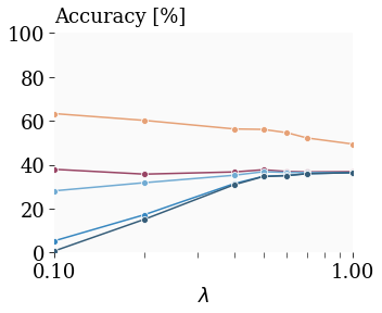
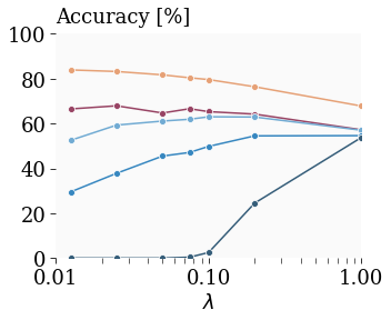
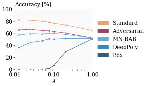
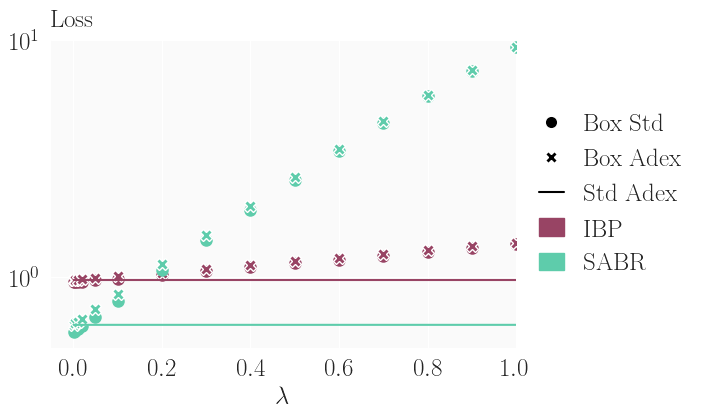
To analyze the interaction between the precision of the certification method and the size of the propagation region, we train a range of models with subselection ratios varying from to and analyze them with verification methods of increasing precision (Box, DeepPoly, MN-BaB). Further, we compute adversarial accuracies using a 50-step PGD attack (Madry et al., 2018) with 5 random restarts and the targeted logit margin loss (Carlini & Wagner, 2017). We illustrate results in Fig. 7 and observe that standard and adversarial accuracies increase with decreasing , as regularization decreases. For , i.e., IBP training, we observe little difference between the verification methods. However, as we decrease , the Box verified accuracy decreases quickly, despite Box relaxations being used during training. In contrast, using the most precise method, MN-BaB, we initially observe increasing certified accuracies, as the reduced regularization yields more accurate networks, before the level of regularization becomes insufficient for certification. While DeepPoly loses precision less quickly than Box, it can not benefit from more accurate networks. This indicates that the increased accuracy, enabled by the reduced regularization, may rely on complex neuron interactions, only captured by MN-BaB. These trends hold across perturbation magnitudes (Figs. 7(b) and 7(a)) and become even more pronounced for narrower networks (Fig. 7(c)), which are more easily over-regularized.
This qualitatively different behavior depending on the precision of the certification method highlights the importance of recent advances in neural network verification for certified training. Even more importantly, these results clearly show that provably robust networks do not necessarily require the level of regularization introduced by IBP training.
Loss Analysis
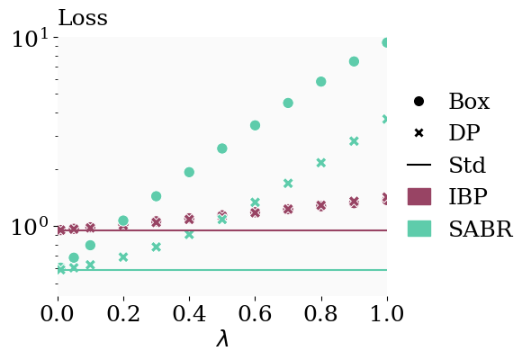
In Fig. 8, we compare the robust loss of a SABR and an IBP trained network across different propagation region sizes (all centred around the original sample) depending on the bound propagation method used. We first observe that, when propagating the full input region (), the SABR trained network yields a much higher robust loss than the IBP trained one. However, when comparing the respective training subselection ratios, for SABR and for IBP, SABR yields significantly smaller training losses. Even more importantly, the difference between robust and standard loss is significantly lower, which, recalling Section 4, directly corresponds to a reduced regularization for robustness and allows the SABR trained network to reach a much lower standard loss. Finally, we observe the losses to clearly grow super-linearly with increasing propagation region sizes (note the logarithmic scaling of the y-axis) when using the Box relaxation, agreeing well with our theoretical results in Section 4. While the more precise DeepPoly (DP) bounds yield significantly reduced robust losses for the SABR trained network, the IBP trained network does not benefit at all, again highlighting its over-regularization. See App. C for extended results.
| Loss | IBP | SABR |
| Std. | ||
| Adv. |
Gradient Alignment
To analyze whether SABR training is actually more aligned with standard accuracy and empirical robustness, as indicated by our theory in Section 4, we conduct the following experiment for CIFAR-10 and : We train one network using SABR with and one with IBP, corresponding to . For both, we now compute the gradients of their respective robust training losses and the cross-entropy loss applied to unperturbed (Std.) and adversarial (Adv.) samples. We then report the mean cosine similarity between these gradients across the whole test set in Table 3. We clearly observe that the SABR loss is much better aligned with both the cross-entropy loss of unperturbed and adversarial samples, corresponding to standard accuracy and empirical robustness, respectively.
| Point | Whole Region | ||||
| Method | Act | Inact | Unst | Act | Inact |
| IBP | 26.2 | 73.8 | 1.18 | 25.6 | 73.2 |
| SABR | 35.9 | 64.1 | 3.67 | 34.3 | 62.0 |
| PGD | 36.5 | 63.5 | 65.5 | 15.2 | 19.3 |
ReLU Activation States
The portion of ReLU activations which are (stably) active, inactive, or unstable has been identified as an important characteristic of certifiably trained networks (Shi et al., 2021). We evaluate these metrics for IBP, SABR, and adversarially (PGD) trained networks on CIFAR-10 at , using the Box relaxation to compute intermediate bounds, and report the average over all layers and test set samples in Table 4. We observe that, when evaluated on concrete points, the SABR trained network has around 37% more active ReLUs than the IBP trained one and almost as many as the PGD trained one, indicating a significantly smaller level of regularization. While the SABR trained network has around -times as many unstable ReLUs as the IBP trained network, when evaluated on the whole input region, it has -times fewer than the PGD trained one, highlighting the improved certifiability.
6 Related Work
Verification Methods
Deterministic verification methods analyse a given network by using abstract interpretation (Gehr et al., 2018; Singh et al., 2018; 2019a), or translating the verification into an optimization problem which they then solve using linear programming (LP) (Palma et al., 2021; Müller et al., 2022; Wang et al., 2021; Zhang et al., 2022c), mixed integer linear programming (MILP) (Tjeng et al., 2019; Singh et al., 2019b), or semidefinite programming (SDP) (Raghunathan et al., 2018; Dathathri et al., 2020). However, as neural network verification is generally NP-complete (Katz et al., 2017), many of these methods trade precision for scalability, yielding so-called incomplete certification methods, which might fail to prove robustness even when it holds. In this work, we analyze our SABR trained networks with deterministic methods.
Certified Training
DiffAI (Mirman et al., 2018) and IBP (Gowal et al., 2018b) minimize a sound over-approximation of the worst-case loss computed using the Box relaxation. Wong et al. (2018) instead use the DeepZ relaxation (Singh et al., 2018), approximated using Cauchy random matrices. Wong & Kolter (2018) compute worst-case losses by back-substituting linear bounds using fixed relaxations. CROWN-IBP (Zhang et al., 2020) uses a similar back-substitution approach but leverages minimal area relaxations introduced by Zhang et al. (2018) and Singh et al. (2019a) to bound the worst-case loss while computing intermediate bounds using the less precise but much faster Box relaxation. Shi et al. (2021) show that they can obtain the same accuracies with much shorter training schedules by combining IBP training with a special initialization. COLT (Balunovic & Vechev, 2020) combines propagation using the DeepZ relaxation with adversarial search. IBP-R (Palma et al., 2022) combines adversarial training with much larger perturbation radii and a ReLU-stability regularization based on the Box relaxation. We compare favorably to all (recent) methods above in our experimental evaluation (see Section 5). Müller et al. (2021) combine certifiable and accurate networks to allow for more efficient trade-offs between robustness and accuracy.
The idea of propagating subsets of the adversarial input region has been explored in the settings of adversarial patches (Chiang et al., 2020) and geometric perturbations (Balunovic et al., 2019), where the number of subsets required to cover the whole region is linear or constant in the input dimensionality. However, these methods are not applicable to the -perturbation setting, we consider, where this scaling is exponential.
Robustness by Construction
Li et al. (2019), Lécuyer et al. (2019), and Cohen et al. (2019) construct locally Lipschitz classifiers by introducing randomness into the inference process, allowing them to derive probabilistic robustness guarantees. Extended in a variety of ways (Salman et al., 2019; Yang et al., 2020), these methods can obtain strong robustness guarantees with high probability (Salman et al., 2019) at the cost of significantly (100x) increased runtime during inference. We focus our comparison on deterministic methods. Zhang et al. (2021) propose a novel architecture, which inherently exhibits -Lipschitzness properties, allowing them to efficiently derive corresponding robustness guarantees. Zhang et al. (2022a) build on this work by improving the challenging training process. Finally, Zhang et al. (2022b) generalize this concept in SortNet.
7 Conclusion
We introduced a novel certified training method called SABR (Small Adversarial Bounding Regions) based on the key insight, that propagating small but carefully selected subsets of the input region combines small approximation errors and thus regularization with well-behaved optimization problems. This allows SABR trained networks to outperform all existing certified training methods on all commonly used benchmarks in terms of both standard and certified accuracy. Even more importantly, SABR lays the foundation for a new class of certified training methods promising to alleviate the robustness-accuracy trade-off and enable the training of networks that are both accurate and certifiably robust.
8 Ethics Statement
As SABR improves both certified and standard accuracy compared to existing approaches, it could help make real-world AI systems more robust to both malicious and random interference. Thus any positive and negative societal effects these systems have could be amplified. Further, while we achieve state-of-the-art results on all considered benchmark problems, this does not (necessarily) indicate sufficient robustness for safety-critical real-world applications, but could give practitioners a false sense of security when using SABR trained models.
9 Reproducibility Statement
We publish our code, all trained models, and detailed instructions on how to reproduce our results at https://github.com/eth-sri/sabr, providing an anonymized version to the reviewers. Further, we provide proofs for our theoretical contributions in App. A and a detailed description of all hyper-parameter choices as well as a discussion of the used data sets including all preprocessing steps in App. C.
Acknowledgements
This work is supported in part by ELSA — European Lighthouse on Secure and Safe AI funded by the European Union under grant agreement No. 101070617. Views and opinions expressed are however those of the authors only and do not necessarily reflect those of the European Union or European Commission. Neither the European Union nor the European Commission can be held responsible for them.
This work has received funding from the Swiss State Secretariat for Education, Research and Innovation (SERI) (SERI-funded ERC Consolidator Grant).
References
- Anil et al. (2019) Cem Anil, James Lucas, and Roger B. Grosse. Sorting out lipschitz function approximation. In Proc. of International Conference on Machine Learning (ICML), volume 97, 2019.
- Balunovic & Vechev (2020) Mislav Balunovic and Martin T. Vechev. Adversarial training and provable defenses: Bridging the gap. In Proc. of ICLR, 2020.
- Balunovic et al. (2019) Mislav Balunovic, Maximilian Baader, Gagandeep Singh, Timon Gehr, and Martin T. Vechev. Certifying geometric robustness of neural networks. In Advances in Neural Information Processing Systems 32: Annual Conference on Neural Information Processing Systems 2019, NeurIPS 2019, December 8-14, 2019, Vancouver, BC, Canada, 2019.
- Biggio et al. (2013) Battista Biggio, Igino Corona, Davide Maiorca, Blaine Nelson, Nedim Srndic, Pavel Laskov, Giorgio Giacinto, and Fabio Roli. Evasion attacks against machine learning at test time. In Machine Learning and Knowledge Discovery in Databases - European Conference, ECML PKDD 2013, Prague, Czech Republic, September 23-27, 2013, Proceedings, Part III, volume 8190, 2013. doi: 10.1007/978-3-642-40994-3\_25.
- Bunel et al. (2020) Rudy Bunel, Jingyue Lu, Ilker Turkaslan, Philip H. S. Torr, Pushmeet Kohli, and M. Pawan Kumar. Branch and bound for piecewise linear neural network verification. J. Mach. Learn. Res., 21, 2020.
- Carlini & Wagner (2017) Nicholas Carlini and David A. Wagner. Towards evaluating the robustness of neural networks. In 2017 IEEE Symposium on Security and Privacy, SP 2017, San Jose, CA, USA, May 22-26, 2017, 2017. doi: 10.1109/SP.2017.49.
- Chiang et al. (2020) Ping-Yeh Chiang, Renkun Ni, Ahmed Abdelkader, Chen Zhu, Christoph Studer, and Tom Goldstein. Certified defenses for adversarial patches. In Proc. of ICLR, 2020.
- Cohen et al. (2019) Jeremy M. Cohen, Elan Rosenfeld, and J. Zico Kolter. Certified adversarial robustness via randomized smoothing. In Proc. of ICML, volume 97, 2019.
- Croce & Hein (2020) Francesco Croce and Matthias Hein. Reliable evaluation of adversarial robustness with an ensemble of diverse parameter-free attacks. In Proc. of ICML, volume 119, 2020.
- Dathathri et al. (2020) Sumanth Dathathri, Krishnamurthy Dvijotham, Alexey Kurakin, Aditi Raghunathan, Jonathan Uesato, Rudy Bunel, Shreya Shankar, Jacob Steinhardt, Ian J. Goodfellow, Percy Liang, and Pushmeet Kohli. Enabling certification of verification-agnostic networks via memory-efficient semidefinite programming. In Advances in Neural Information Processing Systems 33: Annual Conference on Neural Information Processing Systems 2020, NeurIPS 2020, December 6-12, 2020, virtual, 2020.
- Ferrari et al. (2022) Claudio Ferrari, Mark Niklas Müller, Nikola Jovanovic, and Martin T. Vechev. Complete verification via multi-neuron relaxation guided branch-and-bound. In Proc. of ICLR, 2022.
- Gehr et al. (2018) Timon Gehr, Matthew Mirman, Dana Drachsler-Cohen, Petar Tsankov, Swarat Chaudhuri, and Martin T. Vechev. AI2: safety and robustness certification of neural networks with abstract interpretation. In 2018 IEEE Symposium on Security and Privacy, SP 2018, Proceedings, 21-23 May 2018, San Francisco, California, USA, 2018. doi: 10.1109/SP.2018.00058.
- Goodfellow et al. (2015) Ian J. Goodfellow, Jonathon Shlens, and Christian Szegedy. Explaining and harnessing adversarial examples. In Proc. of ICLR, 2015.
- Gowal et al. (2018a) Sven Gowal, Krishnamurthy Dvijotham, Robert Stanforth, Rudy Bunel, Chongli Qin, Jonathan Uesato, Relja Arandjelovic, Timothy A. Mann, and Pushmeet Kohli. On the effectiveness of interval bound propagation for training verifiably robust models. ArXiv preprint, abs/1810.12715, 2018a.
- Gowal et al. (2018b) Sven Gowal, Krishnamurthy Dvijotham, Robert Stanforth, Rudy Bunel, Chongli Qin, Jonathan Uesato, Relja Arandjelovic, Timothy A. Mann, and Pushmeet Kohli. On the effectiveness of interval bound propagation for training verifiably robust models. ArXiv preprint, abs/1810.12715, 2018b.
- Ilyas et al. (2019) Andrew Ilyas, Shibani Santurkar, Dimitris Tsipras, Logan Engstrom, Brandon Tran, and Aleksander Madry. Adversarial examples are not bugs, they are features. In Advances in Neural Information Processing Systems 32: Annual Conference on Neural Information Processing Systems 2019, NeurIPS 2019, December 8-14, 2019, Vancouver, BC, Canada, 2019.
- Ioffe & Szegedy (2015) Sergey Ioffe and Christian Szegedy. Batch normalization: Accelerating deep network training by reducing internal covariate shift. In Proc. of ICML, volume 37, 2015.
- Jovanovic et al. (2021) Nikola Jovanovic, Mislav Balunovic, Maximilian Baader, and Martin T. Vechev. Certified defenses: Why tighter relaxations may hurt training? ArXiv preprint, abs/2102.06700, 2021.
- Katz et al. (2017) Guy Katz, Clark W. Barrett, David L. Dill, Kyle Julian, and Mykel J. Kochenderfer. Reluplex: An efficient SMT solver for verifying deep neural networks. ArXiv preprint, abs/1702.01135, 2017.
- Kingma & Ba (2015) Diederik P. Kingma and Jimmy Ba. Adam: A method for stochastic optimization. In Proc. of ICLR, 2015.
- Krizhevsky et al. (2009) Alex Krizhevsky, Geoffrey Hinton, et al. Learning multiple layers of features from tiny images. 2009.
- Le & Yang (2015) Ya Le and Xuan S. Yang. Tiny imagenet visual recognition challenge. CS 231N, 7(7), 2015.
- LeCun et al. (2010) Yann LeCun, Corinna Cortes, and CJ Burges. Mnist handwritten digit database. ATT Labs [Online]. Available: http://yann.lecun.com/exdb/mnist, 2, 2010.
- Lécuyer et al. (2019) Mathias Lécuyer, Vaggelis Atlidakis, Roxana Geambasu, Daniel Hsu, and Suman Jana. Certified robustness to adversarial examples with differential privacy. In 2019 IEEE Symposium on Security and Privacy, SP 2019, San Francisco, CA, USA, May 19-23, 2019, 2019. doi: 10.1109/SP.2019.00044.
- Li et al. (2019) Bai Li, Changyou Chen, Wenlin Wang, and Lawrence Carin. Certified adversarial robustness with additive noise. In Advances in Neural Information Processing Systems 32: Annual Conference on Neural Information Processing Systems 2019, NeurIPS 2019, December 8-14, 2019, Vancouver, BC, Canada, 2019.
- Madry et al. (2018) Aleksander Madry, Aleksandar Makelov, Ludwig Schmidt, Dimitris Tsipras, and Adrian Vladu. Towards deep learning models resistant to adversarial attacks. In Proc. of ICLR, 2018.
- Mirman et al. (2018) Matthew Mirman, Timon Gehr, and Martin T. Vechev. Differentiable abstract interpretation for provably robust neural networks. In Proc. of ICML, volume 80, 2018.
- Müller et al. (2021) Mark Niklas Müller, Mislav Balunovic, and Martin T. Vechev. Certify or predict: Boosting certified robustness with compositional architectures. In 9th International Conference on Learning Representations, ICLR 2021, Virtual Event, Austria, May 3-7, 2021. OpenReview.net, 2021. URL https://openreview.net/forum?id=USCNapootw.
- Müller et al. (2022) Mark Niklas Müller, Gleb Makarchuk, Gagandeep Singh, Markus Püschel, and Martin T. Vechev. PRIMA: general and precise neural network certification via scalable convex hull approximations. Proc. ACM Program. Lang., 6(POPL), 2022. doi: 10.1145/3498704.
- Palma et al. (2021) Alessandro De Palma, Harkirat S. Behl, Rudy R. Bunel, Philip H. S. Torr, and M. Pawan Kumar. Scaling the convex barrier with active sets. In Proc. of ICLR, 2021.
- Palma et al. (2022) Alessandro De Palma, Rudy Bunel, Krishnamurthy Dvijotham, M. Pawan Kumar, and Robert Stanforth. IBP regularization for verified adversarial robustness via branch-and-bound. ArXiv preprint, abs/2206.14772, 2022.
- Paszke et al. (2019) Adam Paszke, Sam Gross, Francisco Massa, Adam Lerer, James Bradbury, Gregory Chanan, Trevor Killeen, Zeming Lin, Natalia Gimelshein, Luca Antiga, Alban Desmaison, Andreas Köpf, Edward Yang, Zachary DeVito, Martin Raison, Alykhan Tejani, Sasank Chilamkurthy, Benoit Steiner, Lu Fang, Junjie Bai, and Soumith Chintala. Pytorch: An imperative style, high-performance deep learning library. In Advances in Neural Information Processing Systems 32: Annual Conference on Neural Information Processing Systems 2019, NeurIPS 2019, December 8-14, 2019, Vancouver, BC, Canada, 2019.
- Raghunathan et al. (2018) Aditi Raghunathan, Jacob Steinhardt, and Percy Liang. Semidefinite relaxations for certifying robustness to adversarial examples. In Advances in Neural Information Processing Systems 31: Annual Conference on Neural Information Processing Systems 2018, NeurIPS 2018, December 3-8, 2018, Montréal, Canada, 2018.
- Salman et al. (2019) Hadi Salman, Jerry Li, Ilya P. Razenshteyn, Pengchuan Zhang, Huan Zhang, Sébastien Bubeck, and Greg Yang. Provably robust deep learning via adversarially trained smoothed classifiers. In Advances in Neural Information Processing Systems 32: Annual Conference on Neural Information Processing Systems 2019, NeurIPS 2019, December 8-14, 2019, Vancouver, BC, Canada, 2019.
- Shi et al. (2021) Zhouxing Shi, Yihan Wang, Huan Zhang, Jinfeng Yi, and Cho-Jui Hsieh. Fast certified robust training via better initialization and shorter warmup. ArXiv preprint, abs/2103.17268, 2021.
- Singh et al. (2018) Gagandeep Singh, Timon Gehr, Matthew Mirman, Markus Püschel, and Martin T. Vechev. Fast and effective robustness certification. In Advances in Neural Information Processing Systems 31: Annual Conference on Neural Information Processing Systems 2018, NeurIPS 2018, December 3-8, 2018, Montréal, Canada, 2018.
- Singh et al. (2019a) Gagandeep Singh, Timon Gehr, Markus Püschel, and Martin T. Vechev. An abstract domain for certifying neural networks. Proc. ACM Program. Lang., 3(POPL), 2019a. doi: 10.1145/3290354.
- Singh et al. (2019b) Gagandeep Singh, Timon Gehr, Markus Püschel, and Martin T. Vechev. Boosting robustness certification of neural networks. In Proc. of ICLR, 2019b.
- Szegedy et al. (2014) Christian Szegedy, Wojciech Zaremba, Ilya Sutskever, Joan Bruna, Dumitru Erhan, Ian J. Goodfellow, and Rob Fergus. Intriguing properties of neural networks. In Proc. of ICLR, 2014.
- Tjeng et al. (2019) Vincent Tjeng, Kai Y. Xiao, and Russ Tedrake. Evaluating robustness of neural networks with mixed integer programming. In Proc. of ICLR, 2019.
- Tramèr et al. (2020) Florian Tramèr, Nicholas Carlini, Wieland Brendel, and Aleksander Madry. On adaptive attacks to adversarial example defenses. In Advances in Neural Information Processing Systems 33: Annual Conference on Neural Information Processing Systems 2020, NeurIPS 2020, December 6-12, 2020, virtual, 2020.
- Wang et al. (2021) Shiqi Wang, Huan Zhang, Kaidi Xu, Xue Lin, Suman Jana, Cho-Jui Hsieh, and J. Zico Kolter. Beta-crown: Efficient bound propagation with per-neuron split constraints for neural network robustness verification. In Advances in Neural Information Processing Systems 34: Annual Conference on Neural Information Processing Systems 2021, NeurIPS 2021, December 6-14, 2021, virtual, 2021.
- Wong & Kolter (2018) Eric Wong and J. Zico Kolter. Provable defenses against adversarial examples via the convex outer adversarial polytope. In Proc. of ICML, volume 80, 2018.
- Wong et al. (2018) Eric Wong, Frank R. Schmidt, Jan Hendrik Metzen, and J. Zico Kolter. Scaling provable adversarial defenses. In Advances in Neural Information Processing Systems 31: Annual Conference on Neural Information Processing Systems 2018, NeurIPS 2018, December 3-8, 2018, Montréal, Canada, 2018.
- Xu et al. (2020) Kaidi Xu, Zhouxing Shi, Huan Zhang, Yihan Wang, Kai-Wei Chang, Minlie Huang, Bhavya Kailkhura, Xue Lin, and Cho-Jui Hsieh. Automatic perturbation analysis for scalable certified robustness and beyond. In Advances in Neural Information Processing Systems 33: Annual Conference on Neural Information Processing Systems 2020, NeurIPS 2020, December 6-12, 2020, virtual, 2020.
- Yang et al. (2020) Greg Yang, Tony Duan, J. Edward Hu, Hadi Salman, Ilya P. Razenshteyn, and Jerry Li. Randomized smoothing of all shapes and sizes. In Proc. of ICML, volume 119, 2020.
- Zhang et al. (2021) Bohang Zhang, Tianle Cai, Zhou Lu, Di He, and Liwei Wang. Towards certifying l-infinity robustness using neural networks with l-inf-dist neurons. In Proc. of ICML, volume 139, 2021.
- Zhang et al. (2022a) Bohang Zhang, Du Jiang, Di He, and Liwei Wang. Boosting the certified robustness of l-infinity distance nets. In Proc. of ICLR, 2022a.
- Zhang et al. (2022b) Bohang Zhang, Du Jiang, Di He, and Liwei Wang. Rethinking lipschitz neural networks and certified robustness: A boolean function perspective. CoRR, abs/2210.01787, 2022b. doi: 10.48550/arXiv.2210.01787. URL https://doi.org/10.48550/arXiv.2210.01787.
- Zhang et al. (2018) Huan Zhang, Tsui-Wei Weng, Pin-Yu Chen, Cho-Jui Hsieh, and Luca Daniel. Efficient neural network robustness certification with general activation functions. In Advances in Neural Information Processing Systems 31: Annual Conference on Neural Information Processing Systems 2018, NeurIPS 2018, December 3-8, 2018, Montréal, Canada, 2018.
- Zhang et al. (2020) Huan Zhang, Hongge Chen, Chaowei Xiao, Sven Gowal, Robert Stanforth, Bo Li, Duane S. Boning, and Cho-Jui Hsieh. Towards stable and efficient training of verifiably robust neural networks. In Proc. of ICLR, 2020.
- Zhang et al. (2022c) Huan Zhang, Shiqi Wang, Kaidi Xu, Linyi Li, Bo Li, Suman Jana, Cho-Jui Hsieh, and J. Zico Kolter. General cutting planes for bound-propagation-based neural network verification. ArXiv preprint, abs/2208.05740, 2022c.
Appendix A Deferred Proofs
In this section, we provide the proof for Lemma A.1. Let us first consider the following Lemma:
Lemma A.1 (Hyper-Box Growth).
Let be a ReLU function and consider box inputs with radius and centres . Then the mean radius of the output boxes will satisfy:
| (9) |
and
| (10) |
Proof.
Recall that given an input box with centre and radius , the output relaxation of a ReLU layer is defined by:
| (11) |
We thus obtain the expectation
| (12) |
its derivative
| (13) |
and its curvature
| (14) |
∎
Now, we can easily proof Theorem 4.1, restated below for convenience.
See 4.1
Proof.
Example for Piecewise Uniform Distribution
Let us assume the centres are distributed according to:
| (15) |
where and . Then we have by Lemma A.1
| (16) | ||||
| (17) | ||||
| (18) |
We observe quadratic growth for and recover the symmetric special case of for .
Appendix B Additional Theoretical Details
B.1 Cross-Entropy Loss Formulation
Below we derive the formulation of the Cross-Entropy (CE) loss used in equation Eqs. 2 and 5. We let be the label probability of class , the predicted probability of class , the label for sample and the logits predicted by a neural network for this sample.
Appendix C Additional Experimental Details
In this section, we provide detailed informations on the exact experimental setup.
Datasets
We conduct experiments on the MNIST (LeCun et al., 2010), CIFAR-10 (Krizhevsky et al., 2009), and TinyImageNet (Le & Yang, 2015) datasets. For TinyImageNet and CIFAR-10 we follow Shi et al. (2021) and use random horizontal flips and random cropping as data augmentation during training and normalize inputs after applying perturbations. Following prior work (Xu et al., 2020; Shi et al., 2021), we evaluate CIFAR-10 and MNIST on their test sets and TinyImageNet on its validation set, as test set labels are unavailable. Following Xu et al. (2020) and in contrast to Shi et al. (2021), we train and evaluate TinyImageNet with images cropped to .
| Dataset | |||
| MNIST | 0.1 | 0.4 | |
| 0.3 | 0.6 | ||
| CIFAR-10 | 2/255 | 0.1 | |
| 8/255 | 0 | 0.7 | |
| TinyImageNet | 1/255 | 0.4 |
Training Hyperparameters
We mostly follow the hyperparameter choices from Shi et al. (2021) including their weight initialization and warm-up regularization222For the ReLU warm-up regularization, the bounds of the small boxes are considered., and use ADAM (Kingma & Ba, 2015) with an initial learning rate of , decayed twice with a factor of 0.2. For CIFAR-10 we train an epochs for and , respectively, decaying the learning rate after and and and epochs. For TinyImageNet we use the same settings as for CIFAR-10 at . For MNIST we train epochs, decaying the learning rate after and epochs. We choose a batch size of for CIFAR-10 and TinyImageNet, and for MNIST. We use regularization with factors according to Table 5. For all datasets, we perform one epoch of standard training () before annealing from to its final value over epochs for CIFAR-10 and TinyImageNet and for epochs for MNIST. We use an step PGD attack with an initial step size of , decayed with a factor of after the th and th step to select the centre of the propagation region. We use a constant subselection ratio with values shown in Table 5. For CIFAR-10 we use shrinking with (see below).
ReLU-Transformer with Shrinking
Additionally to standard SABR, outlined in Section 3, we propose to amplify the Box growth rate reduction (see Section 4) affected by smaller propagation regions, by adapting the ReLU transformer as follows:
| (19) |
We call the shrinking coefficient, as the output radius of unstable ReLUs is shrunken by multiplying it with this factor. We note that we only use these transformers for the CIFAR-10 network discussed in Table 1.
Architectures
Similar to prior work (Shi et al., 2021), we consider a 7-layer convolutional architecture, CNN7. The first 5 layers are convolutional layers with filter sizes [64, 64, 128, 128, 128], kernel size 3, strides [1, 1, 2, 1, 1], and padding 1. They are followed by a fully connected layer with 512 hidden units and the final classification. All but the last layers are followed by batch normalization (Ioffe & Szegedy, 2015) and ReLU activations. For the BN layers, we train using the statistics of the unperturbed data similar to Shi et al. (2021). During the PGD attack we use the BN layers in evaluation mode. We further consider narrower version, CNN7-narrow which is identical to CNN7 expect for using the filter sizes [32, 32, 64, 64, 64] and a fully connected layer with 216 hidden units.
| Dataset | Time | |
| MNIST | 0.1 | 3h 23 min |
| 0.3 | 3h 20 min | |
| CIFAR-10 | 2/255 | 7h 6 min |
| 8/255 | 7h 20 min | |
| TinyImageNet | 1/255 | 57h 24 min |
Hardware and Timings
We train and certify all networks using single NVIDIA RTX 2080Ti, 3090, Titan RTX, or A6000. Training takes roughly and hours for MNIST and CIFAR-10, respectively, with TinyImageNet taking two and a half days on a single NVIDIA RTX 2080Ti. For more Details see Table 6. Verification with MN-BaB takes around h for MNIST, h for CIFAR-10 and h for TinyImageNet on a NVIDIA Titan RTX.
Appendix D Additional Experimental Results
Loss Analysis
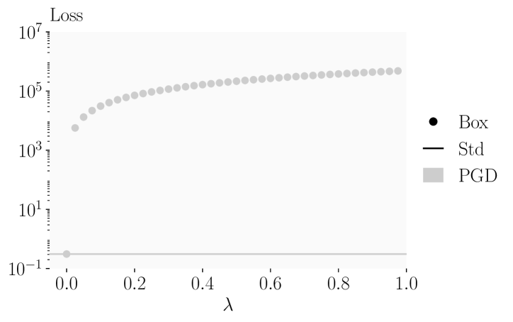
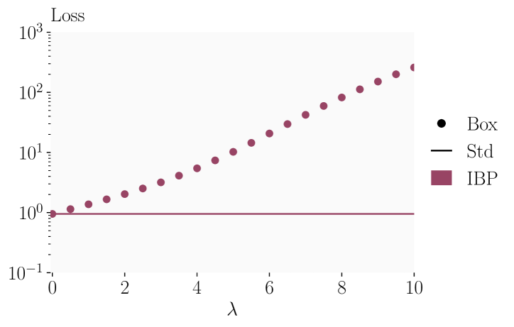
In Fig. 9, we show the error growth of an adversarially trained (left) and IBP trained model over increasing subselection ratios . We observe that errors grow only slightly super-linear rather than exponential for the adversarially trained network. We trace this back to the large portion of crossing ReLUs (Table 4), especially in later layers, leading to the layer-wise growth being only linear. For the IBP trained model, in contrast, we observe exponential growth across a wide range of propagation region sizes, as the heavy regularization leads to a small portion of active and unstable ReLUs. In Fig. 10, we compare errors for Box centred around the unperturbed sample (Box Std) and around a high loss point computed with an adversarial attack (Box Adex). We observe that while the loss is larger around the adversarial centres, especially for small propagation regions, this effect is small compared to the difference between training or certification methods.
Training Method Source Acc. [%] Adv. Acc. [%] Cert. Acc. [%] 2/255 COLT Balunovic & Vechev (2020) 78.42 66.17 61.02 CROWN-IBP Zhang et al. (2020)† 71.27 59.58 58.19 IBP Shi et al. (2021) - - - SABR this work 79.52 65.76 62.57 8/255 COLT Balunovic & Vechev (2020) 51.69 31.81 27.60 CROWN-IBP Zhang et al. (2020)† 45.41 33.33 33.18 IBP Shi et al. (2021) 48.94 35.43 35.30 SABR this work 52.00 35.70 35.25 - No network published. Published network does not match reported performance.
D.1 Effect of Verification Method on Other Certified Defenses
In this section we compare different certified defenses when evaluated using the same, precise verifier MN-BaB (Ferrari et al., 2022). While COLT (Balunovic & Vechev, 2020) and IBP-R (Palma et al., 2022) trained networks were verified using similarly expensive and precise verification methods as MN-BaB (MILP (Tjeng et al., 2019) and -CROWN (Wang et al., 2021), respectively), the IBP and CROWN-IBP trained networks were originally verified using much less precise Box propagation. We compare standard (Acc.), empirical adversarial (Adv. Acc.), and certified (Cert. Acc.) accuracy for CIFAR-10 at and in Table 7. We omit IBP-R, as neither code nor networks are published. For CROWN-IBP (Zhang et al., 2020), we evaluated both the ‘best’ and last checkpoints of the published networks but observed that the standard accuracy of neither matched the ones reported in the paper. We report the better of the two (‘best’).
We observe that certified accuracies increase only minimal in most settings, with the exception of CROWN-IBP at , where the certified accuracy rises from to . However, there the adversarial accuracy of remains significantly below our certified accuracy of . At the IBP trained network achieves certified accuracy, matching SABR’s performance, however at a lower standard accuracy.
| Training Method | Acc. [%] | Cert. Acc. [%] |
| SABR | 80.4 | 61.0 |
| centred | 82.5 | 27.4 |
| random | 84.1 | 28.3 |
| FGSM | 80.8 | 58.2 |
| no projection | 80.0 | 61.9 |
| CROWN-IBP | 80.3 | 56.7 |
D.2 Ablation SABR
To assess the different components of SABR, we conduct an ablation study on CIFAR-10 with . Beyond the subselection ratio /, discussed in Section 5 and especially Fig. 7, SABR has two main components: i) the choice of propagation region position and ii) the propagation method.
To analyse the effect of the propagation region’s position, we evaluate four methods to compute its center for : i) always choose the original input as center (centred: ), ii) choose the center uniformly at random such that the propagation region lies in the original adversarial region (random: ), iii) choose the centre with a weak adversarial attack such as FGSM (Goodfellow et al., 2015) (FGSM: ), and iv) choose the centre with a strong adversarial attack over the whole input region , without projecting it into , allowing it to ‘stick out’ (no projection: ). We observe that choosing centres either at random or as the original input leads to weaker regularization, increasing standard accuracy slightly ( and , respectively) but significantly reducing certified accuracy ( and , respectively). Using a weaker adversarial attack has a similar but much less pronounced effect, increasing natural accuracy by at the cost of a reduction in certified accuracy. Permitting propagation regions to protrude from the original input region increases regularization, leading to a slight increase in certified accuracy () at the cost of decreased standard accuracy ().
To assess the effect of the propagation method, we compare standard SABR which uses IBP, yielding an easier optimization problem (Jovanovic et al., 2021), to CROWN-IBP, which generally yields tighter bounds. We observe that using the less precise Box propagation indeed yields better standard and certified accuracy.
D.3 Bound Tightness
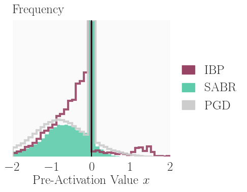
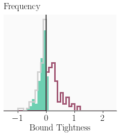
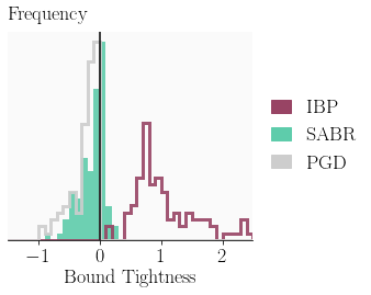
To support the intuitions discussed in Section 3, we compare the tightness of IBP, SABR, and PGD bounds on the worst-case margin loss. To make the computation of the exact worst-case loss () via mixed integer linear programming (MILP) and using the encoding from Tjeng et al. (2019) tractable, we train a small network (2 convolutional layers and 1 linear layer) with IBP and SABR () on MNIST at . We compute bounds on the minimum logit difference for the first 100 test set samples using SABR as during training (-step PGD attack targeting the Cross-Entropy loss), using PGD with a -step margin attack and restarts per adversarial label, and using IBP.
In Fig. 11, we show histograms of the bound tightness (), where results greater 0 correspond to the bound (PGD, IBP, or SABR) being larger than the actual worst case loss and results smaller 0 correspond to the bound being smaller. A sound verification method will thus always yield positive bound tightness and is the more precise the smaller its absolute value. Similarly, adversarial attack based methods will always yield negative bounds, with stronger attacks generally yielding smaller magnitudes.
We observe that, especially for the SABR trained network, IBP bounds are relatively loose. SABR bounds are generally tighter than both PGD and IBP bounds (smaller mean magnitude), although clearly not sound (as discussed in Section 3). We highlight that the PGD attack used to compute the bound is significantly stronger than the one used for SABR. We conclude that while SABR bounds often do not include the true worst case loss, they represent a better proxy than either IBP or PGD bounds.
| Layer | PGD | SABR | IBP | |||
| mean | max | mean | max | mean | max | |
| Conv 1∗ | ||||||
| Conv 2∗ | ||||||
| Conv 3∗ | ||||||
| Conv 4∗ | ||||||
| Conv 5∗ | ||||||
| Lin 1∗ | ||||||
| Lin 2 | ||||||
D.4 Box Growth Rates of Trained Networks
In Table 9, we compare the mean and max row-wise -norm of the effective weight matrices of PGD, SABR and IBP trained networks for CIFAR-10 and , depending on the network layer. Where applicable, we combine batch normalization layers with the preceding affine layers. As we show in Section 4, this corresponds to the mean and maximum growth rate for Box of equal side lengths.
We observe that growth rates generally increase with network depth. Interestingly training with Box, either in the form of SABR or IBP significantly reduces growth rates in the early layers, but much less in later layers. For IBP trained networks, the maximum growth rate in later layers can even exceed that of the PGD trained network.