Sequential Neural Score Estimation: Likelihood-Free Inference with Conditional Score Based Diffusion Models

Abstract

We introduce Sequential Neural Posterior Score Estimation (SNPSE) and Sequential Neural Likelihood Score Estimation (SNLSE), two new score-based methods for Bayesian inference in simulator-based models. Our methods, inspired by the success of score-based methods in generative modelling, leverage conditional score-based diffusion models to generate samples from the posterior distribution of interest. These models can be trained using one of two possible objective functions, one of which approximates the score of the intractable likelihood, while the other directly estimates the score of the posterior. We embed these models into a sequential training procedure, which guides simulations using the current approximation of the posterior at the observation of interest, thereby reducing the simulation cost. We validate our methods, as well as their amortised, non-sequential variants, on several numerical examples, demonstrating comparable or superior performance to existing state-of-the-art methods such as Sequential Neural Posterior Estimation (SNPE) and Sequential Neural Likelihood Estimation (SNLE).

(a) True posterior.

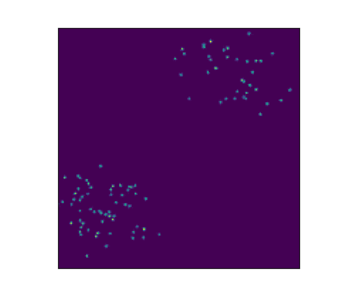
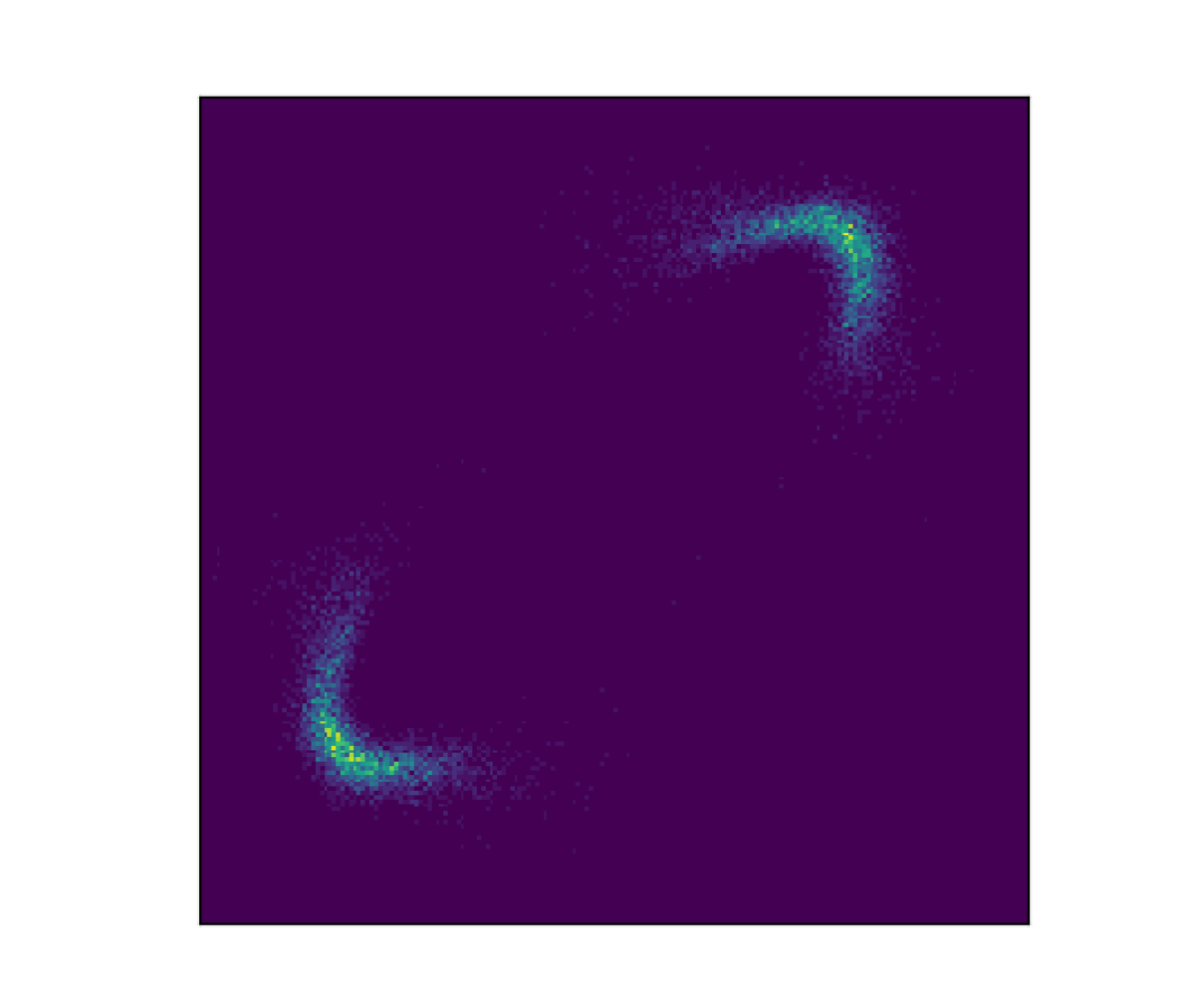
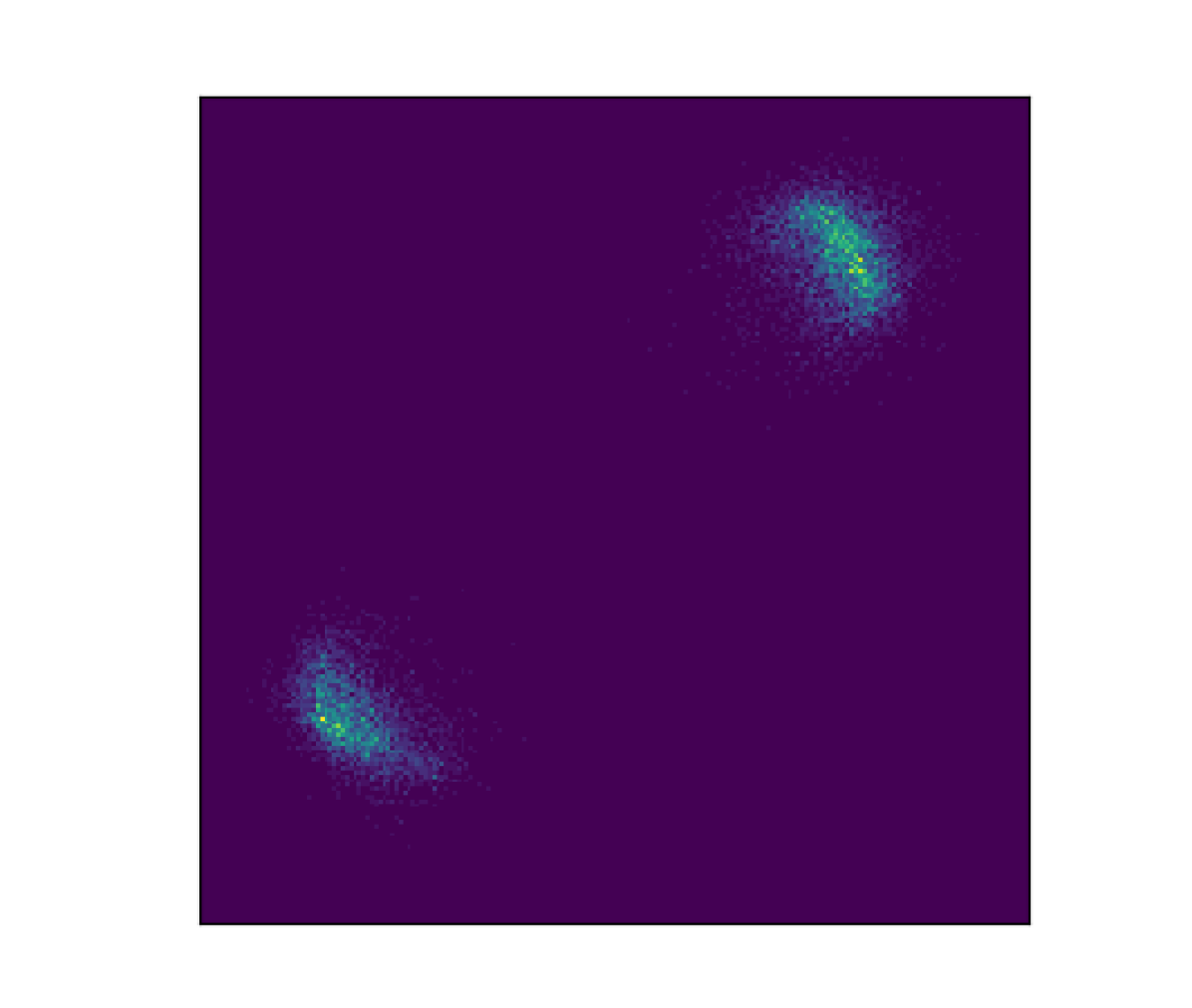
(b) Existing algorithms: SMC-ABC (top left), SNLE (top right), SNPE (bottom left), SNRE (bottom right).

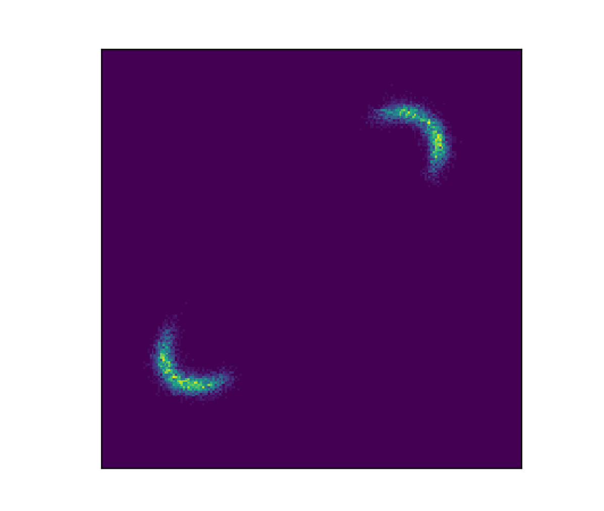
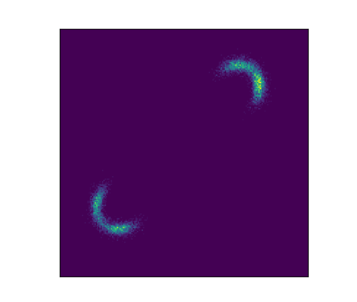
(c) Our algorithms: NLSE (top left), NPSE (top right), SNLSE (bottom left), SNPSE (bottom right).

Figure 1: A comparison between existing SBI algorithms and our algorithms. Plots of the posterior samples for the ‘two moons’ experiment (see Section 5.2). We train each algorithm using $1000$ samples $(\theta,x)\sim p(\theta)p(x|\theta)$.

1 Introduction

Many applications in science, engineering, and economics make use of stochastic numerical simulations to model complex phenomena of interest. Such simulator-based models are typically designed by domain experts, using knowledge of the underlying principles of the process of interest. They are thus particularly well suited to domains in which observations are best understood as the result of mechanistic physical processes. These include, amongst others, neuroscience (Sterratt et al., 2011; Gonçalves et al., 2020), evolutionary biology (Beaumont et al., 2002; Ratmann et al., 2007), ecology (Beaumont, 2010; Wood, 2010), epidemiology (Corander et al., 2017), climate science (Holden et al., 2018), cosmology (Alsing et al., 2018, 2019), high-energy physics (Brehmer et al., 2018; Brehmer, 2021), and econometrics (Gourieroux et al., 1993; Monfardini, 1998).

In many cases, simulator-based models depend on parameters $\theta$ which cannot be identified experimentally, and must be inferred from data $x$. Bayesian inference provides a principled approach for this task. In particular, given a prior $p(\theta)$ and a likelihood $p(x|\theta)$, Bayes’ Theorem gives the posterior distribution over the parameters as

$$p(\theta|x)=\frac{p(x|\theta)p(\theta)}{p(x)}$$ (1)

where $p(x)=\int_{\mathbb{R}^{n}}p(x|\theta)p(\theta)\mathrm{d}\theta$ is known as the evidence, or the marginal likelihood.

The major difficulty associated with simulator-based models is the absence of a tractable likelihood function $p(x|\theta)$. This precludes, in particular, the direct use of conventional likelihood-based Bayesian inference methods, such as Markov chain Monte Carlo (MCMC) (Brooks et al., 2011) and variational inference (VI) (Blei et al., 2017). The resulting inference problem is often referred to as likelihood-free inference (LFI) or simulation-based inference (SBI) (Cranmer et al., 2020; Sisson et al., 2018a).

Traditional methods for performing SBI include approximate Bayesian computation (ABC) (Beaumont et al., 2002; Sisson et al., 2018a), whose variants include rejection ABC (Tavaré et al., 1997; Pritchard et al., 1999), MCMC ABC (Marjoram et al., 2003), and sequential Monte Carlo (SMC) ABC (Beaumont et al., 2009; Bonassi & West, 2015). In such methods, one repeatedly samples parameters, and only accepts parameters for which the samples from the simulator are similar to the observed data $x_{\text{obs}}$. This similarity is typically assessed by computing some measure of distance between summary statistics of the observed data and the simulated data. While ABC has found success in many applications (Sisson et al., 2018b), it has certain notable shortcomings. For example, as the dimensionality increases, this approach suffers from an exponentially increasing simulation cost. It also requires the design of suitable distance functions, summary statistics, and acceptance thresholds.

In recent years, a range of new SBI methods have been introduced, leveraging advances in machine learning such as normalising flows (Papamakarios et al., 2017, 2021) and generative adversarial networks (Goodfellow et al., 2014). These methods often include a sequential training procedure, which adaptively guides simulations to yield more informative data. Such methods include Sequential Neural Posterior Estimation (SNPE) (Papamakarios & Murray, 2016; Lueckmann et al., 2017; Greenberg et al., 2019), Sequential Neural Likelihood Estimation (SNLE) (Lueckmann et al., 2019; Papamakarios et al., 2019), and Sequential Neural Ratio Estimation (SNRE) (Durkan et al., 2020; Hermans et al., 2020; Miller et al., 2021; Thomas et al., 2022). Other more recent algorithms of a similar flavour include Sequential Neural Variational Inference (SNVI) (Glockler et al., 2022), Sequential Neural Posterior and Likelihood Approximation (SNPLA) (Wiqvist et al., 2021), and Generative Adversarial Training for SBI (GATSBI) (Ramesh et al., 2022).

In this paper, we present Neural Likelihood Score Estimation (NLSE) and Neural Posterior Score Estimation (NPSE), as well as their sequential variants SNLSE and SNPSE. Inspired by the remarkable success of score-based generative models (Song & Ermon, 2019; Song et al., 2021b; Ho et al., 2020), our methods train conditional score-based diffusion models to generate samples from the posterior of interest. While similar approaches (e.g., Batzolis et al., 2021; Dhariwal & Nichol, 2021; Song et al., 2021b; Tashiro et al., 2021; Chao et al., 2022; Chung et al., 2022; Geffner et al., 2022) have previously found success in a variety of problems, their application to problems of interest to the SBI community (see, e.g., Lueckmann et al., 2021) has not yet been widely investigated. In parallel with this work, we note that Geffner et al. (2022) have also studied the use of conditional score-based diffusion models for LFI. We provide a more detailed comparison with this paper in Section 4.3 and Appendix D.

In contrast to existing SBI approaches based on normalising flows (e.g., SNLE, SNPE), our approach only requires estimates for the gradient of the log density, or score function, of the intractable likelihood or the posterior, which can be estimated using a neural network via score matching (Hyvärinen, 2005; Vincent, 2011; Song et al., 2020). Since we do not require a normalisable model, we avoid the need for any strong restrictions on the model architecture. In addition, unlike methods based on generative adversarial networks (e.g., GATSBI), we do not require adversarial training objectives, which are notoriously unstable (Metz et al., 2017; Salimans et al., 2016).

We discuss two training objectives for our model; the first targets the score of the intractable likelihood, while the second targets the score of the posterior. We then show how this model can be embedded within a principled sequential training procedure, which guides simulations towards informative regions using the current approximation of the posterior score. We validate the performance of our methods on several benchmark SBI problems, obtaining comparable or superior performance to other state-of-the-art methods.

The remainder of this paper is organised as follows. In Section 2, we introduce score-based diffusion models and outline how these can be used for LFI. In Section 3, we introduce sequential versions of our approaches. In Section 4, we survey some related work. In Section 5, we provide numerical results to validate our approach. Finally, in Section 6, we provide some concluding remarks.

2 Likelihood Free Inference with Score Estimation

2.1 Likelihood Free Inference

Consider a simulator that generates data $x\in\mathbb{R}^{d}$ for any set of parameters $\theta\in\mathbb{R}^{n}$. Suppose that the parameters are distributed according to some known prior $p(\theta)$, but that the likelihood $p(x|\theta)$ is only known implicity via a simulator. Given an observation $x_{\text{obs}}$, we are interested in sampling from the posterior distribution $p(\theta|x_{\text{obs}})\propto p(x_{\text{obs}}|\theta)p(\theta)$, given a finite number of i.i.d. samples $(\theta_{i},x_{i})_{i=1}^{n}\sim p(\theta)p(x|\theta)$.

2.2 Score-Based Likelihood Free Inference

We now outline the key components of score-based likelihood-free inference. Our presentation of the material in this section closely follows the discussion of score-based generative models in (Song & Ermon, 2019), adapted appropriately to conditional setting.

2.2.1 Score Estimation

The first ingredient of score-based LFI is an estimate for the score of the unknown posterior distribution $s_{\psi}(\theta,x)\approx\nabla_{\theta}\log p(\theta|x)$. We outline two natural approaches for obtaining this estimate.

Posterior Score Estimation

The first approach is to directly obtain an estimate for the posterior score $s_{\psi_{\mathrm{post}}}(\theta,x)\approx\nabla_{\theta}\log p(\theta|x)$ by minimising the Fisher divergence between the model and the posterior, viz

$$\frac{1}{2}\mathbb{E}_{p(\theta,x)}\left[||s_{\psi_{\mathrm{post}}}(\theta,x)-\nabla_{\theta}\log p(\theta|x)||^{2}\right].$$ (2)

Clearly, this objective is intractable, since it requires access to the unknown posterior score $\nabla_{\theta}\log p(\theta|x)$. Fortunately, an existing family of methods known as score matching make it possible to minimise the Fisher divergence without needing to evaluate this quantity (Hyvärinen, 2005; Vincent, 2011; Song et al., 2020).

We will focus on the conditional version of a method known as denoising score matching (Vincent, 2011). According to this approach, one first perturbs prior samples $\theta\sim p(\theta)$ according to some pre-determined noise distribution $p_{\sigma}(\tilde{\theta}|\theta)$. One then uses score matching to estimate the score of the perturbed posterior distribution $p_{\sigma}(\tilde{\theta}|x)=\int_{\mathbb{R}^{d}}p_{\sigma}(\tilde{\theta}|\theta)p(\theta|x)\mathrm{d}\theta$.

Crucially, it is possible to show that minimising the posterior score matching objective (2) over the perturbed samples is equivalent to minimising the denoising posterior score matching objective

$$\frac{1}{2}\mathbb{E}_{p_{\sigma}(\tilde{\theta}|\theta)p(\theta,x)}\left[||s_{{\psi_{\mathrm{post}}}}(\tilde{\theta},x)-\nabla_{\tilde{\theta}}\log p_{\sigma}(\tilde{\theta}|\theta)||^{2}\right],$$ (3)

which is simple to compute for any suitable choice of the noise distribution $p_{\sigma}(\tilde{\theta}|\theta)$. In particular, this objective is uniquely minimised when $s_{\psi_{\mathrm{post}}}(\theta,x)=\nabla_{{\theta}}\log p_{\sigma}(\theta|x)$ almost surely. Provided the perturbation is close to zero, we have $\nabla_{\theta}\log p(\theta|x)\approx\nabla_{\theta}\log p_{\sigma}(\theta|x)\approx s_{\psi_{\mathrm{post}}}(\theta,x)$, and thus the score network can be used as an estimate for the true posterior score.

Likelihood Score Estimation

Our second approach is based on the simple observation that

$$\nabla_{\theta}\log p(\theta|x)=\nabla_{\theta}\log p(x|\theta)+\nabla_{\theta}\log p(\theta).$$ (4)

In most cases of interest, $\nabla_{\theta}\log p(\theta)$ is known. Thus, in estimate the posterior score , we simply require an estimate for the score of the intractable likelihood, $s_{\psi_{\mathrm{lik}}}(\theta,x)\approx\nabla_{\theta}\log p(x|\theta)$. Similar to before, we can obtain such an estimate by minimising the Fisher divergence between the model and the likelihood, namely,

$$\frac{1}{2}\mathbb{E}_{p(\theta,x)}\left[||s_{\psi_{\mathrm{lik}}}(\theta,x)-\nabla_{\theta}\log p(x|\theta)||^{2}\right].$$ (5)

This objective remains intractable due to the unknown $\nabla_{\theta}\log p(x|\theta)$. However, as before, we can use ideas from denoising score matching to obtain a tractable objective.

In particular, in this case one can show that the unique minimiser of the likelihood score matching objective (5), computed with respect to the perturbed samples, coincides with the unique minimiser of the so-called denoising likelihood score matching objective (Chao et al., 2022)

$$\frac{1}{2}\mathbb{E}_{p_{\sigma}(\tilde{\theta}|\theta)p(\theta,x)} \left[||s_{\psi_{\mathrm{lik}}}(\tilde{\theta},x)+\nabla_{\tilde{\theta}}\log p_{\sigma}(\tilde{\theta})\right.$$

$$\hskip 45.5244pt-\left.\nabla_{\tilde{\theta}}\log p_{\sigma}(\tilde{\theta}|\theta)||^{2}\right].$$ (6)

Unlike the denoising posterior score matching objective (3), this objective depends on $\smash{\nabla_{\tilde{\theta}}\log p_{\sigma}(\tilde{\theta})}$, the score of the perturbed prior. For certain choices of the prior $p(\theta)$ and the noise distribution $p_{\sigma}(\tilde{\theta}|\theta)$, it is possible to compute $\smash{p_{\sigma}(\tilde{\theta})=\int_{\mathbb{R}^{d}}p(\tilde{\theta}|\theta)p(\theta)\mathrm{d}\theta}$ in closed form. In such cases, one can obtain $\smash{s_{\psi_{\mathrm{pri}}}(\tilde{\theta})=\nabla_{\tilde{\theta}}\log p_{\sigma}(\tilde{\theta})}$ analytically, or by using automatic differentiation (Bücker et al., 2006).

In cases where this is not possible, it is necessary to substitute an estimate $s_{\psi_{\mathrm{pri}}}(\theta)\approx\nabla_{\tilde{\theta}}\log p_{\sigma}(\tilde{\theta})$ in (6). To obtain such an estimate, we can simply train a score network for the prior by minimising the standard denoising score matching objective

$$\frac{1}{2}\mathbb{E}_{p_{\sigma}(\tilde{\theta}|\theta)p(\theta)}\left[||s_{\psi_{\mathrm{pri}}}(\tilde{\theta})-\nabla_{\tilde{\theta}}\log p_{\sigma}(\tilde{\theta}|\theta)||^{2}\right].$$ (7)

Indeed, classical results tell us that this is uniquely minimised when $s_{\psi_{\mathrm{pri}}}(\tilde{\theta})=\nabla_{\tilde{\theta}}\log p_{\sigma}(\tilde{\theta})$ a.s. (Vincent, 2011).

In either case, based on (4), we can now estimate the posterior score as $\smash{s_{\psi_{\mathrm{post}}}(\theta,x)=s_{\psi_{\mathrm{lik}}}(\theta,x)+s_{\psi_{\mathrm{pri}}}(\theta)}$, where $\smash{\psi_{\text{post}}=(\psi_{\text{lik}},\psi_{\text{pri}})^{T}}$.

2.2.2 Sampling

The second key ingredient of a score-based LFI method is a gradient-based sampling algorithm. Possible choices include stochastic gradient Langevin dynamics (SGLD) (Welling & Teh, 2011; Song & Ermon, 2019), Stein variational gradient descent (Liu & Wang, 2016), and Hamiltonian Monte Carlo (Betancourt, 2017). In particular, to generate samples from $p(\theta|x_{\text{obs}})$, one can now simply substitute $s_{\psi_{\mathrm{post}}}(\theta,x_{\text{obs}})\approx\nabla_{\theta}\log p(\theta|x_{\text{obs}})$ into the sampling scheme of choice.

In practice, this naive approach has several fundamental limitations, as first observed by Song & Ermon (2019) in the context of generative modelling. In particular, the scarcity of data in low density regions can cause inaccurate score estimation, and slow mixing (Song & Ermon, 2019). Moreover, the explicit score matching objective is inconsistent when the distribution has compact support (Hyvärinen, 2005).

2.3 Likelihood Free Inference with Conditional Score Based Diffusion Models

These issues are addressed by conditional score-based diffusion models (Song & Ermon, 2019; Ho et al., 2020; Song et al., 2021a, b; Bortoli et al., 2022; Chao et al., 2022). These models can be described as follows. To begin, noise is gradually added to the target distribution using a diffusion process, resulting in a tractable noise distribution from which it is straightforward to sample (e.g., multivariate Gaussian). The time-reversal of this process is also a diffusion process, which depends on the time-dependent scores of the perturbed posterior distributions. These can be estimated using a time-dependent score network, using denoising score matching. Finally, samples from the posterior can be obtained by simulating the approximate reverse-time process, initialised at samples from the noise distribution.

We will now outline this approach in greater detail, focusing in particular on how it can be used for LFI.

2.3.1 The Forward Process

We begin by defining a forward noising process $(\theta_{t})_{t\in[0,T]}$ according to the stochastic differential equation (SDE)

$$\mathrm{d}\theta_{t} =f(\theta_{t},t)\mathrm{d}t+g(t)\mathrm{d}w_{t},$$ (8)

where $f:\mathbb{R}_{+}\times\mathbb{R}^{n}\rightarrow\mathbb{R}^{n}$ is the drift coefficient, $g:\mathbb{R}_{+}\rightarrow\mathbb{R}$ is the diffusion coefficient, $(w_{t})_{t\geq 0}$ is a standard $\mathbb{R}^{n}$-valued Brownian motion, and $\theta_{0}\sim p_{0}(\theta|x):=p(\theta|x)$. We will assume that $f$ and $g$ are sufficiently regular to ensure that this SDE admits a unique strong solution (Oksendal, 2003). We will also assume conditions which ensure the existence of a known invariant density $p_{\infty}$ (see, e.g., Pardoux & Veretennikov, 2001), which we will sometimes refer to as the reference distribution. In practice, it is not possible to simulate this SDE, given the dependence of the initial condition on the unknown posterior density. However, this will turn out not to be necessary.

2.3.2 The Backward Process

Under mild conditions, the time-reversal of this diffusion process $({\theta}_{\tau})_{\tau\in[T,0]}:=(\theta_{T-t})_{t\in[0,T]}$ is also a diffusion process, which satisfies the following SDE (Anderson, 1982; Föllmer, 1985; Haussmann & Pardoux, 1986)

$$\mathrm{d}{\theta}_{\tau} =\left[f({\theta}_{\tau},\tau)-g^{2}(\tau)\nabla_{\theta_{\tau}}\log p_{\tau}(\theta_{\tau}|x)\right]\mathrm{d}\tau$$

$$\hskip 128.0374pt+g(\tau)\mathrm{d}w_{\tau},$$ (9)

where we write $p_{t}(\cdot|x)$ to denote the conditional density of $\theta_{t}$ given $x$. We will generally suppose that $T$ is chosen sufficiently large such that, at least approximately, $\theta_{T}\sim p_{T}(\theta|x)\approx p_{\infty}(\theta)$. By simulating this backward SDE, one can then transform samples from the reference distribution, $\theta_{T}\sim p_{\infty}(\theta)$, to samples from the posterior distribution $\theta_{0}\sim p_{0}(\theta|x):=p(\theta|x)$.

In practice, we do not have access to the perturbed posterior scores $\nabla_{\theta_{t}}\log p_{t}(\theta_{t}|x)$, and thus we cannot simulate (9) exactly. However, these scores can be estimated using score matching, by fitting a time varying score network $s_{\psi_{\mathrm{post}}}(\theta_{t},x,t)\approx\nabla_{\theta_{t}}\log p_{t}(\theta_{t}|x)$ (e.g., Song et al., 2021b).

Following our discussion of score estimation in Section 2.2.1, we now outline two possible approaches to this task.

Posterior Score Estimation

The first approach is based on training a time-varying score network $s_{\psi_{\mathrm{post}}}(\theta_{t},x,t)\approx\nabla_{\theta_{t}}\log p_{t}(\theta_{t}|x)$ to directly approximate the score of the perturbed posteriors (Dhariwal & Nichol, 2021; Song et al., 2021b; Batzolis et al., 2021). We can do so by minimising the weighted Fisher divergence

$$\frac{1}{2}\int_{0}^{T}\lambda_{t}\mathbb{E}_{p_{t}(\theta_{t},x)}\left[||s_{\psi_{\mathrm{post}}}(\theta_{t},x,t)-\nabla_{\theta_{t}}\log p(\theta_{t}|x)||^{2}\right]\mathrm{d}t,$$ (10)

where $\lambda_{t}:[0,T]\rightarrow\mathbb{R}_{+}$ is a positive weighting function. This represents a natural extension of the posterior score matching objective defined in (2).

This objective is, of course, intractable due to the unknown $\nabla_{\theta_{t}}\log p_{t}(\theta_{t}|x)$. However, via a straightforward extension of the conditional denoising score matching techniques introduced in Section 2.2.1, one can show that it is equivalent to minimise the conditional denoising posterior score matching objective (Batzolis et al., 2021; Tashiro et al., 2021)

$$\mathcal{J}_{\mathrm{post}}(\psi_{\mathrm{post}})=\frac{1}{2}\int_{0}^{T}\lambda_{t} \mathbb{E}_{p_{t|0}({\theta}_{t}|\theta_{0})p(\theta_{0},x)}\big{[}||s_{{\psi_{\mathrm{post}}}}({\theta}_{t},x,t)$$ (11)

$$-\nabla_{{\theta}_{t}}\log p_{t|0}({\theta}_{t}|\theta_{0})||^{2}\big{]}\mathrm{d}t,$$

where $p_{t|0}(\theta_{t}|\theta_{0})$ denotes the transition kernel from $\theta_{0}$ to $\theta_{t}$. For further details, we refer to Appendix B.1.

The expectation in (11) only depends on samples $\theta_{0}\sim p(\theta)$ from the prior, $x\sim p(x|\theta)$ from the simulator, and $\theta_{t}\sim p_{t|0}(\theta|\theta_{0})$, from the forward diffusion (8). Moreover, given a suitable choice for the drift coefficient in (8), the score of the transition kernel $\nabla_{\theta_{t}}\log p_{t|0}(\theta_{t}|\theta_{0})$ can be computed analytically. We can thus compute a Monte Carlo estimate of (11), and minimise this in order to train the posterior score network $s_{\psi_{\mathrm{post}}}(\theta_{t},x,t)$.

Likelihood Score Estimation

The second approach is based on the observation that

$$\nabla_{\theta_{t}}\log p_{t}(\theta_{t}|x)=\nabla_{\theta_{t}}\log p_{t}(x|\theta_{t})+\nabla_{\theta_{t}}\log p_{t}(\theta_{t}).$$ (12)

This decomposition suggests training one score network $s_{\psi_{\mathrm{pri}}}(\theta_{t},t)\approx\nabla_{\theta_{t}}\log p_{t}(\theta_{t})$ for the prior, and another score network $\smash{s_{\psi_{\mathrm{lik}}}(\theta_{t},x,t)\approx\nabla_{\theta_{t}}\log p_{t}(x|\theta_{t})}$ for the likelihood. Following (12), we can then obtain an estimate of the posterior score as

$$s_{\psi_{\mathrm{post}}}(\theta_{t},x,t)=s_{\psi_{\mathrm{lik}}}(\theta_{t},x,t)+s_{\psi_{\mathrm{pri}}}(\theta_{t},t),$$ (13)

where, as before, $\psi_{\text{post}}=(\psi_{\text{lik}},\psi_{\text{pri}})^{T}$. In order to obtain our two estimates, we can minimise the weighted Fisher divergences

$$\frac{1}{2}\int_{0}^{T}\lambda_{t}\mathbb{E}_{p_{t}(\theta_{t})}\big{[}\big{|}\big{|}s_{\psi_{\mathrm{pri}}}(\theta_{t},t)-\nabla_{\theta_{t}}\log p_{t}(\theta_{t})\big{|}\big{|}^{2}\big{]}\mathrm{d}t,$$ (14)

and

$$\frac{1}{2}\int_{0}^{T}\lambda_{t}\mathbb{E}_{p_{t}(\theta_{t},x)}\big{[}\big{|}\big{|}s_{\psi_{\mathrm{lik}}}(\theta_{t},x,t)-\nabla_{\theta_{t}}\log p_{t}(x|\theta_{t})\big{|}\big{|}^{2}\big{]}\mathrm{d}t.$$ (15)

In practice we cannot optimise (14) - (15) directly. However, as we show in Appendix B.2, it is equivalent to minimising the corresponding denoising score matching objective functions, given by

$$\mathcal{J}_{\mathrm{pri}}(\psi_{\mathrm{pri}}) =\frac{1}{2}\int_{0}^{T}\lambda_{t}\mathbb{E}_{p_{t|0}({\theta}_{t}|\theta_{0})p(\theta_{0})}\big{[}||s_{{\psi_{\mathrm{pri}}}}({\theta}_{t},t)$$ (16)

$$\hskip 76.82243pt-\nabla_{{\theta}_{t}}\log p_{t|0}({\theta}_{t}|\theta_{0})||^{2}\big{]}\mathrm{d}t,$$

and

$$\mathcal{J}_{\mathrm{lik}}(\psi_{\mathrm{lik}}) =\frac{1}{2}\int_{0}^{T}\lambda_{t}\mathbb{E}_{p_{t|0}(\theta_{t}|\theta_{0})p(\theta_{0},x)}\big{[}\big{|}\big{|}s_{\psi_{\mathrm{lik}}}(\theta_{t},x,t)$$ (17)

$$\hskip 28.45274pt+\nabla_{\theta_{t}}\log p_{t}(\theta_{t})-\nabla_{\theta_{t}}\log p_{t|0}(\theta_{t}|\theta_{0})\big{|}\big{|}^{2}\big{]}\hskip 1.42262pt\mathrm{d}t.$$

For certain choices of the prior, it is possible to obtain $\smash{\nabla_{\theta_{t}}\log p_{t}(\theta_{t})}$ directly, without recourse to score estimation (see Appendix A.1). In such cases we no longer require (16), and we can minimise (17) directly. In cases where this is not possible, we will first obtain a prior score estimate $\smash{s_{{\psi}_{\mathrm{pri}}}(\theta_{t},t)\approx\nabla_{\theta_{t}}\log p_{t}(\theta_{t})}$ by minimising (16), and then minimise (17), having substituted this estimate, to obtain $s_{\psi_{\mathrm{lik}}}(\theta_{t},x,t)\approx\nabla_{\theta_{t}}\log p_{t}(x|\theta_{t})$.

2.3.3 Sampling From the Posterior

We now have all of the necessary ingredients to generate samples from the posterior distribution $p(\theta|x_{\text{obs}})$. The procedure is summarised as follows.

• Draw samples $\theta_{0}\sim p(\theta)$ from the prior, $x\sim p(x|\theta_{0})$ from the likelihood, and $\theta_{t}\sim p_{t|0}(\theta_{t}|\theta_{0})$ using the forward diffusion (8).

• Train a time-varying score network $s_{\psi_{\text{post}}}(\theta_{t},x,t)$ by minimising the posterior denoising score matching objective (11), or by minimising the (prior and) likelihood denoising score matching objective(s) (16) - (17).

• Draw samples $\theta_{T}\sim p_{\infty}(\theta)$ from the noise distribution. Simulate the backward diffusion (9) with $x=x_{\mathrm{obs}}$, substituting $\nabla_{\theta_{t}}\log p(\theta_{t}|x_{\text{obs}})\approx s_{\psi_{\mathrm{post}}}(\theta_{t},x_{\text{obs}},t)$.

In line with the current SBI taxonomy, we will refer to these methods as Neural Posterior Score Estimation (NPSE) and Neural Likelihood Score Estimation (NLSE), depending on which objective function(s) are used to train the score network(s).

3 Sequential Neural Score Estimation

Given enough data and a sufficiently flexible model, the score network $s_{\psi}(\theta,x,t)$ will converge to $\nabla_{\theta}\log p_{t}(\theta|x)$ for almost all $x\in\mathbb{R}^{n}$, $\theta\in\mathbb{R}^{d}$, and $t\in[0,T]$. Thus, in theory, we can use the methods described in the previous section to generate posterior samples $\theta\sim p(\theta|x)$ for any observation $x$.

In practice, we are often only interested in sampling from the posterior for a particular experimental observation $x=x_{\text{obs}}$, rather than for all possible observations. Thus, given a finite number of samples, it may be more efficient to train the score network using simulated data which is close to $x_{\text{obs}}$, and thus more informative for learning the posterior scores $\nabla_{\theta_{t}}\log p(\theta_{t}|x_{\text{obs}})$. This can be achieved by drawing initial parameter samples from a proposal prior, $\theta_{0}\sim\tilde{p}(\theta)$, rather than the true prior $\theta_{0}\sim p(\theta)$, . Ideally, this proposal prior will be designed in such a way that the implied data distribution $\tilde{p}(x)=\int_{\mathbb{R}^{d}}p(x|\theta)\tilde{p}(\theta)\mathrm{d}\theta$ is greater than the original data distribution $p(x)=\int_{\mathbb{R}^{d}}p(\theta|x){p}(\theta)\mathrm{d}\theta$ for $x$ close to $x_{\text{obs}}$. This is the central tenet of sequential SBI algorithms, which use a sequence of adaptively chosen proposals in order to guide simulations towards more informative regions.

Inspired by existing sequential methods (Papamakarios & Murray, 2016; Lueckmann et al., 2017; Greenberg et al., 2019; Papamakarios et al., 2019; Durkan et al., 2020; Wiqvist et al., 2021; Glockler et al., 2022; Ramesh et al., 2022), we now propose a sequential version of the score-based SBI methods described in Section 2.3.1. We term these methods Sequential Neural Posterior Score Estimation (SNPSE) and Sequential Neural Likelihood Score Estimation (SNLSE), respectively. We summarise these methods in Algorithm 1.

The central elements of both of these sequential methods are identical. In each case, in order to initialise the main sequential training procedure, we must first obtain the score of the perturbed prior. In certain cases, as noted in the previous section, it is possible to compute $\nabla_{\theta_{t}}\log p_{t}(\theta_{t})$ directly. In other cases, we can approximate this term using a score network $s_{\psi_{\mathrm{pri}}}(\theta_{t},t)\approx\nabla_{\theta_{t}}\log p_{t}(\theta_{t})$ by minimising (16). We provide further details on these cases in Appendix A.

Following this preliminary step, we can now train the score network for the posterior or the likelihood over a number of rounds, indexed by $r\geq 1$. For $r>1$, let $\nabla_{\theta_{t}}\log\hat{p}_{t}^{r-1}(\theta_{t}|x_{\text{obs}})$ denote the approximation of $\nabla_{\theta_{t}}\log p_{t}(\theta_{t}|x_{\text{obs}})$ obtained in round $r-1$. Initially, we set $\nabla_{\theta_{t}}\log\hat{p}_{t}^{0}(\theta_{t}|x_{\text{obs}})=s_{\psi_{\mathrm{pri}}}(\theta_{t},t)$.

In round $r$, we generate a new set of parameters from the current approximation of the posterior, $\theta_{0}\sim\hat{p}_{t}^{r-1}(\theta_{t}|x_{\text{obs}})$, by substituting the score, $\nabla_{\theta_{t}}\log\hat{p}_{t}^{r-1}(\theta_{t}|x_{\text{obs}})$, into the backward diffusion (9). We then generate a new set of data $x\sim p(x|\theta_{0})$ using the simulator, and a new set of perturbed parameters $\theta_{t}\sim p_{t|0}(\theta_{t}|\theta_{0})$ by running the forward diffusion (8). Finally, we retrain $s_{\psi_{\mathrm{post}}}(\theta_{t},x,t)$ or $s_{\psi_{\mathrm{lik}}}(\theta_{t},x,t)$, using all samples generated in rounds $1$ to $r$. Thus, in round $r$, we retrain our score-network on samples drawn from the proposal prior $\tilde{p}^{r}(\theta)=\frac{1}{r}\sum_{s=0}^{r-1}\hat{p}^{s}(\theta|x_{\text{obs}})$.

In this sequential procedure, we re-train $s_{\psi_{\mathrm{post}}}(\theta_{t},x,t)$ and $s_{\psi_{\mathrm{lik}}}(\theta_{t},x,t)$ in each round by minimising (19) and (20) (see Algorithm 1). These objectives represent modified versions of the score matching objectives used in NPSE and NLSE, namely (11) and (17). The reason for using these modified objectives is simple: if one were to minimise (11) and (17) using samples from the proposal, we would learn biased estimates of the posterior score and the likelihood score. For example, minimising (11) over samples from the proposal would yield an estimate of the scores of the proposal posterior, $\tilde{p}^{r}_{t}(\theta_{t}|x)\propto\tilde{p}^{r}_{t}(\theta_{t})p_{t}(x|\theta_{t})$, rather than the scores of the target posterior, $p_{t}(\theta_{t}|x)\propto p_{t}(\theta_{t})p_{t}(x|\theta_{t})$.

Existing sequential methods based on neural density estimation circumvent this issue in various ways. These include a post-hoc correction of the posterior estimate (SNPE-A) (Papamakarios & Murray, 2016), minimising an importance weighted loss function (SNPE-B) (Lueckmann et al., 2017), and re-parametrising the proposal posterior objective (SNPE-C) (Greenberg et al., 2019). Alternatively, sequential neural likelihood estimation (SNLE) (Papamakarios et al., 2019) avoids this step entirely by learning a model for the likelihood.

Our first sequential algorithm, SNPSE, can be viewed as the natural score-based analogue of SNPE-C (Greenberg et al., 2019). In particular, SNPSE is based on the observation that the score of the posterior can be written as

$$\nabla_{\theta}\log\tilde{p}_{t}(\theta_{t}|x) =\nabla_{\theta_{t}}\log{p}_{t}(\theta_{t}|x)$$ (18)

$$~{}+\nabla_{\theta_{t}}\log\tilde{p}_{t}(\theta_{t})-\nabla_{\theta_{t}}\log{p}_{t}(\theta_{t}).$$

This identity allows us to reparameterise the posterior denoising score matching objective (11) such that, even if we minimise (11) over samples from the proposal prior, we can still automatically recover an estimate for the score of the true posterior $s_{\psi_{\mathrm{post}}}(\theta_{t},x,t)\approx\nabla_{\theta_{t}}\log p_{t}(\theta_{t}|x)$. Indeed, it is by substituting this identity into (10), that we obtain the SNPSE objective (19) given in Algorithm 1. We provide a rigorous derivation of this objective in Appendix C.1.

SNLSE, meanwhile, is based on the observation that, if the denoising likelihood score matching objective (17) is computed over samples from the proposal prior, then it is still uniquely minimised at the score of the true likelihood, provided that $\smash{\nabla_{\theta_{t}}\log p_{t}(\theta_{t})}$ is replaced by $\smash{\nabla_{\theta_{t}}\log\tilde{p}_{t}(\theta_{t})}$. By making this substitution in (17), it is straightforward to obtain the SNLSE objective (20) given in Algorithm 1. We provide a full derivation of this objective in Appendix C.2.

Algorithm 1 Sequential Neural Posterior Score Estimation (SNPSE) and Sequential Neural Likelihood Score Estimation (SNLSE)

  Input: simulator $p(x|\theta)$, likelihood $p(\theta)$, observed data $x_{\text{obs}}$, true prior score $\nabla_{\theta_{t}}\log p_{t}(\theta_{t})$ or trained prior score network $s_{\psi_{\text{pri}}}(\theta_{t},t)$ (from Algorithm 2), untrained posterior score network $s_{\psi_{\text{post}}}(\theta,x,t)$ or likelihood score network $s_{\psi_{\text{lik}}}(\theta,x,t)$, number of rounds $R$, simulations per round $N$.

  Set $\nabla_{\theta_{t}}\log\hat{p}_{t}^{0}(\theta_{t}|x_{\text{obs}})=\nabla_{\theta_{t}}\log p_{t}(\theta_{t})$ or $\nabla_{\theta_{t}}\log\hat{p}_{t}^{0}(\theta_{t}|x_{\text{obs}})=s_{\psi_{\text{pri}}}(\theta_{t},t)$.

  for $r=1:R$ do

     for $i=1:N$ do

        Sample $\theta_{i,0}^{r}\sim\hat{p}^{r-1}(\theta|x_{\text{obs}})$ by using $\nabla_{\theta}\log\hat{p}_{t}^{r-1}(\theta|x_{\text{obs}})$ in the backward diffusion (9).

        Sample $x_{i}^{r}\sim p(x|\theta^{r}_{i,0})$ using the simulator.

        Sample $(\theta_{i,t}^{r})_{t\in(0,T]}\sim p_{t|0}(\theta|\theta^{r}_{i,0})$ using the forward diffusion (8).

     end for

     Set $\mathcal{D}_{r}=(\theta_{i,0}^{r},x_{i}^{r},(\theta_{i,t}^{r})_{t\in(0,T]})_{i=1}^{N}$ and $\mathcal{D}=\cup_{s=1}^{r}\mathcal{D}_{s}$.

     if SNPSE: then

        Train $s^{r}_{\psi_{\text{post}}}(\theta_{t},x,t)\approx\nabla_{\theta}\log{p}_{t}(\theta_{t}|x)$ using $\mathcal{D}$, by minimising

$$\hat{\mathcal{J}}_{\text{post}}^{r}(\psi_{\text{post}})=\frac{1}{r}\sum_{s=1}^{r}\frac{1}{T}\sum_{t=1}^{T}\frac{1}{N}\sum_{i=1}^{N}\frac{1}{2} \left[\lambda_{t}\left|\left|s^{s}_{\psi_{\text{post}}}(\theta_{i,t}^{s},x_{i}^{s},t)-\nabla_{\theta_{t}}\log\hat{p}_{t}^{0}(\theta_{i,t}^{s}|x_{\text{obs}})\right.\right.\right.$$

$$\hskip 28.45274pt\left.\left.\left.+\nabla_{\theta}\log\hat{p}_{t}^{s-1}(\theta_{i,t}^{s}|x_{\text{obs}})-\nabla_{\theta_{t}}\log p_{t|0}(\theta_{i,t}^{s}|\theta_{i,0}^{s})\right|\right|^{2}\right].$$ (19)

        Set $\nabla_{\theta}\log\hat{p}_{t}^{r}(\theta_{t}|x_{\text{obs}})=s_{\psi_{\text{post}}}^{r}(\theta_{t},x_{\text{obs}},t)$.

     else if SNLSE: then

        Train $s^{r}_{\psi_{\text{lik}}}(\theta_{t},x,t)\approx\nabla_{\theta}\log{p}_{t}(x|\theta_{t})$ using $\mathcal{D}$, by minimising

$$\hat{\mathcal{J}}_{\text{lik}}^{r}(\psi_{\text{lik}})=\frac{1}{r}\sum_{s=1}^{r}\frac{1}{T}\sum_{t=1}^{T}\frac{1}{N}\sum_{i=1}^{N}\frac{1}{2}\left[\lambda_{t}\left|\left|s^{s}_{\psi_{\text{lik}}}(\theta_{i,t}^{s},x_{i}^{s},t)+\nabla_{\theta}\log\hat{p}_{t}^{s-1}(\theta_{i,t}^{s}|x_{\text{obs}})-\nabla_{\theta_{t}}\log p_{t|0}(\theta_{i,t}^{s}|\theta_{i,0}^{s})\right|\right|^{2}\right].$$ (20)

        Set $\nabla_{\theta}\log\hat{p}_{t}^{r}(\theta_{t}|x_{\text{obs}})=s_{\psi_{\text{lik}}}^{r}(\theta_{t},x_{\text{obs}},t)+s_{\psi_{\text{pri}}}(\theta_{t},t)$.

     end if

  end for

4 Related Work

4.1 Likelihood Free Inference

4.1.1 Approximate Bayesian Computation

ABC (Beaumont, 2010; Sisson et al., 2018a; Beaumont, 2019) is based on the idea of Monte Carlo sampling with rejection (Tavaré et al., 1997; Pritchard et al., 1999). According to this approach, one repeatedly samples parameters $\theta\sim\tilde{p}(\theta)$ from a proposal distribution, simulates $x\sim p(x|\theta)$, and compares the simulated data $x$ with the observed data $x_{\text{obs}}$. A parameter is accepted whenever a summary statistic $\sigma(x)$ of the simulated data satisfies $d(\sigma(x),\sigma(x_{\text{obs}}))<\varepsilon$ for some distance function $d$ and acceptance threshold $\varepsilon$. While rejection ABC (REJ-ABC) uses the prior as a proposal distribution, other variants such as MCMC ABC (Marjoram et al., 2003) and SMC ABC (Sisson et al., 2007; Beaumont et al., 2009; Bonassi & West, 2015) use a sequence of slowly refined proposals to more efficiently explore the parameter space. In general, ABC is only exact in the limit of small $\varepsilon$, which results in a strong trade-off between accuracy and scalability (Beaumont et al., 2002). It also requires the design of an appropriate distance metric and summary statistics. While these are classically determined using expert knowledge of the problem of interest, there has been some recent work focusing on learning these from data (Aeschbacher et al., 2012; Fearnhead & Prangle, 2012; Jiang et al., 2017; Wiqvist et al., 2019; Akesson et al., 2021; Pacchiardi & Dutta, 2022)

4.1.2 Approximating the Posterior

Another approach to LFI is based on learning a parametric approximation for the posterior $p(\theta|x)$. This approach has its origins in regression adjustment (Beaumont et al., 2002; Blum & François, 2010), whereby a parametric regressor (e.g., a linear model (Beaumont et al., 2002) or neural network (Blum & François, 2010)) is trained on simulated data in order to learn a mapping from samples to parameters, and used within another ABC algorithm (e.g., REJ-ABC) to allow for a larger acceptance threshold $\varepsilon$.

More modern variants of this approach train a conditional neural density estimator $q_{\psi}(\theta|x)$ to estimate $p(\theta|x)$ (Papamakarios & Murray, 2016; Lueckmann et al., 2017; Greenberg et al., 2019), often over a number of sequential rounds of training. The neural density estimator is typically parameterised as a Gaussian mixture network (Bishop., 1994) or a normalising flow (Papamakarios et al., 2017, 2021). This approach is referred to as sequential neural posterior estimation (SNPE).

Even more recently, Ramesh et al. (2022) propose to train a conditional generative adversarial network to learn an implicit approximation of the posterior distribution for SBI. This approach is known as GATSBI. This method can also be implemented sequentially; in this case, the correction step involves adjusting the latent noise distribution used during training (Ramesh et al., 2022). While this method does not outperform existing methods on benchmark problems, it scales very well to SBI problems in high dimensions.

4.1.3 Approximating the Likelihood

Rather than approximating the posterior directly, another approach is instead to learn a parametric model for the intractable likelihood $p(x|\theta)$. Such methods are sometimes referred to as Synthetic Likelihood (SL) (Wood, 2010; Ong et al., 2018; Price et al., 2018; Frazier et al., 2022). Early examples of this approach assume that the likelihood can be parameterised as a single Gaussian (Wood, 2010), or a mixture of Gaussians (Fan et al., 2013). In both of these cases, a separate approximation $q_{{\psi}_{\theta}}(x|\theta)$ is learned for each $\theta$ by repeatedly simulating $x\sim p(x|\theta)$ for fixed $\theta$. A later approach (Meeds & Welling, 2014) uses a Gaussian Process model to interpolate approximations for different $\theta$.

More recent methods train conditional neural density estimators $q_{\psi}(x|\theta)$ to estimate $p(x|\theta)$ (Lueckmann et al., 2019; Papamakarios et al., 2019), often in a sequential fashion. Such methods are often referred to as sequential neural likelihood estimation (SNLE). While SNLE does not require a correction step, it does rely on MCMC to generate posterior samples. This can be costly, and may prove prohibitive for posteriors with complex geometries. Nonetheless, SNLE has proved accurate and efficient on many problems (Durkan et al., 2018; Lueckmann et al., 2021), and significantly outperforms classical ABC approaches such as SMC-ABC.

4.1.4 Approximating the Likelihood Ratio

Another approach to likelihood inference is based on learning a parametric model for the likelihood-to-marginal ratio $r(x,\theta)={p(x|\theta)}/{p(x)}={p(\theta|x)}/{p(\theta)}$ (Izbicki et al., 2014; Tran et al., 2017; Durkan et al., 2020; Hermans et al., 2020; Miller et al., 2021; Simons et al., 2021; Thomas et al., 2022), or the likelihood ratio $r(x,\theta_{1},\theta_{2})={p(x|\theta_{1})}/{p(x|\theta_{2})}$ (Pham et al., 2014; Cranmer et al., 2016; Gutmann et al., 2018; Stoye et al., 2019; Brehmer et al., 2020). In the first case, one trains a binary classifier (e.g., a deep logistic regression network) to approximate this ratio (Sugiyama et al., 2012). Using the fact that $p(\theta|x_{\text{obs}})=p(\theta)r(x_{\text{obs}},\theta)$, one can then use MCMC to generate posterior samples (Durkan et al., 2020; Hermans et al., 2020). This approach is also amenable to a sequential implementation, known as sequential neural ratio estimation (SNRE) (Durkan et al., 2020).

4.1.5 Approximating the Posterior and the Likelihood (Ratio)

Two recent methods aim to combine the advantages of SNLE (or SNRE) and SNPE while addressing their shortcomings (Wiqvist et al., 2021; Glockler et al., 2022). In particular, sequential neural variational inference (SNVI) (Glockler et al., 2022) and sequential neural posterior and likelihood approximation (SNPLA) first train a neural density estimator $q_{\psi_{\text{lik}}}(x|\theta)$ to approximate the likelihood, or the likelihood ratio. Once this model has been trained, one trains a parametric approximation $q_{\phi_{\text{post}}}(\theta)$ for the posterior, using variational inference with normalising flows (Rezende & Mohamed, 2015; Durkan et al., 2019). These methods differ in their variational objectives: SNVI uses the forward KL divergence, the importance weighted ELBO, or the Renyi $\alpha$-divergence, while SNPLA uses the reverse KL divergence.

4.2 Score Matching

4.2.1 Score-Based Diffusion Models

Score-based diffusion models (Song et al., 2021a, b; Bortoli et al., 2022), which unify scored-based generative models (SGMs) (Song & Ermon, 2019; Song et al., 2020; Song & Ermon, 2020) and de-noising diffusion probabilistic models (DDPMs) (Ho et al., 2020), have recently emerged as a promising class of generative models. These approaches offer high quality generation and sample diversity, do not require adversarial training, and have achieved state-of-the-art performance in a range of applications, including image generation (Dhariwal & Nichol, 2021; Ho et al., 2021), audio synthesis (Chen et al., 2021; Kong et al., 2021; Popov et al., 2021), shape generation (Cai et al., 2020), and music generation (Mittal et al., 2021).

One shortcoming of score-based diffusions is that they must typically be run for a long time in order to generate high quality samples (Franzese et al., 2022). Several recent works introduce methods to address this, including the use of second order dynamics (Dockhorn et al., 2022), and the diffusion Schrödinger bridge (De Bortoli et al., 2021).

4.2.2 Conditional Score-Based Diffusion Models

Conditional score-based diffusion models (Song & Ermon, 2019; Song et al., 2021b; Batzolis et al., 2021; Dhariwal & Nichol, 2021; Choi et al., 2021; Chao et al., 2022; Chung et al., 2022), and the conditional diffusion Schrödinger bridge (Shi et al., 2022), extend this framework to allow for conditional generation. These methods allow for tasks such as image in-painting (Song & Ermon, 2019; Song et al., 2021b), time series imputation (Tashiro et al., 2021), image colorisation (Song et al., 2021b), and medical image reconstruction (Jalal et al., 2021; Song et al., 2022).

In such applications, the ‘prior’ typically corresponds to an unknown data distribution, whose score is estimated using score matching. Meanwhile, the ‘likelihood’ is often known, or else corresponds to a differentiable classifier (e.g., Dhariwal & Nichol, 2021; Song et al., 2021b). This is rather different to our setting, in which the prior is typically known, while the likelihood is intractable.

4.3 Score Matching and Likelihood Free Inference

Surprisingly, the application of score-based methods to problems of interest to the SBI community (see, e.g., Lueckmann et al., 2021) has, until very recently, not been widely investigated. In Pacchiardi & Dutta (2022), sliced score matching (Song et al., 2020) is used to train a neural conditional exponential family to approximate the intractable likelihood. In contrast to this work, however, they do not use a conditional score-based diffusion model in order to generate samples from the posterior. Instead, their approximation is used within a MCMC method suitable for doubly intractable distributions to generate posterior samples.

In a very recent preprint, Geffner et al. (2022) do consider the use of a conditional score based diffusion model (akin to NPSE) for LFI. While this study is related to our work, Geffner et al. (2022) focus specifically on how to use NPSE for sampling from $p(\theta|x_{0}^{1},\dots,x_{0}^{n})$, for any set of observations $\{x_{0}^{1},\dots,x_{0}^{n}\}$. Meanwhile, we consider both NPSE and NLSE, and introduce their sequential variants SNPSE and SNLSE.

For the problem studied in Geffner et al. (2022), a naive implementation of NPSE requires calling the simulator $n$ times for each parameter sample, and is thus highly sample inefficient. To remedy this, the authors introduce a novel variant of NPSE, which only requires a single call to the simulator for each parameter sample. Although this multiple-observation problem is not the primary focus of our own work, we note that it is possible to extend all of our methods to this setting. We provide further details in Appendix D.

5 Numerical Experiments

We now illustrate the performance of our approach on several benchmark SBI problems (Lueckmann et al., 2021).

5.1 Experimental Details

In all experiments, our score network is an MLP with $3$ fully connected layers, each with $256$ neurons and SiLU activation functions. We use Adam (Kingma & Ba, 2015) to train the networks, with a learning rate of $5\times 10^{-4}$ and a batch size of $50$. We hold back $10\%$ of the data to be used as a validation set for early stopping. We provide details of any additional hyperparameters in Appendix E.

5.2 Results

We provide numerical results for four popular SBI benchmarking experiments: Mixture of Gaussians, Two Moons, Gaussian Linear Uniform, and Simple Likelihood Complex Posterior (Lueckmann et al., 2021). Additional results will appear in a subsequent version of this paper.

“Gaussian Mixture”.

This task, introduced by Sisson et al. (2007), appears frequently in the SBI literature (Beaumont et al., 2009; Lueckmann et al., 2021). It consists of a uniform prior $p(\theta)=\mathcal{U}(-10,10)$, and a simulator given by $p(x|\theta)=0.5\mathcal{N}(x|\theta,I)+0.5\mathcal{N}(x|\theta,0.01I)$, where $\theta,x\in\mathbb{R}^{2}$.

“Two Moons”.

This two-dimensional experiment consists of a uniform prior given by $p(\theta)=\mathcal{U}(-1,1)$, and a simulator defined by

$$x|\theta=\begin{pmatrix}r\cos(\alpha)+0.25\\ r\sin(\alpha)\end{pmatrix}+\begin{pmatrix}-|\theta_{1}+\theta_{2}|/\sqrt{2}\\ (-\theta_{1}+\theta_{2})/\sqrt{2}\end{pmatrix}$$ (21)

where $\alpha\sim\mathcal{U}(-\pi/2,\pi/2)$ and $r\sim\mathcal{N}(0.1,0.01^{2})$ (Greenberg et al., 2019). It defines a posterior distribution over the parameters which exhibits both local (crescent shaped) and global (bimodal) features, and is frequently used to analyse how SBI algorithms deal with multimodality (Greenberg et al., 2019; Wiqvist et al., 2021; Ramesh et al., 2022; Glockler et al., 2022).

“Gaussian Linear Uniform”.

This task consists of a uniform prior $p(\theta)=\mathcal{U}(-1,1)$, and a Gaussian simulator $p(x|\theta)=\mathcal{N}(x|\theta,0.1I)$, where $\theta,x\in\mathbb{R}^{10}$ (Lueckmann et al., 2021). This example allows us to determine how algorithms scale with increased dimensionality, as well as with truncated support.

“Simple Likelihood, Complex Posterior”.

This challenging task, introduced by Papamakarios et al. (2019), is designed to have a simple likelihood and a complex posterior. The prior is a five-dimensional uniform distribution $p(\theta)=\mathcal{U}(-3,3)$, while the likelihood for the eight-dimensional data is Gaussian, but with mean and covariance which are highly non-linear functions of the parameters. This defines a complex posterior distribution over the parameters, with four symmetrical modes and vertical cut-offs. For full details, we refer to Appendix A in Papamakarios et al. (2019), or Appendix T in Lueckmann et al. (2021).

The results for all of these experiments, for simulation budgets of $1000$, $10000$ and $30000$, are displayed in Figure 2. In all experiments, we report the classification-based two-sample test (C2ST) score (Lopez-Paz & Oquab, 2017). The C2ST score varies between $0.5$ and $1$ (lower being better), with a score of $0.5$ indicating perfect posterior estimation.

For reference, we compare our methods with Rejection ABC (REJ-ABC) (Tavaré et al., 1997), Sequential Monte-Carlo ABC (SMC-ABC) (Beaumont et al., 2002), SNRE (Hermans et al., 2020), SNLE (Papamakarios et al., 2019), and SNPE-C (Greenberg et al., 2019). For all of these algorithms, we use the reference implementation in the Simulation-Based Inference Benchmarking python toolkit sbibm (Lueckmann et al., 2021).

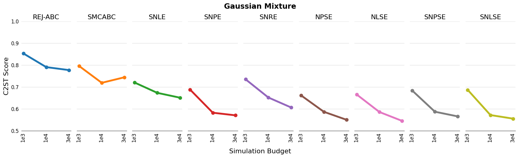
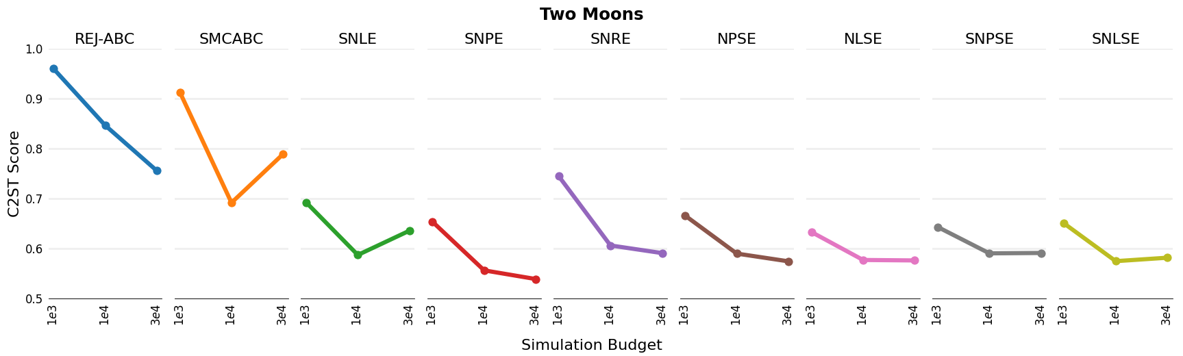
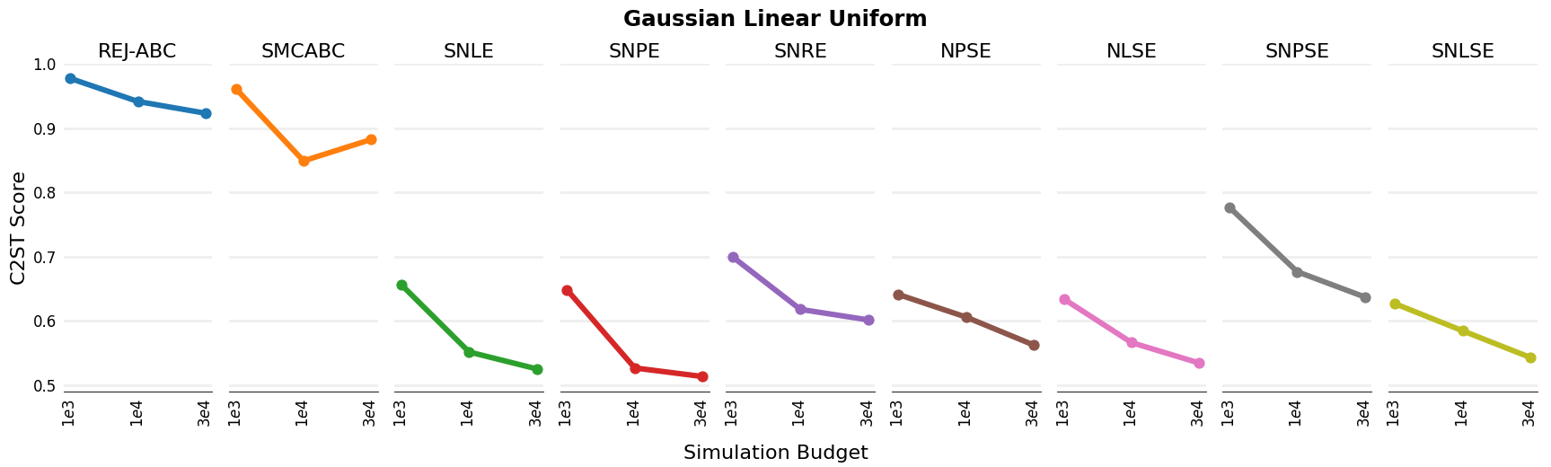
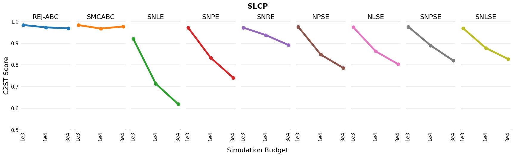
Figure 2: Performance of NPSE, NLSE, SNPSE, and SNLSE on 4 benchmark SBI problems. Each point represents the mean C2ST score (lower is better), computed over ten different observations. For reference, we also show the performance of several existing SBI methods: REJ-ABC, SMC-ABC, SNLE, SNPE, and SNRE.

6 Discussion

6.1 Performance of (S)NLSE and (S)NPSE

Our numerical results demonstrate that conditional score-based diffusion models provide an accurate and robust alternative to existing SBI methods based on density (ratio) estimation (Greenberg et al., 2019; Papamakarios et al., 2019; Hermans et al., 2020). Our amortised, non-sequential methods, NLSE and NPSE, are particularly successful. Indeed, in many cases, these methods can compete with state-of-the-art sequential algorithms such as SNPE, SNLE, and SNRE, which are typically more accurate than their non-sequential counterparts NPE, NLE and NRE (results not shown; see Lueckmann et al., 2021). Our results are particularly impressive for small simulation budgets (see also Figure 1). Indeed, in the majority of our benchmark experiments, our methods outperform all other reference methods given a budget of 1000 simulations.

Empirically, we find that a direct implementation of our sequential methods (SNLSE and SNPSE) may not result in better performance than their non-sequential counterparts (NLSE and NPSE). To remedy this, we scale the score of the proposal priors by a constant $\alpha\in(0,1]$, which is equivalent to generating samples from a tempered proposal prior of $[\hat{p}^{r}(\theta|x_{\text{obs}})]^{\alpha}$. In many cases, this simple modification can lead to significant performance improvements. This being said, we strongly suspect that there are additional modifications which could further improve our sequential methods, allowing them to compete with SNPE and SNLE over a wider range of experiments (e.g., SLCP).

6.2 Likelihood vs Posterior Score Estimation

A natural question is whether it is preferable to estimate the score of the likelihood or the score of the posterior (see also the related discussions in Greenberg et al., 2019; Papamakarios et al., 2019; Lueckmann et al., 2021). In general, the best choice of algorithm will depend on the specific problem at hand. Nonetheless, let us offer some brief thoughts on this question. Our numerical results indicate that, in many cases, estimating the score of the likelihood can lead to slightly more accurate results than estimating the score of the posterior. That is to say, (S)NLSE often slightly outperforms (S)NPSE.

It is worth noting that, in our experiments, it is always possible to compute the perturbed prior analytically, and thus to obtain the score of the perturbed prior using standard auto-differential tools. When this is not possible, NLSE requires us to approximate this term by fitting an additional score network, as do both of our sequential methods. In typical SBI problems, it is extremely cheap to simulate from the prior, particularly in comparison to the simulator. Thus, in principle, one could use as many samples as required to obtain a sufficiently accurate estimate for the prior score. Nonetheless, in such cases, it may be preferable to use NPSE, which only requires us to estimate the posterior score.

Appendix A Computing or Estimating the Perturbed Prior Score

Several of our methods (NLSE, SNPSE, and SNLSE) require us to compute or to estimate the score of the perturbed prior. In this appendix, we provide further details on how to do so.

A.1 Computing the Perturbed Prior Score

For certain choices of the prior, we can obtain the perturbed prior $p_{t}(\theta_{t})=\int_{\mathbb{R}^{d}}p_{t|0}(\theta_{t}|\theta)p(\theta)\mathrm{d}\theta$ in closed form. We can then obtain the score of the perturbed prior $\nabla_{\theta_{t}}\log p_{t}(\theta_{t})$ using automatic differentiation (Bücker et al., 2006). We provide two examples below.

A.1.1 Uniform Prior

Suppose $p(\theta)=\mathcal{U}(\theta|a,b)$ and $p_{t|0}(\theta_{t}|\theta)=\mathcal{N}(\theta_{t}|\theta,\tau_{t}^{2}I)$. We then have

$$p_{t}(\theta_{t}) =\int_{\mathbb{R}^{d}}p(\theta)p_{t|0}(\theta_{t}|\theta)\mathrm{d}\theta$$

$$=\frac{1}{\prod_{i=1}^{d}(b_{i}-a_{i})}\int_{[a_{1},b_{1}]\times\cdots\times[a_{d},b_{d}]}\mathcal{N}(\theta_{t}|\theta,\tau_{t}^{2}I)\mathrm{d}\theta$$

$$=\frac{1}{\prod_{i=1}^{d}(b_{i}-a_{i})}\prod_{i=1}^{d}\left(\Phi(b_{i}|\theta_{t,i},\tau_{i,t}^{2})-\Phi(a_{i}|\theta_{t,i},\tau_{i,t}^{2})\right),$$

where $\Phi(\cdot|\mu,\sigma^{2})$ is the CDF of a univariate Gaussian with mean $\mu$ and variance $\sigma^{2}$.

A.1.2 Gaussian Mixture Prior

Suppose that $p(\theta)=\sum_{i=1}^{n}\alpha_{i}\mathcal{N}(\theta|\mu_{i},\Sigma_{i})$ and $p_{t|0}(\theta_{t}|\theta)=\mathcal{N}(\theta_{t}|\theta,\tau_{t}^{2}I)$. Using standard results (e.g., Equation 2.115 in Bishop, 2006), it follows straightforwardly that

$$p_{t}(\theta_{t}) =\int_{\mathbb{R}^{d}}p(\theta)p_{t|0}(\theta_{t}|\theta)\mathrm{d}\theta$$

$$=\sum_{i=1}^{n}\alpha_{i}\int_{\mathbb{R}^{d}}\mathcal{N}(\theta|\mu_{i},\Sigma_{i})\mathcal{N}(\theta_{t}|\theta,\tau_{t}^{2}I)\mathrm{d}\theta=\sum_{i=1}^{n}\alpha_{i}\mathcal{N}\left(\theta_{t}|\mu_{i},\Sigma_{i}+\tau_{t}^{2}I\right).$$

A.2 Estimating the Perturbed Prior Score

In cases where it is not possible to obtain the perturbed prior in closed form (e.g., if the prior is implicit), we can instead learn an approximation $s_{\psi_{\mathrm{pri}}}(\theta_{t},t)\approx\nabla_{\theta_{t}}\log p_{t}(\theta_{t})$ using score matching. We summarise this procedure below.

Algorithm 2 Prior Score Estimation

  Input: likelihood $p(\theta)$, untrained prior score network $s_{\psi_{\text{pri}}}(\theta_{t},t)$, simulations $N$.

  Output: trained prior score network $\smash{s_{\psi_{\text{pri}}}(\theta_{t},t)\approx\nabla_{\theta_{t}}\log p_{t}(\theta_{t})}$.

  for $i=1:N$ do

     Sample $\theta_{i,0}\sim{p}(\theta)$.

     Sample $(\theta_{i,t})_{t\in(0,T]}\sim p_{t|0}(\theta|\theta_{i,0})$ using the forward diffusion (8).

  end for

  Set $\mathcal{D}=(\theta_{i,0},(\theta_{i,t})_{t\in(0,T]})_{i=1}^{N}$.

  Train $s_{\psi_{\text{pri}}}(\theta_{t},t)\approx\nabla_{\theta}\log{{p}}_{t}(\theta_{t})$ using $\mathcal{D}$,

$$\hat{\mathcal{J}}_{\text{pri}}(\psi_{\text{pri}})=\frac{1}{T}\sum_{t=1}^{T}\frac{1}{N}\sum_{i=1}^{N}\frac{1}{2}\left[\lambda_{t}\left|\left|s_{\psi_{\text{pri}}}(\theta_{i,t},t)-\nabla_{\theta_{t}}\log p_{t|0}(\theta_{i,t}|\theta_{i,0})\right|\right|^{2}\right].\vspace{2mm}$$ (22)

Appendix B Derivations for Neural Posterior Score Estimation (NPSE) and Neural Likelihood Score Estimation (NLSE)

In this appendix, we derive the denoising objective functions used in NPSE and NLSE. We provide these derivations for completeness, noting that similar results can also be found in Batzolis et al. (2021) and Chao et al. (2022), respectively.

B.1 Neural Posterior Score Estimation (NPSE)

In NPSE, the posterior score matching objective function is given by

$$\mathcal{J}_{\mathrm{post}}(\psi_{\mathrm{post}}) =\frac{1}{2}\int_{0}^{T}\lambda_{t}\mathbb{E}_{(\theta_{t},x)\sim p_{t}(\theta_{t},x)}\left[||s_{\psi_{\mathrm{post}}}(\theta_{t},x,t)-\nabla_{\theta_{t}}\log p_{t}(\theta_{t}|x)||^{2}\right]\mathrm{d}t$$

$$=\frac{1}{2}\int_{0}^{T}\lambda_{t}\bigg{[}\underbrace{\mathbb{E}_{(\theta_{t},x)\sim p_{t}(\theta_{t},x)}\big{[}||s_{\psi_{\mathrm{post}}}(\theta_{t},x,t)||^{2}\big{]}}_{\Omega_{t}^{1}}-2\underbrace{\mathbb{E}_{(\theta_{t},x)\sim p_{t}(\theta_{t},x)}[s^{T}_{\psi_{\mathrm{post}}}(\theta_{t},x,t)\nabla_{\theta_{t}}\log p_{t}(\theta_{t}|x)]}_{\Omega_{t}^{2}}$$

$$\hskip 256.0748pt+\underbrace{\mathbb{E}_{(\theta_{t},x)\sim p_{t}(\theta_{t},x)}\big{[}||\nabla_{\theta_{t}}\log p_{t}(\theta_{t}|x)||^{2}\big{]}}_{\Omega_{t}^{3}}\bigg{]}\mathrm{d}t.$$

For the first term $\Omega_{t}^{1}$, we have that

$$\Omega_{t}^{1} =\int_{\mathbb{R}^{d}}\int_{\mathbb{R}^{n}}p_{t}(\theta_{t},x)||s_{\psi_{\mathrm{post}}}(\theta_{t},x,t)||^{2}\mathrm{d}\theta_{t}\mathrm{d}x \mathbb{E}$$ (definition of )

$$=\int_{\mathbb{R}^{d}}\int_{\mathbb{R}^{n}}p_{t}(\theta_{t}|x)p(x)||s_{\psi_{\mathrm{post}}}(\theta_{t},x,t)||^{2}\mathrm{d}\theta_{t}\mathrm{d}x p_{t}(\theta_{t},x)$$ (Bayes’ Theorem for )

$$=\int_{\mathbb{R}^{d}}\int_{\mathbb{R}^{n}}\left[\int_{\mathbb{R}^{n}}p_{t|0}(\theta_{t}|x,\theta_{0})p(\theta_{0}|x)\mathrm{d}\theta_{0}\right]p(x)||s_{\psi_{\mathrm{post}}}(\theta_{t},x,t)||^{2}\mathrm{d}\theta_{t}\mathrm{d}x$$ (law of total probability)

$$=\int_{\mathbb{R}^{d}}\int_{\mathbb{R}^{n}}\int_{\mathbb{R}^{n}}p_{t|0}(\theta_{t}|\theta_{0})p(\theta_{0}|x)p(x)||s_{\psi_{\mathrm{post}}}(\theta_{t},x,t)||^{2}\mathrm{d}\theta_{t}\mathrm{d}\theta_{0}\mathrm{d}x \theta_{t},x|\theta_{0}$$ (conditional independence of )

$$=\mathbb{E}_{(\theta_{0},x)\sim p(\theta_{0},x),\theta_{t}\sim p_{t|0}(\theta_{t}|\theta_{0})}\left[||s_{\psi_{\mathrm{post}}}(\theta_{t},x,t)||^{2}\right]. \mathbb{E}$$ (definition of )

For the second term $\Omega_{t}^{2}$, we have that

$$\Omega_{t}^{2} =\int_{\mathbb{R}^{d}}\int_{\mathbb{R}^{n}}p_{t}(\theta_{t},x)s^{T}_{\psi_{\mathrm{post}}}(\theta_{t},x,t)\nabla_{\theta_{t}}\log p_{t}(\theta_{t}|x)\mathrm{d}\theta_{t}\mathrm{d}x \mathbb{E}$$ (definition of )

$$=\int_{\mathbb{R}^{d}}\int_{\mathbb{R}^{n}}p_{t}(\theta_{t}|x)p(x)s^{T}_{\psi_{\mathrm{post}}}(\theta_{t},x,t)\nabla_{\theta_{t}}\log p_{t}(\theta_{t}|x)\mathrm{d}\theta_{t}\mathrm{d}x p_{t}(\theta_{t},x)$$ (Bayes’ Theorem for )

$$=\int_{\mathbb{R}^{d}}\int_{\mathbb{R}^{n}}p(x)s^{T}_{\psi_{\mathrm{post}}}(\theta_{t},x,t)\nabla_{\theta_{t}}p_{t}(\theta_{t}|x)\mathrm{d}\theta_{t}\mathrm{d}x \nabla_{\theta_{t}}\log p_{t}(\theta_{t}|x)=\frac{\nabla_{\theta_{t}}p_{t}(\theta_{t}|x)}{p_{t}(\theta_{t}|x)}$$ ()

$$=\int_{\mathbb{R}^{d}}\int_{\mathbb{R}^{n}}p(x)s^{T}_{\psi_{\mathrm{post}}}(\theta_{t},x,t)\nabla_{\theta_{t}}\left[\int p_{t|0}(\theta_{t}|x,\theta_{0})p(\theta_{0}|x)\mathrm{d}\theta_{0}\right]\mathrm{d}\theta_{t}\mathrm{d}x$$ (law of total probability)

$$=\int_{\mathbb{R}^{d}}\int_{\mathbb{R}^{n}}\int_{\mathbb{R}^{n}}p(\theta_{0},x)s^{T}_{\psi_{\mathrm{post}}}(\theta_{t},x,t)\nabla_{\theta_{t}}p_{t|0}(\theta_{t}|\theta_{0})\mathrm{d}\theta_{t}\mathrm{d}\theta_{0}\mathrm{d}x \theta_{t},x|\theta_{0}$$ (conditional independence of )

$$=\int_{\mathbb{R}^{d}}\int_{\mathbb{R}^{n}}\int_{\mathbb{R}^{n}}p(\theta_{0},x)p_{t|0}(\theta_{t}|\theta_{0})s^{T}_{\psi_{\mathrm{post}}}(\theta_{t},x,t)\nabla_{\theta_{t}}\log p_{t|0}(\theta_{t}|\theta_{0})\mathrm{d}\theta_{t}\mathrm{d}\theta_{0}\mathrm{d}x \nabla_{\theta_{t}}\log p_{t|0}(\theta_{t}|\theta_{0})=\frac{\nabla_{\theta_{t}}p_{t|0}(\theta_{t}|\theta_{0})}{p_{t|0}(\theta_{t}|\theta_{0})}$$ ()

$$=\mathbb{E}_{(\theta_{0},x)\sim p(\theta_{0},x),\theta_{t}\sim p_{t|0}(\theta_{t}|\theta_{0})}[s^{T}_{\psi_{\mathrm{post}}}(\theta_{t},x,t)\nabla_{\theta_{t}}\log p_{t|0}(\theta_{t}|\theta_{0})]. \mathbb{E}$$ (definition of )

The third term $\Omega_{t}^{3}$ is independent of $\psi_{\text{post}}$. We thus have

$$\mathcal{J}_{\mathrm{post}}(\psi_{\mathrm{post}}) \propto\frac{1}{2}\int_{0}^{t}\lambda_{t}\mathbb{E}_{(\theta_{0},x)\sim p(\theta_{0},x),\theta_{t}\sim p_{t|0}(\theta_{t}|\theta_{0})}\left[||s_{\psi_{\mathrm{post}}}(\theta_{t},x,t)||^{2}-2s^{T}_{\psi_{\mathrm{post}}}(\theta_{t},x,t)\nabla_{\theta_{t}}\log p_{t|0}(\theta_{t}|\theta_{0})\right]$$

$$\propto\frac{1}{2}\int_{0}^{t}\lambda_{t}\mathbb{E}_{(\theta_{0},x)\sim p(\theta_{0},x),\theta_{t}\sim p_{t|0}(\theta_{t}|\theta_{0})}\left[||s_{\psi_{\mathrm{post}}}(\theta_{t},x,t)-\nabla_{\theta_{t}}\log p_{t|0}(\theta_{t}|\theta_{0})||^{2}\right]\mathrm{d}t.$$

B.2 Neural Likelihood Score Estimation (NLSE)

In NLSE, we have two score-matching objective functions: one for the prior, and one for the likelihood. We will derive each of these in turn.

B.2.1 Prior

The prior score matching objective function is given by

$$\mathcal{J}_{\mathrm{pri}}(\psi_{\mathrm{pri}}) =\frac{1}{2}\int_{0}^{T}\lambda_{t}\mathbb{E}_{\theta_{t}\sim p_{t}(\theta_{t})}\left[||s_{\psi_{\mathrm{pri}}}(\theta_{t},t)-\nabla_{\theta_{t}}\log p_{t}(\theta_{t})||^{2}\right]\mathrm{d}t$$

$$=\frac{1}{2}\int_{0}^{T}\lambda_{t}\bigg{[}\underbrace{\mathbb{E}_{\theta_{t}\sim p_{t}(\theta_{t})}[||s_{\psi_{\mathrm{pri}}}(\theta_{t},t)||^{2}]}_{\Omega_{t}^{1}}-2\underbrace{\mathbb{E}_{\theta_{t}\sim p_{t}(\theta_{t})}[s^{T}_{\psi_{\mathrm{pri}}}(\theta_{t},t)\nabla_{\theta_{t}}\log p_{t}(\theta_{t})}_{\Omega_{t}^{2}}]+\underbrace{\mathbb{E}_{\theta_{t}\sim p_{t}(\theta_{t})}[||\nabla_{\theta_{t}}\log p_{t}(\theta_{t})||^{2}]}_{\Omega_{t}^{3}}\bigg{]}\mathrm{d}t.$$

We will simplify these terms using essentially identical arguments to those given in the previous section. In particular, we have

$$\Omega_{t}^{1} =\int_{\mathbb{R}^{n}}p_{t}(\theta_{t})||s_{\psi_{\mathrm{pri}}}(\theta_{t},t)||^{2}\mathrm{d}\theta_{t} \mathbb{E}$$ (definition of )

$$=\int_{\mathbb{R}^{n}}\int_{\mathbb{R}^{n}}p_{t|0}(\theta_{t}|\theta_{0})p(\theta_{0})||s_{\psi_{\mathrm{pri}}}(\theta_{t},t)||^{2}\mathrm{d}\theta_{t}\mathrm{d}\theta_{0}$$ (law of total probability)

$$=\mathbb{E}_{\theta_{0}\sim p(\theta_{0}),\theta_{t}\sim p_{t|0}(\theta_{t}|\theta_{0})}\left[||s_{\psi_{\mathrm{pri}}}(\theta_{t},t)||^{2}\right], \mathbb{E}$$ (definition of )

$$\Omega_{t}^{2} =\int_{\mathbb{R}^{n}}p_{t}(\theta_{t})s^{T}_{\psi_{\mathrm{pri}}}(\theta_{t},t)\nabla_{\theta_{t}}\log p_{t}(\theta_{t})\mathrm{d}\theta_{t} \mathbb{E}$$ (definition of )

$$=\int_{\mathbb{R}^{n}}s^{T}_{\psi_{\mathrm{pri}}}(\theta_{t},t)\nabla_{\theta_{t}}p_{t}(\theta_{t})\mathrm{d}\theta_{t} \nabla_{\theta_{t}}\log p_{t}(\theta_{t})=\frac{\nabla_{\theta_{t}}p_{t}(\theta_{t})}{p_{t}(\theta_{t})}$$ ()

$$=\int_{\mathbb{R}^{n}}s^{T}_{\psi_{\mathrm{pri}}}(\theta_{t},t)\nabla_{\theta_{t}}\left[\int_{\mathbb{R}^{n}}p_{t|0}(\theta_{t}|\theta_{0})p(\theta_{0})\mathrm{d}\theta_{0}\right]\mathrm{d}\theta_{t}$$ (law of total probability)

$$=\int_{\mathbb{R}^{n}}\int_{\mathbb{R}^{n}}p_{t|0}(\theta_{t}|\theta_{0})p(\theta_{0})s^{T}_{\psi_{\mathrm{pri}}}(\theta_{t},t)\nabla_{\theta_{t}}\log p_{t|0}(\theta_{t}|\theta_{0})\mathrm{d}\theta_{0}\mathrm{d}\theta_{t} \nabla_{\theta_{t}}\log p_{t}(\theta_{t})=\frac{\nabla_{\theta_{t}}p_{t}(\theta_{t})}{p_{t}(\theta_{t})}$$ ()

$$=\mathbb{E}_{\theta_{0}\sim p(\theta_{0})\theta\sim p_{t|0}(\theta_{t}|\theta_{0})}[s^{T}_{\psi_{\mathrm{pri}}}(\theta_{t},t)\nabla_{\theta_{t}}\log p_{t|0}(\theta_{t}|\theta_{0})], \mathbb{E}$$ (definition of )

and that $\Omega_{t}^{3}$ is independent of $\psi_{\text{pri}}$. Thus, arguing as before, we have

$$\mathcal{J}_{\text{pri}}(\psi_{\text{pri}}) \propto\frac{1}{2}\int_{0}^{T}\lambda_{t}\mathbb{E}_{\theta_{0}\sim p(\theta_{0})\theta\sim p_{t|0}(\theta_{t}|\theta_{0})}\left[||s_{\psi_{\mathrm{pri}}}(\theta_{t},t)||^{2}-2s^{T}_{\psi_{\mathrm{pri}}}(\theta_{t},t)\nabla_{\theta_{t}}\log p_{t|0}(\theta_{t}|\theta_{0})\right]\mathrm{d}t$$

$$\propto\frac{1}{2}\int_{0}^{T}\lambda_{t}\mathbb{E}_{\theta_{0}\sim p(\theta_{0})\theta\sim p_{t|0}(\theta_{t}|\theta_{0})}\left[||s_{\psi_{\mathrm{pri}}}(\theta_{t},t)-\nabla_{\theta_{t}}\log p_{t|0}(\theta_{t}|\theta_{0})||^{2}\right]\mathrm{d}t.$$

B.2.2 Likelihood

The likelihood score matching objective function is given by

$$\mathcal{J}_{\mathrm{lik}}(\psi_{\mathrm{lik}}) =\frac{1}{2}\int_{0}^{T}\lambda_{t}\mathbb{E}_{(\theta_{t},x)\sim p_{t}(\theta_{t},x)}\left[||s_{\psi_{\mathrm{lik}}}(\theta_{t},x,t)-\nabla_{\theta_{t}}\log p_{t}(x|\theta_{t})||^{2}\right]\mathrm{d}t$$

$$=\frac{1}{2}\int_{0}^{T}\lambda_{t}\bigg{[}\underbrace{\mathbb{E}_{(\theta_{t},x)\sim p_{t}(\theta_{t},x)}[||s_{\psi_{\mathrm{lik}}}(\theta_{t},x,t)||^{2}}_{\Omega_{t}^{1}}-2\underbrace{\mathbb{E}_{(\theta_{t},x)\sim p_{t}(\theta_{t},x)}[s^{T}_{\psi_{\mathrm{lik}}}(\theta_{t},x,t)\nabla_{\theta_{t}}\log p_{t}(x|\theta_{t})]}_{\Omega_{t}^{2}}$$

$$\hskip 233.31259pt+\underbrace{\mathbb{E}_{(\theta_{t},x)\sim p_{t}(\theta_{t},x)}[||\nabla_{\theta_{t}}\log p_{t}(x|\theta_{t})||^{2}]}_{\Omega_{t}^{3}}\bigg{]}\mathrm{d}t.$$

We now proceed in much the same vein as before. On this occasion, leveraging the same arguments as in Appendix B.1, it is straightforward to obtain

$$\Omega_{t}^{1} =\int_{\mathbb{R}^{d}}\int_{\mathbb{R}^{n}}p_{t}(\theta_{t},x)||s_{\psi_{\mathrm{lik}}}(\theta_{t},x,t)||^{2}\mathrm{d}\theta_{t}\mathrm{d}x \mathbb{E}$$ (definition of )

$$=\mathbb{E}_{(\theta_{0},x)\sim p(\theta_{0},x),\theta_{t}\sim p_{t|0}(\theta_{t}|\theta_{0})}\left[||s_{\psi_{\mathrm{lik}}}(\theta_{t},x,t)||^{2}\right], \Omega_{t}^{1}$$ (identically to in Appendix B.1)

$$\Omega_{t}^{2} =\int_{\mathbb{R}^{d}}\int_{\mathbb{R}^{n}}p_{t}(\theta_{t},x)s^{T}_{\psi_{\mathrm{lik}}}(\theta_{t},x,t)\nabla_{\theta_{t}}\log p_{t}(x|\theta_{t})\mathrm{d}\theta_{t}\mathrm{d}x \mathbb{E}$$ (definition of )

$$=\int_{\mathbb{R}^{d}}\int_{\mathbb{R}^{n}}p_{t}(\theta_{t},x)s^{T}_{\psi_{\mathrm{lik}}}(\theta_{t},x,t)[\nabla_{\theta_{t}}\log p_{t}(\theta_{t}|x)-\nabla_{\theta_{t}}\log p_{t}(\theta_{t})]\mathrm{d}\theta_{t}\mathrm{d}x$$ (Bayes’ Theorem)

$$=\mathbb{E}_{(\theta_{0},x)\sim p(\theta_{0},x),\theta\sim p_{t|0}(\theta_{t}|\theta_{0})}\left[s^{T}_{\psi_{\mathrm{lik}}}(\theta_{t},x,t)\nabla_{\theta_{t}}\log p_{t|0}(\theta_{t}|\theta_{0})-s^{T}_{\psi_{\mathrm{lik}}}(\theta_{t},x,t)\nabla_{\theta_{t}}\log p_{t}(\theta_{t})\right],$$ (from Appendix B.1)

and, of course, that $\Omega_{t}^{3}$ is independent of $\psi_{\mathrm{lik}}$. Putting everything together, we thus have

$$\mathcal{J}_{\mathrm{lik}}(\psi_{\mathrm{lik}}) \propto\frac{1}{2}\int_{0}^{T}\lambda_{t}\mathbb{E}_{(\theta_{0},x)\sim p(\theta_{0},x),\theta\sim p_{t|0}(\theta_{t}|\theta_{0})}\big{[}||s_{\psi_{\mathrm{lik}}}(\theta_{t},x,t)||^{2}-2s^{T}_{\psi_{\mathrm{lik}}}(\theta_{t},x,t)\nabla_{\theta_{t}}\log p_{t|0}(\theta_{t}|\theta_{0})$$

$$\hskip 247.53897pt+2s^{T}_{\psi_{\mathrm{lik}}}(\theta_{t},x,t)\nabla_{\theta_{t}}\log p_{t}(\theta_{t})\big{]}\mathrm{d}t$$

$$\propto\frac{1}{2}\int_{0}^{T}\lambda_{t}\mathbb{E}_{(\theta_{0},x)\sim p(\theta_{0},x),\theta\sim p_{t|0}(\theta_{t}|\theta_{0})}\left[||s_{\psi_{\mathrm{lik}}}(\theta_{t},x,t)-\left(\nabla_{\theta_{t}}\log p_{t|0}(\theta_{t}|\theta_{0})-\nabla_{\theta_{t}}\log p_{t}(\theta_{t})\right)||^{2}\right]\mathrm{d}t.$$

Appendix C Derivations for Sequential Neural Posterior Score Estimation (SNPSE) and Sequential Neural Likelihood Estimation (SNLSE)

We now derive the objective functions used in sequential neural posterior estimation (SNPSE) and sequential neural likelihood estimation (SNLSE). In this section, as in the main text, we will use the notation $\tilde{p}^{r}_{t}(\theta_{t})=\frac{1}{r}\sum_{s=0}^{r-1}\hat{p}_{t}^{s}(\theta_{t}|x_{\text{obs}})$ to denote the (perturbed) proposal prior in round $r$. We will often also write $\hat{p}_{t}^{s}(\theta_{t}):=\hat{p}_{t}^{s}(\theta_{t}|x_{\text{obs}})$ for the proposal prior components, dropping the dependence on $x_{\text{obs}}$ for ease of notation.

C.1 Sequential Neural Posterior Score Estimation (SNPSE)

In SNPSE, the posterior score-matching objective function in round $r$ is given by

$$\mathcal{J}^{r}_{\mathrm{post}}(\psi_{\mathrm{post}}) =\frac{1}{2}\int_{0}^{T}\lambda_{t}\mathbb{E}_{(\theta_{t},x)\sim\tilde{p}^{r}_{t}(\theta_{t},x)}\left[||s_{\psi_{\mathrm{post}}}(\theta_{t},x,t)-\nabla_{\theta_{t}}\log p_{t}(\theta_{t}|x)||^{2}\right]\mathrm{d}t$$

$$=\frac{1}{2}\int_{0}^{T}\lambda_{t}\bigg{[}\underbrace{\mathbb{E}_{(\theta_{t},x)\sim\tilde{p}^{r}_{t}(\theta_{t},x)}[||s_{\psi_{\mathrm{post}}}(\theta_{t},x,t)||^{2}]}_{\Omega_{t}^{1}}-2\underbrace{\mathbb{E}_{(\theta_{t},x)\sim\tilde{p}^{r}_{t}(\theta_{t},x)}[s^{T}_{\psi_{\mathrm{post}}}(\theta_{t},x,t)\nabla_{\theta_{t}}\log p_{t}(\theta_{t}|x)]}_{\Omega_{t}^{2}}$$

$$\hskip 250.38425pt+\underbrace{\mathbb{E}_{(\theta_{t},x)\sim\tilde{p}^{r}_{t}(\theta_{t},x)}[||\nabla_{\theta_{t}}\log p_{t}(\theta_{t}|x)||^{2}]}_{\Omega_{t}^{3}}\bigg{]}\mathrm{d}t.$$

For the first term $\Omega_{t}^{1}$, we have

$$\Omega_{t}^{1} =\int_{\mathbb{R}^{d}}\int_{\mathbb{R}^{n}}\tilde{p}_{t}^{r}(\theta_{t},x)||s_{\psi_{\mathrm{post}}}(\theta_{t},x,t)||^{2}\mathrm{d}\theta_{t}\mathrm{d}x \mathbb{E}$$ (definition of )

$$=\int_{\mathbb{R}^{d}}\int_{\mathbb{R}^{n}}p_{t}(x|\theta_{t})\tilde{p}_{t}^{r}(\theta_{t})||s_{\psi_{\mathrm{post}}}(\theta_{t},x,t)||^{2}\mathrm{d}\theta_{t}\mathrm{d}x \tilde{p}_{t}^{r}(\theta_{t},x)$$ (Bayes’ Theorem for )

$$=\int_{\mathbb{R}^{d}}\int_{\mathbb{R}^{n}}p_{t}(x|\theta_{t})\left[\frac{1}{r}\sum_{s=0}^{r-1}\hat{p}_{t}^{s}(\theta_{t})\right]||s_{\psi_{\mathrm{post}}}(\theta_{t},x,t)||^{2}\mathrm{d}\theta_{t}\mathrm{d}x \tilde{p}_{t}^{r}(\theta_{t})$$ (definition of )

$$=\frac{1}{r}\sum_{s=0}^{r-1}\int_{\mathbb{R}^{d}}\int_{\mathbb{R}^{n}}\hat{p}^{s}_{t}(\theta_{t},x)||s_{\psi_{\mathrm{post}}}(\theta_{t},x,t)||^{2}\mathrm{d}\theta_{t}\mathrm{d}x p_{t}(x|\theta_{t})$$ (Bayes’ Theorem for )

$$=\frac{1}{r}\sum_{s=0}^{r-1}\int_{\mathbb{R}^{d}}\int_{\mathbb{R}^{n}}\hat{p}^{s}(x)\hat{p}_{t}^{s}(\theta_{t}|x)||s_{\psi_{\mathrm{post}}}(\theta_{t},x,t)||^{2}\mathrm{d}\theta_{t}\mathrm{d}x \hat{p}_{t}^{s}(\theta_{t},x)$$ (Bayes’ Theorem for )

$$=\frac{1}{r}\sum_{s=0}^{r-1}\int_{\mathbb{R}^{d}}\int_{\mathbb{R}^{n}}\hat{p}^{s}(x)\left[\int\hat{p}_{t|0}^{s}(\theta_{t}|\theta_{0},x)\hat{p}^{s}(\theta_{0}|x)\mathrm{d}\theta_{0}\right]||s_{\psi_{\mathrm{post}}}(\theta_{t},x,t)||^{2}\mathrm{d}\theta_{t}\mathrm{d}x$$ (law of total probability)

$$=\frac{1}{r}\sum_{s=0}^{r-1}\int_{\mathbb{R}^{d}}\int_{\mathbb{R}^{n}}\hat{p}^{s}(x)\left[\int p_{t|0}(\theta_{t}|\theta_{0})\hat{p}^{s}(\theta_{0}|x)\mathrm{d}\theta_{0}\right]||s_{\psi_{\mathrm{post}}}(\theta_{t},x,t)||^{2}\mathrm{d}\theta_{t}\mathrm{d}x \theta_{t},x|\theta_{0}$$ (conditional independence of )

$$=\frac{1}{r}\sum_{s=0}^{r-1}\int_{\mathbb{R}^{d}}\int_{\mathbb{R}^{n}}\int_{\mathbb{R}^{n}}\hat{p}^{s}(\theta_{0})p(x|\theta_{0})p_{t|0}(\theta_{t}|\theta_{0})||s_{\psi_{\mathrm{post}}}(\theta_{t},x,t)||^{2}\mathrm{d}\theta_{t}\mathrm{d}\theta_{0}\mathrm{d}x \hat{p}^{s}(\theta_{0}|x)$$ (Bayes’ Theorem for )

$$=\frac{1}{r}\sum_{s=0}^{r-1}\mathbb{E}_{(\theta_{0},x)\sim\hat{p}^{s}(\theta_{0})p(x|\theta_{0}),\theta_{t}\sim p_{t|0}(\theta_{t}|\theta_{0})}\left[||s_{\psi_{\mathrm{post}}}(\theta_{t},x,t)||^{2}\right] \mathbb{E}$$ (definition of ).

We note that, in the final five lines, we have established that

$$\int\int\hat{p}_{t}^{s}(\theta_{t},x)[\cdots]\mathrm{d}\theta_{t}\mathrm{d}x=\int\int\int\hat{p}^{s}(\theta_{0})p(x|\theta_{0})p_{t|0}(\theta_{t}|\theta_{0})[\cdots]\mathrm{d}\theta_{t}\mathrm{d}x\mathrm{d}\theta_{0}.$$ (23)

We will frequently re-use this identity in our subsequent calculations.

We now turn our attention to the second term $\Omega_{t}^{2}$. Using the decomposition given in (18), we have

$$\Omega_{t}^{2} =\underbrace{\mathbb{E}_{(\theta_{t},x)\sim\tilde{p}^{r}_{t}(\theta_{t},x)}\left[s^{T}_{\psi_{\mathrm{post}}}(\theta_{t},x,t)\nabla_{\theta_{t}}\log\tilde{p}_{t}^{r}(\theta_{t}|x)\right]}_{\Omega_{t}^{2,1}}$$

$$~{}+\underbrace{\mathbb{E}_{(\theta_{t},x)\sim\tilde{p}^{r}_{t}(\theta_{t},x)}[s^{T}_{\psi_{\mathrm{post}}}(\theta_{t},x,t)\nabla_{\theta_{t}}\log\tilde{p}_{t}^{r}(\theta_{t})]}_{\Omega_{t}^{2,2}}-\underbrace{\mathbb{E}_{(\theta_{t},x)\sim\tilde{p}^{r}_{t}(\theta_{t},x)}[s^{T}_{\psi_{\mathrm{post}}}(\theta_{t},x,t)\nabla_{\theta_{t}}\log{p}_{t}(\theta_{t})]}_{\Omega_{t}^{2,3}}.$$

We will deal with these three quantities in turn. For the first term, we have

$$\Omega_{t}^{2,1} =\int_{\mathbb{R}^{d}}\int_{\mathbb{R}^{n}}\tilde{p}_{t}^{r}(\theta_{t},x)s^{T}_{\psi_{\mathrm{post}}}(\theta_{t},x,t)\nabla_{\theta_{t}}\log\tilde{p}^{r}_{t}(\theta_{t}|x)\mathrm{d}\theta_{t}\mathrm{d}x \mathbb{E}$$ (definition of )

$$=\int_{\mathbb{R}^{d}}\int_{\mathbb{R}^{n}}\tilde{p}_{t}^{r}(\theta_{t},x)s^{T}_{\psi_{\mathrm{post}}}(\theta_{t},x,t)\nabla_{\theta_{t}}\log\tilde{p}^{r}_{t}(\theta_{t},x)\mathrm{d}\theta_{t}\mathrm{d}x \nabla_{\theta_{t}}\log\tilde{p}^{r}_{t}(\theta_{t}|x)=\nabla_{\theta_{t}}\log\tilde{p}^{r}_{t}(\theta_{t},x)$$ ()

$$=\int_{\mathbb{R}^{d}}\int_{\mathbb{R}^{n}}s^{T}_{\psi_{\mathrm{post}}}(\theta_{t},x,t)\nabla_{\theta_{t}}\tilde{p}^{r}_{t}(\theta_{t},x)\mathrm{d}\theta_{t}\mathrm{d}x \nabla_{\theta_{t}}\log\tilde{p}^{r}_{t}(\theta_{t},x)=\frac{\nabla_{\theta_{t}}\tilde{p}^{r}_{t}(\theta_{t},x)}{\tilde{p}^{r}_{t}(\theta_{t},x)}$$ ()

$$=\int_{\mathbb{R}^{d}}\int_{\mathbb{R}^{n}}s^{T}_{\psi_{\mathrm{post}}}(\theta_{t},x,t)\nabla_{\theta_{t}}\left[\tilde{p}^{r}_{t}(\theta_{t})p_{t}(x|\theta_{t})\right]\mathrm{d}\theta_{t}\mathrm{d}x \tilde{p}^{r}_{t}(\theta_{t},x)$$ (Bayes’ Theorem for )

$$=\int_{\mathbb{R}^{d}}\int_{\mathbb{R}^{n}}s^{T}_{\psi_{\mathrm{post}}}(\theta_{t},x,t)\nabla_{\theta_{t}}\left[\frac{1}{r}\sum_{s=0}^{r-1}\hat{p}^{s}_{t}(\theta_{t})p_{t}(x|\theta_{t})\right]\mathrm{d}\theta_{t}\mathrm{d}x \tilde{p}_{t}^{r}(\theta_{t})$$ (definition of )

$$=\frac{1}{r}\sum_{s=0}^{r-1}\int_{\mathbb{R}^{d}}\int_{\mathbb{R}^{n}}s^{T}_{\psi_{\mathrm{post}}}(\theta_{t},x,t)\nabla_{\theta_{t}}\left[\hat{p}^{s}_{t}(\theta_{t}|x)\hat{p}^{s}(x)\right]\mathrm{d}\theta_{t}\mathrm{d}x \hat{p}^{s}_{t}(\theta_{t},x)$$ (Bayes’ Theorem for )

$$=\frac{1}{r}\sum_{s=0}^{r-1}\int_{\mathbb{R}^{d}}\int_{\mathbb{R}^{n}}s^{T}_{\psi_{\mathrm{post}}}(\theta_{t},x,t)\nabla_{\theta_{t}}\left[\int_{\mathbb{R}^{n}}\hat{p}^{s}_{t|0}(\theta_{t}|x,\theta_{0})\hat{p}^{s}(\theta_{0}|x)\mathrm{d}\theta_{0}\right]\hat{p}^{s}(x)\mathrm{d}\theta_{t}\mathrm{d}x$$ (law of total probability)

$$=\frac{1}{r}\sum_{s=0}^{r-1}\int_{\mathbb{R}^{d}}\int_{\mathbb{R}^{n}}s^{T}_{\psi_{\mathrm{post}}}(\theta_{t},x,t)\nabla_{\theta_{t}}\left[\int_{\mathbb{R}^{n}}p_{t|0}(\theta_{t}|\theta_{0})\hat{p}^{s}(\theta_{0}|x)\mathrm{d}\theta_{0}\right]\hat{p}^{s}(x)\mathrm{d}\theta_{t}\mathrm{d}x \theta_{t},x|\theta_{0}$$ (conditional independence of )

$$=\frac{1}{r}\sum_{s=0}^{r-1}\int_{\mathbb{R}^{d}}\int_{\mathbb{R}^{n}}\int_{\mathbb{R}^{n}}s^{T}_{\psi_{\mathrm{post}}}(\theta_{t},x,t)\nabla_{\theta_{t}}\left[p_{t|0}(\theta_{t}|\theta_{0})\right]\hat{p}^{s}(\theta_{0}|x)\hat{p}^{s}(x)\mathrm{d}\theta_{t}\mathrm{d}\theta_{0}\mathrm{d}x$$ (interchange the integral and the derivative)

$$=\frac{1}{r}\sum_{s=0}^{r-1}\int_{\mathbb{R}^{d}}\int_{\mathbb{R}^{n}}\int_{\mathbb{R}^{n}}p_{t|0}(\theta_{t}|\theta_{0})\hat{p}^{s}(\theta_{0}|x)\hat{p}^{s}(x)s^{T}_{\psi_{\mathrm{post}}}(\theta_{t},x,t)\nabla_{\theta_{t}}\log p_{t|0}(\theta_{t}|\theta_{0})\mathrm{d}\theta_{t}\mathrm{d}\theta_{0}\mathrm{d}x \nabla_{\theta_{t}}\log{p}_{t|0}(\theta_{t}|\theta_{0})=\frac{\nabla_{\theta_{t}}{p}_{t|0}(\theta_{t}|\theta_{0})}{\tilde{p}_{t|0}(\theta_{t}|\theta_{0})}$$ ()

$$=\frac{1}{r}\sum_{s=0}^{r-1}\mathbb{E}_{(\theta_{0},x)\sim\hat{p}^{s}(\theta_{0})p(x|\theta_{0}),\theta_{t}\sim p_{t|0}(\theta_{t}|\theta_{0})}\left[s^{T}_{\psi_{\mathrm{post}}}(\theta_{t},x,t)\nabla_{\theta_{t}}\log p_{t|0}(\theta_{t}|\theta_{0})\right] \mathbb{E}$$ (definition of ).

Meanwhile, for the second term we can compute

$$\Omega_{t}^{2,2} =\int_{\mathbb{R}^{d}}\int_{\mathbb{R}^{n}}\tilde{p}_{t}^{r}(\theta_{t},x)s^{T}_{\psi_{\mathrm{post}}}(\theta_{t},x,t)\nabla_{\theta_{t}}\log\tilde{p}^{r}_{t}(\theta_{t})\mathrm{d}\theta_{t}\mathrm{d}x \mathbb{E}$$ (definition of )

$$=\int_{\mathbb{R}^{d}}\int_{\mathbb{R}^{n}}\tilde{p}_{t}^{r}(\theta_{t})p_{t}(x|\theta_{t})s^{T}_{\psi_{\mathrm{post}}}(\theta_{t},x,t)\nabla_{\theta_{t}}\log\tilde{p}^{r}_{t}(\theta_{t})\mathrm{d}\theta_{t}\mathrm{d}x \tilde{p}_{t}^{r}(\theta_{t},x)$$ (Bayes’ Theorem for )

$$=\int_{\mathbb{R}^{d}}\int_{\mathbb{R}^{n}}p_{t}(x|\theta_{t})s^{T}_{\psi_{\mathrm{post}}}(\theta_{t},x,t)\nabla_{\theta_{t}}\tilde{p}^{r}_{t}(\theta_{t})\mathrm{d}\theta_{t}\mathrm{d}x \nabla_{\theta_{t}}\log\tilde{p}^{r}_{t}(\theta_{t})=\frac{\nabla_{\theta_{t}}\tilde{p}^{r}_{t}(\theta_{t})}{\tilde{p}^{r}_{t}(\theta_{t})}$$ ()

$$=\int_{\mathbb{R}^{d}}\int_{\mathbb{R}^{n}}p_{t}(x|\theta_{t})s^{T}_{\psi_{\mathrm{post}}}(\theta_{t},x,t)\nabla_{\theta_{t}}\left[\frac{1}{r}\sum_{s=0}^{r-1}\hat{p}^{s}_{t}(\theta_{t})\right]\mathrm{d}\theta_{t}\mathrm{d}x \tilde{p}_{t}^{r}(\theta_{t})$$ (definition of )

$$=\frac{1}{r}\sum_{s=0}^{r-1}\int_{\mathbb{R}^{d}}\int_{\mathbb{R}^{n}}p_{t}(x|\theta_{t})s^{T}_{\psi_{\mathrm{post}}}(\theta_{t},x,t)\nabla_{\theta_{t}}\hat{p}^{s}_{t}(\theta_{t})\mathrm{d}\theta_{t}\mathrm{d}x$$ (interchange the sum and the derivative)

$$=\frac{1}{r}\sum_{s=0}^{r-1}\int_{\mathbb{R}^{d}}\int_{\mathbb{R}^{n}}\hat{p}^{s}_{t}(\theta_{t})p_{t}(x|\theta_{t})s^{T}_{\psi_{\mathrm{post}}}(\theta_{t},x,t)\nabla_{\theta_{t}}\log\hat{p}^{s}_{t}(\theta_{t})\mathrm{d}\theta_{t}\mathrm{d}x \nabla_{\theta_{t}}\log\hat{p}^{s}_{t}(\theta_{t})=\frac{\nabla_{\theta_{t}}\hat{p}^{s}_{t}(\theta_{t})}{\hat{p}^{s}_{t}(\theta_{t})}$$ ()

$$=\frac{1}{r}\sum_{s=0}^{r-1}\int_{\mathbb{R}^{d}}\int_{\mathbb{R}^{n}}\hat{p}^{s}_{t}(\theta_{t},x)s^{T}_{\psi_{\mathrm{post}}}(\theta_{t},x,t)\nabla_{\theta_{t}}\log\hat{p}^{s}_{t}(\theta_{t})\mathrm{d}\theta_{t}\mathrm{d}x \hat{p}_{t}^{s}(\theta_{t},x)$$ (Bayes’ Theorem for )

$$=\frac{1}{r}\sum_{s=0}^{r-1}\int_{\mathbb{R}^{d}}\int_{\mathbb{R}^{n}}\int_{\mathbb{R}^{n}}\hat{p}^{s}(\theta_{0})p(x|\theta_{0})p_{t|0}(\theta_{t}|\theta_{0})s^{T}_{\psi_{\mathrm{post}}}(\theta_{t},x,t)\nabla_{\theta_{t}}\log\hat{p}^{s}_{t}(\theta_{t})\mathrm{d}\theta_{t}\mathrm{d}x$$ (Equation (23))

$$=\frac{1}{r}\sum_{s=0}^{r-1}\mathbb{E}_{(\theta_{0},x)\sim\hat{p}^{s}(\theta_{0})p(x|\theta_{0}),\theta_{t}\sim p_{t|0}(\theta_{t}|\theta_{0})}\left[s^{T}_{\psi_{\mathrm{post}}}(\theta_{t},x,t)\nabla_{\theta_{t}}\log\hat{p}^{s}_{t}(\theta_{t})\right] \mathbb{E}$$ (definition of ).

Finally, for the third term, we have

$$\Omega_{t}^{2,3} =\int_{\mathbb{R}^{d}}\int_{\mathbb{R}^{n}}\tilde{p}_{t}^{r}(\theta_{t},x)s^{T}_{\psi_{\mathrm{post}}}(\theta_{t},x,t)\nabla_{\theta_{t}}\log p_{t}(\theta_{t})\mathrm{d}\theta_{t}\mathrm{d}x \mathbb{E}$$ (definition of )

$$=\int_{\mathbb{R}^{d}}\int_{\mathbb{R}^{n}}p_{t}(x|\theta_{t})\tilde{p}_{t}^{r}(\theta_{t})s^{T}_{\psi_{\mathrm{post}}}(\theta_{t},x,t)\nabla_{\theta_{t}}\log p_{t}(\theta_{t})\mathrm{d}\theta_{t}\mathrm{d}x \tilde{p}_{t}^{r}(\theta_{t},x)$$ (Bayes’ Theorem for )

$$=\int_{\mathbb{R}^{d}}\int_{\mathbb{R}^{n}}p_{t}(x|\theta_{t})\left[\frac{1}{r}\sum_{s=0}^{r-1}\hat{p}_{t}^{s}(\theta_{t})\right]s^{T}_{\psi_{\mathrm{post}}}(\theta_{t},x,t)\nabla_{\theta_{t}}\log p_{t}(\theta_{t})\mathrm{d}\theta_{t}\mathrm{d}x \tilde{p}_{t}^{r}(\theta_{t})$$ (definition of )

$$=\frac{1}{r}\sum_{s=0}^{r-1}\int_{\mathbb{R}^{d}}\int_{\mathbb{R}^{n}}\hat{p}_{t}^{s}(\theta_{t},x)s^{T}_{\psi_{\mathrm{post}}}(\theta_{t},x,t)\nabla_{\theta_{t}}\log p_{t}(\theta_{t})\mathrm{d}\theta_{t}\mathrm{d}x \hat{p}_{t}^{s}(\theta_{t},x)$$ (Bayes’ Theorem for )

$$=\frac{1}{r}\sum_{s=0}^{r-1}\int_{\mathbb{R}^{d}}\int_{\mathbb{R}^{n}}\int_{\mathbb{R}^{n}}\hat{p}^{s}(\theta_{0}){p}(x|\theta_{0})p_{t|0}(\theta_{t}|\theta_{0})s^{T}_{\psi_{\mathrm{post}}}(\theta_{t},x,t)\nabla_{\theta_{t}}\log p_{t}(\theta_{t})\mathrm{d}\theta_{t}\mathrm{d}\theta_{0}\mathrm{d}x$$ (Equation (23))

$$=\frac{1}{r}\sum_{s=0}^{r-1}\mathbb{E}_{(\theta_{0},x)\sim\hat{p}^{s}(\theta_{0})p(x|\theta_{0}),\theta_{t}\sim p_{t|0}(\theta_{t}|\theta_{0})}\left[s^{T}_{\psi_{\mathrm{post}}}(\theta_{t},x,t)\nabla_{\theta_{t}}\log p_{t}(\theta_{t})\right] \mathbb{E}$$ (definition of ).

Putting everything together, we finally arrive at

$$\mathcal{J}^{r}_{\mathrm{post}}(\psi_{\mathrm{post}}) \propto\frac{1}{r}\sum_{s=0}^{r-1}\frac{1}{2}\int_{0}^{T}\lambda_{t}\mathbb{E}_{(\theta_{0},x)\sim\hat{p}^{s}(\theta_{0})p(x|\theta_{0}),\theta_{t}\sim p_{t|0}(\theta_{t}|\theta_{0})}\bigg{[}||s_{\psi_{\mathrm{post}}}(\theta_{t},x,t)||^{2}$$

$$\hskip 113.81102pt-2s^{T}_{\psi_{\mathrm{post}}}(\theta_{t},x,t)\left[\nabla_{\theta_{t}}\log p_{t|0}(\theta_{t}|\theta_{0})-\nabla_{\theta_{t}}\log p_{t}^{s}(\theta_{t})+\nabla_{\theta_{t}}\log p_{t}(\theta_{t})\right]\Big{]}\mathrm{d}t$$

$$\propto\frac{1}{r}\sum_{s=0}^{r-1}\frac{1}{2}\int_{0}^{T}\lambda_{t}\mathbb{E}_{(\theta_{0},x)\sim\hat{p}^{s}(\theta_{0})p(x|\theta_{0}),\theta_{t}\sim p_{t|0}(\theta_{t}|\theta_{0})}\Big{[}\lambda_{t}\Big{|}\Big{|}s_{\psi_{\mathrm{post}}}(\theta_{t},x,t)$$

$$\hskip 170.71652pt-\left[\nabla_{\theta_{t}}\log p_{t|0}(\theta_{t}|\theta_{0})-\nabla_{\theta_{t}}\log p_{t}^{s}(\theta_{t})+\nabla_{\theta_{t}}\log p_{t}(\theta_{t})\right]\Big{|}\Big{|}^{2}\bigg{]}\mathrm{d}t.$$

C.2 Sequential Neural Likelihood Score Estimation (SNLSE)

We proceed in a similar fashion to the previous section. The likelihood score-matching objective function in round $r$ is

$$\mathcal{J}_{\mathrm{lik}}^{r}(\psi_{\mathrm{lik}})= =\frac{1}{2}\int_{0}^{T}\lambda_{t}\mathbb{E}_{(\theta_{t},x)\sim\tilde{p}^{r}_{t}(\theta_{t},x)}\left[||s_{\psi_{\mathrm{lik}}}(\theta_{t},x,t)-\nabla_{\theta_{t}}\log p_{t}(x|\theta_{t})||^{2}\right]\mathrm{d}t$$

$$=\frac{1}{2}\int_{0}^{T}\lambda_{t}\bigg{[}\underbrace{\mathbb{E}_{(\theta_{t},x)\sim\tilde{p}^{r}_{t}(\theta_{t},x)}[||s_{\psi_{\mathrm{lik}}}(\theta_{t},x,t)||^{2}]}_{\Omega_{t}^{1}}-2\underbrace{\mathbb{E}_{(\theta_{t},x)\sim\tilde{p}^{r}_{t}(\theta_{t},x)}[s^{T}_{\psi_{\mathrm{lik}}}(\theta_{t},x,t)\nabla_{\theta_{t}}\log p_{t}(x|\theta_{t})]}_{\Omega_{t}^{2}}$$

$$\hskip 250.38425pt+\underbrace{\mathbb{E}_{(\theta_{t},x)\sim\tilde{p}^{r}_{t}(\theta_{t},x)}[||\nabla_{\theta_{t}}\log p_{t}(x|\theta_{t})||^{2}]}_{\Omega_{t}^{3}}\bigg{]}\mathrm{d}t.$$

By re-using our calculations from Appendix C.1, it is straightforward to show that

$$\Omega_{t}^{1} =\int_{\mathbb{R}^{d}}\int_{\mathbb{R}^{n}}\tilde{p}_{t}^{r}(\theta_{t},x)||s_{\psi_{\mathrm{lik}}}(\theta_{t},x,t)||^{2}\mathrm{d}\theta_{t}\mathrm{d}x \mathbb{E}$$ (definition of )

$$=\frac{1}{r}\sum_{s=0}^{r-1}\mathbb{E}_{(\theta_{0},x)\sim\hat{p}^{s}(\theta_{0})p(x|\theta_{0}),\theta_{t}\sim p_{t|0}(\theta_{t}|\theta_{0})}\left[||s_{\psi_{\mathrm{lik}}}(\theta_{t},x,t)||^{2}\right] \Omega_{t}^{1}$$ (identically to in Appendix C.1)

$$\Omega_{t}^{2} =\int\int\tilde{p}_{t}^{r}(\theta_{t},x)s^{T}_{\psi_{\mathrm{lik}}}(\theta_{t},x,t)\nabla_{\theta_{t}}\log p_{t}(x|\theta_{t})\mathrm{d}\theta_{t}\mathrm{d}x \mathbb{E}$$ (definition of )

$$=\int_{\mathbb{R}^{d}}\int_{\mathbb{R}^{n}}\tilde{p}_{t}^{r}(\theta_{t},x)s^{T}_{\psi_{\mathrm{lik}}}(\theta_{t},x,t)(\nabla_{\theta_{t}}\log\tilde{p}^{r}_{t}(\theta_{t}|x)-\nabla_{\theta_{t}}\log\tilde{p}^{r}_{t}(\theta_{t}))\mathrm{d}\theta_{t}\mathrm{d}x$$ (Bayes’ Theorem)

$$=\frac{1}{r}\sum_{s=0}^{r-1}\mathbb{E}_{(\theta_{0},x)\sim\hat{p}^{s}(\theta_{0})p(x|\theta_{0}),\theta_{t}\sim p_{t|0}(\theta_{t}|\theta_{0})}\left[s^{T}_{\psi_{\mathrm{lik}}}(\theta_{t},x,t)\nabla_{\theta_{t}}\left[\log p_{t|0}(\theta_{t}|\theta_{0})-\nabla_{\theta_{t}}\log\hat{p}_{t}^{s}(\theta_{t})\right]\right]$$ (from Appendix C.1).

Putting these two expressions together, and using for one final time that $\Omega_{t}^{3}$ is independent of the parameter of interest, we have

$$\mathcal{J}_{\mathrm{lik}}^{r}(\psi_{\mathrm{lik}}) \propto\frac{1}{r}\sum_{s=0}^{r-1}\frac{1}{2}\int_{0}^{T}\lambda_{t}\mathbb{E}_{(\theta_{0},x)\sim\hat{p}^{s}(\theta_{0})p(x|\theta_{0}),\theta_{t}\sim p_{t|0}(\theta_{t}|\theta_{0})}\Big{[}||s_{\psi_{\mathrm{lik}}}(\theta_{t},x,t)||^{2}$$

$$\hskip 170.71652pt-2s^{T}_{\psi_{\mathrm{lik}}}(\theta_{t},x,t)\left(\nabla_{\theta_{t}}\log p_{t|0}(\theta_{t}|\theta_{0})-\nabla_{\theta_{t}}\log\hat{p}_{t}^{s}(\theta_{t})\right)\Big{]}\mathrm{d}t$$

$$\propto\frac{1}{r}\sum_{s=0}^{r-1}\frac{1}{2}\int_{0}^{T}\lambda_{t}\mathbb{E}_{(\theta_{0},x)\sim\hat{p}^{s}(\theta_{0})p(x|\theta_{0}),\theta_{t}\sim p_{t|0}(\theta_{t}|\theta_{0})}\Big{[}\Big{|}\Big{|}s_{\psi_{\mathrm{lik}}}(\theta_{t},x,t)-\left[\nabla_{\theta_{t}}\log p_{t|0}(\theta_{t}|\theta_{0})-\nabla_{\theta_{t}}\log\hat{p}_{t}^{s}(\theta_{t})\right]\Big{|}\Big{|}^{2}\Big{]}\mathrm{d}t.$$

In practice, of course, we will use Monte-Carlo approximations of the objective functions derived above. This yields the functions, c.f. (19) and (20), given in Algorithm 1.

Appendix D Likelihood-Free Inference with Multiple Observations

In this appendix, we discuss how to adapt (S)NPSE and (S)NLSE to the task of generating samples from $p(\theta_{t}|x_{\mathrm{obs}}^{1},\dots,x_{\mathrm{obs}}^{n})$ for any set of observations $\{x_{\mathrm{obs}}^{1},\dots,x_{\mathrm{obs}}^{n}\}$ (Geffner et al., 2022).

D.1 Neural Posterior Score Estimation

In Geffner et al. (2022), the authors observe that it is not possible to factorise the multiple-observation posterior score $\nabla_{\theta}\log p_{t}(\theta|x_{\mathrm{obs}}^{1},\dots,x_{\mathrm{obs}}^{n})$ in terms of the single-observation posterior scores $\nabla_{\theta}\log p_{t}(\theta|x_{\mathrm{obs}}^{i})$, and the prior score $\nabla_{\theta}\log p(\theta)$. Thus, a naive implementation of NPSE would require training a score network $s_{\psi_{\mathrm{post}}}(\theta,x^{1},\dots,x^{n},t)\approx\nabla_{\theta}\log p_{t}(\theta|x^{1},\dots,x^{n})$ using samples $(\theta,x^{1},\dots,x^{n})\sim p(\theta)\prod_{j=1}^{n}p(x^{i}|\theta)$. This requires calling the simulator $n$ times for every parameter sample $\theta$, and is thus highly sample inefficient.

To circumvent this issue, Geffner et al. (2022) introduce a new method based on the observation that $p(\theta|x^{1},\dots,x^{n})\propto p(\theta)^{1-n}\prod_{i=1}^{n}p(\theta|x^{i})$. In particular, they propose to use the sequence of densities

$$p^{\mathrm{(bridge)}}_{t}(\theta|x^{1},\dots,x^{n})\propto(p(\theta)^{1-n})^{\frac{T-t}{T}}\prod_{i=1}^{n}p_{t}(\theta|x^{i}).$$ (24)

Importantly, the density at $t=0$ coincides with the target distribution $p(\theta|x^{1},\dots,x^{n})$, while the density at $t=T$ is is a tractable Gaussian. In addition, the score of these densities can be decomposed into the single-observation posterior scores $\nabla_{\theta}\log p_{t}(\theta|x^{i})$, and the (known) prior score $\nabla_{\theta}\log p(\theta)$, as

$$\nabla_{\theta}\log p^{\mathrm{(bridge)}}_{t}(\theta|x^{1},\dots,x^{n})=\frac{(1-n)(T-t)}{T}\nabla_{\theta}\log p(\theta)+\sum_{i=1}^{n}\nabla_{\theta}\log p_{t}(\theta|x^{i}).$$ (25)

Thus, in particular, it is only necessary to learn a single score network $s_{\psi_{\text{post}}}(\theta,x,t)\approx\nabla_{\theta}\log p_{t}(\theta|x)$, which can be trained using samples $(\theta,x)\sim p(\theta)p(x|\theta)$. After learning this score network, one can then generate samples from the posterior by running the reverse diffusion with

$$\nabla_{\theta_{t}}\log p^{\mathrm{(bridge)}}_{t}(\theta|x^{1}_{\text{obs}},\dots,x^{n}_{\text{obs}})\approx(1-n)\nabla_{\theta}\log p_{t}(\theta)+\sum_{i=1}^{n}s_{\psi_{\text{post}}}(\theta,x^{i}_{\text{obs}},t).$$

It is worth emphasising that, other than for $t=0$, the sequence of densities $p^{\mathrm{(bridge)}}_{t}(\theta|x^{1},\dots,x^{n})$ do not coincide with the true perturbed multi-observation posterior densities $p_{t}(\theta|x^{1},\dots,x^{n})$. Thus, directly solving the reverse-time SDE using a ‘predictor-only’ method (e.g., Euler-Maruyama) would not result in samples from the posterior, even if one could perfectly estimate the scores of these densities. Instead, we must use a corrector-only method (e.g., annealed Langevin dynamics as in Algorithm 1, Geffner et al., 2022) or a predictor-corrector method (Song et al., 2021a) to solve the reverse-time SDE.

We now propose an alternative approach, based on a very similar idea to the one in Geffner et al. (2022). In particular, in place of (24), we now propose the sequence of densities

$$p^{\mathrm{(bridge)}}_{t}(\theta|x^{1},\dots,x^{n})\propto(p_{t}(\theta))^{1-n}\prod_{i=1}^{n}p_{t}(\theta|x^{i}).$$ (26)

This sequence of densities has all of the desirable properties of (24). Once again, the density at $t=0$ coincides with the target distribution $p(\theta|x^{1},\dots,x^{n})$, and the density at $t=T$ corresponds to a tractable Gaussian. Moreover, we can factorise these densities in terms of the single-observation posterior scores $\nabla_{\theta}\log p_{t}(\theta|x^{i})$, and the perturbed prior score $\nabla_{\theta}\log p_{t}(\theta)$, as

$$\nabla_{\theta}\log p^{\mathrm{(bridge)}}_{t}(\theta|x^{1},\dots,x^{n})=(1-n)\nabla_{\theta}\log p_{t}(\theta)+\sum_{i=1}^{n}\nabla_{\theta}\log p_{t}(\theta|x^{i}).$$ (27)

Similar to above, it is then only necessary to learn a single score network $s_{\psi_{\text{post}}}(\theta,x,t)\approx\nabla_{\theta}\log p_{t}(\theta|x)$, which we can train using samples $(\theta,x)\sim p(\theta)p(x|\theta)$. Clearly, the expressions in (26) - (27) are very similar to the ones given in (24) - (25), with the only difference appearing in the first term. These quantities coincide at time zero, but will otherwise differ. The advantage of (25), i.e., the scheme proposed in Geffner et al. (2022), is that it only requires access to the score of the prior, $\nabla_{\theta}\log p(\theta)$, and is thus very straightforward to implement.

D.2 Neural Likelihood Score Estimation

Using the sequence of densities introduced above, we can also extend (S)NLSE to the multi-observation setting. Observe that we can rewrite the sequence of densities in (26) as

$$p^{\mathrm{(bridge)}}_{t}(\theta|x^{1},\dots,x^{n})\propto p_{t}(\theta)\prod_{i=1}^{n}p_{t}(x^{i}|\theta).$$

Thus, in particular, we can express the score of these densities in terms of the single-observation likelihood scores $\nabla_{\theta}\log p_{t}(x^{i}|\theta)$ as

$$\nabla_{\theta}\log p^{\mathrm{(bridge)}}_{t}(\theta|x^{1},\dots,x^{n})=\nabla_{\theta}\log p_{t}(\theta)+\sum_{i=1}^{n}\nabla_{\theta}\log p_{t}(x^{i}|\theta),$$

Once again, following this decomposition, it is clear that we are only required to train a single score network, this time for the likelihood score $s_{\psi_{\text{lik}}}(\theta,x,t)\approx\nabla_{\theta}\log p_{t}(x|\theta)$, which we can do using samples $(\theta,x)\sim p(\theta)p(x|\theta)$.

Appendix E Additional Details for Numerical Experiments

In all of our experiments, we perturb samples using the variance exploding SDE (Song et al., 2021b)

$$\mathrm{d}\theta_{t}=\sigma_{\text{min}}\left(\frac{\sigma_{\min}}{\sigma_{\max}}\right)^{t}\sqrt{2\log\frac{\sigma_{\max}}{\sigma_{\min}}}\mathrm{d}wt~{},~{}~{}~{}t\in(0,1].$$ (28)

We set $\sigma_{\text{min}}=0.01$, while $\sigma_{\text{max}}$ is chosen according to Technique 1 in Song & Ermon (2020). This SDE defines the transition density

$$p_{t|0}(\theta_{t}|\theta_{0})=\mathcal{N}\left(\theta_{t}\left|\theta_{0},\sigma_{\min}^{2}\left(\frac{\sigma_{\max}}{\sigma_{\min}}\right)^{2t}\right.\right),$$ (29)

with the corresponding score function given by

$$\nabla_{\theta_{t}}\log p_{t|0}(\theta_{t}|\theta_{0})=-\frac{(\theta_{t}-\theta_{0})}{\sigma_{\min}^{2}}\left(\frac{\sigma_{\min}}{\sigma_{\max}}\right)^{2t}.$$ (30)

We solve the forward SDE using an Euler-Maruyama (EM) discretisation, defined over equally spaced points $\smash{\{t_{i}\}_{i=1}^{N}}$. This results in a geometric sequence of noise perturbations $\smash{\{\sigma_{i}\}_{i=1}^{N}}$, where $\smash{\sigma_{i}=\sigma_{\min}\left({\sigma_{\max}}/{\sigma_{\min}}\right)^{\frac{i-1}{N-1}}}$. In our numerics, we fix $\gamma=\frac{\sigma_{i}}{\sigma_{i-1}}=0.6$, the ratio between noise perturbations. This, together with our previous specification of $\sigma_{\min}$ and $\sigma_{\max}$, fully determines $N$. Meanwhile, we solve the corresponding backward SDE using a predictor-corrector method as in Song et al. (2021b, Appendices F-G), with additional hyperparameters tuned automatically according to the guidance in Song & Ermon (2020).

References

- Aeschbacher et al. (2012) Aeschbacher, S., Beaumont, M. A., and Futschik, A. A novel approach for choosing summary statistics in approximate Bayesian computation. Genetics, 192(3):1027–1047, nov 2012. ISSN 1943-2631. doi: 10.1534/genetics.112.143164.
- Akesson et al. (2021) Akesson, M., Singh, P., Wrede, F., and Hellander, A. Convolutional Neural Networks as Summary Statistics for Approximate Bayesian Computation. IEEE/ACM Transactions on Computational Biology and Bioinformatics, pp. 1, 2021. ISSN 1557-9964 VO -. doi: 10.1109/TCBB.2021.3108695.
- Alsing et al. (2018) Alsing, J., Wandelt, B., and Feeney, S. Massive optimal data compression and density estimation for scalable, likelihood-free inference in cosmology. Monthly Notices of the Royal Astronomical Society, 477(3):2874–2885, jul 2018. ISSN 0035-8711. doi: 10.1093/mnras/sty819.
- Alsing et al. (2019) Alsing, J., Charnock, T., Feeney, S., and Wandelt, B. Fast likelihood-free cosmology with neural density estimators and active learning. Monthly Notices of the Royal Astronomical Society, 488(3):4440–4458, sep 2019. ISSN 0035-8711. doi: 10.1093/mnras/stz1960.
- Anderson (1982) Anderson, B. D. O. Reverse-time diffusion equation models. Stochastic Processes and their Applications, 12(3):313–326, 1982. ISSN 0304-4149. doi: 10.1016/0304-4149(82)90051-5.
- Batzolis et al. (2021) Batzolis, G., Stanczuk, J., Schönlieb, C.-B., and Etmann, C. Conditional Image Generation with Score-Based Diffusion Models. arXiv preprint, 2021. doi: 10.48550/arXiv.2111.13606.
- Beaumont (2010) Beaumont, M. A. Approximate Bayesian Computation in Evolution and Ecology. Annual Review of Ecology, Evolution, and Systematics, 41(1):379–406, nov 2010. ISSN 1543-592X. doi: 10.1146/annurev-ecolsys-102209-144621.
- Beaumont (2019) Beaumont, M. A. Approximate Bayesian Computation. Annual Review of Statistics and Its Application, 6(1):379–403, mar 2019. ISSN 2326-8298. doi: 10.1146/annurev-statistics-030718-105212.
- Beaumont et al. (2002) Beaumont, M. A., Zhang, W., and Balding, D. J. Approximate Bayesian Computation in Population Genetics. Genetics, 162(4):2025–2035, dec 2002. ISSN 1943-2631. doi: 10.1093/genetics/162.4.2025.
- Beaumont et al. (2009) Beaumont, M. A., Cornuet, J.-M., Marin, J.-M., and Robert, C. P. Adaptive approximate Bayesian computation. Biometrika, 96(4):983–990, dec 2009. ISSN 0006-3444. doi: 10.1093/biomet/asp052.
- Betancourt (2017) Betancourt, M. A conceptual introduction to hamiltonian monte carlo. arXiv preprint arXiv:1701.02434, 2017.
- Bishop (2006) Bishop, C. Pattern Recognition and Machine Learning. Springer-Verlag, New York, 2006.
- Bishop. (1994) Bishop., C. M. Mixture Density Networks. Technical report, Aston University, Birmingham, 1994.
- Blei et al. (2017) Blei, D. M., Kucukelbir, A., and McAuliffe, J. D. Variational inference: a review for statisticians. Journal of the American Statistical Association, 112(518):859–877, apr 2017. ISSN 0162-1459. doi: 10.1080/01621459.2017.1285773.
- Blum & François (2010) Blum, M. G. B. and François, O. Non-linear regression models for Approximate Bayesian Computation. Statistics and Computing, 20(1):63–73, 2010. ISSN 1573-1375. doi: 10.1007/s11222-009-9116-0.
- Bonassi & West (2015) Bonassi, F. V. and West, M. Sequential Monte Carlo with Adaptive Weights for Approximate Bayesian Computation. Bayesian Analysis, 10(1):171–187, mar 2015. doi: 10.1214/14-BA891.
- Bortoli et al. (2022) Bortoli, V. D., Mathieu, E., Hutchinson, M., Thornton, J., Teh, Y. W., and Arnaud Doucet. Riemannian Score-Based Generative Modelling. arXiv preprint, 2022. doi: 10.48550/arXiv.2202.02763.
- Brehmer (2021) Brehmer, J. Simulation-based inference in particle physics. Nature Reviews Physics, 3(5):305, 2021. ISSN 2522-5820. doi: 10.1038/s42254-021-00305-6.
- Brehmer et al. (2018) Brehmer, J., Cranmer, K., Louppe, G., and Pavez, J. Constraining Effective Field Theories with Machine Learning. Physical Review Letters, 121(11):111801, sep 2018. doi: 10.1103/PhysRevLett.121.111801.
- Brehmer et al. (2020) Brehmer, J., Kling, F., Espejo, I., and Cranmer, K. MadMiner: Machine Learning-Based Inference for Particle Physics. Computing and Software for Big Science, 4(1):3, 2020. ISSN 2510-2044. doi: 10.1007/s41781-020-0035-2.
- Brooks et al. (2011) Brooks, S., Gelman, A., Jones, G., and Meng, X.-L. Handbook of Markov Chain Monte Carlo. Chapman and Hall/CRC, 1st edition, 2011. ISBN 9781420079418.
- Bücker et al. (2006) Bücker, H. M., Corliss, G., Hovland, P., Naumann, U., and Norris, B. Automatic differentiation: applications, theory, and implementations, volume 50. Springer Science & Business Media, 2006.
- Cai et al. (2020) Cai, R., Yang, G., Averbuch-Elor, H., Hao, Z., Belongie, S., Snavely, N., and Hariharan, B. Learning Gradient Fields for Shape Generation. In Proceedings of the European Conference on Computer Vision (ECCV 2020), Glasgow, UK, 2020.
- Chao et al. (2022) Chao, C.-H., Sun, W.-F., Cheng, B.-W., Lo, Y.-C., Chang, C.-C., Liu, Y.-L., Chang, Y.-L., Chen, C.-P., and Lee, C.-Y. Denoising likelihood score matching for conditional score-based data generatio. In Proceedings of the 10th International Conference on Learning Representations (ICLR 2022), Online, 2022.
- Chen et al. (2021) Chen, N., Zhang, Y., Zen, H., Weiss, R. J., Norouzi, M., and Chan, W. WaveGrad: Estimating Gradients for Waveform Generation. In Proceedings of the 9th International Conference on Learning Representations (ICLR 2021), Online, 2021.
- Choi et al. (2021) Choi, J., Kim, S., Jeong, Y., Gwon, Y., and Yoon, S. Ilvr: Conditioning method for denoising diffusion probabilistic models. In IEEE/CVF International Conference on Computer Vision (ICCV), pp. 14347–14356, 2021. doi: 10.1109/ICCV48922.2021.01410.
- Chung et al. (2022) Chung, H., Kim, J., Mccann, M. T., Klasky, M. L., and Ye, J. C. Diffusion posterior sampling for general noisy inverse problems. arXiv preprint, 2022. doi: 10.48550/arXiv.2209.14687.
- Corander et al. (2017) Corander, J., Fraser, C., Gutmann, M. U., Arnold, B., Hanage, W. P., Bentley, S. D., Lipsitch, M., and Croucher, N. J. Frequency-dependent selection in vaccine-associated pneumococcal population dynamics. Nature Ecology & Evolution, 1(12):1950–1960, 2017. ISSN 2397-334X. doi: 10.1038/s41559-017-0337-x.
- Cranmer et al. (2016) Cranmer, K., Pavez, J., and Louppe, G. Approximating Likelihood Ratios with Calibrated Discriminative Classifiers. arXiv preprint, 2016. doi: 10.48550/arXiv.1506.02169.
- Cranmer et al. (2020) Cranmer, K., Brehmer, J., and Louppe, G. The frontier of simulation-based inference. Proceedings of the National Academy of Sciences, 117(48):30055–30062, dec 2020. doi: 10.1073/pnas.1912789117.
- De Bortoli et al. (2021) De Bortoli, V., Thornton, J., Heng, J., and Doucet, A. Diffusion Schrödinger Bridge with Applications to Score-Based Generative Modeling. In Proceedings of the 35th Conference on Neural Information Processing Systems (NeurIPS 2021), volume 34, 2021.
- Dhariwal & Nichol (2021) Dhariwal, P. and Nichol, A. Diffusion Models Beat GANs on Image Synthesis. In Proceedings of the 35th Conference on Neural Information Processing Systems (NeurIPS 2021), Online, 2021.
- Dockhorn et al. (2022) Dockhorn, T., Vahdat, A., and Kreis, K. Score-Based Generative Modeling with Critically-Damped Langevin Diffusion. In Proceedings of the 10th International Conference on Learning Representations (ICLR 2022), Online, 2022.
- Durkan et al. (2018) Durkan, C., Papamakarios, G., and Murray, I. Sequential Neural Methods for Likelihood-free Inference. In Proceedings of the 3rd Workshop on Bayesian Deep Learning (NeurIPS 2018), Montreal, Canada, 2018.
- Durkan et al. (2019) Durkan, C., Bekasov, A., Murray, I., and Papamakarios, G. Neural Spline Flows. In Proceedings of the 33rd International Conference on Neural Information Processing Systems (NeurIPS 2019), Vancouver, Canada, 2019.
- Durkan et al. (2020) Durkan, C., Murray, I., and Papamakarios, G. On Contrastive Learning for Likelihood-free Inference. In Proceedings of the 37th International Conference on Machine Learning (ICML 2020), Online, 2020.
- Fan et al. (2013) Fan, Y., Nott, D. J., and Sisson, S. A. Approximate Bayesian computation via regression density estimation. Stat, 2(1):34–48, dec 2013. ISSN 2049-1573. doi: 10.1002/sta4.15.
- Fearnhead & Prangle (2012) Fearnhead, P. and Prangle, D. Constructing summary statistics for approximate Bayesian computation: semi-automatic approximate Bayesian computation. Journal of the Royal Statistical Society: Series B (Statistical Methodology), 74(3):419–474, jun 2012. ISSN 1369-7412. doi: 10.1111/j.1467-9868.2011.01010.x.
- Föllmer (1985) Föllmer, H. An entropy approach to the time reversal of diffusion processes. In Metivier, M. and Pardoux, E. (eds.), Stochastic Differential Systems Filtering and Control, pp. 156–163. Springer Berlin Heidelberg, Berlin, Heidelberg, 1985. ISBN 978-3-540-39253-8.
- Franzese et al. (2022) Franzese, G., Rossi, S., Yang, L., Finamore, A., Rossi, D., Filippone, M., and Michiardi, P. How Much is Enough? A Study on Diffusion Times in Score-based Generative Models. arXiv preprint, 2022. doi: 10.48550/arXiv.2206.05173.
- Frazier et al. (2022) Frazier, D. T., Nott, D. J., Drovandi, C., and Kohn, R. Bayesian Inference Using Synthetic Likelihood: Asymptotics and Adjustments. Journal of the American Statistical Association, pp. 1–12, jun 2022. ISSN 0162-1459. doi: 10.1080/01621459.2022.2086132.
- Geffner et al. (2022) Geffner, T., Papamakarios, G., and Mnih, A. Score Modeling for Simulation-based Inference. arXiv preprint, 2022. doi: 10.48550/arXiv.2209.14249.
- Glockler et al. (2022) Glockler, M., Deistler, M., and Macke, J. H. Variational Methods for Simulation-Based Inference. In Proceedings of the 10th International Conference on Learning Representations (ICLR 2022), Online, 2022.
- Gonçalves et al. (2020) Gonçalves, P. J., Lueckmann, J.-M., Deistler, M., Nonnenmacher, M., Öcal, K., Bassetto, G., Chintaluri, C., Podlaski, W. F., Haddad, S. A., Vogels, T. P., Greenberg, D. S., and Macke, J. H. Training deep neural density estimators to identify mechanistic models of neural dynamics. eLife, 9:e56261, 2020. ISSN 2050-084X. doi: 10.7554/eLife.56261.
- Goodfellow et al. (2014) Goodfellow, I., Pouget-Abadie, J., Mirza, M., Xu, B., Warde-Farley, D., Ozair, S., Courville, A., and Bengio, Y. Generative Adversarial Nets. In Proceedings of the 28th International Conference on Neural Information Processing Systems (NIPS 2014), pp. 2672–2680, Montreal, Canada, 2014.
- Gourieroux et al. (1993) Gourieroux, C., Monfort, A., and Renault, E. Indirect inference. Journal of Applied Econometrics, 8(S1):S85–S118, dec 1993. ISSN 0883-7252. doi: 10.1002/jae.3950080507.
- Greenberg et al. (2019) Greenberg, D. S., Nonnenmacher, M., and Macke, J. H. Automatics Posterior Transformation for Likelihood-Free Inference. In Proceedings of the 36th International Conference on Machine Learning (ICML 2019), Long Beach, CA, 2019.
- Gutmann et al. (2018) Gutmann, M. U., Dutta, R., Kaski, S., and Corander, J. Likelihood-free inference via classification. Statistics and Computing, 28(2):411–425, 2018. ISSN 1573-1375. doi: 10.1007/s11222-017-9738-6.
- Haussmann & Pardoux (1986) Haussmann, U. G. and Pardoux, E. Time Reversal of Diffusions. The Annals of Probability, 14(4):1188–1205, oct 1986. doi: 10.1214/aop/1176992362.
- Hermans et al. (2020) Hermans, J., Begy, V., and Louppe, G. Likelihood-free MCMC with Amortized Approximate Ratio Estimators. In Proceedings of the 37th International Conference on Machine Learning (ICML 2020), Online, 2020.
- Ho & Salimans (2022) Ho, J. and Salimans, T. Classifier-Free Diffusion Guidance. In arXiv preprint, 2022. doi: 10.48550/arXiv.2207.12598.
- Ho et al. (2020) Ho, J., Jain, A., and Abbeel, P. Denoising Diffusion Probabilistic Models. In Proceedings of the 34th International Conference on Neural Information Processing Systems (NeurIPS 2020), Online, 2020.
- Ho et al. (2021) Ho, J., Saharia, C., Chan, W., Fleet, D. J., Norouzi, M., and Salimans, T. Cascaded Diffusion Models for High Fidelity Image Generation. arXiv preprint, 2021. doi: 10.48550/arXiv.2106.15282.
- Holden et al. (2018) Holden, P. B., Edwards, N. R., Hensman, J., and Wilkinson, R. D. ABC for Climate: Dealing with Expensive Simulators. In Sisson, S. A., Fan, Y., and Beaumont, M. A. (eds.), Handbook of Approximate Bayesian Computation. Chapman and Hall/CRC, New York, 2018. doi: 10.1201/9781315117195.
- Hyvärinen (2005) Hyvärinen, A. Estimation of Non-Normalized Statistical Models by Score Matching. Journal of Machine Learning Research, 6(24):695–709, 2005.
- Izbicki et al. (2014) Izbicki, R., Lee, A. B., and Schafer, C. M. High-Dimensional Density Ratio Estimation with Extensions to Approximate Likelihood Computation. In Proceedings of the 17th International Conference on Artificial Intelligence and Statistics (AISTATS 2014), Reykjavik, Iceland, 2014.
- Jalal et al. (2021) Jalal, A., Arvinte, M., Daras, G., Price, E., Dimakis, A. G., and Jon Tamir. Robust Compressed Sensing MRI with Deep Generative Priors. In Proceedings of the 35th Conference on Neural Information Processing Systems (NeurIPS 2021), Online, 2021.
- Jiang et al. (2017) Jiang, B., Wu, T.-Y., Zheng, C., and Wong, W. H. Learning Summary Statistics for Approximate Bayesian Computation via Deep Neural Networks. Statistica Sinica, 27(4):1595–1618, aug 2017. ISSN 10170405, 19968507.
- Kingma & Ba (2015) Kingma, D. and Ba, J. Adam: a method for stochastic optimisation. In Proceedings of the 3rd International Conference on Learning Representations (ICLR ’15), pp. 1–13, San Diego, CA, 2015.
- Kong et al. (2021) Kong, Z., Ping, W., Huang, J., Zhao, K., and Catanzaro, B. DiffWave: A Versatile Diffusion Model for Audio Synthesis. In Proceedings of the 9th International Conference on Learning Representations (ICLR 2021), Online, 2021.
- Liu & Wang (2016) Liu, Q. and Wang, D. Stein Variational Gradient Descent: A General Purpose Bayesian Inference Algorithm. In Proceedings of the 30th Conference on Neural Information Processings Systems (NIPS 2016), Barcelona, Spain, 2016.
- Lopez-Paz & Oquab (2017) Lopez-Paz, D. and Oquab, M. Revisiting Classifier Two-Sample Test. In Proceedings of the 5th International Conference on Learning Representations (ICLR 2017), Toulon, France, 2017.
- Lueckmann et al. (2017) Lueckmann, J.-M., Goncalves, P. J., Bassetto, G., Öcal, K., Nonnenmacher, M., and Macke, J. H. Flexible Statistical Inference for Mechanistic Models of Neural Dynamics. In Proceedings of the 31st Conference on Neural Information Processing Systems (NIPS 2017), Long Beach, CA, 2017.
- Lueckmann et al. (2019) Lueckmann, J.-M., Bassetto, G., Karaletsos, T., and Macke, J. H. Likelihood-free inference with emulator networks. In Proceedings of The 1st Symposium on Advances in Approximate Bayesian Inference, volume 96, pp. 32–53, 2019.
- Lueckmann et al. (2021) Lueckmann, J.-M., Boelts, J., Greenberg, D., Goncalves, P., and Macke, J. Benchmarking Simulation-Based Inference. In Proceedings of The 24th International Conference on Artificial Intelligence and Statistics (AISTATS 2021), pp. 343–351, Online, 2021.
- Marjoram et al. (2003) Marjoram, P., Molitor, J., Plagnol, V., and Tavaré, S. Markov chain Monte Carlo without likelihoods. Proceedings of the National Academy of Sciences, 100(26):15324–15328, dec 2003. doi: 10.1073/pnas.0306899100.
- Meeds & Welling (2014) Meeds, E. and Welling, M. GPS-ABC: Gaussian process surrogate approximate Bayesian computation. In Proceedings of the 30th Conference on Uncertainty in Artificial Intelligence (UAI 2014), Quebec, Canada, 2014.
- Metz et al. (2017) Metz, L., Poole, B., Pfau, D., and Sohl-Dickstein, J. Unrolled Generative Adversarial Networks. In Proceedings of the 5th International Conference on Learning Representations (ICLR 2017), Toulon, France, 2017.
- Miller et al. (2021) Miller, B. K., Cole, A., Forré, P., Louppe, G., and Weniger, C. Truncated Marginal Neural Ratio Estimation. In Proceedings of the 35th Conference on Neural Information Processing Systems (NeurIPS 2021), Online, 2021.
- Mittal et al. (2021) Mittal, G., Engel, J., Hawthorne, C. G.-M., and Simon, I. Symbolic Music Generation with Diffusion Models. In Proceedings of the 22nd International Society for Music Information Retrieval Conference (ISMIR 2021), Online, 2021.
- Monfardini (1998) Monfardini, C. Estimating Stochastic Volatility Models Through Indirect Inference. The Econometrics Journal, 1(1):113–128, jun 1998. ISSN 1368-4221. doi: 10.1111/1368-423X.11007.
- Oksendal (2003) Oksendal, B. Stochastic Differential Equations: An Introduction with Applications. Springer-Verlag, 6 edition, 2003.
- Ong et al. (2018) Ong, V. M. H., Nott, D. J., Tran, M.-N., Sisson, S. A., and Drovandi, C. C. Variational Bayes with synthetic likelihood. Statistics and Computing, 28(4):971–988, 2018. ISSN 1573-1375. doi: 10.1007/s11222-017-9773-3.
- Pacchiardi & Dutta (2022) Pacchiardi, L. and Dutta, R. Score Matched Neural Exponential Families for Likelihood-Free Inference. Journal of Machine Learning Research, 23(38):1–71, 2022.
- Papamakarios & Murray (2016) Papamakarios, G. and Murray, I. Fast -free Inference of Simulation Models with Bayesian Conditional Density Estimation. In Proceedings of the 30th Conference on Neural Information Processings Systems (NIPS 2016), Barcelona, Spain, 2016.
- Papamakarios et al. (2017) Papamakarios, G., Pavlakou, T., and Murray, I. Masked Autoregressive Flow for Density Estimation. In Proceedings of the 31st International Conference on Neural Information Processing Systems (NIPS 2017), NIPS’17, pp. 2335–2344, Red Hook, NY, 2017. Curran Associates Inc. ISBN 9781510860964.
- Papamakarios et al. (2019) Papamakarios, G., Sterratt, D. C., and Murray, I. Sequential Neural Likelihood: Fast Likelihood-Free Inference with Autoregressive Flows. In 22nd International Conference on Artificial Intelligence and Statistics (AISTATS), Okinawa, Japan, 2019.
- Papamakarios et al. (2021) Papamakarios, G., Nalisnick, E., Rezende, D. J., Mohamed, S., and Lakshminarayanan, B. Normalizing flows for probabilistic modeling and inference. Journal of Machine Learning Research, 22(57):1–64, 2021.
- Pardoux & Veretennikov (2001) Pardoux, E. and Veretennikov, A. Y. On the Poisson equation and diffusion approximation 1. The Annals of Probability, 29(3):1061–1085, 2001. doi: 10.1214/aop/1015345596.
- Pham et al. (2014) Pham, K. C., Nott, D. J., and Chaudhuri, S. A note on approximating ABC-MCMC using flexible classifiers. Stat, 3(1):218–227, mar 2014. ISSN 2049-1573. doi: 10.1002/sta4.56.
- Popov et al. (2021) Popov, V., Vovk, I., Gogoryan, V., Sadekova, T., and Kudinov, M. Grad-TTS: A Diffusion Probabilistic Model for Text-to-Speech. In Proceedings of the 38th International Conference on Machine Learning (ICML 2021), Online, 2021.
- Price et al. (2018) Price, L. F., Drovandi, C. C., Lee, A., and Nott, D. J. Bayesian Synthetic Likelihood. Journal of Computational and Graphical Statistics, 27(1):1–11, jan 2018. ISSN 1061-8600. doi: 10.1080/10618600.2017.1302882.
- Pritchard et al. (1999) Pritchard, J. K., Seielstad, M. T., Perez-Lezaun, A., and Feldman, M. W. Population growth of human Y chromosomes: a study of Y chromosome microsatellites. Molecular Biology and Evolution, 16(12):1791–1798, dec 1999. ISSN 0737-4038. doi: 10.1093/oxfordjournals.molbev.a026091.
- Ramesh et al. (2022) Ramesh, P., Lueckmann, J.-M., Boelts, J., Tejero-Cantero, Á., Greenberg, D. S., Gonçalves, P. J., and Macke, J. H. GATSBI: Generative Adversarial Training for Simulation-Based Inference. In Proceedings of the 10th International Conference on Learning Representations (ICLR 2022), Online, 2022.
- Ratmann et al. (2007) Ratmann, O., Jørgensen, O., Hinkley, T., Stumpf, M., Richardson, S., and Wiuf, C. Using Likelihood-Free Inference to Compare Evolutionary Dynamics of the Protein Networks of H. pylori and P. falciparum. PLOS Computational Biology, 3(11):e230, nov 2007. doi: 10.1371/journal.pcbi.0030230.
- Rezende & Mohamed (2015) Rezende, D. J. and Mohamed, S. Variational inference with normalizing flows. In Proceedings of the 32nd International Conference on Machine Learning (ICML 2015), pp. 1530–1538. JMLR.org, 2015.
- Salimans et al. (2016) Salimans, T., Goodfellow, I., Zaremba, W., Cheung, V., Radford, A., Chen, X., and Chen, X. Improved Techniques for Training GANs. In Proceedings of the 30th Conference on Neural Information Processings Systems (NIPS 2016), volume 29, Barcelona, Spain, 2016.
- Shi et al. (2022) Shi, Y., Bortoli, V. D., Deligiannidis, G., and Doucet, A. Conditional Simulation Using Diffusion Schrödinger Bridges. In Proceedings of the 10th International Conference on Learning Representations (ICLR 2022), Online, 2022.
- Simons et al. (2021) Simons, J., Liu, S., and Beaumont, M. Variational likelihood-free gradient descent. In Fourth Symposium on Advances in Approximate Bayesian Inference, 2021.
- Sisson et al. (2018a) Sisson, S., Fan, Y., and Beaumont, M. A. Overview of Approximate Bayesian Computation. In Handbook of Approximate Bayesian Computation. Chapman and Hall/CRC Press., New York, 2018a. doi: 10.1201/9781315117195.
- Sisson et al. (2007) Sisson, S. A., Fan, Y., and Tanaka, M. M. Sequential Monte Carlo without likelihoods. Proceedings of the National Academy of Sciences, 104(6):1760–1765, feb 2007. doi: 10.1073/pnas.0607208104.
- Sisson et al. (2018b) Sisson, S. A., Fan, Y., and Beaumont, M. A. Part II: Applications. In Handbook of Approximate Bayesian Computation. Chapman and Hall/CRC, New York, 2018b. doi: 10.1201/9781315117195.
- Song & Ermon (2019) Song, Y. and Ermon, S. Generative Modeling by Estimating Gradients of the Data Distribution. In Proceedings of the 33rd International Conference on Neural Information Processing Systems (NeurIPS 2019), Vancouver, Canada, 2019.
- Song & Ermon (2020) Song, Y. and Ermon, S. Improved Techniques for Training Score-Based Generative Models. In Proceedings of the 34th International Conference on Neural Information Processing Systems (NeurIPS 2020), Online, 2020.
- Song et al. (2020) Song, Y., Garg, S., Shi, J., and Ermon, S. Sliced Score Matching: A Scalable Approach to Density and Score Estimation. In Uncertainty in Artificial Intelligence, Online, 2020.
- Song et al. (2021a) Song, Y., Durkan, C., Murray, I., and Ermon., S. Maximum Likelihood Training of Score-Based Diffusion Models. In Proceedings of the 35th Conference on Neural Information Processing Systems (NeurIPS 2021), Online, 2021a.
- Song et al. (2021b) Song, Y., Sohl-Dickstein, J., Kingma, D., Kumar, A., Ermon, S., and B. Poole. Score-Based Generative Modeling through Stochastic Differential Equations. In Proceedings of the 9th International Conference on Learning Representations (ICLR 2021), Online, 2021b.
- Song et al. (2022) Song, Y., Shen, L., Xing, L., and Ermon, S. Solving Inverse Problems in Medical Imaging with Score-Based Generative Models. In Proceedings of the 10th International Conference on Learning Representations (ICLR 2022), Online, 2022.
- Sterratt et al. (2011) Sterratt, D., Graham, B., Gillies, A., and Willshaw, D. Principles of Computational Modelling in Neuroscience. Cambridge University Press, Cambridge, 2011. ISBN 9780521877954. doi: 10.1017/CBO9780511975899.
- Stoye et al. (2019) Stoye, M., Brehmer, J., Louppe, G., Pavez, J., and Cranmer, K. Likelihood-free inference with an improved cross-entropy estimator. In Proceedings of the 2nd Workshop on Machine Learning and the Physical Sciences (NeurIPS 2019), Vancouver, Canada, 2019.
- Sugiyama et al. (2012) Sugiyama, M., Suzuki, T., and Kanamori, T. Density Ratio Estimation in Machine Learning. Cambridge University Press, 2012. ISBN 9780521190176.
- Tashiro et al. (2021) Tashiro, Y., Song, J., Song, Y., and Ermon, S. CSDI: Conditional Score-Based Diffusion Models for Probabilistic Time Series Imputation. In Proceedings of the 35th Conference on Neural Information Processing Systems (NeurIPS 2021), Online, 2021.
- Tavaré et al. (1997) Tavaré, S., Balding, D. J., Griffiths, R. C., and Donnelly, P. Inferring Coalescence Times From DNA Sequence Data. Genetics, 145(2):505–518, feb 1997. ISSN 1943-2631. doi: 10.1093/genetics/145.2.505.
- Thomas et al. (2022) Thomas, O., Dutta, R., Corander, J., Kaski, S., and Gutmann, M. U. Likelihood-Free Inference by Ratio Estimation. Bayesian Analysis, 17(1):1–31, mar 2022. doi: 10.1214/20-BA1238.
- Tran et al. (2017) Tran, D., Ranganath, R., and Blei, D. M. Hierarchical Implicit Models and Likelihood-Free Variational Inference. arXiv preprint, 2017.
- Vincent (2011) Vincent, P. A Connection Between Score Matching and Denoising Autoencoders. Neural Computation, 23(7):1661–1674, 2011. ISSN 0899-7667 VO - 23. doi: 10.1162/NECO˙a˙00142.
- Welling & Teh (2011) Welling, M. and Teh, Y. W. Bayesian Learning via Stochastic Gradient Langevin Dynamics. In Proceedings of the 28th International Conference on Machine Learning (ICML 2011), Bellevue, WA, 2011.
- Wiqvist et al. (2019) Wiqvist, S., Mattei, P.-A., Picchini, U., and Frellsen, J. Partially Exchangeable Networks and Architectures for Learning Summary Statistics in Approximate Bayesian Computation. In Proceedings of the 36th International Conference on Machine Learning (ICML 2019), Long Beach, CA, 2019.
- Wiqvist et al. (2021) Wiqvist, S., Frellsen, J., and Picchini, U. Sequential Neural Posterior and Likelihood Approximation. arXiv preprint, 2021. doi: 10.48550/arXiv.2102.06522.
- Wood (2010) Wood, S. N. Statistical inference for noisy nonlinear ecological dynamic systems. Nature, 466(7310):1102–1104, 2010. ISSN 1476-4687. doi: 10.1038/nature09319.