A hyperbolic-elliptic PDE model and conservative numerical method for gravity-dominated variably-saturated groundwater flow

Abstract

Richards equation is often used to represent two-phase fluid flow in an unsaturated porous medium when one phase is much heavier and more viscous than the other. However, it cannot describe the fully saturated flow due to degeneracy in the capillary pressure term. Mathematically, gravity-driven variably saturated flows are interesting because their governing partial differential equation switches from hyperbolic in the unsaturated region to elliptic in the saturated region. Moreover, the presence of wetting fronts introduces strong spatial gradients often leading to numerical instability. In this work, we develop a robust, multidimensional mathematical and computational model for such variably saturated flow in the limit of negligible capillary forces. The elliptic problem for saturated regions is built-in efficiently into our framework for a reduced system corresponding to the saturated cells, with the boundary condition of the fixed head at the unsaturated cells. In summary, this coupled hyperbolic-elliptic PDE framework provides an efficient, physics-based extension of the hyperbolic Richards equation to simulate fully saturated regions. Finally, we provide a suite of easy-to-implement yet challenging benchmark test problems involving saturated flows in one and two dimensions. These simple problems, accompanied by their corresponding analytical solutions, can prove to be pivotal for the code verification, model validation (V&V) and performance comparison of such simulators. Our numerical solutions show an excellent comparison with the analytical results for the proposed problems. The last test problem on two-dimensional infiltration in a stratified, heterogeneous soil shows the formation and evolution of multiple disconnected saturated regions.

Proposed variably saturated flow model in the limit of negligible capillary forces.

The model extends Richards equation to capture complete saturation.

Developed a tensor product grid-based conservative finite difference solver.

Proposed simple yet challenging benchmark problems with known analytic solutions.

1 Introduction

Richards equation describes the flow of water in an unsaturated porous medium due to gravity and capillary forces (Richards, 1931a). It plays a crucial role in soil hydrology, agriculture, environment and waste management (Farthing and Ogden, 2017). More recently, it has been implemented to study the meltwater percolation in glacier firn (porous, sintered and compacted snow) (Colbeck, 1972; Meyer and Hewitt, 2017). In Shadab and Hesse (2022), we derive it from the standard formulation of two-phase flow in porous media when there is a large contrast in the viscosity and density (mobility) of the two phases. The large contrast in mobility leads to very high speeds of lighter, less viscous phase (gas) compared to heavier, more viscous phase (water). Thus, in the full two-phase flow model consisting of two equations, an explicit time marching requires satisfaction of the CFL condition for stability which restricts the time steps to extremely small values. The contrast in mobilities is then utilized for model simplification by neglecting the motion of the lighter phase via omitting the pressure gradient required to drive it. This results in a single, Richards equation that captures the motion of the heavier, more viscous phase (water).

Mathematically Richards equation is a nonlinear, parabolic partial differential equation (List and Radu, 2016). It transitions from parabolic to degenerate elliptic as the (sub-)domain nears complete saturation. More specifically, the solution depends on two highly nonlinear soil water constitutive functions which depend on water saturation ($s_{w}$), the hydraulic conductivity, $K(s_{w})$, and the capillary suction head, $\Psi(s_{w})$, where the latter can take arbitrarily small values in the near saturation limit ($s_{w}\to 1-s_{gr}$ with $s_{gr}$ being the residual gas saturation). Therefore it leads to an unbounded second-order capillary suction head derivative term when medium becomes saturated leading to a degeneracy, i.e., ${\mathrm{d}\Psi}/{\mathrm{d}s_{w}}\to\infty$ as $s_{w}\to 1-s_{gr}$ (Kees, 2004). In other words, an unsaturated region modeled using saturation form of Richards equation can never saturate. Furthermore, the infiltration into dry soils often leads to formation of wetting fronts (shock waves) causing extremely sharp gradients of soil hydraulic properties such as hydraulic conductivity leading to instability of the numerical solvers (Zha et al., 2019). But the term involving second order derivative of capillary suction leads to diffusion of the wetting front and thus helps stabilize the numerical model. In summary, these nonlinearities and the degeneracy make the design and analysis of numerical schemes for the Richards equation very difficult (Miller et al., 2013). Richards equation has been extensively used in the field of hydrology (Touma and Vauclin, 1986; Farthing and Ogden, 2017). And variably saturated flows are the crucial link between surface water and groundwater which is fundamental to agricultural water management (Zha et al., 2019).

There are primarily two workarounds to simulate variably saturated flow using Richards equation (Zha et al., 2019). First is to use head-based forms of Richards equation where the dependent variable is either the capillary suction head (m), $\Psi$ or hydraulic head (m), $h$, so that its derivative with respect to saturation can be evaded (Zadeh, 2011; Farthing and Ogden, 2017; Zha et al., 2019). But the head based forms are more susceptible to numerical instability and are computationally expensive (Zha et al., 2019). Second alternative is to finitely approximate the slope of the water retention curve ($\mathrm{d}\Psi/\mathrm{d}s_{w}>-\infty$) in the limit of complete saturation (Clapp and Hornberger, 1978; Vogel et al., 2000). However, both of these approximations evade the real problem, i.e., the breakdown of the Richards model. So there is a need of a physics-based alternative which includes the full two-phase physics in the fully saturated region instead of relying on unphysical workarounds based on Richards equation. Meyer and Hewitt (2017) developed a model for 1-D meltwater infiltration into moving, compacting snow where they treated the unsaturated and fully-saturated regions separately. In the partially saturated region, they assume that the capillary forces drive flow along liquid bridges connecting ice crystals. In fully saturated region ($s_{w}=1-s_{gr}$), they solve the total mass conservation which has inspired the present work. Dai et al. (2019) developed a 1-D numerical model to solve Richards equation for variably saturated flows in an integrated framework. They developed a weighted geometric mean formula (WGeom) to evaluate the equivalent hydraulic conductivity in fully saturated regions. Their model worked better than Richards equation based Hydrus-1D simulations (Šimunek et al., 2012), which failed to converge for several tests involving fully saturated flow.

In addition to the models, “there is also a need of benchmark test problems to facilitate consistent advances and avoid reinventing of the wheel”, according to Farthing and Ogden (2017). There are several specialized benchmark problems proposed in the integrated hydrologic model comparison project (Kollet et al., 2017) and by the International Soil Modeling Consortium (https://soil-modeling.org/) (Farthing and Ogden, 2017). However, the literature still lacks a suite of simple benchmark problems accepted by the community that allow a fair comparison of the numerical techniques and simulation codes (Farthing and Ogden, 2017). The simple numerical tests have proved to be influential in other fields, for example, computational fluid dynamics where tests such as Sod shock tube problem (Sod, 1978), two-dimensional Riemann problems (Lax and Liu, 1998) and Sedov blastwave problem (Sedov and Volkovets, 2018) are popular benchmarks for code verification and model validation (V&V) as well as performance intercomparison (Shadab et al., 2019).

In this paper we propose a multidimensional, physics-based extension to the Richards model to solve variably saturated flow while neglecting the capillary forces. This conservative model is more accurate and computationally efficient than either solving the Richards equation with workarounds or the full two-phase equations in the limit of negligible capillary forces. Section 2 introduces the theoretical framework that extends the hyperbolic Richards equation model for unsaturated flow to the case of complete saturation. Section 3 presents the numerical model along with the proposed hyperbolic-elliptic PDE solution algorithm. The proposed solver robustly and efficiently simulates variably saturated flow with sharper gradients and fully saturated elliptic region(s) where other Richards equation based simulators may fail. Section 4 documents a suite of 1-D and 2-D benchmark test problems with known analytical solutions and the validation of our numerical model against it. Section 5 concludes the present work.

2 Model formulation

2.1 Full two-phase fluid flow model

Consider a system of two incompressible fluid phases, water and gas, in a non-deforming, stationary and porous medium with porosity $\phi$ and permeability $\mathrm{k}$ (m${}^{\textrm{2}}$). The transport equations for these two phases can be written as

$$\phi\frac{\partial}{\partial t}(\rho_{w}s_{w})+\nabla\cdot(\rho_{w}\textbf{q}_{w}) =0\quad\forall\textbf{x}\in\Omega\backslash\partial\Omega,~{}t\in(0,T],$$ (1)

$$\phi\frac{\partial}{\partial t}(\rho_{g}s_{g})+\nabla\cdot(\rho_{g}\textbf{q}_{g}) =0\quad\forall\textbf{x}\in\Omega\backslash\partial\Omega,~{}t\in(0,T],$$ (2)

where subscripts $w$ and $g$ refer to the variables corresponding to water and gas phases respectively. The saturation, density (kg/m${}^{\text{3}}$) and volumetric flux vector (m${}^{\text{3}}$/m${}^{\text{2}}$.s) of phase $\alpha$ ($\alpha\in\{w,g\}$) are given by $s_{\alpha}$, $\rho_{\alpha}$ and $\textbf{q}_{\alpha}$, respectively. Moreover, $\Omega$ is the spatial domain with boundary $\partial\Omega$, $\textbf{x}\equiv\left(x,y,z\right)^{T}$ is the spatial coordinate vector (m), $t$ is the time variable (s) and $T$ is the final time (s). Equations (1) and (2) can be combined to yield the two-phase continuity equation

$$\nabla\cdot(\textbf{q}_{w}+\textbf{q}_{g})=0\quad\forall\textbf{x}\in\Omega.$$ (3)

The volumetric flux of each phase can be written as an extension to Darcy’s law as

$$\textbf{q}_{\alpha}=-\frac{\mathrm{k}k_{r\alpha}}{\mu_{\alpha}}(\nabla p_{\alpha}-\rho_{\alpha}\textbf{g}),\quad\alpha\in\{w,g\},$$ (4)

where for each fluid phase $\alpha\in\{w,g\}$, $k_{r\alpha}$ is the relative permeability, $p_{\alpha}$ is the pressure (Pa) and $\mu_{\alpha}$ is the dynamic viscosity (Pa.s). Relative permeabilities, $k_{r\alpha}$, are function of water saturation, $s_{w}$ (Wyckoff and Botset, 1936). The absolute permeability of the porous medium (m${}^{\text{2}}$), given by $\mathrm{k}$, is a function of the porosity, $\phi$. The symbol g represents the acceleration due to gravity vector (m/s${}^{\text{2}}$) where $\textbf{g}=g\hat{\textbf{g}}$ with $\hat{\textbf{g}}$ being the unit vector in the direction of gravity.

The system of equations is closed by the constitutive relation for capillary pressure, $p_{c}$, as

$$p_{c}(s_{w})=p_{g}-p_{w},$$ (5)

which relates the two phase pressures and is typically assumed to be a function of saturation only (Leverett, 1941; Brooks and Corey, 1964; van Genuchten, 1980). The constitutive functions for multi-phase flow, $k_{r\alpha}$ and $p_{c}$, display complex hysteresis (Blunt, 2017), but here we only consider the simplest case where each phase becomes immobile below a certain residual saturation, $s_{\alpha r}$. So the two-phase flow is restricted to regions where $s_{w}\in(s_{wr},1-s_{gr})$. In this paper we refer to regions with $s_{w}=1-s_{gr}$ as saturated, although immobile gas bubbles are still present. In the next section we transition to the Richards limit and build a connection with full two-phase flow formulation which will pave way for a physics based model to simulate variably saturated flow with negligible capillary effects.

2.2 Extension of Richards model for variably saturated flow with negligible capillary effects

For rainwater infiltration into soil both density and viscosity of gas are much smaller than that of water, i.e., $\rho_{g}\ll\rho_{w}$ and $\mu_{g}\ll\mu_{w}$. In this limit, the gas responds essentially instantaneously and its pressure can be assumed a constant, so that only the flow of the water is considered. In this limit, the full two-phase flow equations (1-5) reduce to Richards equation (Richards, 1931b; Shadab and Hesse, 2022). The saturation form of Richards equation is given by

$$\phi\frac{\partial s_{w}}{\partial t}+\nabla\cdot\left[K(s_{w})\left(\nabla{\Psi(s_{w})}+\hat{\textbf{g}}\right)\right]=0,\quad\forall\textbf{x}\in\Omega\backslash\partial\Omega,t\in(0,T],$$ (6)

where $K(s_{w})=\mathrm{k}k_{rw}(s_{w})\rho_{w}g/\mu_{w}$ is the saturation-dependent hydraulic conductivity (m/s), $\Psi=p_{c}/(\rho_{w}g)$ is the capillary suction head (m).

Next the capillary effects are neglected in the limit when $|\nabla\Psi|<<1$ (Smith, 1983) which is a good approximation for flow in light textured soils such as sand (Smith et al., 2002; Morel-Seytoux and Khanji, 1974; Brustkern and Morel-Seytoux, 1970) or for hydrological problems with large spatial scales (see Shadab and Hesse (2022) or Smith (1983) for more detailed assessment). This simplification leads to a gravity-driven unsaturated flow governed by

$$\phi\frac{\partial s_{w}}{\partial t}+\nabla\cdot K(s_{w})\hat{\textbf{g}}=0,\quad\forall\textbf{x}\in\Omega\backslash\partial\Omega,t\in(0,T].$$ (7)

This limit is commonly known as the kinematic wave approximation in the infiltration community (Charbeneau, 1984; Te Chow, 2010; Shadab and Hesse, 2022). However, for generality we refer to it as hyperbolic Richards equation in this paper. Equation (7) is naturally one-dimensional, if gravity is aligned with a coordinate direction. Even in a multi-dimensional and heterogeneous medium any unsaturated front, modeled through (7), will migrate strictly in the direction of gravity, $\hat{\textbf{g}}$. This changes when the medium saturates locally and pressure gradients couple the flow in all directions across the saturated region. Since gas phase is immobile in a saturated region ($\textbf{q}_{g}=\textbf{0}$), Equations (3) and (4) limit to the elliptic equation for incompressible saturated flow

$$-\nabla\cdot\left(K\nabla h\right) =0\quad\forall\textbf{x}\in\Omega_{s}(t)\textbackslash\partial\Omega_{s}(t),$$ (8)

where $h=p_{w}/(\rho_{w}g)-\int_{0}^{\textbf{x}}\hat{\textbf{g}}\cdot\mathrm{d}\textbf{x}$ is the hydraulic head (m). We have used $K$ to refer to the saturated hydraulic conductivity, which is strictly $K(1-s_{gr})$. Solving variably saturated flow problems in the gravity-driven limit requires a dynamic coupling between the hyperbolic PDE (7) for unsaturated regions with elliptic PDE (8) for saturated regions. Although (8) itself is not time dependent, the saturated domain, $\Omega_{s}(t)$, changes with time due to its interaction with the unsaturated region. We refer to the interface between the saturated and unsaturated regions simply as the interface and denote it as $\partial\Omega_{s}(t)$ which may evolve with time.

Since the pressure in the unsaturated region is always determined by the gas phase and hence zero (Shadab and Hesse, 2022), the hydraulic head boundary condition along the interface is simply

$$h=-\int_{\textbf{0}}^{\textbf{x}}\hat{\textbf{g}}\cdot\mathrm{d}\textbf{x}\quad\mathrm{on}\quad\mathbf{x}\in\partial\Omega_{s}(t),$$ (9)

where 0 is the zero vector $(0,0,0)^{T}$.

The velocity of the interface, $\mathbf{v}_{\partial\Omega}$, can be determined by discrete mass balance of water (1) across the interface as

$$\mathbf{v}_{\partial\Omega}=\frac{(\mathbf{q}_{u}-\mathbf{q}_{s})\cdot\hat{\mathbf{n}}}{\phi_{u}s_{w,u}-\phi_{s}(1-s_{gr})}\mathbf{\hat{n}},$$ (10)

where $\mathbf{\hat{n}}$ is the outward unit normal of the interface, $\mathbf{q}_{u}$ and $\mathbf{q}_{s}$ are the unsaturated and saturated fluxes along the interface. Additionally, $\phi_{u}s_{w,u}=\theta_{u}$ and $\phi_{s}(1-s_{gr})=\theta_{s}$ are the water volume fractions (soil moisture contents) on the unsaturated and saturated sides of the interface. The saturated domain, $\partial\Omega_{s}$, evolves according to this interface velocity.

In the next section, we utilize this theoretical framework to develop a numerical model based on a novel hyperbolic-elliptic PDE solution algorithm.

3 Numerical model and algorithm

3.1 Discretization and operator approach

The governing equation is solved with conservative finite difference discretization of a regular Cartesian grid (LeVeque, 1992) with total number of cells $N$ and faces $N_{f}$. A staggered grid approach is used to avoid checkerboard problem which leads to approximating the saturations and heads at the cell centers but fluid fluxes at cell faces. This formulation leads to second order central differencing scheme in space. The tensor product grid enables a straightforward extension to multidimensions from one-dimension (1-D). Here we briefly discuss the two-dimensional (2-D) operators in the main text. See Appendix A for one-dimensional operators and Appendix B for their extension to three-dimensions.

Gradient, divergence and mean operators. We use a regular Cartesian mesh with $n$ cells of size $\Delta x$ in $x$ direction and $m$ cells of size $\Delta z$ in $z$ direction. The two-dimensional discrete divergence operator, $\textbf{D}:\mathbb{R}^{N_{f}}\to\mathbb{R}^{N}$, discrete gradient operator, $\textbf{G}:\mathbb{R}^{N}\to\mathbb{R}^{N_{f}}$, and discrete mean operator, $\textbf{M}:\mathbb{R}^{N}\to\mathbb{R}^{N_{f}}$, are composed of two block matrices as

$$\textbf{H}=\begin{bmatrix}\textbf{H}_{x}\\ \textbf{H}_{z}\end{bmatrix}_{N_{f}~{}\times~{}N},\quad\textbf{H}\in\{\textbf{D}^{T}~{},~{}\textbf{G}~{},~{}\textbf{M}\}$$ (11)

where $\textbf{H}_{x}$ and $\textbf{H}_{z}$ are the $N_{fx}$ by $N$ and $N_{fz}$ by $N$ discrete operators in $x$ and $z$ directions respectively. In two-dimensions, $N_{f}$ is the total number of faces which is the summation of $x$ and $z$ normal faces, i.e., $N_{f}=N_{fx}+N_{fz}$ where $N_{fx}=(n+1)m$ and $N_{fz}=n(m+1)$. The total number of cells are $N=mn$. See Figure 1 as an example of a simple discretized domain with grid parameters given in the caption. Here the symbols $\mathbb{R}^{N}$ and $\mathbb{R}^{N_{f}}$ refer to the vector spaces of the cell centers and cell faces respectively. The block matrices in Equation (11) are obtained from the one-dimensional discrete operators using kronecker product

$$\textbf{H}_{x}=\textbf{H}_{n}\otimes\textbf{I}_{m}\quad \text{and}\quad\textbf{H}_{z}=\textbf{I}_{n}\otimes\textbf{H}_{m},\quad\text{where the discrete operator}\quad\textbf{H}\in\{\textbf{D}~{},~{}\textbf{G}~{},~{}\textbf{M}\}$$ (12)

and $\textbf{I}_{k}$ is the $k$ by $k$ identity matrix. The sequence is chosen to respect the internal ordering of Matlab, where the cells and faces are ordered in $z$ direction first, then in $x$ direction. The discrete operators $\textbf{D}_{\alpha}$, $\textbf{G}_{\alpha}$ and $\textbf{M}_{\alpha}$ in one dimension are given by Equations (31-32) with $\alpha=n$ and step $\Delta x$ for $x$ direction and $\alpha=m$ and step $\Delta z$ for $z$ direction.

Advection operator. For solving the hyperbolic Richards equation, the advective flux computation requires the value of saturation (or soil moisture content) at the faces to evaluate the hydraulic conductivity. For that purpose, we use Darcy flux-based upwinding to compute the saturation at the cell faces (Godunov and Bohachevsky, 1959). In matrix form, we construct an advection matrix operator, $\textbf{A}(\textbf{q}):\mathbb{R}^{N}\to\mathbb{R}^{N_{f}}$, which takes in the $N_{f}$ by $1$ Darcy flux vector, $\textbf{q}=[q_{1},q_{2},\ldots,q_{N_{f}-1},q_{N_{f}}]^{T}$, at the cell faces and provides the $N_{f}$ by $N$ advection matrix operator, A. The $N_{f}$ by $N$ advection operator A can be expressed in two dimensions as

$$\textbf{A}=\textbf{Q}^{+}\textbf{A}^{+}~{}+~{}\textbf{Q}^{-}\textbf{A}^{-}\quad\text{with}\quad\textbf{Q}^{\pm}=\begin{bmatrix}\textbf{Q}_{x}^{\pm}&\\ &\textbf{Q}_{z}^{\pm}\end{bmatrix}_{N_{f}~{}\times~{}N_{f}}\quad\text{and}\quad\textbf{A}^{\pm}=\left[\textbf{A}_{x}^{\pm}~{},~{}\textbf{A}_{z}^{\pm}\right]^{T}.$$ (13)

$\textbf{Q}_{x}^{\pm}$ ($\textbf{Q}_{z}^{\pm}$) is the $N_{fx}$ by $N_{fx}$ ($N_{fz}$ by $N_{fz}$) diagonal matrix with $x$ ($z$) face positive/negative Darcy fluxes in the diagonal. Moreover, the $x$ and $z$ matrix components of $\textbf{A}^{+}$ and $\textbf{A}^{-}$ are expressed similar to the 2D discrete operators discussed in (11) as

$$\textbf{A}_{x}^{\pm}=\textbf{A}_{n}^{\pm}\otimes\textbf{I}_{m}\quad \text{and}\quad\textbf{A}_{z}^{\pm}=\textbf{I}_{n}\otimes\textbf{A}_{m}^{\pm},$$ (14)

where $\textbf{A}_{n}^{\pm}$ and $\textbf{A}_{m}^{\pm}$ are the one-dimensional operators as expressed in (34). In a similar fashion, the framework can be very easily extended to three-dimensions as given in Appendix B.

Laplacian operator. Spatially variable hydraulic conductivities, ${K}(s_{w})$, are discretized as a $N$ by $1$ vector K. Then K is harmonically averaged from cell centers, $\mathbb{R}^{N}$, to the faces, $\mathbb{R}^{N_{f}}$, using the algebraic mean operator, M, through the transformation $(\textbf{M}\textit{{K}}^{-1})^{-1}$. Here the inverse refers to elementwise reciprocal. The resulting $N_{f}$ by $1$ vector is stored as the diagonal entries of the $N_{f}$ by $N_{f}$ diagonal matrix K. The final spatial discretization of the heterogeneous Laplacian, L, in Equation (8) is given by

$$-\nabla\cdot K(s_{w})\nabla\approx\textbf{L}=-\textbf{D}~{}\textbf{K}~{}\textbf{G}.$$ (15)

So, the problem (8), for example, can be written in a discrete form

$$-\nabla\cdot\left(K\nabla h\right) =0\approx\textbf{L}~{}\textbf{h}=\textbf{f}_{s}$$ (16)

where h and $\textbf{f}_{s}$ are $N$ by $1$ vectors of discrete unknown heads $h$ and known source terms at cell centers. Since there is no source term, $\textbf{f}_{s}=\textbf{0}$.

3.2 Boundary conditions

Boundary conditions are required so that the PDE-based problem becomes well posed. Natural boundary conditions (zero gradient) are implemented in the discrete gradient operator so there is no extra effort for no flow boundary conditions. Here we briefly summarize the implementation of boundary conditions. For more details, see Appendix C. Neumann boundary condition is applied via conversion of non-zero fluxes at the boundary to an extra source term corresponding to concerned boundary cells. For homogeneous Dirichlet boundary condition, the numbers of unknowns is reduced in accordance with the known $N_{c}$ number of constraints. The constraints are eliminated by projecting the original space of unknowns, $\mathbb{R}^{N}$, to the null space of the constraints, $\mathbb{R}^{(N-N_{c})}$, for solving the discrete equation (Trefethen and Bau III, 1997) such as Equation (16). For heterogeneous Dirichlet boundary conditions, the (quasi-)linearity of the problem allows splitting of the solution into homogeneous and particular solutions (Greenberg, 2013) followed by constraint elimination using projection approach.

3.3 Time marching

First order, explicit Euler time integration is used to update the saturation equation (1) (or (7) when medium is unsaturated). Since forward-time-central-space scheme (FTCS) is conditionally stable (Hoffman and Frankel, 2018), CFL time step criteria is used. The time step $\Delta t$ is evaluated from the minimum time among fastest filling of a cell and the CFL condition tracking the motion of fastest characteristic as

$$\Delta t=\min_{\Delta t\in(0,\infty)}\left\{\min_{\Delta t\in(0,\infty),~{}\textbf{x}\in\Omega}\frac{|{\phi}(\textbf{x})(1-s_{gr}-{s}_{w}(\textbf{x}))|}{\nabla\cdot\textbf{q}},CFL\times\frac{\min\{\Delta x,\Delta z\}}{\max_{\textbf{x}\in\Omega}\lambda(\textbf{x)}}\right\}.$$ (17)

Here $\lambda$ is the speed of the characteristic at a location x and $CFL$ is the CFL number, $CFL\in(0,1]$. The minimum time step evaluation requires a vectorized computation of (17) over the discretized domain. The first term inside curly braces in Equation (17) corresponds to fastest fill time which is typically the smallest time step when the domain (or a sub-domain) is nearly saturated.

3.4 Hyperbolic-elliptic PDE solver algorithm

The proposed method aims to efficiently combine the simplicity of a solving a single hyperbolic PDE for unsaturated medium with additional, domain-specific elliptic PDE to capture the formation and evolution of fully-saturated region(s). The discretized saturation equation (1) takes the following form at each time step $i$

$$\boldsymbol{\Phi}\frac{\textbf{s}_{w}^{i+1}-\textbf{s}_{w}^{i}}{\Delta t^{i}}+\textbf{D}~{}\textbf{q}^{i}=\textbf{0}$$ (18)

where the superscripts denote the corresponding quantity at an iteration step. The symbol $\boldsymbol{\Phi}$ refers to $N$ by $N$ diagonal matrix with the known porosity of the cells as the diagonal entries, $\textbf{s}_{w}$ refers to the $N$ by $1$ vector of discretized water saturation at cell centers and q is the $N_{f}$ by $1$ vector of the face-normal volumetric flux of water phase evaluated at the corresponding cell faces. This equation updates the water saturation vector, $\textbf{s}_{w}$, to the next time step ($i+1$).

In the unsaturated region, governed by hyperbolic Richards equation (7), the discretized flux $\textbf{q}^{i}$ can be simply evaluated at the cell faces by gravity-driven hydraulic conductivity as $\textbf{q}_{u}=\textbf{K}~{}\textbf{A}(\hat{\textbf{g}})\textbf{k}_{r}(\textbf{s}_{w}^{i})$ where $\textbf{k}_{r}$ is the $N$ by $1$ vector of normalized relative permeability, defined as $k_{r}=k_{rw}(s_{w})/k_{rw}^{0}$, at cell centers. The saturated hydraulic conductivity matrix, K, is evaluated from harmonic mean of cell centered hydraulic conductivity vector, K, whereas the relative permeability, $\textbf{k}_{r}$, is upwinded with direction of gravity using advection operator, $\textbf{A}(\hat{\textbf{g}})$ (see Section 3.1). The cell faces are given by black lines in Figure 1. The unit vector in the direction of gravity, $\hat{\textbf{g}}$, is defined as $\hat{\textbf{g}}=\left[\sin\alpha\times\mathbb{1}_{N_{fx}},\cos\alpha\times\mathbb{1}_{N_{fz}}\right]^{T}$ in two dimensional grid for $\hat{\textbf{g}}\equiv(\sin\alpha,0,\cos\alpha)^{T}$ when gravity is aligned at an angle $\alpha$ measured clockwise from the vertically downward ($+z$) direction in the $xz$ plane. Here $\mathbb{1}_{j}$ refer to $1$ by $j$ row vector with all entries being unity for $j\in\{N_{fx},{N_{fz}}\}$. Next the cells with saturation above a critical threshold, $s_{w,T}$, are identified which comprises the (sub-)domain $\Omega_{s}$. For example, Figures 1d-1f show such cells in red circles. The degree of freedom of face fluxes corresponding to these saturated cells can be straightforwardly found using the discrete divergence operator in this tensor product grid framework. In case any subdomain(s) saturates completely the flux at the saturated region, $\textbf{q}_{s}$, is then evaluated by solving the Laplace-type problem (8) subject to the Dirichlet boundary conditions (9) on all unsaturated cells. Moreover, if any saturated cell lies on the domain boundary $\partial\Omega_{s}\cap\partial\Omega$, shown by green lines in Figures 1d-1f, the head in the corresponding cells must be specified to $-\int_{\textbf{0}}^{\textbf{x}}\hat{\textbf{g}}\cdot\mathrm{d}\textbf{x}$ to enable outflow. For example, $h=-z$ for $\alpha=0$. These constraints in the unsaturated cells, shown as green circles in Figures 1d-1f, are then eliminated using projection approach, leading to a reduced system of equations corresponding to saturated cells (red circles) which can be solved efficiently. Once the head is evaluated, the flux at the faces inside the saturated region (thin red lines) is evaluated using Darcy’s law, i.e., $\textbf{q}_{s}=-K\nabla h$. Lastly, the flux at the saturated-unsaturated boundary, $\partial\Omega_{s}$ (thick red line), is updated depending on speed of front propagation as given in Equation (10). The region invading the interface dictates the flux at the interface. For example, at any interface if the inward (left or upper) block is saturated whereas the outward (right or lower) block is unsaturated, then the flux at the interface is

$$\textbf{q}_{\textbf{x}\in\partial\Omega_{s}}=\begin{cases}\textbf{q}_{s},\quad\textbf{v}_{\textbf{x}\in\partial\Omega_{s}}\cdot\hat{\mathbf{n}}\geq 0,\\ \textbf{q}_{u},\quad\textbf{v}_{\textbf{x}\in\partial\Omega_{s}}\cdot\hat{\mathbf{n}}<0,\end{cases}$$ (19)

where $\textbf{v}_{\textbf{x}\in\partial\Omega_{s}}\cdot\hat{\mathbf{n}}>0$ corresponds to interface moving from inwards to outwards (left or upwards to right or downwards) at point ${\textbf{x}\in\partial\Omega_{s}}$. Domain boundaries which are saturated ($\partial\Omega\cap\partial\Omega_{s}$) as shown by green lines in Figures 1d-1f, only utilize the saturated flux $\textbf{q}_{s}$ unless a boundary condition is specified. The fluxes $\textbf{q}_{s}$ and $\textbf{q}_{u}$ are evaluated for saturated and unsaturated regions implicitly at each time step. Then the evaluated flux, $\textbf{q}^{i}$, is used for updating the saturation (or soil moisture content) explicitly from Equation (18). This coupled hyperbolic-elliptic PDE solution technique is summarized in Algorithm 1.

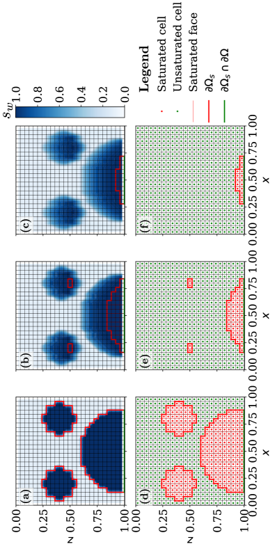
Figure 1: Gravity-dominated drainage of multiple saturated drops across an otherwise unsaturated ($s_{w}=10\%$) porous reservoir demonstrating the hyperbolic-elliptic PDE solution algorithm. The saturation contours are shown at dimensionless times $t^{\prime}=$ (a) 0, (b) 0.025 and (c) 0.05. Their corresponding dynamically evolving saturated and unsaturated cells as well as faces are respectively shown in subfigures (d), (e) and (f). The gravity aligns with $+z$ direction, i.e., $\hat{\textbf{g}}=(0,0,1)^{T}$. The unit square domain is divided uniformly into $25\times 25$ cells. Here the number of cells in $z$ and $x$ directions are $m=25$ and $n=25$ respectively and the total number of cells are $N=nm=25\times 25=625$. The number of faces with normals in $z$ direction are $N_{fz}=n(m+1)=25\times 26=650$ and in $x$ direction are $N_{fx}=(n+1)m=650$. The total number of cell faces are $N_{f}=N_{fx}+N_{fz}=1300$.

Algorithm 1 Hyperbolic-elliptic PDE solution algorithm

1:while $t<T$ do $\triangleright$ Time loop

2:     Calculate gravity dominated flux $\textbf{q}_{u}$ ($=\textbf{q}^{i}$) at all cell faces in $\Omega$

3:     Flag all the saturated cells $\Omega_{s}$ where $s_{w}>s_{w,T}$ (threshold saturation) $\triangleright$ $s_{w,T}\sim 1-s_{gr}$

4:     if $\Omega_{s}\neq\{\}$ then $\triangleright$ Saturated region flux evaluation loop

5:         Set Dirichlet boundary condition on head, $h=-\int_{\textbf{0}}^{\textbf{x}}\hat{\textbf{g}}\cdot\mathrm{d}\textbf{x}$, in unsaturated cells

6:         Set head, $h=-\int_{\textbf{0}}^{\textbf{x}}\hat{\textbf{g}}\cdot\mathrm{d}\textbf{x}$, in saturated cells on the domain boundary ($\partial\Omega_{s}\cap\partial\Omega$) to enable outflow

7:         Solve Laplace-type equation (16) implicitly for head $h$

8:         Calculate saturated region’s face fluxes at all cell faces in $\Omega_{s}$ using Darcy’s law, i.e., $\textbf{q}_{s}=-K\nabla h$

9:         Substitute the saturated cells’ face fluxes in $\textbf{q}^{i}$ considering the front motion criteria (19) on $\partial\Omega_{s}$

10:         $\triangleright$ Domain boundaries which are saturated ($\partial\Omega\cap\partial\Omega_{s}$) only utilize saturated flux unless a boundary condition is specified      

11:     end if

12:     Calculate the time step $\Delta t^{i}$ from equation (17)

13:     Update the saturation $s_{w}^{i+1}$ explicitly from Equation (18)

14:     Update time counter $t^{i+1}=t^{i}+\Delta t^{i}$

15:end while

4 Numerical tests

In this section we provide one and two dimensional, steady and transient test problems. We further validate our numerical solver against their corresponding analytical results. For the examples considered in this section the absolute permeability, $\mathrm{k}(\phi)$, and relative permeability of water, $k_{rw}(s_{w})$, follow power laws (Kozeny, 1927; Carman, 1937; Brooks and Corey, 1964) as

$$\mathrm{k}(\phi)=\mathrm{k}_{0}\phi^{\textrm{m}}\quad\text{ and }\quad k_{rw}(s_{w})=k_{rw}^{0}\left(\frac{s_{w}-s_{wr}}{1-s_{gr}-s_{wr}}\right)^{\textrm{n}},$$ (20)

where $\mathrm{k}_{0},k_{rw}^{0}$, m and n are model constants. Here the residual water and gas saturations are given by $s_{wr}$ and $s_{gr}$ respectively. The normalized relative permeability is $k_{r}(s_{w},\textrm{n})=k_{rw}/k_{rw}^{0}=\left(\frac{s_{w}-s_{wr}}{1-s_{gr}-s_{wr}}\right)^{\textrm{n}}$. The residual saturations are set to zero ($s_{wr}=s_{gr}=0$) in the numerical examples to match with the analytical results. Moreover, the power law exponents are set to $\textrm{m}=3$ and $\textrm{n}=2$ unless stated otherwise. The threshold for activation of the saturated region is $s_{w,T}=99.9\%$. The following dimensionless variables are introduced for depth, volumetric flux and time for sake of generality,

$$z^{\prime}=\frac{z}{z_{0}},\quad\textbf{q}^{\prime}=\frac{\textbf{q}}{K}\quad\text{and}\quad t^{\prime}=\frac{tK}{z_{0}},$$ (21)

where $z_{0}$ is the characteristic depth (m) and $K$ is the saturated hydraulic conductivity (m/s) given by $K=\rho_{w}g\mathrm{k}_{0}\phi_{0}^{\textrm{m}}k_{rw}^{0}/\mu_{w}$ with $\phi_{0}$ being the characteristic porosity of the problem. Typically, $\phi_{0}$ is the porosity at the surface ($z=0$) unless otherwise stated. For all the test cases presented in this section, the gravity vector, g, is aligned with the depth coordinate, $z$, such that the angle $\alpha=0$ and therefore $\hat{\textbf{g}}=(0,0,1)^{T}$.

4.1 One-dimensional test cases

4.1.1 Drainage from a saturated soil

The first case is a simple drainage of a fully-saturated soil with uniform porosity $\phi_{0}$. It corresponds to infiltration following halt of a heavy rainfall which saturates the soil. It leads to formation of a self-smoothening front called rarefaction wave (LeVeque, 1992). This simple problem can help verify that the model captures the fast-moving rarefaction wave and the transition of the domain from saturated to unsaturated. The solution to this problem can be derived from the theory of hyperbolic equations (LeVeque, 1992) as

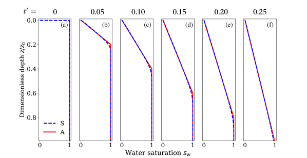
Figure 2: Drainage of an initially saturated, 50% porous reservoir at different dimensionless times. The blue lines show the simulation results and red lines show analytic results. The numerical grid is 400 uniform cells on a domain with unit depth.

$$s_{w}(z^{\prime},t^{\prime})=\begin{cases}s_{wr},\quad z^{\prime}=0\\ s_{wr}+\left(\frac{z^{\prime}\phi_{0}}{\textrm{n}t^{\prime}}(1-s_{gr}-s_{wr})^{\textrm{n}}\right)^{\frac{1}{\textrm{n}-1}},\quad 0<\frac{z^{\prime}}{t^{\prime}}<\lambda^{\prime}\\ (1-s_{gr}),\quad\frac{z^{\prime}}{t^{\prime}}\geq\lambda^{\prime}\end{cases}$$ (22)

where $\lambda^{\prime}=\frac{\lambda}{K}=\frac{\textrm{n}}{\phi_{0}(1-s_{gr}-s_{wr})}$ is the dimensionless characteristic speed for the saturated domain moving downwards. Please note that in the dimensional case, $q=Kk_{r}(s_{w},\textrm{n})$ and therefore, the exponent m does not appear in the dimensionless solution (22).

Figure 2a shows a 50% porous reservoir initially saturated completely, i.e., $s_{w}=1$. Drainage of an initially saturated porous reservoir leads to formation of rarefaction wave which travels in the direction of the gravity (see Figures 2b-2f). Here the saturation linearly varies inside the rarefaction wave as the relative permeability-saturation power law exponent is $\textrm{n}=2$. For this problem the surface does not require a boundary condition whereas the base is an outflow. The domain of unit depth is divided uniformly into 400 cells. The numerical solutions obtained from the present technique agree very well with the analytical results.

4.1.2 Infiltration in a two-layered soil

Next 1-D problem is more challenging which concerns transitional infiltration in a dry, two-layered soil leading to formation of self-sharpening wetting fronts known as shock waves (LeVeque, 1992) as well as a fully-saturated region. Consider a two-layered, low-textured soil with a jump at $z^{\prime}=1$ with porosities and permeabilities $\phi_{u},\mathrm{k}_{u}$ and $\phi_{l},\mathrm{k}_{l}$ in upper and lower layers respectively with $\phi_{u}>\phi_{l}$ and $\mathrm{k}_{u}>\mathrm{k}_{l}$. Therefore the saturated hydraulic conductivities in the upper and lower layer are $K_{u}$ ($=K$) and $K_{l}$ respectively. The soil is initially dry ($s_{w}(\textbf{x})=0$), as shown in Figure 3a.

When there is a transitional rainfall at a rainfall rate, $R$ ($K_{l}<R<K_{u}$), an unsaturated wetting front propagates downwards with constant velocity whose time-dependent location can be found using Rankine-Hugoniot jump condition (see Figure 3b) (LeVeque, 1992). Since the less porous layer is unable to accommodate the water flux as $K_{l}<R$, a fully saturated region forms at the location of the jump which expands normally outwards as shown in Figures 3c-3d. The initial wetting front thus bifurcates into two fronts moving upwards and downwards. Once the upward moving shock reaches the surface, ponding occurs (see Figures 3c-3d). The locations of all the fronts can be found analytically using extended kinematic-wave approximation, as given in Shadab and Hesse (2022).

The numerical experiments consider a dimensionless rainfall rate of $R/K_{u}=0.64$. The domain $z^{\prime}={z}/{z_{0}}\in[0,2]$ is uniformly divided into 400 cells with porosity jump at $z^{\prime}=1$. The porosity in upper region ($z^{\prime}<1$) is $\phi_{u}=0.5$ whereas porosity in the lower region ($z^{\prime}\geq 1$) is $\phi_{u}=0.2$. The numerical results agree well with the analytical results from Shadab and Hesse (2022). The lower boundary does not require a condition whereas the upper boundary is set to a constant saturation $s_{w}=0.8$ corresponding to $R/K_{u}=0.64$ which helps evade the numerical switching of the flux before and after ponding.

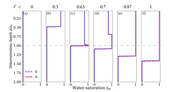
Figure 3: Infiltration process in an initially dry two-layered soil for $R/K_{u}=0.64$, $\phi_{u}=0.5$ and $\phi_{l}=0.2$ with jump at $z^{\prime}=1$ shown at different dimensionless times $t^{\prime}=$ (a) 0, (b) 0.3, (c) 0.63, (d) 0.7, (e) 0.87 and (f) 1. The blue lines show the numerical solution (denoted as S) and the red lines show the analytical solution (denoted as A) given in Shadab and Hesse (2022). The dashed grey line at $z^{\prime}=1$ ($z=z_{0}$) refers to the location of the jump.

4.2 Two-dimensional steady test cases

For the two-dimensional problems, the gravity is vertically downward direction, i.e., $\hat{\textbf{g}}\equiv(0,0,1)^{T}$. So the dimensionless horizontal direction variable, $x^{\prime}=x/z_{0}$, adds up to the set of dimensionless variables provided earlier in Equation (21).

4.2.1 Perched aquifer over a horizontal barrier

This test concerns an idealized two-dimensional plume which develops when a constant discharge per unit depth (in third dimension), $Q_{i}$, of water is injected into a reservoir which includes a horizontal flow barrier of characteristic length, $L$, much greater than its height (see Figure 4a). As the fluid falls due to gravity, it spreads laterally above the barriers. The impermeable barrier divides the incident discharge per unit width $Q_{i}$ into $Q_{a}$ and $Q_{b}$, which can be estimated using the Dupuit approximation (Bear, 1972; Huppert and Woods, 1995).

The fraction ($f_{b}$) of the incident discharge per unit width $Q_{i}$ which spills over the right end of the barrier at $x=L_{b}$, with $x=0$ being the location of the injector (see Figure 4a), is given by

$$f_{b}=\frac{Q_{b}}{Q_{a}+Q_{b}}=\frac{L_{a}}{L_{a}+L_{b}}$$ (23)

For the numerical experiments, a 40% porous domain $\Omega\equiv[0,7]\times[0,4]$ is divided into $140\times 80$ cells. The impermeable barrier is placed in the region $[0.5,6.5]\times[3,3.3]$ where no penetration boundary condition is imposed. A sufficiently thin fluid flux of dimensionless width 0.2 is injected at the top which results in an initial saturation of $s_{w}=97.5\%$. Boundary conditions are outflow at the bottom boundary and are not required elsewhere.

Here a nearly saturated fluid is injected into a porous domain which later saturates when fluid collects over the impermeable barrier. The fluid outflow at either side of the plate varies due to change in the horizontal location. The experiments from Hesse and Woods (2010), shown in Figures 4a-4d, illustrate this behavior which qualitatively matches with our numerical solutions, shown in Figures 4e-4h, corresponding to the same injector locations. Further, an excellent quantitative comparison between the theoretical, experimental and simulation results can be observed for the dependence of flux partitioning, $Q_{a}/(Q_{a}+Q_{b})$, on the injector location, $L_{a}/(L_{a}+L_{b})$, as shown in Figure 4i.

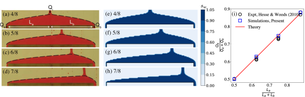
Figure 4: Flux partitioning in a steady gravity current passing over a barrier. The subcaptions represent the ratio of x-location of the injector with the plate length, with origin as the left end of the plate. (a-d): Experiment conducted by Hesse and Woods (2010) with glycerol in a Hele-Shaw cell of width 3 mm and a barrier of width 30 cm. (e-f): Simulations conducted using the algorithm proposed in the present work. (i) Dependence of the flux partitioning, $Q_{b}/(Q_{a}+Q_{b})$, on the effect length of the plate ends, $L_{a}/(L_{a}+L_{b})$.

4.2.2 Unconfined aquifer with a vertical seepage face

Free surface flow in homogeneous porous reservoirs is a crucial geophysical problem (Bear, 1972; Polubarinova-Kochina, 2015). For example, the steady unconfined groundwater aquifers which help design the hydraulic structures such as earth dams or river embankments (Simpson et al., 2003; Scudeler et al., 2017; Shadab et al., 2021). In this steady flow problem, fluid is injected at the left boundary which seeps across the reservoir and exits from the right face called the seepage face.

The domain $\Omega\equiv[0,1]\times[0,1]$ is divided into a uniform mesh of $75\times 75$ cells which is initially dry, i.e., $s_{w}(\textbf{x})=0~{}\forall\textbf{x}\in\Omega$. The medium is 50% porous although the effects of porosity are scaled out. The boundary conditions on the left is a fixed discharge per unit width (m${}^{\textrm{2}}$/s), $Q$, which is scaled as $Q/(KL)$ with the characteristic length, $z_{0}$, being the horizontal extent of the reservoir, $L$. The boundary condition at the seepage face on right is applied when a part of the boundary saturates by fixing the head to $h=-z$ on the corresponding boundary cells, similar to unsaturated cells. The rest of the boundaries are no-flow (natural).

The approximate analytical solution to this problem is provided by Polubarinova-Kochina (2015) for low aspect ratio reservoirs, i.e., when horizontal extent of the aquifer is close to its vertical extent. It is evaluated by free software given in Shadab et al. . The numerical results for free surface height are very close to the analytical solution for $Q/(KL)=0.087$ and $0.211$ as shown in Figures 5a and 5b respectively. Moreover, the variation in the dimensionless height of seepage face, $H_{0}/L$, with the dimensionless discharge per unit width, $Q/KL$, is given in Figure 5c which shows an excellent quantitative agreement in between the analytical and the numerical results.

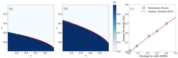
Figure 5: Steady unconfined aquifer with a vertical seepage face for dimensionless discharge per unit widths, $Q/(KL)=$ (a) 0.087 and (b) 0.211. (c) Variation of dimensionless seepage face heights, $H_{0}/L$, with the dimensionless discharge per unit width. The red lines are Polubarinova-Kochina (2015) analytic solutions evaluated from the software given in Shadab et al. .

4.3 Two-dimensional transient test cases

4.3.1 Fluid drainage from the edge of a porous reservoir

The first transient test is on buoyancy driven drainage from the edge of a porous reservoir (Zheng et al., 2013). This phenomenon occurs in a large variety of industrial and geophysical processes (Zheng et al., 2013). Consider a rectangular, homogeneous reservoir which is fully saturated initially. If all boundaries are no-flow except the right boundary ($x=L$) which is an outflow, the system results in a self-similar gravity current which follows nonlinear diffusion equation. The self-similar analysis neglects the effects of seepage face and vertical flow which is a good approximation if the aquifer is low aspect ratio where the horizontal extent of the aquifer is much larger than its vertical extent. The approximate analytic solution of the free-surface height, $h(x,t)$, is described using dimensionless variable defined as

$$\quad h^{\prime}=\frac{h}{z_{0}}.$$ (24)

We pick the characteristic length, $z_{0}$, to be the length of the reservoir, $L$. In this case the dimensionless solution can be expressed as

$$h^{\prime}=\frac{\mathrm{f}(\eta)\phi}{t^{\prime}}$$ (25)

where the dimensionless function $\textrm{f}(\eta)$, which depends on $\eta=x/L$, is defined by the boundary value problem

$$\frac{\mathrm{d}}{\mathrm{d}\eta}\left(\mathrm{f}\frac{\mathrm{d}\mathrm{f}}{\mathrm{d}\eta}\right)+\mathrm{f}=0,\quad\text{subject to}\quad\frac{\mathrm{d}\mathrm{f}}{\mathrm{d}\eta}\bigg{|}_{0}=0\quad\text{and}\quad\mathrm{f}(1)=0.$$ (26)

Moreover, the total volume of fluid inside the domain at a later time is defined as $\mathcal{V}(t)=w\int_{0}^{L}h(x,t)\mathrm{d}x$ where $w$ is the depth in the third dimension. So the total dimensionless volume of fluid inside the domain at any time is $\mathcal{V}^{\prime}(t^{\prime})$ which is defined as

$$\mathcal{V}^{\prime}(t^{\prime})=\frac{\mathcal{V}(t)}{wL^{2}}=\frac{\phi}{t^{\prime}}\int_{0}^{1}\mathrm{f}(\eta)\mathrm{d}\eta\propto\frac{1}{t^{\prime}}.$$ (27)

where $\mathcal{V}^{\prime}=\frac{\mathcal{V}(t)}{wz_{0}^{2}}$ and $z_{0}=L$.

For the numerical simulation, a low aspect ratio domain $\Omega\equiv[0,3]\times[0,1]$ is considered to reduce the effect of vertical flow and the height of seepage face. The domain is divided into $150\times 100$ cells. Although the reservoir considered is $50\%$ porous, the effects of porosity are scaled out. The medium is $90\%$ saturated initially however the initial condition does not affect the solution at late stages. All boundaries are no flow except the right one which is an outflow. The resulting gravity current diffuses out from the edge of the reservoir as shown in Figures 6a-6e. Initially, from time $t^{\prime}=0$ (not shown here) to approximately $t^{\prime}=6$ (see Figure 6a), the analytic solution catches up to the numerical solution due to the effect of the initial condition. At late stages they agree fairly well with each other but numerically computed free surface heights are slightly higher than the analytical results. The difference in the results may arise due to non-zero vertical flow effects as well as finite seepage face height which affects the free surface height inside the domain. This difference is also transcended to the evolution of dimensionless volume shown in Figure 6f, where at late stages the simulated volume of fluid is more than the analytical volume evaluated from (27). But the numerical result follows the theoretical scaling, $\mathcal{V}^{\prime}\sim t^{\prime-1}$.

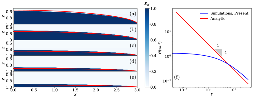
Figure 6: Drainage from the edge of a porous reservoir at dimensionless times $t^{\prime}=$ (a) $6$, (b) $12$, (c) $18$, (d) $24$ and (e) $30$. (f) The corresponding evolution of total dimensionless volume of fluid inside the domain, $\mathcal{V}/(wL^{2})$. In all plots, the red lines show the analytic solutions. The blue lines or contours show numerical solution.

4.3.2 Propagation of a gravity current into a porous layer

The problem of gravity currents exists in context of subsurface groundwater flows (Huppert and Woods, 1995). Consider the instantaneous release of finite volume of fluid, $\mathcal{V}$ (m${}^{\text{3}}$), in a horizontal porous medium with constant porosity $\phi_{0}$. It results in a self-similar gravity current which follows a nonlinear diffusion equation in the limit of small aspect ratio (Huppert and Woods, 1995). The approximate analytic solution of the free-surface height, $h(x,t)$, is described using dimensionless variables introduced in section 4.3.1. The dimensionless analytical solution is therefore given by

$$h^{\prime}(x^{\prime},t^{\prime})=\left(\frac{\phi_{0}\mathcal{V}^{\prime 2}}{t^{\prime}}\right)^{\frac{1}{3}}f(\omega),\quad\text{with }f(\omega)=\frac{\omega_{0}^{2}-\omega^{2}}{6},\quad 0<\omega<\omega_{0}$$ (28)

where $\omega_{0}=\left(\frac{9}{\phi_{0}}\right)^{1/3}$, $\omega=\frac{x^{\prime}}{\left(\mathcal{V}^{\prime}t^{\prime}/\phi_{0}\right)^{1/3}}$ and $\mathcal{V}^{\prime}=\mathcal{V}/wz_{0}^{2}$, as introduced in Section 4.3.1.

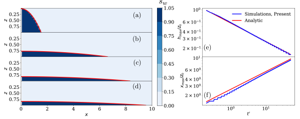
Figure 7: Gravity current propagation on a horizontal porous layer at dimensionless times $t^{\prime}=$ (a) 0.2, (b) 16, (c) 32 and (d) 48. The spatial coordinates are dimensionless. The blue contour shows the solution from the proposed numerical method. The corresponding evolution of (e) dimensionless maximum height of the mound and its (f) dimensionless maximum spreading distance along x-axis is also provided. The solid blue line refers to the numerical solution. In all the plots, the red line shows the approximate analytic solution given by Equation (28).

The 50% porous domain $\Omega\equiv[0,25]\times[0,1]$ is divided into $200\times 100$ cells. In this problem, the initial condition is set as the analytic solution at $t^{\prime}=0.2$ (see Figure 7a). The boundary conditions are natural on left and bottom boundaries and are not required on top and right boundaries. The gravity current thus generated diffuses towards right as shown in Figures 7b-7d. The numerical solutions are at par with the approximate analytical results given by Equation (28) shown by red lines. It can be quantitatively observed in the time evolution of maximum height of the mound, $h^{\prime}_{max}$, along $z$ axis and maximum spreading distance, $x^{\prime}_{max}$, along the $x$ axis in Figures 7e and 7f respectively. Although both numerical results quite nicely follow the analytical results with the theoretical scaling ($h^{\prime}_{max}\sim t^{\prime-1/3}$, $x^{\prime}_{max}\sim t^{\prime 1/3}$), there is a slight difference in the $x^{\prime}_{max}$ results due to finite spatial resolution.

4.3.3 Infiltration into a heterogeneous soil

Subsurface is very heterogeneous at multiple scales with a large scale, ordered layering (Zhu and Zhang, 2013). However, other heterogeneity is largely random in nature. Although both heterogeneities are crucial, the random one introduces uncertainty even when the large scale pattern is known. Consider a stationary random field which exhibits a constant distribution function for the parameter of interest (say permeability and/or porosity). Here the spatial correlation is only a function of the separation distance, and not of position within the random field. Soils exhibit a transverse anisotropy (see Zhu and Zhang (2013) for a review) where the horizontal scale of parameter fluctuation is often more than an order of magnitude larger than the vertical scale of fluctuation due to the nature of soil deposition (Yang et al., 2022). For example, Phoon and Kulhawy (1999) reports that the horizontal scale of fluctuation ($\theta_{x}$) is approximately 50 and 150 times larger than the vertical scale ($\theta_{z}$) for sand and clay soils respectively. As a result, the soil permeability (and/or porosity) varies more rapidly in the vertical direction and more smoothly along the horizontal direction. Assuming the scale of formation of fluctuation is elliptical, the exponential correlation function, $\mathcal{\varrho}$, for transverse anisotropy is given in Zhu and Zhang (2013) as

$$\varrho=\exp\left(-2\sqrt{\frac{\Delta\mathcal{X}^{2}}{\theta_{x}^{2}}+\frac{\Delta\mathcal{Z}^{2}}{\theta_{z}^{2}}}\right)$$ (29)

where $\Delta\mathcal{X}$ and $\Delta\mathcal{Z}$ are respectively the horizontal and vertical separation distances between two observations in the space. The symbols $\theta_{x}$ and $\theta_{z}$ denote the principal scales of fluctuation in the $x$ and $z$ directions respectively.

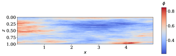
Figure 8: Porosity field of a stratified, heterogeneous soil with mean porosity $\phi_{mean}=46.5\%$, maximum porosity $\phi_{max}=85\%$ and minimum porosity $\phi_{min}=21.6\%$ with fluctuation lengths $\theta_{x}=10$ and $\theta_{z}=1$.

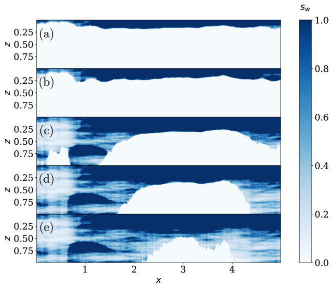
Figure 9: Time sequenced images of infiltration in a stratified, heterogeneous soil at dimensionless times $t^{\prime}=$ (a) 5, (b) 10, (c) 50, (d) 100 and (e) 250.

The matrix decomposition method is utilized in this approach which requires the defining a discrete set of $N$ spatial points at which the random field is sampled. Subsequently, it helps construct an $N$ by $N$ covariance matrix, C which quantifies the correlation between all of the spatial points being sampled. The exponential correlation function $\varrho$ (29) helps define the covariance matrix. For generating realizations of correlated random field, matrix decomposition method is often utilized (Zhu and Zhang, 2013). An expensive but exact method is Cholesky factorization (Trefethen and Bau III, 1997) which is performed on the covariance matrix to obtain upper ($\textit{{L}}^{T}$) and lower (L) triangular matrices as

$$\textit{{L}}~{}\textit{{L}}^{T}=\textit{{C}}.$$

Next an $N$ by $1$ vector X consisting of uncorrelated random numbers from a unit normal distribution is created. Then the corresponding $N$ by $1$ vector of correlated random variables, Y, is evaluated by computing LX and subsequently adding the mean, $\boldsymbol{\mu}$ as

$$\textit{{Y}}=\textit{{L~{}X}}+\boldsymbol{\mu}$$ (30)

Since the permeability has order of magnitude variations in a soil, the final transformation, $\textbf{k}=10^{\textit{{Y}}}$, yields the $N\times 1$ vector of absolute permeability inside each cell.

This test involves a stratified, heterogenous soil with two fluctuation lengths, $\theta_{z}=1$ and $\theta_{x}=10$ with the mean dimensionless permeability, $\mathrm{k}_{mean}/\mathrm{k}_{0}=1$. Then the porosity field, $\phi(\textbf{x})$, is evaluated by using maximum value of porosity, $\phi_{max}$ ($\phi_{max}$=85$\%$ in the present problem), and the maximum evaluated dimensionless permeability, $\mathrm{k}_{max}/\mathrm{k}_{0}$, from Equation (20) as $\phi(\textbf{x})=\phi_{max}\left(\mathrm{k}(\textbf{x})/\mathrm{k}_{max}\right)^{1/\textrm{m}}$. Choosing a higher value of m ($\textrm{m}=8$) helps fix the mean porosity to $46.5\%$ and minimum to $21.6\%$ which are the close to the values for the fine sand (Das and Das, 2008). The resulting heterogeneous porosity profile is shown in Figure 8. This problem concerns rainwater infiltration in a layered soil in a domain $\Omega\equiv[0,5]\times[0,1]$ which is divided into $250\times 100$ cells. The entire surface boundary condition ($z^{\prime}=0$) is of complete saturation ($s_{w}=1$), which corresponds to a heavy rainfall, in order to visualize the effects of multidimensional flow. The rest of the boundaries are outflows.

The resulting gravity driven infiltration is shown in Figure 9 at different dimensionless times. Initially, an almost uniform front moves downwards (see Figures 9a-9b). But since the soil is more porous on the left half than the right half, the latter leads to formation of fully saturated region as shown in Figures 9c-9d. Whereas the front in the left half infiltrates faster. The water saturation on the left is lower in general as the medium is more porous as shown in Figure 9e. Due to presence of lower porosity layer on the right half, the soil layers beneath remain inaccessible for very long periods of time. Inside the fully saturated regions, the dynamics switches from gravity driven flow to pressure driven flow. Once a saturated region forms, the flow can move in directions other than the gravity vector, i.e., laterally or upwards leading to ponding and runoff. In this problem multiple saturated (perched) regions form inside the domain but they are taken care of simultaneously and efficiently in the present approach. This is a challenging problem due to soil heterogeneity as well as formation of multiple saturated regions.

5 Conclusions

In this paper we first introduced a hyperbolic-elliptic partial differential equation based model for variably saturated groundwater flow in the limit of negligible capillary forces. Then we proposed a simple, efficient and conservative numerical method to simulate such flow. The technique takes care of the degeneracy in the complete-saturation limit by considering the full-two phase flow physics which leads to an elliptic problem in the saturated regions. The developed multidimensional numerical model is based on conservative finite difference scheme and tensor-product grid approach which can efficiently and robustly handle sharp saturation gradients as well as fully saturated regions. This physics-based variably saturated flow model can be straightforwardly extended to include capillary effects. Next, we provide a suite of challenging benchmark problems in one- and two-dimensions along with their corresponding analytical results. These problems involve variably saturated flow which can help in verification and validation (V&V) as well as performance comparison of numerical solvers. Our simulation results show excellent agreement with the analytical solutions for all the proposed problems. Finally we consider a complicated test of rainwater infiltration inside a stratified, heterogeneous soil. This test illustrates an intricate infiltration dynamics which involves formation and evolution of multiple saturated regions also causing perching and lateral flow.

Appendix A One dimensional operators

The gradient, divergence and mean operators are approximated with a second-order finite difference approximation. For a one-dimensional grid with $n$ ($m$ ; $l$) cells of uniform width $\Delta x$ ($\Delta z$ ; $\Delta y$) and therefore $(n+1)$ faces, the $n$ by $(n+1)$ discrete divergence operator, $\textbf{D}_{n}:\mathbb{R}^{n+1}\to\mathbb{R}^{n}$, and the $(n+1)$ by $n$ discrete gradient operator, $\textbf{G}_{n}:\mathbb{R}^{n}\to\mathbb{R}^{n+1}$, respectively take the forms

$$\nabla\cdot\approx\textbf{D}_{n}=\frac{1}{\Delta x}\begin{bmatrix}-1&1&&&&\\ &-1&1&&&\\ &&\ddots&\ddots&&\\ &&&-1&1&\\ &&&&-1&1\end{bmatrix}_{n~{}\times~{}(n+1)}\text{and}\quad\nabla\approx\textbf{G}_{n}=\frac{1}{\Delta x}\begin{bmatrix}0&&&&&\\ -1&1&&&&\\ &-1&1&&&\\ &&\ddots&\ddots&&\\ &&&-1&1&\\ &&&&-1&1\\ &&&&&0\end{bmatrix}_{(n+1)~{}\times~{}n}.$$ (31)

Here the symbols $\mathbb{R}^{n}$ and $\mathbb{R}^{n+1}$ refer to the vector spaces of the cell centers and cell faces respectively. The discrete gradient, $\textbf{G}_{n}$, assumes a natural boundary condition, i.e., no flow across the domain boundary. In a similar fashion, the $(n+1)$ by $n$ algebraic mean operator, $\textbf{M}_{n}:\mathbb{R}^{n}\to\mathbb{R}^{n+1}$, can be constructed as

$$\textbf{M}_{n}=\frac{1}{2}\begin{bmatrix}m_{b}&&&&&\\ 1&1&&&&\\ &1&1&&&\\ &&\ddots&\ddots&&\\ &&&1&1&\\ &&&&1&1\\ &&&&&m_{b}\end{bmatrix}_{(n+1)~{}\times~{}n}.$$ (32)

Here $m_{b}=2$ for placing the cell value at the boundary face without interpolating and $m_{b}=0$ for a zero value (no-flow boundary condition) as placeholders. The entries corresponding to the boundaries are typically replaced by the boundary conditions which will be discussed in Appendix C.

Advection operator. For solving the hyperbolic Richards equation, the advective flux computation requires value of saturation (or soil moisture content) at the faces to evaluate the hydraulic conductivity. For that purpose, we use Darcy flux-based upwinding to compute the face values of saturation (Godunov and Bohachevsky, 1959). In matrix form, we construct an advection matrix operator, $\textbf{A}(\textbf{q}):\mathbb{R}^{n}\to\mathbb{R}^{n+1}$, which takes in the $(n+1)$ face flux vector $\textbf{q}=[q_{1},q_{2},\ldots,q_{n-1},q_{n+1}]^{T}$ and provides the $(n+1)$ by $n$ advection operator A. The advection operator A is constructed as

$$\textbf{A}_{n}=\textbf{Q}_{(n+1)}^{+}\textbf{A}_{n}^{+}~{}+~{}\textbf{Q}_{(n+1)}^{-}\textbf{A}_{n}^{-}$$ (33)

where in one-dimension,

$$\textbf{Q}_{(n+1)}^{+} =\begin{bmatrix}q_{1}^{+}&&&&&\\ &q_{2}^{+}&&&&\\ &&q_{3}^{+}&&&\\ &&&\ddots&&\\ &&&&q_{n}^{+}&\\ &&&&&q_{n+1}^{+}\\ \end{bmatrix}_{(n+1)~{}\times~{}(n+1)},\quad \textbf{Q}_{(n+1)}^{-}=\begin{bmatrix}q_{1}^{-}&&&&&\\ &q_{2}^{-}&&&&\\ &&q_{3}^{-}&&&\\ &&&\ddots&&\\ &&&&q_{n}^{-}&\\ &&&&&q_{n+1}^{-}\\ \end{bmatrix}_{(n+1)~{}\times~{}(n+1)},$$ (34)

$$\textbf{A}_{n}^{+} =\begin{bmatrix}0&&&&&\\ 1&&&&&\\ &1&&&&\\ &&\ddots&&&\\ &&&1&&\\ &&&&1&\\ &&&&&1\end{bmatrix}_{(n+1)~{}\times~{}n}\quad\quad\quad\text{and}\quad \textbf{A}_{n}^{-}=\begin{bmatrix}1&&&&&\\ &1&&&&\\ &&1&&&\\ &&&\ddots&&\\ &&&&1&\\ &&&&&1\\ &&&&&0\end{bmatrix}_{(n+1)~{}\times~{}n},$$ (35)

where $q_{i}^{-}$ refers to negative flux, $\min\{q_{i},0\}$, and $q_{i}^{+}$ refers to positive flux, $\max\{q_{i},0\}$, for $i\in\{1,2,\ldots,n,n+1\}$.

Appendix B Discrete operators in three dimensions

The present framework can be easily extended to three dimensions with the same approach. The tensor product grid enables a straightforward extension from two to three dimensions with a few more lines of code. In three-dimensions, we use a regular Cartesian mesh with $n$ cells of size $\Delta x$ in $x$ direction, $m$ cells of size $\Delta y$ in $y$ direction and $l$ cells of size $\Delta z$ in $z$ direction. The three dimensional divergence, gradient and mean operators are then composed of three block matrices as

$$\textbf{H}=\begin{bmatrix}\textbf{H}_{x}\\ \textbf{H}_{y}\\ \textbf{H}_{z}\end{bmatrix},\quad\textbf{H}\in\{\textbf{D}^{T}~{},~{}\textbf{G}~{},~{}\textbf{M}\}$$ (36)

with directional operators defined as

$$\textbf{H}_{x}=\textbf{I}_{l}\otimes(\textbf{H}_{n}\otimes\textbf{I}_{m}),\quad \quad\textbf{H}_{y}=\textbf{I}_{l}\otimes(\textbf{I}_{n}\otimes\textbf{H}_{m})\quad\text{and}\quad\textbf{H}_{z}=\textbf{H}_{l}\otimes(\textbf{I}_{n}\otimes\textbf{I}_{m}),\quad\textbf{H}\in\{\textbf{D}~{},~{}\textbf{G}~{},~{}\textbf{M}\}.$$ (37)

Similar to two dimensional operators given in Section 3.1 the one dimensional operators, $\{\textbf{D}_{\alpha},\textbf{G}_{\alpha},\textbf{M}_{\alpha}\}$ for $\alpha\in\{n,m,l\}$, can be evaluated from Equations (31-32). Moreover, the $N_{f}$ by $N$ advection operator A can be expressed in three dimensions as

$$\textbf{A}=\textbf{Q}^{+}\textbf{A}^{+}~{}+~{}\textbf{Q}^{-}\textbf{A}^{-},$$ (38)

where $N_{f}$ is the total number of faces which is the summation of $x$, $y$ and $z$ normal faces, i.e., $N_{f}=N_{fx}+N_{fy}+N_{fz}$ and $N$ is total number of cells given by $N=nml$. Additionally, the three-dimensional block matrix of positive or negative fluxes, $\textbf{Q}^{\pm}$, and the advection operator, $\textbf{A}^{\pm}$, are given by

$$\textbf{Q}^{\pm}=\begin{bmatrix}\textbf{Q}_{x}^{\pm}&&\\ &\textbf{Q}_{y}^{\pm}&\\ &&\textbf{Q}_{z}^{\pm}\end{bmatrix}_{N_{f}~{}\times~{}N_{f}}\quad\text{and}\quad \textbf{A}^{\pm}=\begin{bmatrix}\textbf{A}_{x}^{\pm}\\ \textbf{A}_{y}^{\pm}\\ \textbf{A}_{z}^{\pm}\end{bmatrix}.$$ (39)

In three-dimensions, the number of $x$, $y$ and $z$ normal faces are $N_{fx}=(n+1)ml$, $N_{fy}=n(m+1)l$ and $N_{fy}=nm(l+1)$ respectively. $\textbf{Q}_{x}^{\pm}$ ($\textbf{Q}_{y}^{\pm}$ ; $\textbf{Q}_{z}^{\pm}$) is the $N_{fx}$ by $N_{fx}$ ($N_{fy}$ by $N_{fy}$ ; $N_{fz}$ by $N_{fz}$) diagonal matrix with $x$ ($y$ ; $z$) positive/negative face Darcy fluxes in the diagonal. Moreover, the $x$, $y$ and $z$ matrix components of $\textbf{A}^{+}$ and $\textbf{A}^{-}$ are expressed similar to the 3D discrete operators (37) as follows,

$$\textbf{A}_{x}^{\pm}=\textbf{I}_{l}\otimes\left(\textbf{A}_{n}^{\pm}\otimes\textbf{I}_{m}\right),\quad\quad\textbf{A}_{y}^{\pm}=\textbf{I}_{l}\otimes\left(\textbf{I}_{n}\otimes\textbf{A}_{m}^{\pm}\right) \quad\text{and}\quad\textbf{A}_{z}^{\pm}=\textbf{A}_{l}^{\pm}\otimes\left(\textbf{I}_{n}\otimes\textbf{I}_{m}\right)$$ (40)

where $\textbf{A}_{n}^{\pm}$, $\textbf{A}_{m}^{\pm}$ and $\textbf{A}_{l}^{\pm}$ are again the one-dimensional operators as expressed in (34). For the definitions of one dimensional operators, see Equations (31-32). The sequence is chosen to respect the internal ordering of Matlab where the cells and faces are ordered in $y$ direction first, then $x$ and then $z$. Please note that the vertical dimension in this case $y$ instead of $z$ as proposed earlier in two-dimensional cases for sake of consistency with the literature.

Appendix C Boundary conditions

Boundary conditions are required so that the PDE problem becomes well posed. In this section, we discuss the implementation of the boundary conditions taking the discrete system (16) as an example. However, its application is more general and which is also in the saturation equation (18). Natural boundary conditions (zero gradient/no flux) are implemented in the discrete gradient operator so there is no extra effort for no flow boundary conditions. However, if gradient is not being used in the evaluation of the advective flux, the natural boundary condition is enforced in divergence operator by calculating it from $\textbf{D}=-\textbf{G}^{T}$ and/or the mean operator with $m_{b}=0$.

Neumann boundary condition. Its implementation is fairly straightforward. For zero flux at the boundary, nothing needs to be done since it is in-built in the discrete gradient. Although, the non-zero fluxes at the boundary are converted to an additional source term corresponding to Neumann boundary cells

$$f_{n}=q_{b}\frac{A}{V}$$ (41)

where $f_{n}$ is the source term from Neumann BC, $q_{b}$ is the boundary flux, $A$ is the area of the corresponding boundary face and $V$ is the volume of the same boundary cell. The extra source term for Neumann boundary takes the form of $N$ by $1$ vector, $\textbf{f}_{n}$, which is added to the governing discrete equation. For example, the governing discrete equation (16) becomes $\textbf{L}~{}\textbf{h}=\textbf{f}_{s}+\textbf{f}_{n}$.

Dirichlet boundary conditions. Since Dirichlet boundary conditions prescribe the unknowns (for example, head $h$) at the boundary cell centers, the numbers of unknowns thus have to be reduced in accordance with the constraints. The two cases are considered as follows:

a. Homogeneous Dirichlet BC: In this case, the system of equations has to be reduced according to the constraints. The idea is to project the original space $\mathbb{R}^{N}$ onto a reduced subspace $\mathbb{R}^{(N-N_{c})}$ using an orthogonal projection, eliminating the $N_{c}$ number of constraints (Trefethen and Bau III, 1997). The subspace of the reduced unknowns is the null space of the $N_{c}$ by $N$ constraint matrix B, i.e., $\mathcal{N}(\textbf{B})\in\mathbb{R}^{N-N_{c}}$, where B is defined as $\textbf{B}~{}\textbf{h}=\textbf{0}$. Any set of orthonormal basis for $\mathcal{N}(\textbf{B})$ can project the unknowns from full space $\mathbb{R}^{N}$ to the reduced space $\mathcal{N}(\textbf{B})\in\mathbb{R}^{(N-N_{c})}$. Therefore, an $N$ by $(N-Nc)$ projection matrix N can be constructed trivially with standard orthonormal bases. From an identity matrix $\textbf{I}_{N}$, B and N can be easily constructed by eliminating the columns for the former and keeping the rows for the latter, corresponding to the degree of freedom of the constraints. Here, $\textbf{N}^{T}\textbf{L}\hskip 2.84526pt\textbf{N}=\textbf{L}_{r}$ is the discrete linear operator $(N-N_{c})\times(N-N_{c})$ matrix in the bases of reduced subspace, $\textbf{h}_{r}=\textbf{N}^{T}\hskip 2.84526pt\textbf{h}$ is the $(N-N_{c})$ by $1$ vector of unknowns in the reduced subspace $\mathbb{R}^{(N-N_{c})}$ and $\textbf{f}_{s,r}=\textbf{N}^{T}\hskip 2.84526pt\textbf{f}_{s}$ is the $(N-N_{c})$ by $1$ vector of the source term in the reduced subspace $\mathbb{R}^{(N-N_{c})}$. The final reduced matrix equation is $\textbf{L}_{r}\textbf{h}_{r}=\textbf{f}_{s,r}$ which can be solved directly for $\textbf{h}_{r}$.

b. Heterogeneous Dirichlet BC: Dealing with non-zero Dirichlet boundary conditions is slightly more sophisticated. Using the (quasi-)linearity of the problem helps splitting the solution h into homogeneous $\textbf{h}_{0}$ and particular $\textbf{h}_{p}$ solution vectors of size $N$ by $1$ for solving the boundary value problem (Greenberg, 2013). The $N_{c}$ by $N$ constraint matrix B is the same as earlier which governs $\textbf{B}~{}\textbf{h}_{p}=\textbf{c}$ where c is the $N_{c}$ by $1$ vector of known boundary conditions.

$$\left.\begin{aligned} \textbf{B}\hskip 5.69054pt\textbf{h}_{0}=\textbf{0}\\ \textbf{B}\hskip 5.69054pt\textbf{h}_{p}=\textbf{c}\end{aligned}\right\}\hskip 5.69054pt\textbf{B}\hskip 2.84526pt(\textbf{h}_{0}+\textbf{h}_{p})=\textbf{c}$$ (42)

Since B right invertible matrix, $\textbf{B}\hskip 2.84526pt\textbf{B}^{T}$ is used which is $N_{c}\times N_{c}$ full rank matrix. We define the particular solution $\textbf{h}_{p,r}$ in reduced space $\mathbb{R}^{N_{c}}$ to be $\textbf{h}_{p,r}=\textbf{B}~{}\textbf{h}_{p}=\textbf{c}$ and $\textbf{h}_{p}=\textbf{B}^{T}~{}\textbf{h}_{p,r}$. Therefore, we solve $\textbf{B}^{T}~{}\textbf{B}~{}\textbf{h}_{p,r}=\textbf{c}$ to get $\textbf{h}_{p}$ from the Dirichlet boundary constraint matrix, B, and the Dirichlet boundary condition values, c.

Next, to find the homogeneous solution $\textbf{h}_{0}$, plugging the decomposed solution (42) in the discrete governing equation (16) gives the final system, $\textbf{L}~{}\textbf{h}_{0}=\textbf{f}_{s}+\textbf{f}_{D}$, where $\textbf{f}_{D}$ is source term from heterogeneous Dirichlet BCs, $\textbf{f}_{D}=-\textbf{L}~{}\textbf{h}_{p}$. Then similar to the homogeneous Dirichlet boundary condition case, the constraints are eliminated using orthogonal projection, again leading to a well-posed, reduced system of equations which can be solved for the homogeneous solution $\textbf{h}_{0}$. Finally, the solution can be evaluated from $\textbf{h}=\textbf{h}_{0}+\textbf{h}_{p}$.

References

- Bear (1972) Bear, J., 1972. Dynamics of Fluids in Porous Media. Dover, New York.
- Blunt (2017) Blunt, M., 2017. Multiphase Flow in Permeable Media. Cambridge University Press, Cambridge. doi:10.1017/9781316145098.
- Brooks and Corey (1964) Brooks, R., Corey, T., 1964. Hydrau uc properties of porous media. Hydrology Papers, Colorado State University 24, 37.
- Brustkern and Morel-Seytoux (1970) Brustkern, R.L., Morel-Seytoux, H.J., 1970. Analytical treatment of two-phase infiltration. Journal of the Hydraulics Division 96, 2535–2548.
- Carman (1937) Carman, P.C., 1937. Fluid flow through granular beds. Trans. Inst. Chem. Eng. 15, 150–166.
- Charbeneau (1984) Charbeneau, R., 1984. Kinematic Models for Soil Moisture and Solute Transport. Technical Report 6.
- Clapp and Hornberger (1978) Clapp, R., Hornberger, G., 1978. Empirical equations for some soil hydraulic properties. Water Resources Research 14, 601–604. URL: http://doi.wiley.com/10.1029/WR014i004p00601, doi:10.1029/WR014i004p00601.
- Colbeck (1972) Colbeck, S.C., 1972. A Theory of Water Percolation in Snow. Journal of Glaciology 11, 369–385. URL: https://www.cambridge.org/core/product/identifier/S0022143000022346/type/journal_article, doi:10.3189/S0022143000022346.
- Dai et al. (2019) Dai, Y., Zhang, S., Yuan, H., Wei, N., 2019. Modeling variably saturated flow in stratified soils with explicit tracking of wetting front and water table locations. Water Resources Research 55, 7939–7963.
- Das and Das (2008) Das, B.M., Das, B., 2008. Advanced soil mechanics. volume 270. Taylor & Francis New York.
- Farthing and Ogden (2017) Farthing, M.W., Ogden, F.L., 2017. Numerical Solution of Richards’ Equation: A Review of Advances and Challenges. Soil Science Society of America Journal 0, 0. URL: https://dl.sciencesocieties.org/publications/sssaj/abstracts/0/0/sssaj2017.02.0058, doi:10.2136/sssaj2017.02.0058.
- van Genuchten (1980) van Genuchten, M., 1980. A Closed-form Equation for Predicting the Hydraulic Conductivity of Unsaturated Soils1. Soil Science Society of America Journal 44, 892. doi:10.2136/sssaj1980.03615995004400050002x.
- Godunov and Bohachevsky (1959) Godunov, S., Bohachevsky, I., 1959. Finite difference method for numerical computation of discontinuous solutions of the equations of fluid dynamics. Matematičeskij sbornik 47, 271–306.
- Greenberg (2013) Greenberg, M.D., 2013. Foundations of applied mathematics. Courier Corporation.
- Hesse and Woods (2010) Hesse, M., Woods, A., 2010. Buoyant dispersal of CO2 during geological storage. Geophysical Research Letters 37, n/a–n/a. URL: http://doi.wiley.com/10.1029/2009GL041128, doi:10.1029/2009GL041128.
- Hoffman and Frankel (2018) Hoffman, J.D., Frankel, S., 2018. Numerical methods for engineers and scientists. CRC press.
- Huppert and Woods (1995) Huppert, H.E., Woods, A.W., 1995. Gravity-driven flows in porous layers. Journal of Fluid Mechanics 292, 55–69. URL: https://www.cambridge.org/core/product/identifier/S0022112095001431/type/journal_article, doi:10.1017/S0022112095001431.
- Kees (2004) Kees, C.E., 2004. Speed of propagation for some models of two-phase flow in porous media. Technical Report. North Carolina State University. Center for Research in Scientific Computation.
- Kollet et al. (2017) Kollet, S., Sulis, M., Maxwell, R.M., Paniconi, C., Putti, M., Bertoldi, G., Coon, E.T., Cordano, E., Endrizzi, S., Kikinzon, E., et al., 2017. The integrated hydrologic model intercomparison project, ih-mip2: A second set of benchmark results to diagnose integrated hydrology and feedbacks. Water Resources Research 53, 867–890.
- Kozeny (1927) Kozeny, J., 1927. Uber kapillare leitung der wasser in boden. Royal Academy of Science, Vienna, Proc. Class I 136, 271–306.
- Lax and Liu (1998) Lax, P.D., Liu, X.D., 1998. Solution of two-dimensional riemann problems of gas dynamics by positive schemes. SIAM Journal on Scientific Computing 19, 319–340.
- LeVeque (1992) LeVeque, R., 1992. Numerical Methods for Conservation Laws. Birkhaeuser Verlag.
- Leverett (1941) Leverett, M., 1941. Capillary Behavior in Porous Solids. Transactions of the AIME 142, 152–169. URL: http://www.onepetro.org/doi/10.2118/941152-G, doi:10.2118/941152-G.
- List and Radu (2016) List, F., Radu, F.A., 2016. A study on iterative methods for solving richards’ equation. Computational Geosciences 20, 341–353.
- Meyer and Hewitt (2017) Meyer, C., Hewitt, I., 2017. A continuum model for meltwater flow through compacting snow. Cryosphere 11, 2799–2813. doi:10.5194/tc-11-2799-2017.
- Miller et al. (2013) Miller, C.T., Dawson, C.N., Farthing, M.W., Hou, T.Y., Huang, J., Kees, C.E., Kelley, C., Langtangen, H.P., 2013. Numerical simulation of water resources problems: Models, methods, and trends. Advances in Water Resources 51, 405–437.
- Morel-Seytoux and Khanji (1974) Morel-Seytoux, H., Khanji, J., 1974. Derivation of an equation of infiltration. Water Resources Research 10, 795–800.
- Phoon and Kulhawy (1999) Phoon, K.K., Kulhawy, F.H., 1999. Characterization of geotechnical variability. Canadian geotechnical journal 36, 612–624.
- Polubarinova-Kochina (2015) Polubarinova-Kochina, P.I., 2015. Theory of ground water movement, in: Theory of Ground Water Movement. Princeton university press.
- Richards (1931a) Richards, L., 1931a. Capillary conduction of liquids through porous mediums. Physics 1, 318–333. URL: http://aip.scitation.org/doi/10.1063/1.1745010, doi:10.1063/1.1745010.
- Richards (1931b) Richards, L.A., 1931b. Capillary conduction of liquids through porous mediums. Physics 1, 318–333.
- Scudeler et al. (2017) Scudeler, C., Paniconi, C., Pasetto, D., Putti, M., 2017. Examination of the seepage face boundary condition in subsurface and coupled surface/subsurface hydrological models. Water Resources Research 53, 1799–1819.
- Sedov and Volkovets (2018) Sedov, L.I., Volkovets, A., 2018. Similarity and dimensional methods in mechanics. CRC press.
- Shadab et al. (2019) Shadab, M.A., Balsara, D., Shyy, W., Xu, K., 2019. Fifth order finite volume weno in general orthogonally-curvilinear coordinates. Computers & Fluids 190, 398–424.
- Shadab and Hesse (2022) Shadab, M.A., Hesse, M.A., 2022. Analysis of gravity-driven infiltration with the development of a saturated region. Water Resources Research .
- (36) Shadab, M.A., Hiatt, E., Hesse, M.A., . Polubarinova-kochina numerical solutions to unconfined groundwater flow. In preparation .
- Shadab et al. (2021) Shadab, M.A., Luo, D., Shen, Y., Hiatt, E., Hesse, M.A., 2021. Investigating steady unconfined groundwater flow using physics informed neural networks. arXiv preprint arXiv:2112.13792 .
- Simpson et al. (2003) Simpson, M., Clement, T., Gallop, T., 2003. Laboratory and numerical investigation of flow and transport near a seepage-face boundary. Groundwater 41, 690–700.
- Šimunek et al. (2012) Šimunek, J., Van Genuchten, M.T., Šejna, M., 2012. Hydrus: Model use, calibration, and validation. Transactions of the ASABE 55, 1263–1274.
- Smith (1983) Smith, R., 1983. Approximate Soil Water Movement by Kinematic Characteristics. Soil Science Society of America Journal 47, 3–8. URL: http://doi.wiley.com/10.2136/sssaj1983.03615995004700010001x, doi:10.2136/sssaj1983.03615995004700010001x.
- Smith et al. (2002) Smith, R.E., Smettem, K.R., Broadbridge, P., 2002. Infiltration theory for hydrologic applications. American Geophysical Union.
- Sod (1978) Sod, G.A., 1978. A survey of several finite difference methods for systems of nonlinear hyperbolic conservation laws. Journal of computational physics 27, 1–31.
- Te Chow (2010) Te Chow, V., 2010. Applied hydrology. Tata McGraw-Hill Education.
- Touma and Vauclin (1986) Touma, J., Vauclin, M., 1986. Experimental and numerical analysis of two-phase infiltration in a partially saturated soil. Transport in porous media 1, 27–55.
- Trefethen and Bau III (1997) Trefethen, L.N., Bau III, D., 1997. Numerical linear algebra. volume 50. Siam.
- Vogel et al. (2000) Vogel, T., Van Genuchten, M.T., Cislerova, M., 2000. Effect of the shape of the soil hydraulic functions near saturation on variably-saturated flow predictions. Advances in water resources 24, 133–144.
- Wyckoff and Botset (1936) Wyckoff, R.D., Botset, H.G., 1936. The flow of gas-liquid mixtures through unconsolidated sands. Journal of Applied Physics 7, 325–345. doi:10.1063/1.1745402.
- Yang et al. (2022) Yang, Y., Wang, P., Brandenberg, S.J., 2022. An algorithm for generating spatially correlated random fields using cholesky decomposition and ordinary kriging. Computers and Geotechnics 147, 104783.
- Zadeh (2011) Zadeh, K.S., 2011. A mass-conservative switching algorithm for modeling fluid flow in variably saturated porous media. Journal of computational physics 230, 664–679.
- Zha et al. (2019) Zha, Y., Yang, J., Zeng, J., Tso, C.H.M., Zeng, W., Shi, L., 2019. Review of numerical solution of richardson–richards equation for variably saturated flow in soils. Wiley Interdisciplinary Reviews: Water 6, e1364.
- Zheng et al. (2013) Zheng, Z., Soh, B., Huppert, H.E., Stone, H.a., 2013. Fluid drainage from the edge of a porous reservoir. Journal of Fluid Mechanics 718, 558–568. URL: http://www.journals.cambridge.org/abstract_S0022112012006301, doi:10.1017/jfm.2012.630.
- Zhu and Zhang (2013) Zhu, H., Zhang, L.M., 2013. Characterizing geotechnical anisotropic spatial variations using random field theory. Canadian Geotechnical Journal 50, 723–734.