Experiential Explanations for Reinforcement Learning

Abstract

Reinforcement Learning (RL) systems can be complex and non-interpretable, making it challenging for non-AI experts to understand or intervene in their decisions. This is due in part to the sequential nature of RL in which actions are chosen because of future rewards. However, RL agents discard the qualitative features of their training, making it difficult to recover user-understandable information for “why” an action is chosen. We propose a technique Experiential Explanations to generate counterfactual explanations by training influence predictors along with the RL policy. Influence predictors are models that learn how sources of reward affect the agent in different states, thus restoring information about how the policy reflects the environment. A human evaluation study revealed that participants presented with experiential explanations were better able to correctly guess what an agent would do than those presented with other standard types of explanation. Participants also found that experiential explanations are more understandable, satisfying, complete, useful, and accurate. Qualitative analysis provides insights into the factors of experiential explanations that are most useful.

1 Introduction

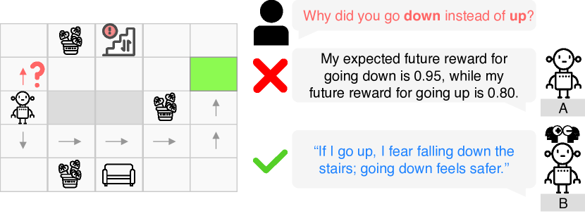
Figure 1: In an interaction between the user and the agent, the user expected the agent to go up, but the agent went down instead. The user asks the system for an explanation. The figure shows two types of explanations the user can receive. (A) is an explanation that can be derived directly from the agent’s policy. (B) is an explanation that can be derived from the agent’s policy with the assistance of additional models called negative and positive influence predictors.

Reinforcement Learning (RL) techniques are becoming increasingly popular in critical domains such as robotics and autonomous vehicles. However, applications such as autonomous cars and socially assistive robots in healthcare and home settings are expected to interact with non-AI experts. People often seek explanations for abnormal events or observations to improve their understanding of the agent and better predict and control its actions [1]. This need for an explanation will likely arise when interacting with these systems, whether it is a car taking an unexpected turn or a robot performing a task unconventionally. Without an explanation, users can find it difficult to trust the agent’s ability to act safely and reasonably  [2], especially if they have limited artificial intelligence expertise. This can even be in the case where the agent is operating optimally and without failure; the agent’s optimal behavior may not match the user’s expectations, resulting in confusion and lack of trust. Therefore, RL systems need to provide good explanations without compromising their performance. To address this need, explainable RL has become a rapidly growing area of research with many open challenges [3, 4, 5, 6, 7, 8, 9].

But what makes a good explanation for end-users who cannot change the underlying model? How do we generate explanations if we cannot modify the underlying RL model or degrade its performance? In RL, an agent learns dynamically to maximize its reward through a series of experiences interacting with the environment [10]. Through these interactions, the agent builds up a model of utility, $Q(s,a)$, which estimates the future reward that can be expected to be achieved if a particular action $a$ is performed from a particular state $s$.

While an RL agent learns from its experiences during training, those experiences are inaccessible after their training is over [4]. This is because $Q(s,a)$ summarizes future experiences as a single, real-valued number; this is all that is needed to execute a policy $\pi=\mathrm{argmax}_{a}Q(s,a)$. For example, consider a robot that receives a negative reward for being close to the stairs and thus learns that states along an alternative route have higher utility. When it comes time to figure out why the agent executed one action trajectory over another, the policy is devoid of any information from which to construct an explanation beyond the fact that some actions have lower expected utility than others.

Explanations need not only address agents’ failures. The user’s need for explanations can also arise when the agent makes an unexpected decision. Requests for explanations thus often manifest themselves as “why-not” questions referencing a counterfactual: “why did not the agent make a different decision?” Explanations in sequential decision-making environments can help users update their mental models of the agent or identify how to change the environment so that the agent performs as expected.

We propose a technique, Experiential Explanations, in which deep RL agents generate explanations in response to on-demand, local, counterfactuals proposed by users. These explanations qualitatively contrast the agent’s intended action trajectory with a trajectory proposed by the user, and specifically link agent behavior to environmental contexts. The agent maintains a set of models—called influence predictors—of how different sparse reward states influence the agent’s state-action utilities and, thus, its policy. Influence predictors are trained alongside an RL policy with a specific focus on retaining details about the training experience. The influence models are “outside the black box”, but provide information with which to interpret the agent’s black-box policy in a human-understandable fashion.

Consider the illustrative example in Figure 1 where the user observes the agent go down around the wall. The user expects the agent to go up, but the agent goes down instead. The user asks why the agent did not choose up, which appears to lead to a shorter route to the goal. One possible and correct explanation would be that the agent’s estimated expected utility for the down action is higher than that for the up action. However, this is not information that a user can easily act upon. The alternative, experiential explanation, states that up will pass through a region that is in proximity to dangerous locations. The user can update their understanding that the agent prefers to avoid stairs. The user can also understand how to take an explicit action to change the environment, such as blocking stairs. Our technique focuses on post-hoc, real-time explanations of agents operating in situ, instead of pre-explanation of agent plans [11], although the two are closely related.

We evaluate our Experiential Explanations technique with studies with human participants. We show that explanations generated by our technique allow users to better understand and predict agent actions and are found to be more useful. We additionally perform a qualitative analysis of participant responses to see how users use the explanations in our technique and baseline alternatives to reason about the agent’s behavior, which not only provides evidence for Experimental Explanations, but provides a blueprint to understand the human factors of other explanation techniques.

2 Background and Related work

Reinforcement learning is an approach to learning in which an agent attempts to maximize its reward through feedback from a trial-and-error process. RL is suitable for Markov Decision Processes, which can be represented as a tuple $M=\langle S,A,T,R,\gamma\rangle$ where $S$ is the set of possible world states, $A$ is the set of possible actions, $T$ is the state transition function, which determines the probability of the following state $P(S)$ as a function of the current state and action. $T:S\times A\rightarrow P(S)$, $R$ is the reward function $R:S\times A\rightarrow R$, and $\gamma$ is a discount factor $0\leq\gamma\leq 1$. RL first learns a policy $\pi:S\rightarrow A$, which defines which actions should be taken in each state. Deep RL uses deep neural networks to estimate the expected future utility such that $\pi(s)=\operatorname*{argmax}_{a}Q_{\theta}(s,a)$ where $\theta$ are the model parameters.

As deep reinforcement learning is increasingly used in sensitive areas such as healthcare and robotics, Explainable RL (XRL) is becoming a crucial research field. For an overview of XRL, please refer to Milani et al. [8]. We highlight the most relevant work on XRL to our approach.

Rationale generation [12] is an approach to explanation generation for sequential environments in which explanations approximate how humans would explain what they would do in the same situation as the agent. Rationale generation does not “open the black box” but looks at the agent’s state and action and applies a model trained from human explanations. Rationales do not guarantee faithfulness. However, our models train alongside the agent and achieve a high degree of faithfulness.

Some XRL techniques generate explanations by decomposing utilities and showing information about the components of the utility score for an agent’s state [13, 14, 15, 16]. Our technique is related to decompositions in that we learn the influence of different sources of reward on utilities, avoiding the trade-off between using a semi-interpretable system or a better black-box system.

Our work focuses on counterfactual explanations, but we differ in the explanation goals and approach from other works. For example, Frost et al. [17] trained an exploration policy to generate test time trajectories to explain how the agent behaves in unseen states after training. Explanation trajectories help users understand how the agent would perform under new conditions. While this method gives users a global understanding of the agent, our method focuses on providing local counterfactual explanations of an agent’s action. Contrastive approaches such as van der Waa et al. [18] leverage an interpretable model and a learned transition model. Madumal et al. [19] explain local actions with a causal structural model as an action influence graph to encode the causal relations between variables. Sreedharan et al. [20] generate contrastive explanations using a partial symbolic model approximation, including knowledge about concepts, preconditions, and action costs. These methods provided answers to user’s local why not questions. Our approach minimizes the use of predefined tasks or a priori environment knowledge.

Olson et al. [21] explains the local decisions of an agent by demonstrating a counterfactual state in which the agent takes a different action to illustrate the minimal alteration necessary for a different result. Huber et al.[22] furthers this concept by creating counterfactual states with an adversarial learning model. Our technique, however, concentrates on the qualitative distinctions between trajectories and not on the states.

3 Experiential Explanations

Experiential Explanations are contrastive explanations generated for local decisions with minimal reliance on structured inputs and without imposing limitations on the agent or the RL algorithm. Our explanation technique uses additional models called influence predictors that learn how sparse rewards affect the agent’s utility predictions. In essence, influence predictors tell us how strongly or weakly any source of reward (positive or negative) is impacting states in the state space that the agent believes it will pass through. This is in contrast to the agent’s learned policy, which aggregates the utilities with respect to all rewards. This enables agents that use our explanation technique to provide additional context to the choices they make because it knows about their utility landscape in finer-grained detail. As in Figure 1, we see the explanation referencing the agent’s relationship to the environment in terms of negative and positive elements.

Once we have trained these influence predictor models, explanation generation proceeds in two phases. First, given a decision made by the agent and a request for an explanation, we generate a state-action trajectory that the agent will take to maximize the expected reward plus a counterfactual trajectory based on the user’s expectation. For example, in Figure 1 the agent’s trajectory is down, but the user asks about going up.

Second, we use influence predictors to compare the two trajectories and extract information about the different influences along each. In the following sections, we will dive into the details about the influence predictors, what they are, how we train them, how to use them to generate explanations, and the other components of the explanation generation system and how we generate explanations.

3.1 Influence Predictors

Influence predictors reconstruct the effects of the received rewards on utility during training. These models are trained alongside the agent to predict the strength of the influence of different sources of reward on the agent: $U_{c}(s,a)$ where each $c\in C$ is a distinct source (or class) of reward. For example, a terminal goal state might be a source of positive reward, stairs might be a source of negative reward, and other dangerous objects may be other sources of negative reward. In a more complex environment, multiple sources of positive and negative rewards can be helpful to outline the agent’s plan. For instance, a robot attempting to make a cup of coffee would receive positive rewards for obtaining a clean mug, hot milk and coffee, then combining the milk and coffee in the mug and stirring them. Negative influences could include getting a dirty cup or adding salt.

In principle, any agent architecture and optimization algorithm can be used with our explanation technique as long as we can observe its transitions during training. Influence predictors are trained similarly to an RL agent (e.g., standard Deep $Q$-networks (DQN) [23], or A2C [24]) but with two differences. First, during training, each influence predictor model can only receive rewards from one class of rewards. Influence predictors are trained using loss based on a modified Bellman equation: $U_{c}(s_{t},a_{t})=|r^{c}_{t+1}|+\gamma\max_{a^{\prime}}U_{c}(s_{t+1},a^{\prime})$ where $r^{c}_{t+1}$ is the reward associated with $c$ delivered to the agent upon transition to state $s_{t+1}$. The absolute value re-interprets the reward as an influence, since the influence predictor is now predicting the utility of attaining the reward, even if it is negative. As a consequence of ever receiving only the absolute value of a class of rewards, $U_{c}(\cdot)$ is an estimate of the strength of $c$ in $s$ and $a$.

Second, influence predictors are not used to guide the agent’s exploration during training or inference. They rely on the main policy’s training loop to generate transitions.

Each source of reward has its own influence predictor model. Typically, one class is associated with a goal state (or states required for task completion) and produces positive rewards. Sometimes an intermediate positive reward is given when it is known in advance that the task requires particular actions or states to be traversed, as in the case of reward shaping [25]. Other classes are associated with states that are detrimental to the task and produce negative rewards.

The training process for influence predictors is shown in Algorithm  1. The agent, controlled by its base policy learning algorithm, interacts with the environment, executing actions and receiving state observations. State transitions, actions, and rewards are recorded and used to populate separate replay buffers for each influence predictor. Each time step, we sample each replay buffer and backpropagate loss in each influence model.

Algorithm 1 Influence predictor and agent training

for each $c\in C$  do $\triangleright$ $C$ is the reward sources

    Initialize buffer memory $D_{c}$ to capacity $N$

    Initialize action-value function $U_{c}$ with random weights

end for

for episode = 1, M do

    $transitions_{T}\leftarrow agent.transitions(T)$ $\triangleright$ The agent’s transition data from its buffer

    for t=0, T do

       for each $c\in C$ do

          if $reward_{t}\in c$ then

             $transitions_{T}[t][reward]\leftarrow\lvert transitions_{T}[t][reward]\rvert$

          else

             $transitions_{T}[t][reward]\leftarrow 0$

          end if

          $(transitions_{T}[t])\to D_{c}$

       end for

    end for

    for each $c\in C$ do

       $U_{c}\leftarrow update(D_{c})$

    end for

    $agent\leftarrow update(transitions_{T})$

end for

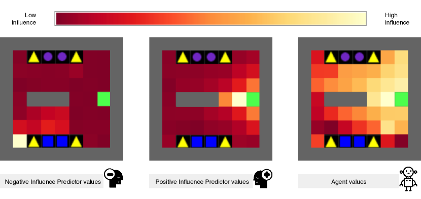
Figure 2: This figure shows an example of the agent’s learned maximum learned utility value at each state and the two influence predictors values visualized on heatmaps. The blue squares are the source of negative rewards, whereas the green square is the source of positive rewards. The purple and yellow shapes have no effect. Intuitively, one can see that the agent’s policy (right) is closely associated with the positive influence values and the opposite of the negative influence values.

To illustrate, Figure 2 shows an agent operating in an environment with two reward classes: a positive reward class for the terminal goal, and a negative reward class for the blue squares. The influence map on the left was generated by querying the negative influence predictor for each state and maxing across all possible actions. The negative influence trends are stronger closer to the blue squares. The influence map in the middle is generated from the positive influence predictor. The map on the right is the agent’s main policy model, trained on all reward classes as normal. Even though the visualization aggregates action utilities, one can see that the agent will prefer a trajectory in the upper part of the map.

3.2 Explanation Generation

At any time during the execution of the policy, the user can request a counterfactual explanation by proposing an action $(a_{\mathrm{U}})$ rather than the one the agent chose $(a_{\mathrm{A}})$. Given the action chosen by the agent and the alternative action proposed by the user, the explanation generation process proceeds in three phases.

First, we generate and record the trajectory $\tau_{\mathrm{A}}$ the agent will take from this point forward. Second, we generate a counterfactual trajectory $\tau_{\mathrm{U}}$ as if the agent had executed the user’s proposed alternative action. To generate $\tau_{\mathrm{U}}$, we force the agent to follow the user’s suggested alternative action (or sequence of actions in the case that the user wants to specify a partial or complete counterfactual trajectory) and complete the trajectory using the same planning approach.

Finally, we use influence predictors to compare the two trajectories. Recall, in Section 3.1, we have an influence predictor $IP_{c}$ per reward source $c\in C$. We have access to all the influence predictor values in both trajectories at this stage, which gives us control over the types of explanation we can generate depending on our use case. We can produce local, detailed, global, or aggregated explanations. Furthermore, explanations can be enriched by giving names to reward states and textual descriptions of the consequences of visiting a reward state (e.g., “stairs” and “fall down”, respectively). In this work, we explore two variants of the explanations: an aggregated explanation and a detailed local explanation.

Aggregated Explanation. An aggregated explanation presents an overview of the effect of each reward class on the agent throughout a complete trajectory. To generate these explanations, we calculate the mean value of each influence predictor $IP_{c}$ for all states $s\in\tau_{\mathrm{A}}$ and compare this mean with the other trajectories

$$\operatorname*{argmax}_{a\in\{a_{\mathrm{U}},a_{\mathrm{A}}\}}(\frac{\sum_{s}{\max(IP_{c}(\tau_{\mathrm{a}}[s]))}}{length(\tau_{\mathrm{a}})}),\forall c\in C.$$

The resulting explanation assigns each influence predictor to the trajectory in which they were the most dominant. We then take these values and translate them into English explanations. If the values generated by $IP_{c}$ were similar for both trajectories, then they can be excluded from the explanation, as they do not provide valuable information. For example, in the case of two influence predictors in a simple environment, if we assume that we only got a difference in the negative influence predictor. The explanation would be as follows: “If I go up, I fear falling down the stairs; going down feels safer”. This case is demonstrated in Figure 1. Suppose that there is a difference in an additional $IP_{c}$ mean. In that case, we add it to the explanation by appending its relevant sentence to explain all influence predictors if we observe a difference in their mean values.

Local Explanation. In more complex environments where there are many influences, the explanations can shed light on the agent’s near-horizon and concentrate more on exploring local values. These local explanations zoom in on the most influential factors related to actual and counterfactual actions over their corresponding segments, which are denoted by $t_{\mathrm{A}}\subseteq\tau_{\mathrm{A}}$. Each segment starts at the beginning of the designated action and includes a pre-determinted number of additional steps (we used five steps) after the end of the action to capture some of the longer-term effects.

To generate a local explanation, we first identify the most significant factors for each local segment by calculating the maximum influences of each state $s$ during a segment:

$$\{\operatorname*{argmax}_{c\in\{C\}}(\max{(IP_{c}(s))})|\forall a\in\{a_{\mathrm{U}},a_{\mathrm{A}}\},\forall s\in t_{\mathrm{a}}\}$$

From the result, we obtain a set that includes all unique influence predictors $IP_{c}$ that had a maximum value at any point of the segment. If there is no difference between the segments of $a_{\mathrm{A}}$ and $a_{\mathrm{U}}$ with respect to their sets of maximum influences $IP_{c}$, we resolve to compare the mean values of the influence predictors during the same period and obtain the three influences with the highest means in their segments. First, we get the mean of every influence predictor in each segment:

$$mean(IP_{c},a)=\frac{\sum_{s}{\max{(IP_{c}(t_{\mathrm{A}}[s]))}}}{||t_{\mathrm{A}}||},\forall c\in C,\forall a\in\{a_{U},a_{\mathrm{A}}\}$$

Then, we obtain the top three influences for each segment $t_{\mathrm{A}}$ and $t_{\mathrm{U}}$, ordered by $mean(IP_{c})$.

We provide this explanation even if there is no difference in the top influences, which can happen if the alternative action considered is too similar to the actual action taken. To generate English explanations, we utilize the list of top influence predictors obtained through either the maximum or highest mean method. An example of a generated explanation can be: “If I got the nearby cup, I would still have to clean it before making my coffee. But if I get a cup from the cupboard, I will not need to clean it and I can immediately make coffee.”

The explanation strategies mentioned above provide information about how external environmental rewards affect the choices made by the agent, even if they are not directly linked to the agent’s actions. These explanations are in line with the definition of first-order explanations [27], as they reveal the underlying inclinations of the agent towards the environment and other factors that influence its decisions.

4 Evaluation overview

Our evaluations focus on exploring how beneficial experiential evaluations are to people, and how people use explanations to reason about their own decisions through quantitative and qualitative analyses. Our human evaluations address the following research questions:

• Do Experiential Explanations improve the users’ predictions of the agent’s actions over baselines?

• Do users find experiential explanations satisfactory compared to baselines?

• What features of the explanations do users perceive as helpful in predicting agent actions?

• Are the explanations effective in more complex domains?

We also examined the faithfulness (RQ 5) of our explanation system automatically by looking at how closely the influence predictor’s values estimate the agent’s actions.

In the following sections, we detail the two environments on which we evaluated our explanations. The first is the MiniGrid environment, where we examine the performance of a global version of the explanations in a sparse-reward setting with two reward classes. In the second study, we use the Crafter environment to explore the effectiveness of the local explanations generated by our method in a more complex environment with sequential multi-step goals, along with more granular reward classes. Moreover, we want to see if the local Experiential Explanations can convey these complex values to the participants coherently.

5 Experiment 1: MiniGrid Environment

In this study, we evaluate our explanations in an environment with two simple reward sources and simplified grid-navigation settings, with only one possible counterfactual action at the decision point (see Figure 3). Our aim is to answer our research questions (RQ1, RQ2, and RQ3) where we evaluate the performance of our explanation method with quantitative and qualitative analyses. We additionally automatically validate the faithfulness of the explanations through automated tests (RQ5). We built our experimental domain on MiniGrid [28], a popular minimalistic grid world environment that offers a variety of tasks to test RL algorithms.

5.1 Model Setup and Environment Details

Environment customization. We require an environment with multiple reward classes—positive rewards as well as one or more sources of negative rewards—thus we created a custom task where the agent is placed in a room with a goal (a green square) and other objects represented by colored shapes that we could assign to neutral or negative reward values when approached. The environment provides sparse rewards; a positive reward of $(1-\frac{steps}{\text{max allowed steps}})$ for reaching a green goal tile (the minigrid default) and $-1$ for stepping into a dangerous object. Both the goal and stepping on the dangerous object terminate the episode. All other states and actions produce zero reward.

Agent training. Our base agent policy model is the advantage actor-critic (A2C) [29] optimized using the exponential policy optimization algorithm (PPO) [30]. A state observation is an image of the grid constrained by a limited field of view. We include more technical details about the agent’s architecture and training in appendix A.

Influence Predictors design and training. We are using DQNs as our influence predictors (as described in [23]). Specifically, we have two predictors, one for negative rewards and one for positive/goal rewards. We provide more details on the training and architecture of the Influence Predictors in appendix B.

Explanation generation. We use the aggregated explanations described in Section 3.2. These explanations contrast the aggregated difference in the means between the agent’s paths, the one associated with the proposed counterfactual, and the one the agent did. Below are some examples of these explanations:

1. Negative rewards heavily influence the counterfactual trajectory. “If the agent goes down, it will pass through regions influenced by the dangerous blue obstacles; going up feels safer”.

2. Goal rewards have a lower influence on the counterfactual trajectory. “If the agent goes right, it will pass through regions less influenced by the green goal; going left is better”.

5.2 Baselines

In this experiment, we focus on similar global baseline explanations that the agent can generate. We compared our method with the following baselines:

• Heatmap explanation: Showing the agent’s learned maximum values for each state. We generate the explanations for this baseline by getting the maximum agent value in each possible state on the map. This is similar to the agent values map in figure 2.

• Q-Value explanation: Presenting the average expected reward for both paths. These explanations utilize the simulator from our explanation generation pipeline, but not the influence predictors. This baseline is a comparison of the mean agent’s values between the paths. An example of such an explanation is The Q average if the agent goes up 9.84, while the Q average if the agent goes down is 9.66.

• No explanation: The users only saw the correct answer without further explanation.

5.3 Method

We designed our human-participant evaluation following the framework proposed by Hoffman et al. [31], evaluating our system for understandability, performance, and user satisfaction. We conducted our online evaluation between subjects using Prolific with 81 participants aged 21-71 years old (M=37.41, SD=11.03); 39.5% of the participants identified as women. The average study completion time was approximately 10 minutes, and we compensated each participant with $3.75. The study consists of two parts: answering a series of prediction tasks (RQ1, RQ3) and a satisfaction survey (RQ2, RQ3).

In the first part, we presented three episodes to each participant, as shown in Figure 3. During each episode, the agent—the red triangle—must navigate to the green square. Some colored shapes are associated with negative rewards, but the participant is not told which ones. After each episode, the participant is asked to predict whether the agent will go up or down. The participant has no information at the beginning of the first episode to make an informed choice, and the participant choice is random—we do not evaluate on this choice. Further, upon the participant’s choice, we assign which object is dangerous such that the participant is always wrong. This established the conditions for which the participant must now learn to correct their understanding of the agent’s interactions with the environment. We use that assignment of dangerous object consistently throughout the second and third episodes. The participant tries to predict the agent’s choice after the second and third episodes (without the object assignment switching); we expect to see the participants in the experimental condition to have higher accuracy rates than in the baseline conditions.

After each episode, participants fill out a brief text entry question explaining the rationale behind their choice.

The second part of the study was a satisfaction survey consisting of five-point Likert scale questions asking the user to rate understandability, satisfaction, amount of details, completeness, usefulness, precision, and trust for the explanations they saw. It also had an open-ended response question asking how the explanation helped or did not help them understand the agent. Appendix D includes more details about the explanations and survey questions.

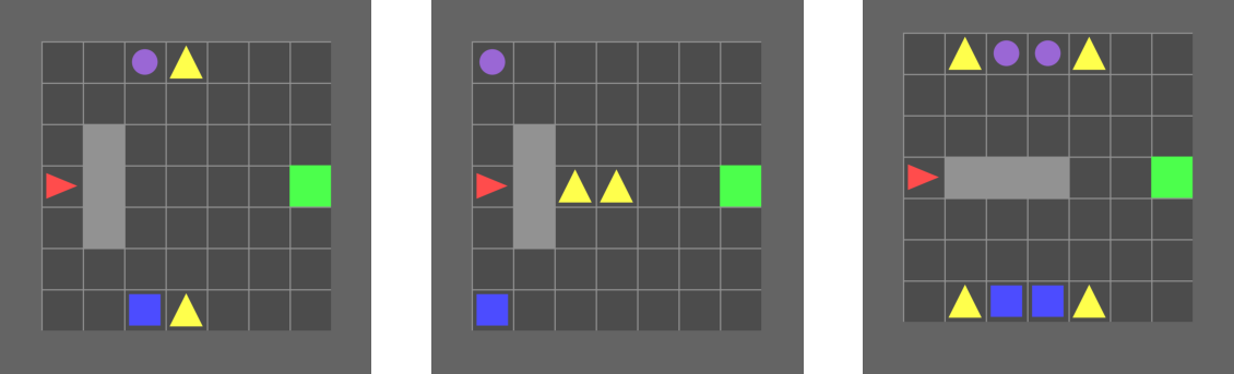
Figure 3: The three episodes from the human study, in order presented to participants.

	$2^{nd}$ Correct	$3^{rd}$ Correct	Both Correct
Experiential Exp.	90.48%	95.24%	85.71%
Heatmap Exp.	78.95%	78.95%	63.16%
Q-value Exp.	80.95%	80.95%	66.67%
No Explanation	75.00%	70.00%	55.00%

Table 1: The percentages of correct answers for first prediction task and second prediction task and the combined percentages.

5.4 Quantitative Results

RQ1: Prediction Correctness. We measure whether the participant can correctly predict the agent trajectory after interacting with the second and third episodes (Figure 3).

Table 1 shows the percentage of correct answers for each type of explanation after the second and third episodes (the first was a control), as well as the combined average. Participants provided with Experiential Explanations had the highest success rate. Experiential Explanations were significantly higher than the no-explanation condition, validated with a logistic regression $(p<0.05,df=3,\chi^{2}=4.404)$. Experiential Explanations led to a 9.5+% improvement over other baselines, but were not statistically significant at the same threshold.

RQ2: Satisfaction Survey. For each type of explanation, we analyzed the ratings of the participants for the Likert scale questions on the satisfaction survey. Experiential Explanations had the highest average scores on all dimensions, except trust. A one-way analysis of variance (ANOVA) followed by Tukey’s honestly significant difference test revealed that the Experiential Explanations $(M=3.62,SD=1.32)$ were preferred over the Heatmaps $(M=2.42,SD=1.35)$ in completeness ($F(3,81)=3.032,p<0.05$). Experiential Explanations $(M=3.71,SD=1.0)$ were preferred over the Heatmaps $(M=2.63,SD=1.38)$ in satisfaction($F(3,81)=3.106,p<0.05$). Experiential Explanations $(M=4.38,SD=0.59)$ were preferred over Q-Value Explanations $(M=3.28,SD=1.01)$ and Heatmap Explanations$(M=3.0,SD=1.37)$ in the dimension of understandability ($F(3,81)=5.572,p<0.05$).

5.5 Qualitative Analysis

To address RQ3, we thematically analyzed open response questions for the tasks and satisfaction survey to better understand how the participants used the explanations. Thematic analysis is one of the most common qualitative research methods and involves identifying, analyzing, and reporting patterned responses or meanings (i.e. themes) [32]. It is most appropriate for understanding a set of experiences, thoughts, or behaviors across data [33]. To conduct the thematic analysis for each of these codes, three authors performed the following established process, as outlined by [32]: (1) We familiarized ourselves with the data through repeated active readings. (2) We developed a coding framework consisting of a set of codes organizing the data at a granular level and the corresponding well-defined and distinct definitions. (3) Each of the authors independently coded the entirety of the data. If a code was unclear or a new code was needed, the authors consulted with each other to modify the coding framework. If a change was made, each author independently re-analyzed the entirety of the data. (4) We jointly examined the codes to derive themes and findings. We compared our application of the codes for each response to ensure consistency. Discrepancies were counted and used to calculate the inter-rater reliability. The process iterated until all discrepancies were resolved. We identified three themes: Usefulness, Format, and Utilization.

Explanation Usefulness. The theme of Usefulness emerged in the open-ended comments about how participants perceived the explanations. Because these comments were made alongside users’ explanations of their reasoning, this provides additional information on how useful users found the explanations. We identified three Usefulness codes: Useful, Not Useful, and Unclear. We coded a response Useful if a participant explicitly mentioned that the explanation was useful, for example, “I understood that purple was dangerous and that the agent should avoid getting near it (EE8).” Responses were coded Not Useful if a participant explicitly stated that the explanation was not useful, for example, “I tried to read the chart but found it confusing and unclear. I didn’t understand it very well (HE10).”. Responses were coded Unclear if the user’s perception was ambiguous, for instance, “I found the explanations a bit too brief. For instance, what makes the purple circles feel safer than the blue squares (EE7)?” The initial inter-rater reliability for Usefulness was 81.5%.

Table 2 shows participants’ perceived Usefulness across explanation types according to usefulness codes. Experiential Explanations were considered Useful most often. Heatmap explanations were considered Not Useful most often, even more than when No Explanation was provided. A logistic regression comparing the Usefulness of each explanation showed Experiential Explanations were 9 times more likely to be found useful than Heatmap explanations and 4 times more likely than Q-value explanations ($p<0.05$, $df=3$, $\chi^{2}=14.99$). We also note that 88.89% of the participants who thought the explanations were useful predicted correctly in both questions, indicating the correlation between correctness and usefulness ($p<0.05$, $df=2$, $\chi^{2}=9.33$).

Explanation Format. Participant responses were also coded for Format. We derived three codes for Format: Need More Information, Hard to Understand, and Suggestion. Responses coded as Need More Information explicitly stated why the explanation was lacking and what data was desired. If the response said that the explanation was not clear, it was coded as Hard to Understand, and if the response offered another way to explain, it was coded as Suggestion. Only responses from individuals who received explanations and referenced the explanation’s content could be coded for Format (41.98% of our dataset). Participants often expressed a Need for More Information when shown Heatmap explanations, followed by Q-value explanations. Participants who did not find the explanations useful had more Format comments. The initial inter-rater reliability was 76.47%.

	Useful	Unclear	Not Useful
Experiential Exp.	80.95%	19.05%	0.00%
Heatmap	31.58%	31.58%	36.84%
Q-value Exp.	47.62%	14.29%	38.10%
No Explanation	N/A	N/A	N/A

Table 2: Participant’s rates of usefulness for each explanation type.

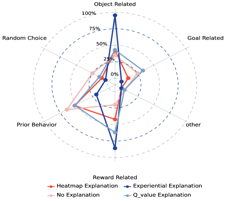
Figure 4: The distribution of themes over the different explanation types. Participants who saw Experiential Explanations, which presented Object Related and Reward Related information, relied more heavily on the kinds of information it provided than other explanation types. Q-Value and Heatmap explanations both presented Reward Related information. The breakdown of themes for the heatmap and q-value explanations more closely resemble the no-explanation case.

Explanation Utilization. Utilization refers to whether the participant made use of the information available within the explanation to reason about what the agent will do. We extracted the following codes for the types of information participants referenced in their rationales: Object Related (e.g., shapes or colors); Reward Related (e.g., “safer”, “higher”, or “lower” rewards); Goal Related (e.g., distance / direction to goal); Prior Behavior (e.g., references behavior from prior outcomes); Random Choice (e.g., no clear justification); and Other (e.g., references other factors such as obstructions). The inter-rater reliability of the initial coding was 75.6%.

We compared the frequency with which utilization codes appeared in open-responses. If a participant used the same types of information as the explanation provided, we considered the participant as “Utilizing” the explanation. Experiential Explanations provide Object and Reward Related information. Heatmap and Q-Value Explanations provide Reward-Related Explanations. No Explanation only provides for Prior Behavior. 71% of the participants who were shown Experiential Explanations utilized the exact kinds of information presented in the explanation, compared to 21% and 28% for the Heatmap and Q-Value explanations, respectively. Although the Q-Value and Heatmap explanations both presented Reward-Related information, participants still relied heavily on Prior Behavior to understand the agent. Experiential Explanations were 13 and 15 times more likely to have the information they provided be Utilized and Useful with respect to Heatmap and Q-Value explanations, respectively. We also found that among those who used components of explanations in their reasoning, 55.88% answered correctly on both questions ($p<0.05,df=1,\chi^{2}=3.849$). But within the Experiential Explanations group, the percentage was 84.62% and that group was more statistically significant to get both questions correctly than other baseline explanation groups ($p<0.05,df=3,\chi^{2}=12.22$).

Figure 4 shows the distribution of the reasons the participants referenced for each type of explanation. Participants who saw Experiential Explanations most used Object-related and Reward-Related information. Participants who saw Q-Value explanations referenced Goal-Related reasons the most. Participants who saw no explanation most often utilized Prior Behavior, followed by Object-Related reasons. Notably, participants who saw Experiential Explanations were 4 times less likely to rely on Prior Behavior, indicating they did not rely as much on watching the agent to understand it. Those who saw Heatmap and Q-Value Explanations relied heavily on Prior Behavior and Utilization patterns mimicking those of the No Explanation condition.

5.6 Faithfulness Evaluation

To address RQ5, a key consideration of explanation generation is the extent to which the explanations are faithful to the underlying system [34]. Influence predictors sit “outside of the black-box”, which is the policy model that drives the agent. However, influence predictors are trained alongside the main policy model, and thus, if they learned correctly, should be able to estimate the agent’s actions with a high degree of accuracy. We don’t expect them to replicate the agent’s actions as they are learning influences instead of generating actions. To assess the faithfulness of influence predictors, we evaluated the accuracy of influence predictors’ combined decision in predicting the agents.

To calculate the faithfulness, we combine the predictions of the influence models using two methods. The first is by taking the $action=\operatorname*{argmax}_{a}(\sum_{i}P_{i}(s,a)-\sum_{j}N_{j}(s,a))$ where $P_{i}$ is a positive influence predictor and $N_{j}$ is a negative influence predictor. The second method is to train a classifier on the predicted positive and negative influence values as features and the agent’s actions as the ground truth. We used an SVM classifier with an RBF kernel. We also examined how the predictors’ accuracy changed in critical regions; when influences were stronger than specified influence thresholds.

For our first test, the accuracy of the influence models in predicting the agent’s actions, we found the accuracy of the prediction of the direct aggregation is $72\%$ and the accuracy of the classifier $76\%$. In certain critical states where at least one influence predictor exceeded a threshold of $0.100$, the aggregate of influence predictors agreed with the main policy $83\%$, covering at least $20\%$ of the environment. At higher thresholds, agreement jumps above $90\%$ indicating that when decisions are the most important, faithfulness is very high. Looking at the positive influence predictor alone, at a threshold of $0.200$ and higher, it alone can predict the agent with a $100\%$ accuracy. This is to be expected as the influence predictors cannot dictate what states and actions get explored—it is controlled by the main policy and the main training algorithm—so states that are less critical to positive reward attainment are under-sampled and prone to more error in both the main policy and the influence predictors.

6 Experiment 2: Crafter Environment

This experiment is designed to evaluate the Influence Predictors in a visually richer environment, with more decision points and options, along with multiple reward classes. And, as before, we will validate the faithfulness through automated testing.

To create such a setting, we used the Crafter environment developed by Hafner [35], a 2D version of the game, MineCraft with the same rules for interacting with the environment and crafting new tools. Crafter can generate 2D open-world survival environments with randomized maps. These environments consist of varying terrains, a day-night cycle, as well as interactable materials, objects, and living entities. Crafter also supports an on-screen inventory, allowing an agent to collect items in order to construct a variety of items later. An agent playing Crafter needs to complete various tasks in a sequential order, while maintaining its health by obtaining resources and avoiding threats.

6.1 Model Setup and Environment Details

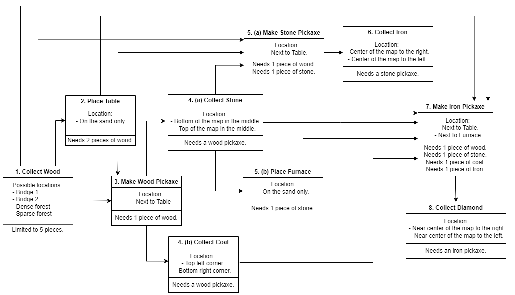
Figure 5: Depiction of the Digger’s quest, listing the achievements that the Digger needs to attain and the order in which that needs to be done

Environment Customization. We needed a good distribution of positive and negative reward sources. Crafter provides multiple sources of positive rewards, but the only negative rewards come from health depletions. To counter this and to add a conceptual narrative, we created an agent persona, called the Digger, whose aim is to obtain a diamond. The Digger’s reward system provides positive rewards for achievements related to digging, such as acquiring resources to construct digging tools, creating these tools, and digging for minerals. We provide negative rewards if the agent strays from the Digger persona, for example, by constructing weapons, or killing an entity. Figure 5 depicts the sequence of achievements required to reach a diamond.

Additional customizations were added to optimize the training process. The world map was made static, so that the agent could find all required resources in a limited number of steps while making it easier for a participant to understand the world map. No rewards were given for performing actions to maintain health, such as drinking water, but improvement or depletion of health had correponding positive and negative rewards. While all other achievement rewards are in the range of +1 to -1, diamond collection has a +50 reward to focus the agent’s training exploration towards getting a diamond. Finally, a small bonus is given for reaching the diamond in fewer timesteps, to improve agent performance.

Agent training. The agent needs to learn to traverse the map, completing the achievements required to reach the diamond in a small number of timesteps. At any given point, its observation consists of an image of its surroundings inside a limited field of view along with its current inventory. Given a static map, the agent is trained from various starting points to aid in the training exploration. We use on-policy learning algorithms for the agent, implementation details for which are available in appendix C.

Influence Predictor design and training. For the Crafter experiment, we attached Influence Predictors (IP) to achievement categories. Each predictor was responsible for tracking either favorable achievements leading to positive rewards or unfavorable achievements leading to negative rewards. The Health-tracking IP was the only exception here, as it tracked both improvement and depletion of health, resulting in rewards that are sometimes positive and sometimes negative. Table 3 lists all Influence Predictors, along with the achievements they track.

Influence Predictor	Reward type	Achievements
Coal collection	Positive	collect-coal
Diamond collection	Positive	collect-diamond
Iron collection	Positive	collect-iron
Stone collection	Positive	collect-stone
Wood collection	Positive	collect-wood
Iron pickaxe construction	Positive	make-iron-pickaxe
Stone pickaxe construction	Positive	make-stone-pickaxe
Wood pickaxe construction	Positive	make-wood-pickaxe
Furnace placement	Positive	place-furnace
Table placement	Positive	place-table
Murder tracking	Negative	defeat-zombie
Iron sword construction	Negative	make-iron-sword
Stone sword construction	Negative	make-stone-sword
Wood sword construction	Negative	make-wood-sword
Health tracking	Positive and Negative	life-maintenance, collect-drink, eat-cow

Table 3: Complete list of Influence Predictors with the achievements that they track and their corresponding reward types

The Influence Predictors were also trained using on-policy learning, the technical details can be found in appendix C. The predictors were given full access to the agent’s rollout buffer allowing them to see the agent’s observation space, action taken, and reward obtained, along with whether the episode just started and the probability distribution of agent’s actions. IPs would only read the rewards pertaining to their own achievements and consider rewards from other sources as 0. Also, instead of taking the actual reward, IPs read the magnitude of the reward to track the intensity of influence of their achievements, irrespective of whether they are positive or negative. The Health-tracking IP would also consider the sign of its reward, given that health can be both positive and negative. The predictor models calculated the value and subsequently the advantage and results using their own respective critics. They would then populate their own rollout buffers with these details and train on the same. Each IP hence would learn its individual policy based on the agent’s explorations.

We explored the IP values by standardizing them to compensate for reward variations and obtained graphs such as Figure 6. We see that the influence of rewarded states associated with achievements keep rising until the achievement was obtained and drop immediately after, leading to creation of spikes as visual indicators of when an achievement was made. The IPs hence expose the user to knowledge about the agent’s goal hierarchy because the positive rewards are attached to achievements. This is something that we don’t see in the simpler minigrid and a useful emergent property of the technique.

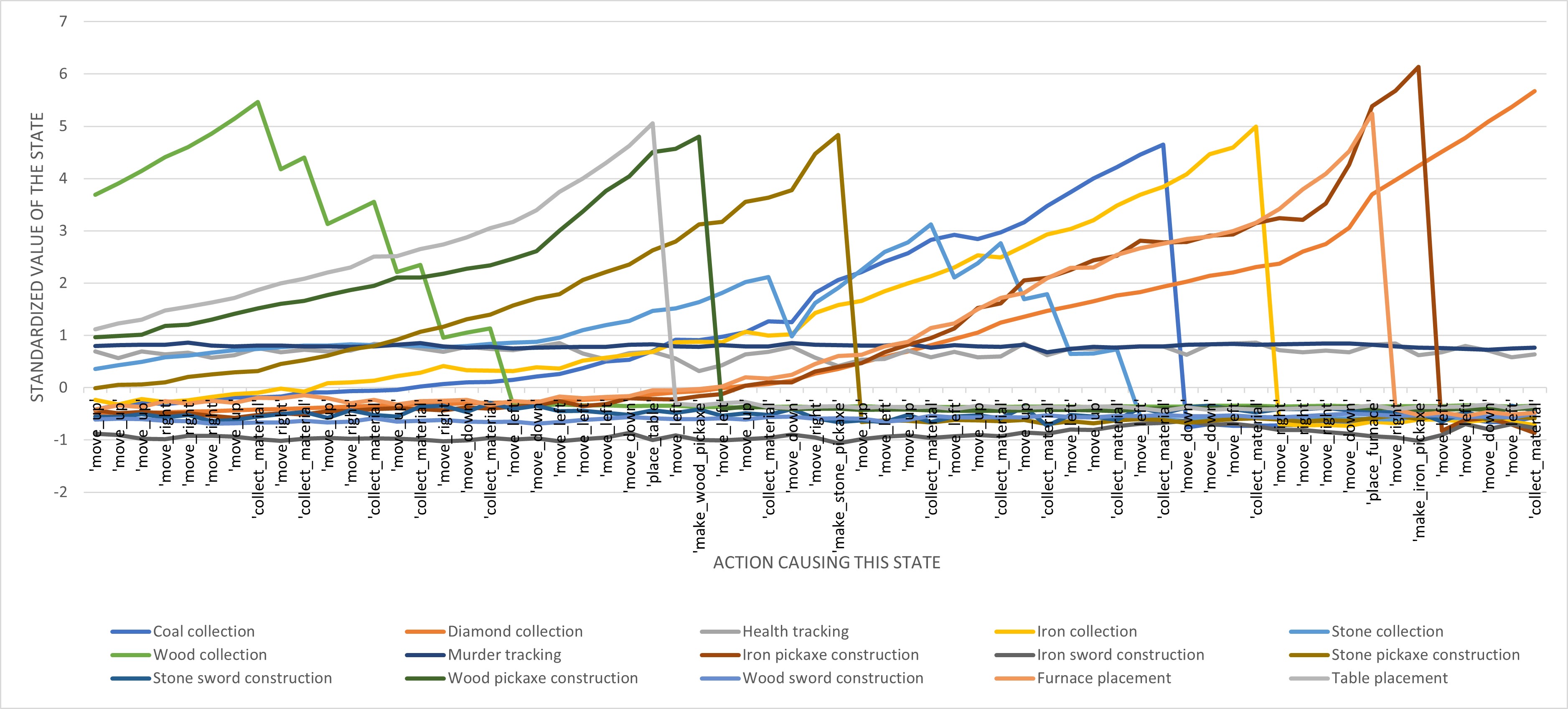
Figure 6: A plot of the standardized values of a given state according to individual Influence Predictors, the x axis shows the action names after which a given state was achieved.

Explanation generation. To explain the actions of the agent, we provide local explanations that narrate what the agent plans to do next after the actual or counterfactual action, as described in Section 3.2. An example of such an explanation would be: “The agent needed wood and chose to get it from the sparse forest. This led to the prioritization of building a table, building a stone pickaxe, and getting stones next. However, if it had gotten to the dense forest, it would have to think about owning a wooden pickaxe, fearing for its health and avoiding dangerous zombies instead.” This explanation conveys that the dense forest is a more dangerous option for the agent, because the agent knows, while the user might not, that there are zombies roaming around that forest and it would be wiser to get wood from the safer sparse forest.

6.2 Faithfulness Evaluation

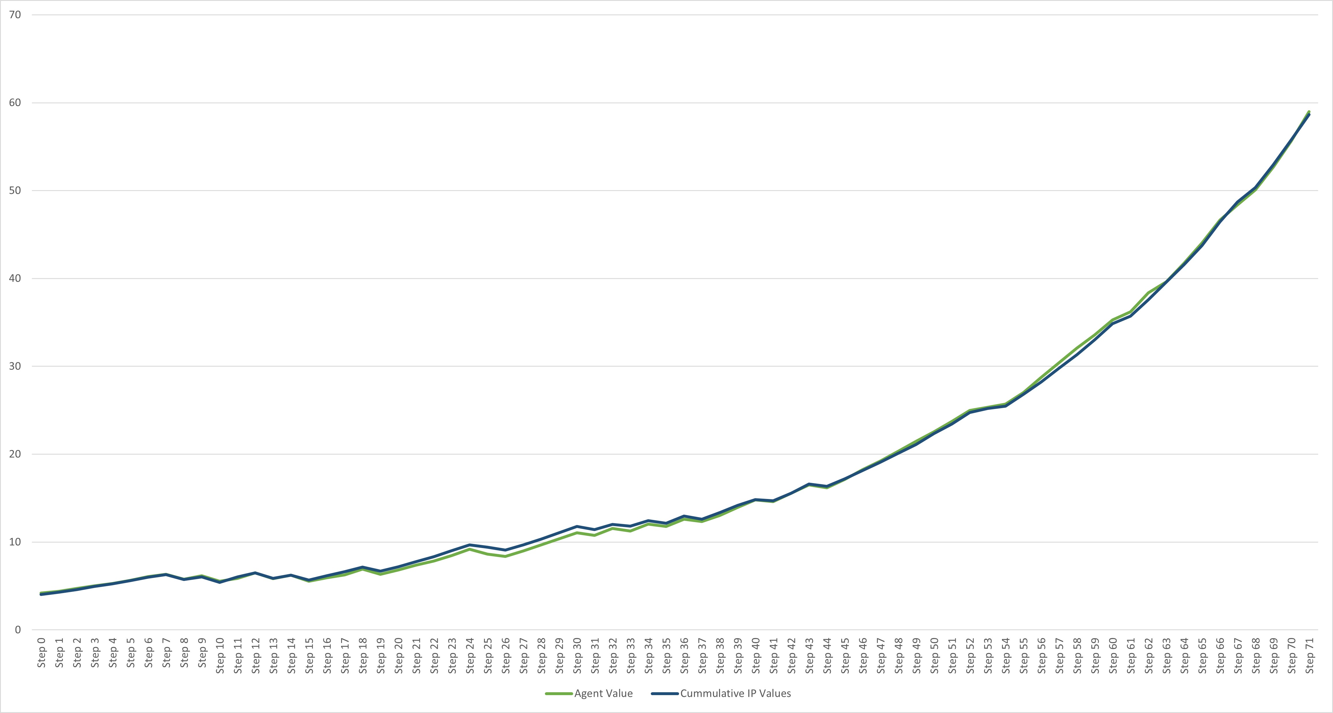
Figure 7: This plot depicts the values of different states as traversed by the agent during a successful test run. The green line represents the values according to the agent’s learned policy. The deep blue line depicts the cumulative values according to the policies learned by the Influence Predictors. Both plots match almost exactly, meaning that the policies learned by the Influence Predictors align closely with the policy learned by the agent.

To determine faithfulness, we plotted the agent’s values corresponding to each state. We also plotted the sum of values of the same states according to the IPs using the formula:

$$\text{Cumulative IP value}=\sum_{p\_ip\in P}{(p\_ip\rightarrow value)}-\sum_{n\_ip\in N}{(n\_ip\rightarrow value)}$$

where $P$ is the set of positive IPs including Health tracking IP and $N$ is the set of negative IPs. The plots aligned almost perfectly, as demonstrated in Figure 7, which depicts a test run of average length.

We also calculated the Root Mean Squared Percentage Error (RMSPE) [37] between the agent values and the cumulative IP values for a set of 9 test runs. These runs used the same trained agent on the same map, but varied the starting location. RMSPE is calculated as:

$$RMSPE=\sqrt{\frac{1}{N}\sum_{n=1}^{N}{\left(\frac{\hat{y}_{n}-y_{n}}{y_{n}}\right)}^{2}}$$

RMSPE values averaged 3.13%, indicating a high similarity between the agent policy and the cumulative IP values.

7 Conclusions

Explaining reinforcement learning to non-AI expert audiences is challenging. Actionable local explanations should reference future anticipated interactions with the environment. Our Experiential Explanations technique attempts to capture the “experiences” of the agent in terms of reward influences that can be given to the user in the form of explanations.

Quantitative and qualitative studies with non-AI expert study participants show that Experiential Explanations help users better understand the agent and predict its behaviors. They also show that Experiential Explanations are preferred and found more useful than common alternatives used in many other systems.

Experiential explanations provide context to the RL agent’s behaviors without changing the agent architecture. This is significant because any core RL algorithm can be used to train the influence predictors, as we demonstrated through our studies using both Deep $Q$-Networks and PPO.

The experimental results suggest that Experiential Explanations may provide for more actionable ways for non-AI expert users to understand the behavior of reinforcement learning agents.Explainable RL will be a crucial component as reinforcement learning algorithms begin to drive agents and robots that will cross paths with humans in everyday life.

Appendix A Implementation details of the Minigrid Agent

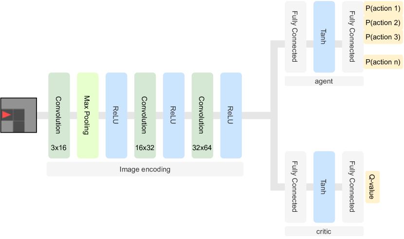
Figure 8: The architecture of the agent A2C model

Figure 8 shows the architecture of our agent. The state observation is encoded using a convolutional neural network (CNN), then passed to the actor-critic network heads composed of two shallow MLPs with one hidden layer each. The Minigrid agent was implemented using the torch-ac implementation presented in the official Minigrid documentation.

We train our agents with the following hyperparameters:

processes $$=20$$

frames $$=1221120$$

batch size $$=256$$

discount factor $$=0.99$$

learning rate $$=3.5\times 10^{-4}$$

PPO hyperparameters:

epochs $$=10$$

lambda coefficient in GAE $$=0.95$$

entropy term coefficient $$=0.01$$

value loss term coefficient $$=0.5$$

maximum norm of the gradient $$=0.5$$

optimizer $$=Adam$$

optimizer epsilon $$=1\times 10^{-8}$$

clipping epsilon for PPO $$=0.2$$

Appendix B Implementation details of the Minigrid Influence Predictors

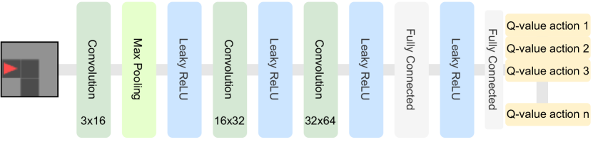
Figure 9: The architecture of the influence predictor network.

Our DQN influence predictors are implemented in Pytorch and all the code is available in our git repository. Figure 9 details the architecture of the influence predictor’s model. We train the influence predictor with the following hyperparameters:

replay buffer capacity $$=50000$$

gamma $$=0.5$$

target update $$=5$$

bootstrap $$=100000$$

batch size $$=64$$

learning rate $$=1\times 10^{-5}$$

optimizer $$=\text{RMSprop}$$

Appendix C Implementations details of Crafter’s Agent and Influence Predictors

As mentioned earlier, both the Agent and the Influence Predictors are implemented using Stable-Baselines3’s [36] PPO [30] implementation. Given the observations are in the form of images, the policy used here ActorCriticCnnPolicy (also from the Stable-Baselines3 [36]).

They use the same values as hyperparameters. The training was done on a single node of a single a40 processor. The training time can be reduced by parallelizing over multiple nodes/processors. The hyperparameters were obtained from [38].

Hyperparameters for the implementations:

nodes $$=1$$

timesteps $$=8994816$$

PPO hyperparameters:

learning rate $$=3\times 10^{-4}$$

Number of steps per env per update $$=4096$$

gamma $$=0.95$$

Number of epochs $$=4$$

batch size $$=128$$

lambda coefficient in GAE $$=0.65$$

entropy term coefficient $$=0.0$$

value loss term coefficient $$=0.5$$

maximum norm of the gradient $$=0.5$$

optimizer $$=Adam$$

clipping parameter $$=0.2$$

Appendix D Experiment 1: Evaluation Survey

In this section, we show a preview of the evaluation survey. Figure 10 shows an example of a prediction task. Then after the participants submit their predictions, they see the correct answer as shown in Figure 11. Afterward, they see one of the three explanation types, Experiential Explanation (Figure 12), Heatmap Explanation (Figure 13), Q-value explanation (Figure 14), or they see no explanation at all. Then they repeat this process two times. After the participants finish the prediction task, they proceed to the reflection survey, where they evaluate their experience with the shown explanations as in figure 15.

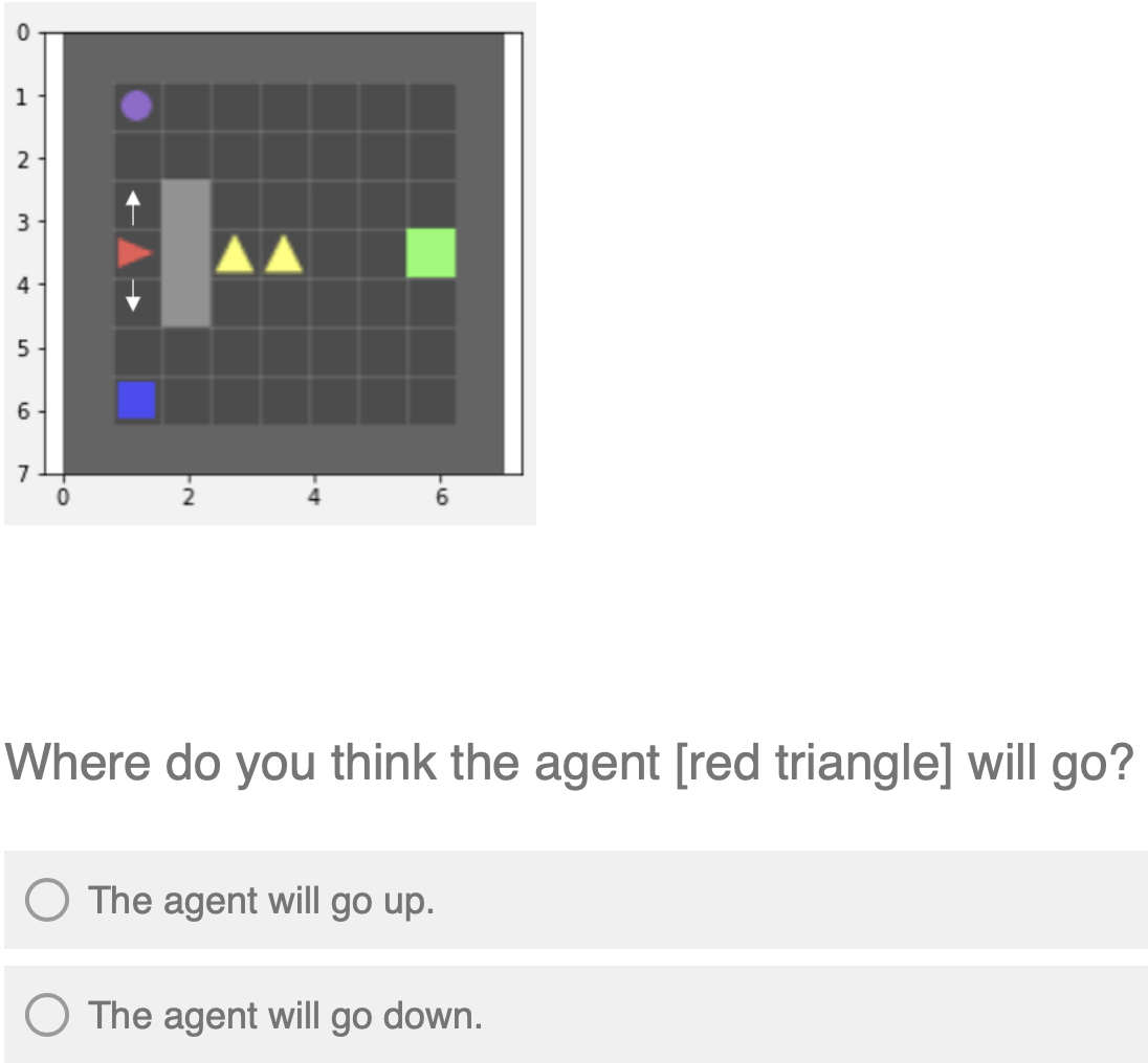
Figure 10: This figure shows an example of the prediction task. The participants saw the map and predicted which direction they thought the agent preferred.

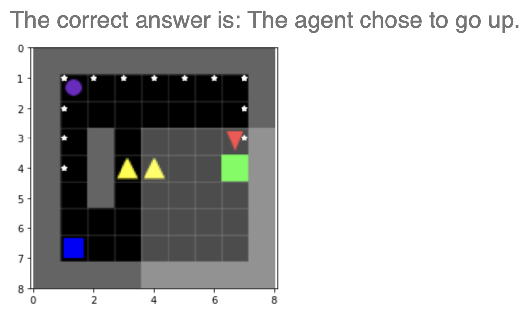
Figure 11: After predicting the agent’s following action, the participants sees the correct actionseeis is the only information provided to the No Explanation group.

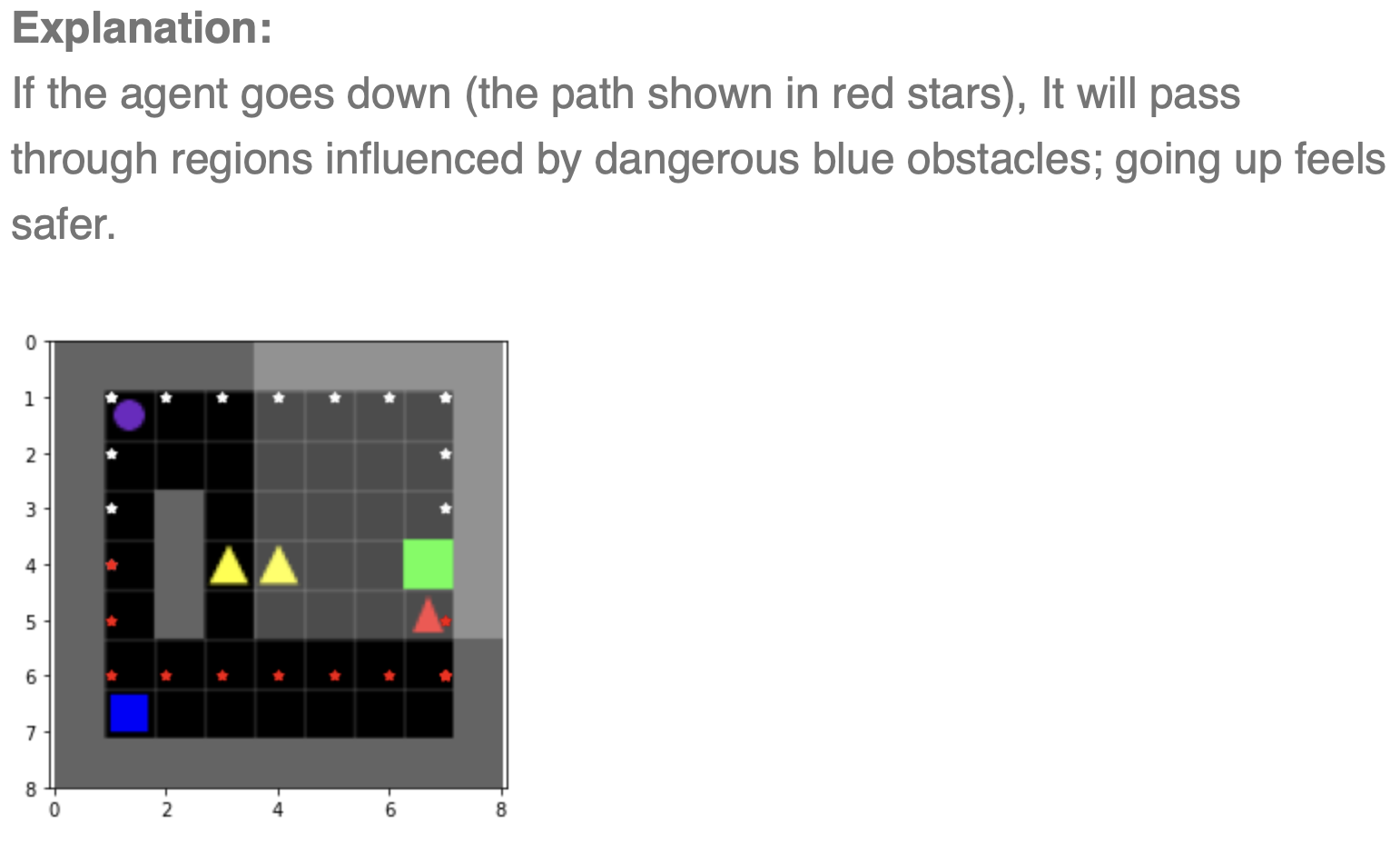
Figure 12: This Experiential Explanation highlights the dangerous objects and compares the agent’s actual and suggested path.

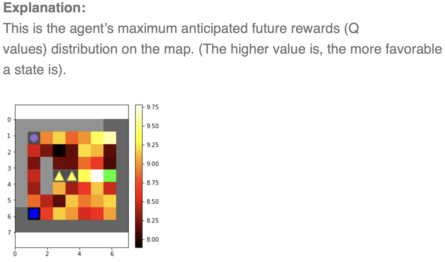
Figure 13: This heat map explanation shows the maximum anticipated future reward for each state in the environment.

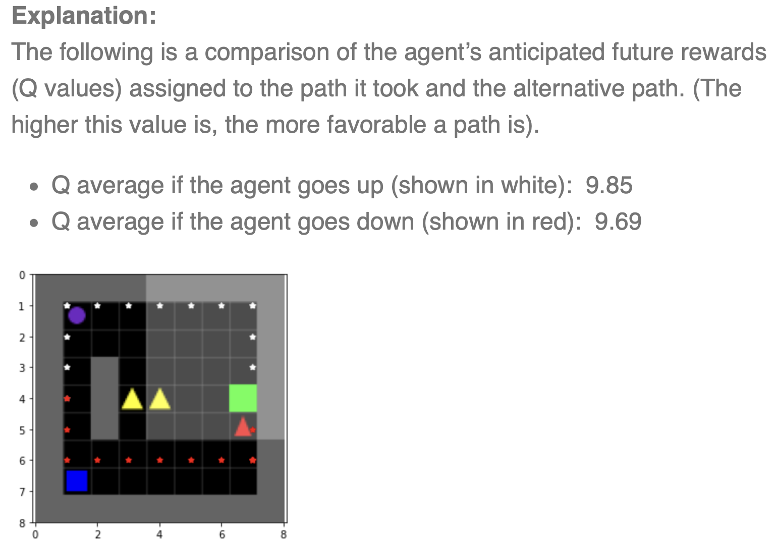
Figure 14: This Q-value explanation compares the actual and suggested paths regarding their average anticipated future reward.

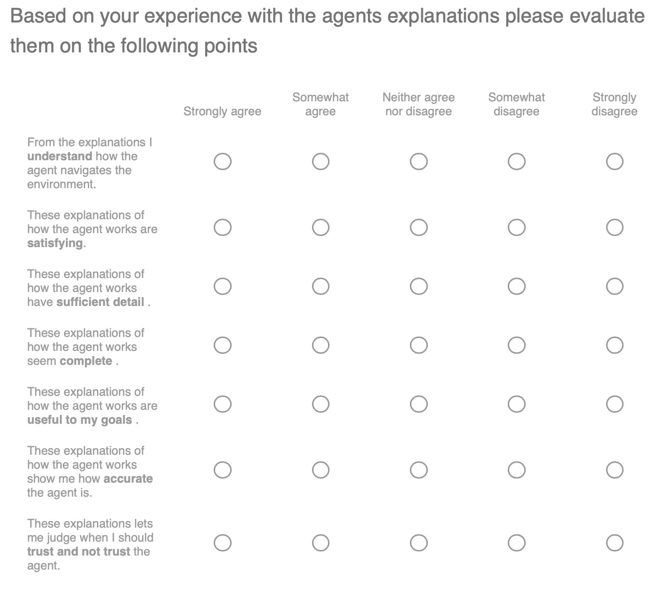
Figure 15: After the experiments, the participants completed the shown satisfaction survey evaluating the explanation type they interacted with on a seven-point scale, measuring helpfulness, satisfaction, understandability, level of detail, completeness, accuracy, and trust.

Appendix E Satisfaction Survey Analysis

Figure 16 shows the results of the satisfaction survey questions shown in 15. The discussion and analysis of the figure 16 results are in the main paper.

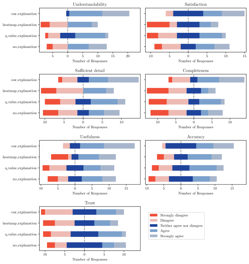
Figure 16: The satisfaction survey results for each explanation quality dimensions grouped by explanation type

Appendix F Crafter Re-skin mappings

Actual Asset	Re-skinned Asset
Materials and Objects
Player (Jade)	No change
Tree	Rock
Grass	No change
Sand	No change
Water	No change
Stone	Scissors
Iron	Paper
Coal	Lizard
Diamond	Electric torch
Zombie	Duck
Table	Parrot
Furnace	Crab
Bridge	No change
Cow	Apple
Inventory Items
Wood	Rock slabs
Wooden pickaxe	Cutter
Wooden sword	Throwing knives
Iron pickaxe	Coaster
Iron sword	Fan
stone pickaxe	Plier
stone sword	Hammer
Parameters
Health	No change
Food	No change
Drink	No change
Energy	No change

Table 4: Original Crafter assets vs their Rock-Paper-Scissors (RPS) asset collection counterparts

Table 4 lists a complete mapping of assets re-skinned assets

References

- \bibcommenthead
- Miller [2019] Miller, T.: Explanation in artificial intelligence: Insights from the social sciences. Artificial intelligence 267, 1–38 (2019)
- Zelvelder et al. [2021] Zelvelder, A.E., Westberg, M., Främling, K.: Assessing explainability in reinforcement learning. In: International Workshop on Explainable, Transparent Autonomous Agents and Multi-Agent Systems, pp. 223–240 (2021). Springer
- Anjomshoae et al. [2019] Anjomshoae, S., Najjar, A., Calvaresi, D., Främling, K.: Explainable Agents and Robots: Results from a Systematic Literature Review. In: Proceedings of the 18th International Conference on Autonomous Agents and MultiAgent Systems. AAMAS ’19, pp. 1078–1088. International Foundation for Autonomous Agents and Multiagent Systems, Richland, SC (2019)
- Alharin et al. [2020] Alharin, A., Doan, T.-N., Sartipi, M.: Reinforcement learning interpretation methods: A survey. IEEE Access 8, 171058–171077 (2020)
- Wells and Bednarz [2021] Wells, L., Bednarz, T.: Explainable AI and Reinforcement Learning—A Systematic Review of Current Approaches and Trends. Frontiers in Artificial Intelligence 4 (2021). Accessed 2022-10-01
- Heuillet et al. [2021] Heuillet, A., Couthouis, F., Díaz-Rodríguez, N.: Explainability in deep reinforcement learning. Knowledge-Based Systems 214, 106685 (2021) https://doi.org/10.1016/j.knosys.2020.106685 . Accessed 2022-09-30
- Puiutta and Veith [2020] Puiutta, E., Veith, E.M.S.P.: Explainable Reinforcement Learning: A Survey. In: Holzinger, A., Kieseberg, P., Tjoa, A.M., Weippl, E. (eds.) Machine Learning and Knowledge Extraction. Lecture Notes in Computer Science, pp. 77–95. Springer, Cham (2020). https://doi.org/10.1007/978-3-030-57321-8_5
- Milani et al. [2023] Milani, S., Topin, N., Veloso, M., Fang, F.: Explainable reinforcement learning: A survey and comparative review. ACM Computing Surveys (2023) https://doi.org/10.1145/3616864
- Chakraborti et al. [2020] Chakraborti, T., Sreedharan, S., Kambhampati, S.: The Emerging Landscape of Explainable Automated Planning & Decision Making. In: Proceedings of the Twenty-Ninth International Joint Conference on Artificial Intelligence, pp. 4803–4811. International Joint Conferences on Artificial Intelligence Organization, Yokohama, Japan (2020). https://doi.org/10.24963/ijcai.2020/669 . https://www.ijcai.org/proceedings/2020/669 Accessed 2022-03-11
- Sutton and Barto [2018] Sutton, R.S., Barto, A.G.: Reinforcement Learning: An Introduction. A Bradford Book, Cambridge, MA, USA (2018)
- Chakraborti et al. [2021] Chakraborti, T., Sreedharan, S., Kambhampati, S.: The emerging landscape of explainable automated planning & decision making. In: Proceedings of the Twenty-Ninth International Conference on International Joint Conferences on Artificial Intelligence, pp. 4803–4811 (2021)
- Ehsan et al. [2019] Ehsan, U., Tambwekar, P., Chan, L., Harrison, B., Riedl, M.O.: Automated rationale generation: a technique for explainable ai and its effects on human perceptions. In: Proceedings of the 24th International Conference on Intelligent User Interfaces, pp. 263–274 (2019)
- Das and Chernova [2020] Das, D., Chernova, S.: Leveraging rationales to improve human task performance. In: Proceedings of the 25th International Conference on Intelligent User Interfaces, pp. 510–518 (2020)
- Juozapaitis et al. [2019] Juozapaitis, Z., Koul, A., Fern, A., Erwig, M., Doshi-Velez, F.: Explainable reinforcement learning via reward decomposition. In: IJCAI/ECAI Workshop on Explainable Artificial Intelligence (2019)
- Anderson et al. [2019] Anderson, A., Dodge, J., Sadarangani, A., Juozapaitis, Z., Newman, E., Irvine, J., Chattopadhyay, S., Fern, A., Burnett, M.: Explaining reinforcement learning to mere mortals: An empirical study. CoRR abs/1903.09708 (2019)
- Septon et al. [2023] Septon, Y., Huber, T., André, E., Amir, O.: Integrating policy summaries with reward decomposition for explaining reinforcement learning agents. In: International Conference on Practical Applications of Agents and Multi-Agent Systems, pp. 320–332 (2023). Springer
- Frost et al. [2022] Frost, J., Watkins, O., Weiner, E., Abbeel, P., Darrell, T., Plummer, B., Saenko, K.: Explaining reinforcement learning policies through counterfactual trajectories. ICML Workshop on Human in the Loop Learning (HILL) (2022)
- van der Waa et al. [2018] Waa, J., Diggelen, J., Bosch, K.v.d., Neerincx, M.: Contrastive explanations for reinforcement learning in terms of expected consequences. arXiv preprint arXiv:1807.08706 (2018)
- Madumal et al. [2020] Madumal, P., Miller, T., Sonenberg, L., Vetere, F.: Explainable reinforcement learning through a causal lens. In: Proceedings of the AAAI Conference on Artificial Intelligence, vol. 34, pp. 2493–2500 (2020)
- Sreedharan et al. [2022] Sreedharan, S., Soni, U., Verma, M., Srivastava, S., Kambhampati, S.: Bridging the gap: Providing post-hoc symbolic explanations for sequential decision-making problems with inscrutable representations. In: International Conference on Learning Representations (2022). https://openreview.net/forum?id=o-1v9hdSult
- Olson et al. [2021] Olson, M.L., Khanna, R., Neal, L., Li, F., Wong, W.-K.: Counterfactual state explanations for reinforcement learning agents via generative deep learning. Artificial Intelligence 295, 103455 (2021)
- Huber et al. [2023] Huber, T., Demmler, M., Mertes, S., Olson, M.L., André, E.: Ganterfactual-rl: Understanding reinforcement learning agents’ strategies through visual counterfactual explanations. In: Proceedings of the 2023 International Conference on Autonomous Agents and Multiagent Systems, pp. 1097–1106 (2023)
- Mnih et al. [2015] Mnih, V., Kavukcuoglu, K., Silver, D., Rusu, A.A., Veness, J., Bellemare, M.G., Graves, A., Riedmiller, M., Fidjeland, A.K., Ostrovski, G., et al.: Human-level control through deep reinforcement learning. nature 518(7540), 529–533 (2015)
- Mnih et al. [2016] Mnih, V., Badia, A.P., Mirza, M., Graves, A., Lillicrap, T., Harley, T., Silver, D., Kavukcuoglu, K.: Asynchronous methods for deep reinforcement learning. In: International Conference on Machine Learning, pp. 1928–1937 (2016). PMLR
- Ng et al. [1999] Ng, A.Y., Harada, D., Russell, S.: Policy invariance under reward transformations: Theory and application to reward shaping. In: Icml, vol. 99, pp. 278–287 (1999). Citeseer
- Hafner et al. [2020] Hafner, D., Lillicrap, T., Norouzi, M., Ba, J.: Mastering atari with discrete world models. arXiv preprint arXiv:2010.02193 (2020)
- Dazeley et al. [2021] Dazeley, R., Vamplew, P., Foale, C., Young, C., Aryal, S., Cruz, F.: Levels of explainable artificial intelligence for human-aligned conversational explanations. Artificial Intelligence 299, 103525 (2021)
- Chevalier-Boisvert et al. [2018] Chevalier-Boisvert, M., Willems, L., Pal, S.: Minimalistic Gridworld Environment for OpenAI Gym. GitHub (2018). https://github.com/maximecb/gym-minigrid
- Willems [2018] Willems, L.: RL Starter Files for MiniGrid (2018). https://github.com/lcswillems/rl-starter-files/tree/4205e05b7905fec16519bc0802596673d86af018 Accessed 2022-09-28
- Schulman et al. [2017] Schulman, J., Wolski, F., Dhariwal, P., Radford, A., Klimov, O.: Proximal policy optimization algorithms. arXiv preprint arXiv:1707.06347 (2017)
- Hoffman et al. [2023] Hoffman, R.R., Mueller, S.T., Klein, G., Litman, J.: Measures for explainable ai: Explanation goodness, user satisfaction, mental models, curiosity, trust, and human-ai performance. Frontiers in Computer Science 5, 1096257 (2023)
- Kiger and Varpio [2020] Kiger, M.E., Varpio, L.: Thematic analysis of qualitative data: Amee guide no. 131. Medical Teacher 42, 846–854 (2020)
- Miles et al. [2020] Miles, M.B., Huberman, A.M., Saldaña, J.: Qualitative Data Analysis : a Methods Sourcebook, Fourth edition edn. SAGE Los Angeles, Los Angeles (2020)
- Zhou et al. [2021] Zhou, J., Gandomi, A.H., Chen, F., Holzinger, A.: Evaluating the quality of machine learning explanations: A survey on methods and metrics. Electronics 10(5), 593 (2021)
- Hafner [2021] Hafner, D.: Benchmarking the spectrum of agent capabilities. arXiv preprint arXiv:2109.06780 (2021)
- Raffin et al. [2021] Raffin, A., Hill, A., Gleave, A., Kanervisto, A., Ernestus, M., Dormann, N.: Stable-baselines3: Reliable reinforcement learning implementations. Journal of Machine Learning Research 22(268), 1–8 (2021)
- Chan et al. [1995] Chan, W.T., Chow, Y.K., Liu, L.F.: Neural network: An alternative to pile driving formulas. Computers and Geotechnics 17(2), 135–156 (1995) https://doi.org/10.1016/0266-352X(95)93866-H
- Stanić et al. [2022] Stanić, A., Tang, Y., Ha, D., Schmidhuber, J.: Learning to Generalize with Object-centric Agents in the Open World Survival Game Crafter (2022)