Policy Learning with New Treatments

Abstract

I study the problem of a decision maker choosing a policy which allocates treatment to a heterogeneous population on the basis of experimental data that includes only a subset of possible treatment values. The effects of new treatments are partially identified by shape restrictions on treatment response. Policies are compared according to the minimax regret criterion, and I show that the empirical analog of the population decision problem has a tractable linear- and integer-programming formulation. I prove the maximum regret of the estimated policy converges to the lowest possible maximum regret at a rate which is the maximum of $N^{-1/2}$ and the rate at which conditional average treatment effects are estimated in the experimental data. I apply my results to design targeted subsidies for electrical grid connections in rural Kenya, and estimate that $97\%$ of the population should be given a treatment not implemented in the experiment.

1 Introduction

Heterogeneous treatment effects are often estimated with a decision problem in mind— should a particular individual be treated? This question has fostered much research in econometrics, statistics, and machine learning. However, relatively less attention has been given to another important margin of the decision— should the treatment itself be adjusted? Whether the treatment is a medical treatment, subsidy, job training, or audit probability, decision makers can usually entertain changing the treatment value that was observed in the data. Even experiments with multivalued treatments may not implement an exhaustive list of treatment values. This is especially true in the social sciences, where testing multiple interventions can be costly, and in the medical sciences, where specific treatment doses are often tested in clinical trials. In this paper I propose a method for allocating treatment to a population when the treatment values themselves can be adjusted to values never before seen in the data. I show how combining the data on existing treatments with economically motivated shape restrictions can be used to design policies that outperform those possible when only previously implemented treatments are considered.

I first formulate a decision problem in which the decision maker observes experimental data on some treatment values and seeks to construct a mapping, or policy, from the space of covariates to the space of treatments in order to maximize some objective function. I assume all experimentation is done before the policy is constructed. This setting, which is common in econometrics, is often referred to as treatment choice or offline policy learning (examples include [1], [3], [15] and other examples mentioned in the literature review thereof, [18], [28], [32], [35], [43], [45]). A distinctive feature of this paper as opposed to most policy learning problems is that the set of treatments that the decision maker can consider may be a strict superset of the support of the treatment random variable observed in the data. This extends policy learning to practically relevant situations in which constraints in the design and implementation of experiments or simply differences in the objectives of the experimenter versus decision maker result in only a few treatment values being piloted in the experiment, while the decision maker may want to consider many more.

Despite the lack of data on the impacts of these never-before-implemented treatments, I show how to bound the response to new treatments using simple, economically interpretable restrictions on the shape of treatment response. For example, a financial incentive may be assumed to have a positive effect, exhibit diminishing returns, or satisfy smoothness conditions. Such shape restrictions are often exploited to partially identify treatment effects (e.g. [23], [29]). The empirical analysis of the present paper demonstrates that such bounds can be adequately informative for choosing whether and how to implement new treatment values. Based on these bounds, I construct a population decision problem to choose which treatment to assign to each covariate value. I use the minimax regret criterion to evaluate treatment choice under partial identification following [22].

As in [20], [15] and the subsequent literature on empirical welfare maximization methods, I propose a decision rule based on solving the empirical analog of the decision problem as a surrogate for the infeasible population objective. The resulting empirical minimax regret estimator is constructed by minimizing maximum regret across an estimate of the partially identified set of treatment response functions. In this way, the resulting policy is robust to model ambiguity induced by introducing new treatments. Despite involving nested, non-closed form optimization problems which characterize the identified set for treatment response, I show how the optimal policy can be computed using the same linear and integer programming tools common in the policy learning literature. The estimator is thus computationally feasible and can be implemented by widely available software.

I show that the proposed decision rule posesses desirable regret properties. The maximum regret obtained under the estimated policy converges to the smallest possible maximum regret that the decision maker could have achieved in the absence of sampling uncertainty– that is, if the population identified set were observed– uniformly across a set of data distributions. The rate at which the regret of the estimated policy converges to its optimum depends on the estimation rate of the response to the treatments which were observed in the data, and hence is an asymptotic rather than finite-sample convergence guarantee. In the case of discrete covariates, or more generally parametric rates of convergence for estimated treatment effects, the rate of convergence of maximum regret is $N^{-1/2}$. Otherwise, maximum regret converges at the nonparametric rate.

I apply the method to data from [17], in which households in rural Kenya were offered one of four prices in $0$, $15$, $25$, or $35$ thousand shillings to connect to the electrical grid. I consider a decision maker able to offer prices in increments of $2.5$ thousand shillings based on household size and income. This represents a much richer set of fifteen possible treatments, allowing for finer targeting of personalized prices to optimize the cost-effectiveness of the subsidy program. To bound the takeup at these new prices, I assume demand is downward sloping and convex. The estimated minimax regret optimal policy assigns prices that were not implemented in the experiment to over $97\%$ of the population, illustrating that constraining the decision maker to treatments that appear in the experimental pilot data can result in suboptimal decisions.

1.a Related Literature

This paper contributes to a growing literature on statistical treatment rules in econometrics beginning with [20] and [15], which introduced the now-common empirical welfare maximization framework. I follow a similar strategy of constructing an empirical analog of the population objective, but seek to minimize the worst-case regret that can occur within the identified set of treatment response.

Forecasting the effects of treatments or policies never before observed in the data is a fundamental goal of econometrics, especially when applied as a guide for public policy (see [9] and [26] for a deep discussion, including a historical overview). Nonetheless, the recent literature on policy learning and treatment choice has generally not considered the introduction of new treatments with partially identified effects. A contemporaneous exception is [27], which studies policies which change the dosage of a vaccine to levels not observed in the data, but does not consider statistical properties of estimated decision rules.

Partial identification has appeared in policy learning and related decision problems in contexts other than consideration of new treatments; examples include [2], [5], [6], [14], [21], [24], [31], [34], [37], and [42], [44]. [2] considers that the effects of new policies may be partially identified when historical data is generated by a deterministic policy, violating the common assumption of strong overlap. [14] studies policy learning when the effect of a binary treatment is partially identified due to unobserved confounding, and proposes algorithms that aim to guarantee improvement relative to a baseline policy. The present work differs not only in that the source of partial identification is new treatments instead of unobserved confounding, but also in that I focus on minimax regret as opposed to regret relative to a baseline. The policy resulting from a minimax regret approach will recommend new treatments more often since the minimax regret criterion considers losses relative to the optimal policy in each state of the world.

[6] studies policy learning with a binary treatment where the conditional average treatment effect is identified up to a rectangular set, meaning it is characterized by bounds which depend only on the covariate value. In contrast, shape restrictions generally yield nonrectangular identified sets. This leads to difficulties when estimating the optimal policy in my setting because the bounds I identify do not in general admit a closed form. However, the extra effort proves valuable in the empirical example of Section 5, where I find that the non-closed form characterization of the identified set using shape restrictions ends up being substantially more informative than pointwise bounds would be for calculating regret.

Many of the previously mentioned works are concerned with binary treatments, while I am concerned with multivalued treatments. [46] and [13] consider policy learning with multivalued treatments and continuous treatments, respectively, but in point-identified settings where all possible treatment values are implemented in the experiment. [42] studies a binary decision between two policies which may not concern the assignment of a binary treatment. Additionally, the new policy may have partially identified effects. The minimax regret rule is derived for a general class of decision rules and applied to the problem of changing the eligibility cutoff for a treatment. The decision problem and assumptions of [42] and the present paper differ, yet the broad goal of choosing amongst new policies with partially identified effects make the two complimentary.

[1] extends policy learning to observational studies where exogeneity of treatment only holds after conditioning on high-dimensional covariates. In contrast, I am motivated by settings in which decision makers have data from a pilot experiment which tested a few treatment values. When this is the case, estimating the effects of policies involving new treatments only requires conditioning on the set of covariates used in the treatment rule, which is typically low-dimensional due to exogenous constraints on the policy class ([15]). [1] also considers infinitesimal, local changes to treatment values; however, I consider new treatments that are sufficiently far from the support of the data as to make local approximations or parametric extrapolations unreliable, necessitating a partial identification approach.

An alternative to the plug-in approach used in this paper and common in policy learning is to average across the parameter space according to some distribution. [5] study optimal decisions in a discrete set under partial identification where Bayes rules and the bootstrap distribution are used to average over the space of identified parameters, while a minimax approach is taken over the partially identified parameters. An important finding is that plug-in-rules may be dominated in the asymptotic limit experiment. See [10] and [11] for further discussion of asymptotic optimality of statistical treatment rules.

The rest of the article is organized as follows: Section 2 describes the decision problem in the population and shows how to incorporate information from shape restrictions. Section 3 describes the empirical minimax regret problem and the algorithm for estimating the optimal policy. Section 4 describes the convergence guarantees. Section 5 applies the method to study personalized subsidies to connect to the electrical grid in rural Kenya.

2 Population Decision Problem

2.a General Framework

A decision maker has access to experimental data and must choose a rule assigning individuals to treatments based on their observable covariates. The experimental data is described by random variables $(D,X,Y)$ taking values in $\mathcal{D}_{0}\times\mathcal{X}\times\mathcal{Y}$ where $D$ is a randomly assigned treatment, $X$ are observed covariates, and $Y$ is an outcome of interest. Although the random variable $D$ only takes values in $\mathcal{D}_{0}$, the decision maker can consider assigning individuals to any treatment value $d\in\mathcal{D}$ where $\mathcal{D}$ is potentially larger than $\mathcal{D}_{0}$. Hence, I assume the existence of potential outcomes $Y(d)$ for all $d\in\mathcal{D}$. The set $\mathcal{D}$ has cardinality $|\mathcal{D}|=J<\infty$, and its elements are denoted by $d_{j}$ for $j\in\{1,\dots,J\}$. The observed outcome $Y$ is generated as $Y=Y(D)$. Let $P$ denote the distribution of $(D,X,(Y(d))_{d\in\mathcal{D}})$. The decision maker seeks a policy $\pi\mathrel{\mathop{\mathchar 58\relax}}\mathcal{X}\mapsto\mathcal{D}$ which assigns individuals to treatment status based on their observable covariates. The policy is chosen from some set $\Pi$ which is taken as given. The treatment assigned to an individual with covariate values $X$ is $\pi(X)$ and the realized outcome is $Y(\pi(X))$. The decision maker has some utility function $u(d,x,y)$ which may depend on the treatment assigned, covariates, and the realized outcome of interest. I assume the decision maker is utilitarian and ultimately cares about the expected utility derived from the data realized from the policy, resulting in the following problem that the decision maker would like to solve

$$\max_{\pi\in\Pi}\mathbb{E}_{P}\bigg{[}u(\pi(X),X,Y(\pi(X)))\bigg{]}$$

$$=\max_{\pi\in\Pi}\mathbb{E}_{P}\bigg{[}v_{P}(\pi(X),X)\bigg{]}$$

where $v_{P}(d,x)\mathrel{\mathop{\mathchar 58\relax}}=\mathbb{E}_{P}[u(d,X,Y(d))\mid X=x]$ is the conditional mean utility.

Two sources of ignorance on the decision maker’s part make this problem infeasible to solve in practice. The first is that only a sample is observed, so the population probability distribution is unknown. The second is that even if the population distribution of the data $(D,X,Y)$ were known, the effects of some treatments are not identified because they are never observed. In particular, the function $v$ depends on the distribution of potential outcomes $Y(d)$ for values of $d$ not in $\mathcal{D}_{0}$. Since data on these potential outcomes are not observed in the sample, the decision maker’s objective is not point identified. To deal with partial identification, I will solve a proxy problem which is robust to partial identification in that it achieves uniformly low regret across the identified set for $v$. Since only sample data is available, I solve the empirical or plug-in version of this problem.

Following [20] and much of the econometric literature on treatment choice, policies will be evaluated based on their expected regret. For a chosen policy $\pi$, the regret of $\pi$ is the difference in expected utility obtained from implementing the first-best policy versus $\pi$. The first-best policy maps each covariate value $x$ to $\arg\max_{d}v_{P}(d,x)$. For any chosen policy $\pi$, the expected regret of implementing $\pi$ versus implementing the first-best policy is

$$R_{P}(\pi) \mathrel{\mathop{\mathchar 58\relax}}=\mathbb{E}_{P}\bigg{[}\max_{d}v_{P}(d,X)-v_{P}(\pi(X),X)\bigg{]}$$

Since $v_{P}$ is not identified, regret is not identified either. However, letting $\mathcal{V}_{P}$ be the as-of-yet-uncharacterized identified set for $v_{P}$ determined by the experimental data, the maximum expected regret that can occur if the decision maker implements policy $\pi$ is given by

$$\overline{R}_{P}(\pi)\mathrel{\mathop{\mathchar 58\relax}}=\max_{v\in\mathcal{V}_{P}}\mathbb{E}_{P}\bigg{[}\max_{d\in\mathcal{D}}v(d,X)-v(\pi(X),X)\bigg{]}$$

I use the minimax regret criterion to guide the choice of policy. This means $\pi$ is chosen to minimize the largest regret that can occur within the identified set— that is, $\overline{R}_{P}(\pi)$. Therefore, the decision maker chooses $\pi$ to minimize the worst-case expected regret as follows

$$\pi_{P}^{*}\in\arg\min_{\pi\in\Pi}\overline{R}_{P}(\pi)=\arg\min_{\pi\in\Pi}\max_{v\in\mathcal{V}_{P}}\mathbb{E}_{P}\bigg{[}\max_{d\in\mathcal{D}}v(d,X)-v(\pi(X),X)\bigg{]}$$ (1)

This ensures that the chosen policy minimizes regret uniformly across the identified set. If the minimizer is not unique, the decision maker is indifferent among them.

The minimax regret criterion is not the only method for comparing statistical decisions with partially identified effects. In the context of treatment choice, [25] compares the minimax regret criterion with the maximin welfare and subjective expected welfare criteria, two common alternatives. Under the maximin welfare criterion, the decision maker seeks to maximize the minimum possible level of the outcome that could be attained as opposed to the minimum gap between the attained and first-best level of the outcome. The method for construction and estimation of the optimal policy that follows can be applied when using the maximin welfare criterion as well. Indeed, it can be obtained as a simplification of what follows by replacing $\max_{d\in\mathcal{D}}v(d,X)$ with $0$ in (1). However, the resulting estimator will of course have different behavior and regret properties.

In some settings the maximin criterion can be quite conservative (see the discussion of [41] found in [36]). Indeed, unless a new treatment $d\in\mathcal{D}\setminus\mathcal{D}_{0}$ can be guaranteed to outperform the original set of treatments in every possible state of the world $v\in\mathcal{V}_{P}$, the maximin welfare criterion will not implement new treatments. This is because under the maximin welfare criterion the decision is driven entirely by hedging against the least favorable state of the world. In contrast, the minimax regret criterion considers the suboptimality gap in all possible states of the world. The decision maker measures the performance of the policy in each state of the world according to the benchmark of optimality in that state of the world. I follow [22] in applying the minimax regret criterion to treatment choice. This represents a particular choice of loss function and in turn delivers a point estimate of an optimal policy.

When the probability of each state of the world $v\in\mathcal{V}_{P}$ can be described by a probability distribution, the Bayesian approach to decision making can be applied. This consists of setting a prior over states of the world $v\in\mathcal{V}_{P}$, using the data to form a posterior, and selecting a treatment policy which maximizes posterior expected welfare. One potential weakness of this approach in the context of introducing new treatments is that the lack of identification means that even in large samples, the influence of the prior on the posterior will be substantial. Yet another possible approach to estimate the effects of treatments that lie outside the support of the data could be to extrapolate using a parametric model, thus circumventing entirely the need for partial identification. However, when the new treatments are sufficiently far from the support of the data, a parametric point-identified model substantially understates the degree of model uncertainty. This is illustrated in Section 5 where the differences between parameter values within the identified set are economically significant.

2.b Imposing Shape Restrictions

I now describe how a tractable characterization of the minimax regret problem (1) can be obtained using shape restrictions on the treatment response. Assume that utility is linear in the outcome of interest so $u(d,x,y)=b(d,x)y-c(d,x)$ for known functions $b$ and $c$. While it is often possible to avoid the assumption of linear utility by simply redefining $Y$ as utility, in some applications (such as in Section 5) it may be more natural to impose shape restrictions in terms of the original outcome variable, which may relate to a structural economic quantity such as a demand curve. In Section 5, $y$ will be a purchase indicator, $b(d,x)$ will be the amount of the subsidy, and $c(d,x)$ represents fixed costs of treatment, which I take to be $0$. Note that the assumption of linearity implies $v_{P}(d,x)=b(d,x)m_{P}(d,x)-c(d,x)$ where $m_{P}(d,x)\mathrel{\mathop{\mathchar 58\relax}}=\mathbb{E}_{P}[Y(d)\mid X=x]$ is the conditional mean response function. Moreover, any alternative conditional mean response $m$ induces an alternative expected utility function. I therefore will also use the notation $v_{m}(d,x)\mathrel{\mathop{\mathchar 58\relax}}=b(d,x)m(d,x)-c(d,x)$ where conditional mean utilities are indexed by conditional mean response functions rather than probability distributions. Since $b$ and $c$ are known functions, in order to characterize maximum regret it is sufficient to characterize the identified set for $m_{P}$.

The decision maker has experimental data on the effectiveness of some treatments. This means that $m_{P}(d,\cdot)$ is identified for every $d\in\mathcal{D}_{0}$. For this information on the effects of treatments in $\mathcal{D}_{0}$ to be informative about the effects of treatments in $\mathcal{D}\setminus\mathcal{D}_{0}$, some structure must be known about the mean conditional response function $m_{P}$. For example, the decision maker may know that demand is downward sloping, that a particular intervention features decreasing returns to scale, or that the treatment response exhibits some smoothness properties. By combining knowledge of $m_{P}(d,\cdot)$ for $d\in\mathcal{D}_{0}$ with such shape restrictions, the effects of new treatments may be partially identified.

Let the set of shape-restricted mean conditional response functions be denoted $\mathcal{S}$, so that it is assumed ex ante that $m_{P}\in\mathcal{S}$. Then the sharp identified set for $m_{P}$ is simply

$$\mathcal{M}_{P} \mathrel{\mathop{\mathchar 58\relax}}=\mathcal{S}\cap\{m\mathrel{\mathop{\mathchar 58\relax}}m(d,X)=m_{P}(d,X),\;P-\text{a.s.},\;\forall d\in\mathcal{D}_{0}\}$$

which represents the set of functions which obey the shape restrictions and match identified population means. A useful structure that $\mathcal{S}$ is assumed to possess is that a hypothetical conditional mean response function $m$ is in $\mathcal{S}$ if and only if $m(\cdot,X)$ satisfies some shape restrictions almost surely. That is, $\mathcal{S}$ encapsulates assumptions about the shape of $m_{P}$ across $d$ for fixed $x$, leaving the behavior of $m_{P}$ across $x$ unrestricted ([19], [21]). This means that an individual at a particular covariate value is assumed to have an expected treatment response that is decreasing, convex, smooth, etc. Hence, the maximization over $v$ (equivalently maximization over $m\in\mathcal{M}_{P}$) in (1) is solved by considering each value of $x$ in isolation and finding the $m(\cdot,x)$ which maximizes regret. This allows the maximum to be interchanged with the expectation in the minimax regret problem (1)

$$\min_{\pi\in\Pi}\max_{m\in\mathcal{M}_{P}} \;\mathbb{E}_{P}\bigg{[}\max_{d\in\mathcal{D}}v_{m}(d,X)-v_{m}(\pi(X),X)\bigg{]}$$

$$=\min_{\pi\in\Pi} \;\mathbb{E}_{P}\bigg{[}\max_{m\in\mathcal{M}_{P}}\bigg{(}\max_{d\in\mathcal{D}}v_{m}(d,X)-v_{m}(\pi(X),X)\bigg{)}\bigg{]}$$

$$=\min_{\pi\in\Pi} \;\mathbb{E}_{P}\bigg{[}\sum_{j=1}^{J}\pi_{j}(X)\Gamma_{j,P}(X)\bigg{]}$$ (2)

where $\pi_{j}(X)=\mathbbm{1}[\pi(X)=d_{j}]$ and

$$\Gamma_{j,P}(X)\mathrel{\mathop{\mathchar 58\relax}}=\max_{m\in\mathcal{M}_{P}}\bigg{(}\max_{d\in\mathcal{D}}v_{m}(d,X)-v_{m}(d_{j},X)\bigg{)}$$

which can be interpreted as the contribution to maximum expected regret of assigning a person with covariate values $X$ to treatment $d_{j}$.

The optimization problem (2.b) defines the policy which is optimal in terms of its population minimax regret. The benefit of imposing shape restrictions only on the behavior of $m_{P}$ across $d$ is that the representation (2.b) is an optimization problem over a population expected loss defined by $\Gamma_{j,P}(X)$. This problem possesses a form similar to decision problems presented in [1], [6], and others, with the key distinction that the covariate-level loss $\Gamma_{j,P}(X)$ is itself the solution to an optimization problem which generally will not have a closed-form solution. Nonetheless, the minimax regret problem (2.b) can be cast in terms of the empirical welfare maximization framework of [15]. In the following section, I discuss how to set up the empirical analog of the nested optimization problem (2.b) and provide a computationally attractive algorithm for solving it.

3 Estimation

The optimization problem (2.b) is infeasible for the decision maker because in practice only a sample
$\{(D_{i},X_{i},Y_{i})\}_{i=1}^{N}$ is observed. Instead, I propose solving the empirical analog of (2.b) to obtain an estimate of the population optimal policy. Insofar as the constraints of this problem are constructed from consistent estimators, the optimal policy will inherit similar properties.

In this section I describe the empirical analog of (2.b) and provide a solution procedure. It consists of first estimating the effects of the treatments which were implemented in the experimental data, then constructing estimates of $\Gamma_{j,P}(X_{i})$ for every observation $i$ and treatment $j$, and finally plugging these estimates into the empirical analog of (2.b) where the sample mean is used instead of the population expectation. I show how $\Gamma_{j,P}(X_{i})$ can be expressed using linear programming, resulting in a mixed integer-linear programming formulation for (2.b) for many policy classes $\Pi$.

First, I estimate the mean conditional response function for every $d\in\mathcal{D}_{0}$, denoted $\hat{m}_{0}(d,x)$. Except for high level conditions on the accuracy of the estimate detailed in Section 4, I remain agnostic about the how the estimate is constructed. The estimate $\hat{m}_{0}$ is used to construct an estimate of the identified set for $m_{P}(\cdot,X_{i})$ for each $i$ as a function of $d$ in all of $\mathcal{D}$, which represents covariate-level bounds on the effects of new treatments. The empirical analog of $\mathcal{M}_{P}$ is the set of functions which obey the shape restrictions and match estimated sample means, and is denoted by $\hat{\mathcal{M}}\mathrel{\mathop{\mathchar 58\relax}}=\mathcal{S}\cap\{m\mathrel{\mathop{\mathchar 58\relax}}m(d,X_{i})=\hat{m}_{0}(d,X_{i})\;\forall i,\;\forall d\in\mathcal{D}_{0}\}$. I assume it is nonempty. As discussed in Section 4, estimators which violate the shape restrictions and hence yield an empty $\hat{\mathcal{M}}$ can be projected onto the set of functions which satisfy the shape restrictions. Since these are assumed to hold in the population, imposing such shape restrictions on estimators typically improves performance in finite samples ([4]).

This is then used to construct estimates $\hat{\Gamma}_{j}(X_{i})$ of the covariate-level loss $\Gamma_{j,P}(X_{i})$, for every observation $i$ and treatment $j$. That is,

$$\hat{\Gamma}_{j}(X_{i})=\max_{m\in\hat{\mathcal{M}}}\bigg{(}\max_{d\in\mathcal{D}}v_{m}(d,X_{i})-v_{m}(d_{j},X_{i})\bigg{)}$$ (3)

These estimates are then used in the program

$$\hat{\pi}\mathrel{\mathop{\mathchar 58\relax}}=\arg\min_{\pi\in\Pi}\sum_{i=1}^{n}\sum_{j=1}^{J}\pi_{ij}\hat{\Gamma}_{j}(X_{i})$$ (4)

where $\pi_{ij}=\mathbbm{1}[\pi(X_{i})=d_{j}]$.

Having defined the estimator for the minimax regret optimal policy (4), I turn to computationally convenient methods for estimating $\hat{\Gamma}_{j}(X_{i})$ and thereby the policy $\hat{\pi}$. This is achieved by expressing $\hat{\Gamma}_{j}(X_{i})$ through linear programs and considering policy classes $\Pi$ which can be expressed using linear and integer constraints. In doing so, I impose some additional structure on the set of shape restricted functions $\mathcal{S}$. Specifically, I assume the a priori knowledge on shape restrictions can be summarized through linear transformations of the treatment response vector for almost every $x$.

Assumption 3.1.

There exists some matrix $S$ and some vector $r$ such that the conditional mean response function $m(d,x)$ is in the set $\mathcal{S}$ if and only if $Sm(\cdot,X)\leq r$ $P-$almost surely, where $m(\cdot,x)\mathrel{\mathop{\mathchar 58\relax}}=(m(d_{1},x),\dots,m(d_{J},x))^{\prime}$.

This assumption is quite flexible in the class of shape restrictions it can handle. For example, restrictions on the first, second, or higher differences of the mean conditional response can be expressed this way, allowing for $m_{P}$ to be constrained to be decreasing, Lipschitz, convex, or obey higher order smoothness conditions ([29]). Upper and lower bounds on $m_{P}$ can also be expressed through such constraints. Appendix B describes in detail how the restrictions of decreasing demand and diminishing returns to the subsidy are applied to the empirical example in Section 5. The following example conveys the practical use of the assumption.

Example 3.2.

Suppose $\mathcal{D}=\{1,2,3,4\}$ and $m_{P}(d,x)$ is assumed to be increasing and concave in $d$. Then $m\in\mathcal{S}$ if and only if $Sm(\cdot,X)\leq r$ $P$-almost surely where

$$S=\begin{bmatrix}1&-1&0&0\\ 0&1&-1&0\\ 0&0&1&-1\\ 1&-2&1&0\\ 0&1&-2&1\\ \end{bmatrix}\quad\quad r=\begin{bmatrix}0\\ 0\\ 0\\ 0\\ 0\end{bmatrix}$$

Here the first three rows of $S$ ensure that $m$ is increasing, and the second two rows of $S$ ensure concavity.

To ensure that $\hat{\mathcal{M}}$ consists of functions which match sample analogs of identified means on $\mathcal{D}_{0}$, I introduce the $|\mathcal{D}_{0}|\times J$ matrix $F$ where $F_{kj}=1$ if $d_{j}$ is the $k$th element of $\mathcal{D}_{0}$ and $F_{kj}=0$ otherwise. Then the identified set $\mathcal{M}_{P}$ is the set of all $m$ such that $Sm(\cdot,X)\leq r$ and $Fm(\cdot,X)=m_{0,P}(\cdot,X)$ almost surely, where $m_{0,P}(\cdot,X)=(m_{P}(d,X))_{d\in\mathcal{D}_{0}}$. That is,

$$\mathcal{M}_{P} =\{m\mathrel{\mathop{\mathchar 58\relax}}Sm(\cdot,X)\leq r,\;Fm(\cdot,X)=m_{0,P}(\cdot,X),\;P-\text{a.s.}\}$$

which allows the empirical analog $\hat{\mathcal{M}}$ to be expressed as

$$\hat{\mathcal{M}} =\{m\mathrel{\mathop{\mathchar 58\relax}}Sm(\cdot,X_{i})\leq r\;\forall i,Fm(\cdot,X_{i})=\hat{m}_{0}(\cdot,X_{i})\;\forall i\}$$

where $\hat{m}_{0}(\cdot,x)^{\prime}=(\hat{m}_{0}(d,x))_{d\in\mathcal{D}_{0}}$. By expressing $\hat{\mathcal{M}}$ this way it is possible to express $\hat{\Gamma}_{j}(X_{i})$ as the maximum of $J$ linear programs. Define the estimate

$$\hat{\Gamma}_{jk}(X_{i})\mathrel{\mathop{\mathchar 58\relax}}=\max_{m\in\hat{\mathcal{M}}}v_{m}(d_{k},X_{i})-v_{m}(d_{j},X_{i})$$

which measures the contribution to expected regret of assigning an individual $d_{j}$ instead of assigning them $d_{k}$, conditional on $X_{i}$. For each observation $i$ and treatments $j$ and $k$, construct $b_{jk}(X_{i})$ as a vector in $\mathbbm{R}^{J}$ with $b(d_{k},X_{i})$ in the $k^{th}$ entry and $b(d_{j},X_{i})$ in the $j^{th}$ entry, and zeros everywhere else. Construct $c_{jk}(X_{i})$ likewise. Then

$$\begin{split}\hat{\Gamma}_{jk}(X_{i})=\max_{m}\quad b_{jk}(X_{i})^{\prime}m-&c_{jk}(X_{i})\\ s.t.\quad Sm&\leq r\\ Fm&=\hat{m}_{0}(\cdot,X_{i})\end{split}$$ (5)

where the choice variable $m$ is a vector in $\mathbbm{R}^{J}$. After defining $\hat{\Gamma}_{j}(X_{i})=\max_{k}\hat{\Gamma}_{jk}(X_{i})$, these estimates can be used in the program (4).

Despite the linear programming representation of $\hat{\Gamma}_{jk}(X_{i})$, computing $\hat{\Gamma}_{j}(X_{i})$ for all $i$ and $j$ appears to require $NJ^{2}$ linear programs total (one for each $i$, $j$, and $k$ combination). However, a dual formulation detailed in Appendix B demonstrates that $\max_{k}\hat{\Gamma}_{jk}(X_{i})$ can be computed with a single linear program, reducing this burden to $NJ$ linear programs; moreover holding $j$ fixed the linear programs for all observations can be stacked together and solved simultaneously. This reduces the computational burden to only $J$ programs, one for each possible treatment in $\mathcal{D}$. Additionally, in the case of discrete covariates, it is only necessary to construct $\hat{\Gamma}_{j}(X_{i})$ for unique values of $X_{i}$, which may be substantially smaller than the sample size $N$.

Having computed the covariate-level loss estimates $\hat{\Gamma}_{j}(X_{i})$ that appears in (4), optimization of the policy $\pi$ over the set $\Pi$ can be performed according to established methods in policy learning. In many cases, $\Pi$ can be represented by linear and integer constraints. Examples include linear eligibility scores, decision trees, and treatment sets with piecewise linear boundaries ([15], [28], [46]). When this is the case, the problem (4) is a mixed integer-linear program for which highly optimized solvers are readily available. In Section 5, I use a class of linear eligibility score policies, which is described using linear and integer constraints in Appendix B.

Since optimization of $\pi$ using mixed integer-linear programming is standard practice in policy learning problems, the only additional computational burden resulting from considering new treatments is the $J$ linear programs mentioned above. For the example in Section 5 I found the computation time for $\hat{\Gamma}_{j}(X_{i})$ to be at most a similar order of magnitude as that of the estimation $\hat{\pi}$ and sometimes much shorter, depending on the complexity of the policy class. For the baseline specification in Section 5 this resulted in a total runtime of a few hours. Constructing $\hat{\Gamma}_{j}(X_{i})$ can often benefit from parallelization so that the overall computational burden is not much larger than the point identified case.

4 Regret Convergence

In this section I investigate theoretical guarantees on the performance of the estimated policy $\hat{\pi}$. Following [20], I evaluate the performance of policies in terms of their statistical regret. In particular, I show that the regret of the estimated policy $\hat{\pi}$ converges to the lowest possible maximum regret the decision maker could achieve if the population identified set under distribution $P$ were observed, uniformly across $P$. Specifically, the regret guarantees will be of the form

$$\sup_{P}\left(\mathbb{E}_{P}[\overline{R}_{P}(\hat{\pi})]-\overline{R}_{P}(\pi^{*}_{P})\right)\leq\mathcal{O}(N^{-1/2}\vee\rho_{N}^{-1})$$

where $P$ ranges across an appropriate set defined below, implying that

$$\sup_{P}\mathbb{E}_{P}[\overline{R}_{P}(\hat{\pi})]\leq\sup_{P}\overline{R}_{P}(\pi^{*}_{P})+\mathcal{O}(N^{-1/2}\vee\rho_{N}^{-1})$$

for an appropriate sequence $\rho_{N}^{-1}\to 0$. Since the estimated policy $\hat{\pi}$ is constructed using consistent estimates of the partially identified set, these guarantees will generally be asymptotic in nature. Above, the expectation only averages across realizations of the estimator $\hat{\pi}$ because $\overline{R}_{P}(\cdot)$ is defined using the population probability measure $P$. The interpretation of this bound is that asymptotically the performance of the estimated policy $\hat{\pi}$ as measured by its maximum regret across distributions $P$ (and the identified set under $P$) apporaches the performance of the population optimal policy $\pi^{*}_{P}$.

Note that $0\leq\overline{R}_{P}(\pi^{*}_{P})\leq\overline{R}_{P}(\hat{\pi})$ so that, averaging across realizations of the estimate $\hat{\pi}$, the worst-case expected regret of $\hat{\pi}$ is growing arbitrarily close to $\overline{R}_{P}(\pi^{*}_{P})$, the lowest possible maximum regret the decision maker could achieve in the absence of sampling uncertainty. Moreover, in general no policy $\pi$ can achieve zero maximum regret across the entire identified set, resulting in $\overline{R}_{P}(\pi^{*}_{P})\geq 0$ typically holding with strict inequality for the population optimal $\pi^{*}_{P}$.

I now discuss assumptions sufficient for such guarantees. The main assumptions on the joint distribution of the data are random assignment of treatment and boundedness of the components of utility.

Assumption 4.1.

$\{(Y_{i},D_{i},X_{i})\}_{i=1}^{n}$ are iid copies of $(Y,D,X)$, generated by $P$ which satisfies

1. $D\perp Y(d)\mid X$ for all $d\in\mathcal{D}$

2. There exists $C<\infty$ such that $m_{P}(d,X)$, $b(d,X)$, and $c(d,X)$ are all bounded in absolute value by $C$ almost surely, for each $d\in\mathcal{D}$

Assumption 4.1.1 reflects the standard exogeneity condition that holds in the randomized experiment settings I use as a motivating example. It may also hold in observational studies, in which case it may be a strong assumption. In many randomized experiments the stronger condition $D\perp(Y(d),X)$ is satisfied. When this is true, it is sufficient to estimate $m_{P}(d,x)=\mathbb{E}_{P}[Y(d)\mid\tilde{X}=x]$, where $\tilde{X}$ is a subset of covariates $X$ which directly enter the policy. $\tilde{X}$ may be of a much lower dimension than $X$ since policies are often restricted to be relatively simple ([15]). In Section 5, there are two covariates which enter the policy. Henceforth, I do not distinguish between the covariates required for Assumption 4.1.1 and the covariates used for the policy. Assumption 4.1.2 restricts decision maker preferences and the expectation of the random variable $Y$. In the example of Section 5 the outcome $Y$ is bounded while $b(d,x)$ is constant in $x$ and $c(d,x)=0$, satisfying this condition trivially.

The estimate $\hat{m}$ also must be sufficiently accurate in the following sense

Assumption 4.2.

For some sequence $\rho_{N}\to\infty$ and some class of distributions $\mathcal{P}$, the estimate $\hat{m}$ satisfies

1. $\lim\sup_{N\to\infty}\sup_{P\in\mathcal{P}}\rho_{N}\mathbb{E}_{P}\bigg{[}\frac{1}{N}\sum_{i=1}^{N}\lVert\hat{m}_{0}(\cdot,X_{i})-m_{0,P}(\cdot,X_{i})\rVert\bigg{]}<\infty$

2. $\hat{\mathcal{M}}=\{m\mathrel{\mathop{\mathchar 58\relax}}Sm(\cdot,X)\leq r,\;Fm(\cdot,X)=\hat{m}_{0}(\cdot,X)\}$ is nonempty, almost surely, for all $P\in\mathcal{P}$.

One common setting in which Assumption 4.2.1 holds with $\rho_{N}=N^{1/2}$ is when the covariates are discrete and sample averages may be used. Alternatively, $m_{P}(d,\cdot)$ may be assumed to belong to a parametric family, for each value of $d\in\mathcal{D}_{0}$. Since $m_{P}(d,\cdot)$ is identified holding $d\in\mathcal{D}_{0}$ fixed, parametric assumptions on the relationship between covariates and the outcome of interest conditional on treatment values observed in the data may be weaker assumptions than the kinds of parametric assumptions that would allow one to extrapolate to new treatments. [15] provides more general conditions under which Assumption 4.2.1 is satisfied when $\hat{m}$ is constructed via local polynomial regression.

Assumption 4.2.2 is not a restrictive assumption. Unless $m_{P}$ is on the boundary of $\mathcal{S}$, the estimated set $\hat{\mathcal{M}}$ will typically be nonempty with high probability as $N$ grows even if 4.2.2 is not assumed. In finite samples, an estimator that yields an empty $\hat{\mathcal{M}}$ can be projected onto the set of all $\hat{m}$ such that $\hat{\mathcal{M}}$ is nonempty. Since $\hat{m}_{0}(\cdot,X)$ is a vector in $\mathbbm{R}^{|\mathcal{D}_{0}|}$ and $\mathcal{S}$ is described by linear inequalities, this is a simple convex minimum norm problem that can be solved by quadratic programming.

Finally, the choice set $\Pi$ is assumed to satisfy a standard condition on its complexity.

Assumption 4.3.

For each $d\in\mathcal{D}$, the class of sets $\{x\mathrel{\mathop{\mathchar 58\relax}}\pi(x)=d,\;\pi\in\Pi\}$ is a VC-class of sets with VC dimension at most $\mathbf{v}<\infty$.

For a formal definition of the VC dimension, see [39]. The assumption of finite VC dimension limits the complexity of the class $\Pi$; specifically, Assumption 4.3 ensures that $\Pi$ cannot be so flexible as to assign any arbitrary subset of a collection of $\mathbf{v}+1$ points in $\mathcal{X}$ to treatment $d$. This assumption is commonly invoked in offline policy learning settings as a way to express the constraints faced by decision makers ([15]); this may be for the sake of interpretation, fairness, ease of implementation, political constraints, etc. The types of rules discussed in Section 3 which can be expressed using linear and integer constraints, like linear eligibility scores and decision trees, satisfy this assumption under bounds on the number of inputs to the eligibility score or the depth of the decision tree. The assumption of VC dimension also plays an important role in the convergence of the regret of the optimal policy by ensuring the policy does not overfit the sample data. This assumption can be relaxed by instead using a holdout validation sample which acts as a regularizer in the estimation of the policy ([28]).

Under these assumptions, the following regret bound is obtained:

Theorem 4.4.

Let $\mathcal{P}_{C}$ be a set of distributions for which (1) Assumptions 4.1 holds with constant $C$ and (2) Assumption 4.2 holds. Under Assumptions 3.1 and 4.3,

$$\sup_{P\in\mathcal{P}_{C}}\left(\mathbb{E}_{P}[\overline{R}_{P}(\hat{\pi})]-\overline{R}_{P}(\pi^{*}_{P})\right)\leq\mathcal{O}(N^{-1/2}\vee\rho_{N}^{-1})$$

is satisfied. As a result,

$$\sup_{P\in\mathcal{P}_{C}}\mathbb{E}_{P}[\overline{R}_{P}(\hat{\pi})]\leq\sup_{P\in\mathcal{P}_{C}}\overline{R}_{P}(\pi^{*}_{P})+\mathcal{O}(N^{-1/2}\vee\rho_{N}^{-1})$$ (6)

The rate of convergence of the maximum regret is the slower of two rates: $N^{-1/2}$, and the estimation rate of $\hat{m}_{0}$ in Assumption 4.2. This first rate is driven by the convergence of an empirical process uniformly over the policy class, which is $N^{-1/2}$ under Assumption 4.3 ([39]). The second rate reflects that the regret of the estimated policy depends on the behavior of the linear program (5), the constraints of which depend on identified moments of the data and must be estimated. In turn, the value of the linear program can be shown to converge to its population counterpart at the same rate as the constraints (see [12] and [33], related results in econometrics include [7], [8]). Because Assumption 4.2 is only a condition on the rate of convergence of this estimator, the bound of Theorem 4.4 is a rate result. If non-asymptotic bounds on the estimator $\hat{m}_{0}$ are available, for example if covariates are discrete and outcomes are bounded, then the proof of Lemma 4.6 can be used to obtain non-asymptotic regret bounds.

I give a heuristic sketch of the proof and defer the details to Appendix A. I first define the quantities

$$\tilde{R}_{N,P}(\pi) \mathrel{\mathop{\mathchar 58\relax}}=\frac{1}{N}\sum_{i=1}^{N}\sum_{j=1}^{J}\pi_{ij}\Gamma_{j,P}(X_{i})$$

$$\overline{R}_{N}(\pi) \mathrel{\mathop{\mathchar 58\relax}}=\frac{1}{N}\sum_{i=1}^{N}\sum_{j=1}^{J}\pi_{ij}\hat{\Gamma}_{j}(X_{i})$$

$\tilde{R}_{N,P}(\pi)$ measures the in-sample or empirical maximum regret of policy $\pi$, supposing the true $m_{P}$ and hence the true $\Gamma_{j,P}$ were known. $\overline{R}_{N}(\pi)$ is the objective function of the empirical minimax regret problem (4). The difference between the maximum regret of the estimated policy and that of the minimax regret optimal policy can then be decomposed in terms of these quantities as follows:

$$\begin{split}0\leq\overline{R}_{P}(\hat{\pi})-\overline{R}_{P}(\pi^{*})&=\overline{R}_{P}(\hat{\pi})-\tilde{R}_{N,P}(\hat{\pi})\\ &\quad+\tilde{R}_{N,P}(\hat{\pi})-\overline{R}_{N}(\hat{\pi})\\ &\quad+\overline{R}_{N}(\hat{\pi})-\overline{R}_{N}(\pi^{*})\\ &\quad+\overline{R}_{N}(\pi^{*})-\tilde{R}_{N,P}(\pi^{*})\\ &\quad+\tilde{R}_{N,P}(\pi^{*})-\overline{R}_{P}(\pi^{*})\end{split}$$ (7)

The first and last lines of (7) each concern the difference between a sample mean and the population expectation, holding the policy and distribution fixed and assuming $\Gamma_{j,P}(X)$ is known. They are each bounded by

$$\sup_{\pi\in\Pi}\bigg{|}\overline{R}_{P}(\pi)-\tilde{R}_{N,P}(\pi)\bigg{|}$$

The second and fourth lines of (7) concern the difference between sample means of the true quantities $\Gamma_{j,P}(X_{i})$ and their estimated counterparts, holding the policy and distribution fixed. They are each bounded by

$$\sup_{\pi\in\Pi}\bigg{|}\tilde{R}_{N,P}(\pi)-\overline{R}_{N}(\pi)\bigg{|}$$

The third line of (7) concerns the difference between the in-sample performances of $\hat{\pi}$ and $\pi^{*}$. This is always negative because $\hat{\pi}$ is optimal for the empirical minimax regret problem (4). Hence, the decomposition (7) yields

$$\overline{R}_{P}(\hat{\pi})-\overline{R}_{P}(\pi^{*}) \leq 2\sup_{\pi\in\Pi}\bigg{|}\overline{R}_{P}(\pi)-\tilde{R}_{N,P}(\pi)\bigg{|}$$ (8)

$$\quad+2\sup_{\pi\in\Pi}\bigg{|}\tilde{R}_{N,P}(\pi)-\overline{R}_{N}(\pi)\bigg{|}$$ (9)

Term (8) is the sup-$\Pi$ norm of a centered empirical process. Its expectation can be shown to converge uniformly at $N^{-1/2}$ rate using techniques in empirical process theory.

Lemma 4.5.

Under asumptions 4.1, 4.3, and 3.1,

$$\mathbb{E}_{P}\bigg{[}\sup_{\pi\in\Pi}\bigg{|}\overline{R}_{P}(\pi)-\tilde{R}_{N,P}(\pi)\bigg{|}\bigg{]}\leq K\sqrt{\frac{\mathbf{v}}{N}}$$

for some constant $K$ depending only on $C$ and $J$.

The constant $K$ hides a dependence on the number of treatments $J$. This dependence represents a cost to introducing arbitrarily large sets of new treatments. Just as Assumption 4.3 restricts the complexity of the sets of covariate values assigned to each treatment, the assumption of a fixed $J$ represents an exogenous constraint on the overall complexity of the policy.

Term (9) concerns the difference between the value of the linear program defining $\hat{\Gamma}_{jk}(X_{i})$, in which the constraints are estimated, versus the linear program defining $\Gamma_{jk,P}(X_{i})$, in which the true value of the constraint vector is used. When the estimated constraints converge at $N^{-1/2}$ rate, the value of the linear program can be shown to exhibit similar convergence uniformly across $\Pi$. More generally, the value of the linear program converges at the same rate as the estimated constraints. This is because the feasible set of a linear program is Lipschitz in its constraints with respect to the Hausdorff metric.

Lemma 4.6.

Under assumptions 4.1, 3.1, and 4.2

$$\sup_{P\in\mathcal{P}_{C}}\mathbb{E}_{P}\bigg{[}\sup_{\pi\in\Pi}\bigg{|}\tilde{R}_{N,P}(\pi)-\overline{R}_{N}(\pi)\bigg{|}\bigg{]}\leq\mathcal{O}(\rho_{N}^{-1})$$

Taking the expectation of the bound given by (8) and (9) and combining this with Lemmas 4.5 and 4.6 yields the bound of Theorem 4.4.

5 Empirical Application

Investment in energy infrastructure is an important focus of development aid and there is a large body of research in development economics devoted to its study (reviews include [16], [30], and [38]). [17] examines the relationship between the price of connections to the electrical grid and takeup in rural Kenya. This particular setting provides a compelling use case for the procedure outlined in this paper. There are only four prices observed in the data, leading to substantial model ambiguity in the form of partial identification of the demand curve outside these four prices. Further, the treatments are subsidies with values between $\$114$ and $\$398$, making subsequent experimentation with new treatments expensive. In this section, I take experimental data collected to study the economics of rural electrification and illustrate how the method outlined in the present paper can be used to design cost-effective targeted subsidy policies to maximize household takeup.

Prices of $d$-thousand Kenyan shillings for $d\in\mathcal{D}_{0}=\{0,15,25,35\}$ are randomly offered to households, who have an eight-month period in which to decide whether to purchase the connection at the offered price. After the period is over, households continue to have the option to connect at the full price of $35$ thousand shillings. Here $D$ is price, $Y$ is a takeup indicator, and $X$ is a two-dimensional random vector containing household size and income.

Given this experimental data, I consider a decision maker able to offer subsidies to households. However, the decision maker has no reason to restrict themselves to the four prices that appear in the data. In my baseline analysis, I examine an expanded treatment set of $\mathcal{D}=\{0,2.5,5,\dots,35\}$ thousand shillings. The sensitivity of results to coarser and finer treatment sets is reported in Appendix C. I assume the decision maker values each connection at $\alpha$-thousand Kenyan shillings and must pay the value of the subsidy if the recipient purchases a connection. There is no fixed cost for offering the subsidy. This means $u(d,x,y)=(\alpha-(35-d))y$ so that $b(d,x)=\alpha-(35-d)$ and $c(d,x)=0$. I take $\alpha$ to be the full market price of $35$ and explore policies under other valuations in Appendix C.

5.a Treatment Assignment without Covariates

Before estimating the optimal policy mapping covariate values to prices I give a general illustration of how combining the experimental data, appropriate shape restrictions, and the minimax regret criterion drives the choice of whether and how to implement new treatments. For the purposes of this illustration and to make the process easy to visualize, I ignore covariates for the time being. However, the same intuition can be understood to apply to the subsequent analysis which targets the policy based on covariates. I first estimate the average takeup at each price. Using these first stage estimates, I construct bounds for the effects of each new treatment and explain the difference between these pointwise bounds on outcomes and the estimated identified set $\hat{\mathcal{M}}$. Then I consider a fixed policy which assigns a single price to the entire population and find the regret-maximizing demand curve. I find the minimax regret optimal policy by finding the policy for which the maximum regret is as small as possible.

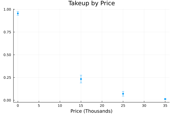
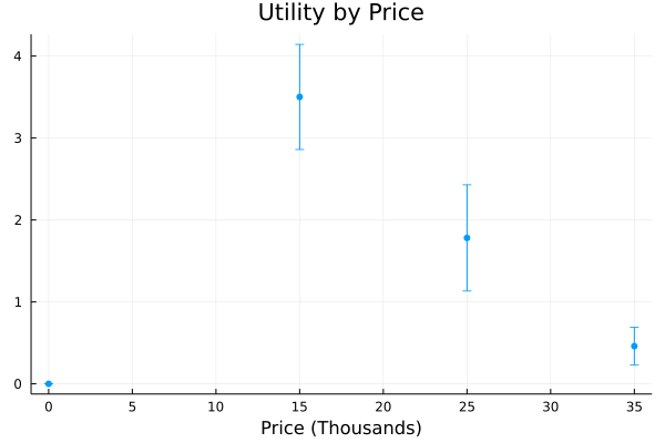
Figure 1: Takeup and utility by price

Mean estimated takeup and utility at each price included in the experiment of [17]. $95\%$ confidence intervals shown in bars.

For each $d$ in the experimental data, I plot the mean takeup and utility in Figure 1. Mean takeup $m_{0,P}(d)=\mathbb{E}_{P}[Y(d)]$ is identified from the experimental data for $d\in\mathcal{D}_{0}$, and estimated mean takeup $\hat{m}_{0}(d)$ is simply the sample mean at each price. Expected utility for experimental subsidy values is given by $v_{m_{P}}(d)=(\alpha-(35-d))m_{P}(d)$ and is estimated for $d\in\mathcal{D}_{0}$ by plugging in $\hat{m}_{0}(d)$. The price $d=0$ represents a fully subsidized connection, which is clearly undesireable from the decision maker’s perspective because the decision maker will recieve $0$ utility, which is the minimum possible, whether or not the household connects. Amongst the treatment values that appear in the data, $d=15$ achieves the highest utility on average. While not shown here, this is largely true of estimated mean utility conditional on $X$ as well. Indeed, setting $\mathcal{D}=\mathcal{D}_{0}$ and solving the empirical welfare maximization problem as in [15] with a linear eligibility score as the policy class assigns all individuals to a price of $15$.

A key question from the decision maker’s perspective is whether prices not in the support of $D$ in the data could yield higher utility, and how data from the experiment can provide information on the magnitude of such gains. To answer this, I impose shape restrictons which imply bounds on takeup at new prices. The shape restrictions I study here are that demand is downward sloping and the price subsidy exhibits diminishing returns. Takeup is also bounded between zero and one. Downward sloping demand is expected to be satisfied in all but a few exceptional markets, and represents one of the weaker assumptions a researcher may impose. Diminishing sensitivity to treatment may be more context specific, and can be motivated by a simple binary choice model where the density of valuations is decreasing on the support of treatments. Another setting where such a restriction may be applied is the analysis of production functions ([19]). The shape restrictions I impose, which can be expressed as linear inequalities involving the $J$-dimensional vector $m$ as shown in Appendix B, define the constraint $Sm\leq r$ in the linear program (5).

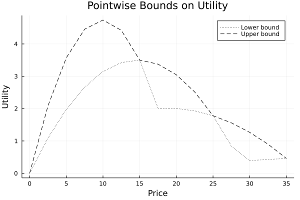
Figure 2: Bounds on takeup and utility at each price

The maximal and minimal possible expected takeup at each price, and the corresponding bounds on expected utility generated by these bounds on takeup.

To explore the potential effects of new treatments informally in the simple case of no covariates, in Figure 2 I plot pointwise upper and lower bounds on takeup at each possible price. These are obtained by calculating $\min_{m\in\hat{\mathcal{M}}}m(d)$ and $\max_{m\in\hat{\mathcal{M}}}m(d)$ for each $d$. Note that the lower bound is not convex. This is an illustration of the non-rectangularity induced by the shape restrictions– there is no $m\in\hat{\mathcal{M}}$ that simultaneously minimizes takeup for all prices $d$. More generally, not every curve that lies within the pointwise bounds of Figure 2 satisfies the shape restrictions. This can be expressed formally as

$$\hat{\mathcal{M}}\subset\bigg{\{}\tilde{m}\in\mathbbm{R}^{J}\mathrel{\mathop{\mathchar 58\relax}}\min_{m\in\hat{\mathcal{M}}}m\leq\tilde{m}_{j}\leq\max_{m\in\hat{\mathcal{M}}}m,\forall j\bigg{\}}$$

with strict containment. This difference is key for the informativeness of the linear program (5) because regret is defined by comparing the outcomes under the chosen policy to those of the first-best policy under the same demand curve $m$. If the chosen policy achieves low utility for one demand curve and the first-best policy achieves high utility only for a different demand curve, this does not contribute to high regret.

Along with the bounds on takeup in Figure 2, I also plot the bounds on expected utility $v_{m}$ generated by the bounds on takeup. These curves illustrate a range of possible outcomes that may result from implementing new treatments. The upper bounds on utility illustrate the potential for much better outcomes as a result of implementing new treatments, especially in the range of $7.5$ to $12.5$. The lower bounds imply the possibility of worse outcomes as well. A maximin welfare approach to this problem would not assign a price in $\mathcal{D}\setminus\mathcal{D}_{0}$ to anyone for whom that price was not guaranteed to outperform the prices in $\mathcal{D}$. This ends up assigning a price of $15$ to the entire sample, which seems excessively conservative in this example. On the other hand, the minimax regret approach considers losses relative to the ex-post optimal decision in each state of the world represented by $m\in\hat{\mathcal{M}}$.

Given the bounds in Figure 2, one could imagine naively constructing $\hat{\Gamma}_{jk}$ by comparing the worst possible $v_{m}(d_{j})$ to the best possible $v_{m}(d_{k})$. For example, taking $d_{k}=7.5$ and $d_{j}=10$ would result in an estimate of about $4.5-3.2=1.3$. However, recall that these bounds on $v_{m}$ were constructed from the bounds on $m$. Observing the bounds on $m$, it can be seen that the demand curve $m$ which achieves maximal takeup at $d=7.5$ and minimal takeup at $d=10$ is not convex, and thus the regret estimate obtained by comparing the pointwise bounds is unecessarily pessimistic. Likewise, taking $d_{k}=12.5$ and $d_{j}=10$ and comparing the pointwise bounds would yield an estimate of about $4.4-3.2=1.2$, but a demand curve which achieves these bounds is not decreasing. Formally, $\max_{m}[v_{m}(d_{k})-v_{m}(d_{j})]\leq\max_{m}v_{m}(d_{k})-\min_{m}v_{m}(d_{j})$. Thus, it is necessary to construct the regret estimates by finding a demand curve $m$ which maximizes regret while satisfying the shape restrictions. This illustrates that the linear program (5) defining $\hat{\Gamma}_{jk}$, while requiring more computations than pointwise bounds for each $d_{j}\in\mathcal{D}$, carries additional useful information.

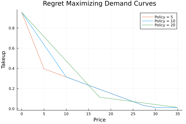
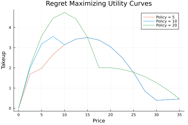
Figure 3: Regret-maximizing demand curves for alternative policies

The demand curves that maximize regret for each of three policies– assigning $d=5$ to everyone, assigning $d=10$ to everyone, and assigning $d=20$ to everyone. Also plotted are the utility curves generated by these regret-maximizing demand curves. Given a policy, the regret-maximizing demand curve is chosen to achieve low utility at the chosen price but high utility elsewhere.

To understand how maximal regret is computed for each policy, I plot regret-maximizing demand curves for each of three different policies in Figure 3. In this case, a policy is a single value of $d$ that will be assigned to the entire population. The regret-maximizing demand curve is the vector $m$ which solves (3) with no covariates. To compute it, I solve (5) for each $k$ and find the $m$ corresponding to the optimal $k$. Supposing the decision maker assigns a price of $d=5$ to the entire population, the regret-maximizing demand curve is chosen to yield low expected utility when $d=5$ but high utility for some other price, thus incurring high regret in the sense that the chosen policy of $d=5$ was ex-post a poor policy compared to, say, a price of $d=15$. The same process is enacted for the policies which assign $d=10$ to the entire population and $d=20$ to the entire population. Under the policy $d=20$, regret is very high because the difference between expected utility at $d=20$ and the optimal expected utility under the regret-maximizing demand curve is very large. Comparatively, the maximum regret incurred under the policy $d=10$ is small. Importantly, the regret-maximizing demand curves which generate these worst-case utility curves obey the shape restrictions, as can be seen in the left hand pane of Figure 3.

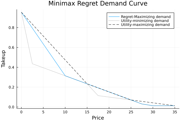
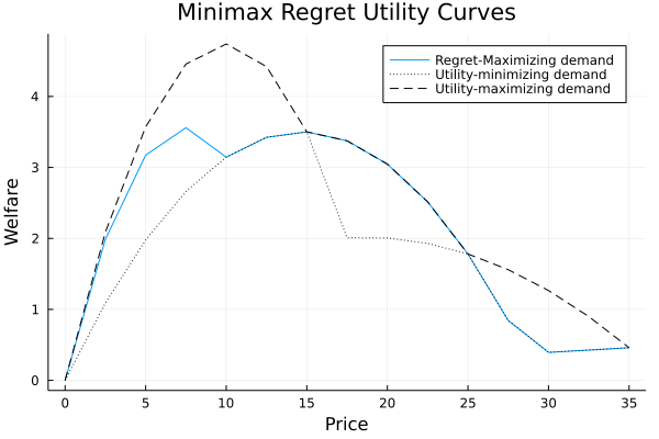
Figure 4: Regret-maximizing demand curves for $d=10$

The demand curve that achieves maximum regret under the minimax regret-optimal price of $d=10$ and the resulting welfare curve. The curves lie between the pointwise bounds examined in Figure 2.

Finally, I compute the optimal policy ignoring covariates. Across all policies, it turns out that the price $d=10$ has the smallest maximum regret. This means that across all demand curves $m\in\hat{\mathcal{M}}$, $v_{m}(10)$ is uniformly as close as possible to $\max_{d}v_{m}(d)$. To visualize this, in Figure 4 I overlay the regret-maximizing demand curve for the policy $d=10$ on top of the bounds on takeup and welfare plotted in Figure 2. The $m$ which maximizes regret is one which is maximized at $d=7.5$ but performs somewhat worse when $d=10$. This difference between the best possible outcome and the outcome realized under the chosen policy is the regret that nature seeks to maximize through the choice of $m$ and the decision maker seeks to minimize through the choice of $\pi$. Observe that maximum regret, given by $\max_{m}[v_{m}(7.5)-v_{m}(10)]$, is much smaller than a naive comparison of the bounds. Hence, an adversarially chosen demand curve in $\hat{\mathcal{M}}$ can make a price of $d=10$ perform only mildly suboptimally.

5.b Optimal Policy with Covariates

Having illustrated the method for estimating $\hat{m}_{0}$, constructing $\hat{\mathcal{M}}$, and constructing $\hat{\pi}$ in the simple case of no covariates, I now solve for the optimal policy when the decision maker can target subsidies based on household size and income. I construct the estimate $\hat{m}_{0}(d,x)$ using a logistic regression of takeup on a second order polynomial of household size and income, for each $d\in\mathcal{D}_{0}$. As before, I use the shape restrictions that demand is decreasing and convex in $d$, holding $x$ fixed. For less than $5\%$ of observations, the estimates $\hat{m}_{0}(d,X_{i})$ violate these shape restrictions. For these observations, I replace the estimates with $\arg\min_{m}\lVert m(d)-\hat{m}_{0}(d,X_{i})\rVert$, where the minimum is taken over all $m(d)\in\mathbbm{R}^{|\mathcal{D}_{0}|}$ that are decreasing and convex in $d$ and bounded between $0$ and $1$. This ensures that $\hat{\mathcal{M}}$ is nonempty. These estimates are used to obtain $\hat{\Gamma}_{j}(X_{i})$ for each $i$ and $j$.

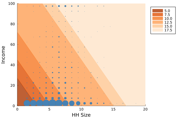
Figure 5: Optimal prices by covariates

The estimated optimal treatment allocation as a function of household size and earnings. The size of the dots is proportional to the number of people at each value of covariates. The shaded regions indicates which covariate values are assigned to each treatment.

Table 1: Optimal policy

$d$	5	7.5	10	12.5	15	17.5
% Treated	16%	20%	34%	24%	2.5%	2.7%
Cutoff	0.27	0.45	0.72	1.35	1.53	2.16
($\beta=[0.01,0.089]$)

Percent of population assigned to each treatment and eligibility score cutoff for each treatment for which a nonzero share of the population was assigned. Households were assigned to treatment $j$ if their score was below cutoff $j$ and above cutoff $j-1$.

Finally, to estimate the optimal policy, I consider a policy class of linear eligibility score rules where each treatment shares the same eligibility score, but different cutoffs. The decision maker chooses a vector of covariate weights $\beta$ and a vector of increasing cutoffs $c$. A household with covariates $X_{i}$ recieves treatment $d_{j}$ if $X_{i}^{\prime}\beta>c_{j-1}$ and $X_{i}^{\prime}\beta\leq c_{j}$, where $c_{0}=-\infty$ and $c_{J}=\infty$. I impose that the eligibility score increases with income, implying that poorer households recieve lower prices. Formally,

$$\Pi=\bigg{\{}\pi\mathrel{\mathop{\mathchar 58\relax}}\pi(x)=\sum_{j=1}^{J-1}(d_{j+1}-d_{j})\mathbbm{1}[X_{i}^{\prime}\beta>c_{j}],\;c_{j-1}\leq c_{j},\;\beta_{1}>0\bigg{\}}$$ (10)

Appendix B discusses how this class can be formulated with linear and integer constraints, resulting in a mixed integer-linear program formulation for the empirical minimax regret problem (4). The optimal allocation is illustrated in Figure 5, and exact estimates of the optimal policy along with the fraction of the population assigned to each treatment are presented in Table 1. The optimal allocation assigns poor, small households the lowest prices as they have the lowest willingness to pay. Almost the entire population is assigned a price not observed in the experimental data, with only $2.5\%$ of the population being assigned to the price $d=15$ which was optimal among the prices that were used in the experiment. Thus, a decision maker restricted to the support of the experimental data will achieve higher regret in this setting.

6 Conclusion

Experiments may not pilot all possible treatments a decision maker may consider. The existing literature on policy learning and treatment choice does not offer much guidance for how to use data on some treatment values to design policies involving new treatment values. I use data on previously observed treatments, partial identification, and the minimax regret criterion to extend empirical welfare maximization methods to settings where new treatments may be considered. Since the effects of new treatments are partially identified, a single policy is chosen to uniformly minimize regret across the identified set. The empirical minimax regret estimator is computationally tractable and posesses favorable regret convergence properties. In the setting of targeting subsidies to connect to the electrical grid, the estimator takes information on a small set of treatments and provides informative bounds on the effects of a much richer set new treatments, resulting in policies that implement new treatments which are uniformly close to optimal in every state of the world.

Appendix A Proofs

A.a Intermediary Results

I first introduce some notation and state existing results that I will use. Given a class of functions $\mathcal{F}$, the Rademacher complexity of $\mathcal{F}$ is defined as

$$\mathcal{R}_{N}(\mathcal{F})\mathrel{\mathop{\mathchar 58\relax}}=\mathbb{E}\bigg{[}\sup_{f\in\mathcal{F}}\bigg{|}\frac{1}{N}\sum_{i}\epsilon_{i}f(X_{i})\bigg{|}\bigg{]}$$

where $\epsilon_{i}$ are i.i.d. Rademacher random variables.

We say $\mathcal{T}$ is a $\delta$-cover of a metric space $(\mathcal{F},h)$ if for every $f\in\mathcal{F}$, there is some $f_{i}\in\mathcal{T}$ such that $h(f_{i},f)\leq\delta$. The cardinality of the smallest $\delta$-cover of $\mathcal{F}$ is called the $\delta$-covering number of $\mathcal{F}$ and is denoted $N(\delta,\mathcal{F},h)$.

I make use of the following existing results:

Lemma A.1.

([15] Lemma A.1) Let $\mathcal{G}$ be a VC-class of subsets of $\mathcal{X}$ with VC dimension $\mathbf{v}<\infty$. Let $g$ and $h$ be two given functions from $\mathcal{Y}\times\mathcal{D}\times\mathcal{X}$ to $\mathbbm{R}$. Then

$$\mathcal{F}=\{f\mathrel{\mathop{\mathchar 58\relax}}f(y,d,x)=g(y,d,x)\mathbbm{1}\{x\in G\}+h(y,d,x)\mathbbm{1}\{x\not\in G\},G\in\mathcal{G}\}$$

is a VC-subgraph class of functions with VC dimension less than or equal to $\mathbf{v}$.

Lemma A.2.

(Symmetrization) ([39] Lemma 2.3.1) For a class of measurable functions $\mathcal{F}$ and i.i.d random variables $X_{1},\dots,X_{N}$,

$$\mathbb{E}\bigg{[}\sup_{f\in\mathcal{F}}\bigg{|}\frac{1}{N}\sum_{i=1}^{N}f(X_{i})-\mathbb{E}[f(X_{i})]\bigg{|}\bigg{]}\leq 2\mathcal{R}_{N}(\mathcal{F})$$

Lemma A.3.

(Dudley’s entropy integral inequality) ([39] Corollary 2.2.8) Let $(Z_{f})_{f\in\mathcal{F}}$ be a separable process with sub-Gaussian increments. Then for some constant $K$, we have for any $f_{0}$

$$\mathbb{E}[\sup_{f\in\mathcal{F}}|Z_{f}|]\leq\mathbb{E}[|Z_{f_{0}}|]+K\int_{0}^{\infty}\sqrt{\log N(t,\mathcal{F},h)}dt$$

for some constant $K$.

Lemma A.4.

([39] Theorem 2.6.7) Suppose $\mathcal{F}$ is a VC-subgraph class with VC dimension at most $\mathbf{v}<\infty$ and suppose $\mathcal{F}$ has a measurable envelope function $F$. For $q\geq 1$ let $P$ be a probability measure such that $\lVert F\rVert_{q,P}>0$. Then

$$N(\delta\lVert F\rVert_{L_{q}(P)},\mathcal{F},L_{q}(P))\leq K\mathbf{v}(16e)^{\mathbf{v}}(1/\delta)^{q(\mathbf{v}-1)}$$

for some constant $K$ and $0<\delta<1$.

I now state and prove a useful result which establishes the relationship between the complexity of the policy class $\Pi$ and the complexity of the class of regret estimates. Define the following function classes:

$$\mathcal{F}\mathrel{\mathop{\mathchar 58\relax}}=\{f\mathrel{\mathop{\mathchar 58\relax}}f(x)=\sum_{j=1}^{J}\pi_{j}(x)\Gamma_{j}(x),\pi\in\Pi\}$$

$$\Pi_{j}\mathrel{\mathop{\mathchar 58\relax}}=\{\pi_{j}\mathrel{\mathop{\mathchar 58\relax}}\pi_{j}(x)=\mathbbm{1}[\pi(x)=d_{j}],\pi\in\Pi\},\quad\forall j\in\{1,\dots,J\}$$

The assumption that $\mathcal{F}$ is separable will be maintained.

Lemma A.5.

Under Assumption $\ref{DGP}.2$,

$$N(\delta,\mathcal{F},L_{2}(P_{N})) \leq\prod_{j=1}^{J}N(\epsilon,\Pi_{j},L_{2}(P_{N}))$$

where $\epsilon=\delta/(B\sqrt{J})$ and $B$ is the bound on $v(d,x)$ implied by Assumption 4.1.2.

Proof.

Let $f\in\mathcal{F}$ be given. From the discussion in Section 2, $f$ can be written as

$$f(x) =\max_{k}\max_{m\in\mathcal{M}_{P}}\bigg{(}v_{m}(d_{k},x)-\sum_{j=1}^{J}\pi_{j}(x)v_{m}(d_{j},x)\bigg{)}$$ (11)

for some $\pi\in\Pi$. For each treatment $j$, let $\mathcal{T}_{j}$ be a $\epsilon$-cover of $\Pi_{j}$ and let $\tilde{\pi}_{j}$ be an element of $\mathcal{T}_{j}$ satisfying $\mathbb{E}_{N}[(\pi_{j}(X)-\tilde{\pi}_{j}(X))^{2}]^{1/2}\leq\epsilon$. Define the approximating function $\tilde{f}$ by

$$\tilde{f}(x)=\max_{k}\max_{m\in\mathcal{M}_{P}}v_{m}(d_{k},x)-\sum_{j=1}^{J}\tilde{\pi}_{j}(x)v_{m}(d_{j},x)$$ (12)

Finally, let $k^{*},m^{*}(x)$ be maximizers of (11) and let $\tilde{k},\tilde{m}(x)$ be maximizers of (12).

For each $x$ we have by the optimality of $k^{*}$ and $m^{*}$

$$f(x)-\tilde{f}(x) =v_{m^{*}}(d_{k^{*}},x)-v_{\tilde{m}}(d_{\tilde{k}},x)+\sum_{j=1}^{J}\bigg{[}\tilde{\pi}_{j}(x)v_{m^{*}}(d_{j},x)-\pi_{j}(x)v_{\tilde{m}}(d_{j},x)\bigg{]}$$

$$\geq v_{\tilde{m}}(d_{\tilde{k}},x)-v_{\tilde{m}}(d_{\tilde{k}},x)+\sum_{j=1}^{J}\bigg{[}\tilde{\pi}_{j}(x)v_{\tilde{m}}(d_{j},x)-\pi_{j}(x)v_{\tilde{m}}(d_{j},x)\bigg{]}$$

$$=\sum_{j=1}^{J}\bigg{[}(\tilde{\pi}_{j}(x)-\pi_{j}(x))v_{\tilde{m}}(d_{j},x)\bigg{]}$$

Likewise, optimality of $\tilde{m}$ and $\tilde{k}$ imply

$$f(x)-\tilde{f}(x) \leq\sum_{j=1}^{J}\bigg{[}(\tilde{\pi}_{j}(x)-\pi_{j}(x))v_{m^{*}}(d_{j},x)\bigg{]}$$

Together, we have

$$|f(x)-\tilde{f}(x)| \leq\max\bigg{\{}\bigg{|}\sum_{j=1}^{J}(\tilde{\pi}_{j}(x)-\pi_{j}(x))v_{\tilde{m}}(d_{j},x)\bigg{|},\bigg{|}\sum_{j=1}^{J}(\tilde{\pi}_{j}(x)-\pi_{j}(x))v_{m^{*}}(d_{j},x)\bigg{|}\bigg{\}}$$

$$\leq\max\bigg{\{}\lVert(\tilde{\pi}_{j}(x)-\pi_{j}(x))_{j=1}^{j}\rVert\lVert v_{\tilde{m}}(.,x)\rVert,\lVert(\tilde{\pi}_{j}(x)-\pi_{j}(x))_{j=1}^{j}\rVert\lVert v_{m^{*}}(.,x)\rVert\bigg{\}}$$

$$\leq B\bigg{(}\sum_{j}(\pi_{j}(x)-\tilde{\pi}_{j}(x))^{2}\bigg{)}^{1/2}$$

where the second line is by the Cauchy-Schwartz inequality. Squaring and integrating over $x$,

$$\mathbb{E}_{N,P}[(f(X)-\tilde{f}(X))^{2}] \leq B^{2}\mathbb{E}_{N,P}\bigg{[}\sum_{j}(\pi_{j}(X)-\tilde{\pi}_{j}(X))^{2}\bigg{]}$$

$$\leq B^{2}J\epsilon^{2}$$

$$\leq\delta^{2}$$

Taking the square root of both sides shows that $\lVert f-\tilde{f}\rVert_{L_{2}(P_{N})}\leq\delta$. Consider the set of all such functions constructed this way,

$$\mathcal{T}\mathrel{\mathop{\mathchar 58\relax}}=\bigg{\{}\tilde{f}\mathrel{\mathop{\mathchar 58\relax}}\tilde{f}(x)=\max_{k}\max_{m\in\mathcal{M}}v_{m}(d_{k},x)-\sum_{j=1}^{J}\tilde{\pi}_{j}(x)v_{m}(d_{j},x),\;\tilde{\pi}=(\tilde{\pi}_{1},\dots,\tilde{\pi}_{J}),\tilde{\pi}_{j}\in\mathcal{T}_{j}\bigg{\}}$$

we see that $|\mathcal{T}|=\prod_{j}|\mathcal{T}_{j}|$, and $\mathcal{T}$ is a $\delta$-cover of $\mathcal{F}$. ∎

We can now prove the main results of the paper.

A.b Proof of Lemma 4.5

Proof.

To simplify notation, for now we consider $P$ fixed and supress dependence on $P$. By the definition of $\mathcal{F}$, we have

$$\mathbb{E}\bigg{[}\sup_{\pi\in\Pi}\bigg{|}\overline{R}(\pi)-\tilde{R}_{N}(\pi)\bigg{|}\bigg{]}=\mathbb{E}\bigg{[}\sup_{f\in\mathcal{F}}\bigg{|}\frac{1}{N}\sum_{i=1}^{N}f(X_{i})-\mathbb{E}[f(X_{i})]\bigg{|}\bigg{]}$$

Hence, we can apply Lemma A.2 to obtain

$$\mathbb{E}\bigg{[}\sup_{\pi\in\Pi}\bigg{|}\overline{R}(\pi)-\tilde{R}_{N}(\pi)\bigg{|}\bigg{]} \leq 2\mathcal{R}_{N}(\mathcal{F})$$

Now, define $Z_{f}=\frac{1}{\sqrt{N}}\sum_{i=1}^{N}\epsilon_{i}f(X_{i})$. The increments of $(Z_{f})_{f\in\mathcal{F}}$ are given by $\frac{1}{\sqrt{N}}\sum_{i=1}^{N}\epsilon_{i}(f(X_{i})-g(X_{i}))$. Conditional on $(X_{i})_{i=1}^{N}$, we can apply Hoeffding’s inequality (e.g. [39] Lemma 2.2.7) to establish that this is sub-Gaussian with parameter $\left(\frac{1}{N}\sum_{i=1}^{N}(f(X_{i})-g(X_{i}))^{2}\right)^{1/2}=\lVert f-g\rVert_{L_{2}(P_{N})}$. We can then apply Lemma A.3 conditional on $(X_{i})_{i=1}^{N}$ to obtain

$$\frac{1}{\sqrt{N}}\mathbb{E}_{\epsilon}[\sup_{f\in\mathcal{F}}|Z_{f}|] \leq\frac{1}{\sqrt{N}}\mathbb{E}_{\epsilon}[|Z_{f_{0}}|]+\frac{K}{\sqrt{N}}\int_{0}^{\infty}\sqrt{\log N(t,\mathcal{F},L_{2}(P_{N}))}dt$$

for some $f_{0}\in\mathcal{F}$. Moreover, since $f_{0}$ is bounded by $2B$, $|Z_{f_{0}}|\leq|\sum_{i=1}^{N}\epsilon_{i}\frac{2B}{\sqrt{N}}|$. Again by Hoeffding’s inequality, this implies that $Z_{f_{0}}$ is sub-Gaussian with parameter $K^{\prime}\left(\frac{1}{N}\sum_{i=1}^{N}(2B)^{2}\right)^{1/2}=K^{\prime}2B$ which does not depend on $N$. Basic properties of sub-Gaussian random variables (e.g. [40] Proposition 2.5.2) imply that $\mathbb{E}_{\epsilon}[|Z_{f_{0}}|]\leq K^{\prime\prime}$ for some constant $K^{\prime\prime}$. Thus,

$$\frac{1}{\sqrt{N}}\mathbb{E}_{\epsilon}[\sup_{f\in\mathcal{F}}|Z_{f}|] \leq\frac{1}{\sqrt{N}}\left(K^{\prime\prime}+K\int_{0}^{\infty}\sqrt{\log N(t,\mathcal{F},L_{2}(P_{N}))}dt\right)$$

$$=\frac{1}{\sqrt{N}}\left(K^{\prime\prime}+K\int_{0}^{4B}\sqrt{\log N(t,\mathcal{F},L_{2}(P_{N}))}dt\right)$$

where we have used the fact that since the diameter of $\mathcal{F}$ is $2B$, the integrand is $0$ for $t>4B$. By Lemma A.1, each class $\Pi_{j}$ is a VC-subgraph class of functions with VC dimension at most $v$. Then applying Lemma A.5 and a change of variables yields

$$\frac{1}{\sqrt{N}}\mathbb{E}_{\epsilon}[\sup_{f\in\mathcal{F}}|Z_{f}|] \leq\frac{1}{\sqrt{N}}\left(K^{\prime\prime}+K\int_{0}^{4/\sqrt{J}}\sqrt{\sum_{j}\log N(t,\Pi_{j},L_{2}(P_{N}))}B\sqrt{J}dt\right)$$

Apply Lemma A.4 to each VC-subgraph class of functions $\Pi_{j}$, which have envelope $1$, and allow $K$ to subsume other constants to obtain

$$\frac{1}{\sqrt{N}}\mathbb{E}_{\epsilon}[\sup_{f\in\mathcal{F}}|Z_{f}|] \leq\frac{1}{\sqrt{N}}\left(K^{\prime\prime}+K\int_{0}^{4/\sqrt{J}}\sqrt{\log K\mathbf{v}(16e)^{\mathbf{v}}(1/t)^{2(\mathbf{v}-1)}}dt\right)$$ (13)

$$\leq\frac{1}{\sqrt{N}}\left(K^{\prime\prime}+K\sqrt{\mathbf{v}}\right)$$ (14)

$$\leq K\sqrt{\frac{v}{N}}$$ (15)

Finally, since $\mathcal{R}_{N}(\mathcal{F})=\mathbb{E}[\frac{1}{\sqrt{N}}\mathbb{E}_{\epsilon}[\sup_{f\in\mathcal{F}}|Z_{f}|]]$, we obtain

$$\mathbb{E}\bigg{[}\sup_{\pi\in\Pi}\bigg{|}\overline{R}(\pi)-\tilde{R}_{N}(\pi)\bigg{|}\bigg{]} \leq K\sqrt{\frac{\mathbf{v}}{N}}$$

Note that the constant $K$ does depend on $B$ and $J$. ∎

A.c Proof of Lemma 4.6

Proof.

To simplify notation, for now we consider $P$ fixed and supress dependence on $P$. For every $1\leq j,k\leq J$, let $\gamma_{jk}\mathrel{\mathop{\mathchar 58\relax}}\mathbbm{R}^{J_{0}}\mapsto 2^{\mathbbm{R}^{J}}$ be the identified set for covariate-level regret, viewed as a set-valued mapping from the first stage conditional mean response vector to subsets of $\mathbbm{R}^{J}$. That is, hold $x$ fixed and define $\gamma_{jk}(w)=\{b_{jk}(x)^{\prime}m-c_{jk}(x)\mathrel{\mathop{\mathchar 58\relax}}Fm=w,Sm\leq r\}$. For this proof, we view $\Gamma_{jk}$ as a function of the first stage conditional mean response $m_{0}$ to consider how $\Gamma_{jk}$ changes with perturbations to $m_{0}$. Thus, $\Gamma_{jk}(m_{0}(\cdot,X_{i}))=\max\{\gamma_{jk}(m_{0}(\cdot,X_{i}))\}$.

For any matrix $A$, let $A^{\dagger}\mathrel{\mathop{\mathchar 58\relax}}\text{null}(A)^{\perp}\mapsto\text{range}(A)$ denote the Moore-Penrose pseudoinverse operator, where $\text{null}(A)$ and $\text{range}(A)$ denote the nullspace and range of $A$, respectively. For any $w\in\mathbbm{R}^{J_{0}}$,

$$\{m\mathrel{\mathop{\mathchar 58\relax}}Fm=w\}=\{m\mathrel{\mathop{\mathchar 58\relax}}m=F^{\dagger}w+y,\;y\in\text{null}(F)\}$$

Let $\tilde{w}\in\mathbbm{R}^{J_{0}}$ be given. For any $J$, let $\mathcal{B}_{J}$ be the unit ball in $\mathbbm{R}^{J}$, $\mathcal{B}_{J}\mathrel{\mathop{\mathchar 58\relax}}=\{w\in\mathbbm{R}^{J}\mathrel{\mathop{\mathchar 58\relax}}\lVert w\rVert\leq 1\}$. Since $\tilde{w}\in w+\lVert w-\tilde{w}\rVert\mathcal{B}_{J_{0}}$,

$$\{m\mathrel{\mathop{\mathchar 58\relax}}m=F^{\dagger}\tilde{w}+y,\;y\in\text{null}(F)\} \subseteq\{m\mathrel{\mathop{\mathchar 58\relax}}m=F^{\dagger}z+y,\;y\in\text{null}(F),\;z\in w+\lVert w-\tilde{w}\rVert\mathcal{B}_{J_{0}}\}$$

$$\subseteq\{m\mathrel{\mathop{\mathchar 58\relax}}m=F^{\dagger}w+y,\;y\in\text{null}(F)\}+\lVert F^{\dagger}\rVert\lVert\tilde{w}-w\rVert\mathcal{B}_{J}\}$$

where $\lVert F^{\dagger}\rVert$ denotes the operator norm of $F^{\dagger}$. This implies

$$\{m\mathrel{\mathop{\mathchar 58\relax}}Fm=\tilde{w}\}\cap\{m\mathrel{\mathop{\mathchar 58\relax}}Sm\leq r\}\subseteq\left(\{m\mathrel{\mathop{\mathchar 58\relax}}m=F^{\dagger}w+y,y\in\text{null}(F)\}+\lVert F^{\dagger}\rVert\lVert\tilde{w}-w\rVert\mathcal{B}_{J}\right)\cap\{m\mathrel{\mathop{\mathchar 58\relax}}Sm\leq r\}$$

and since $\gamma_{jk}(\tilde{w})$ consists of scalars of the form $b_{jk}(x)^{\prime}m-c_{jk}(x)$ for $m$ in this set, we have

$$\gamma_{jk}(\tilde{w}) \subseteq\gamma_{jk}(w)+\lVert b_{jk}(x)\rVert\lVert F^{\dagger}\rVert\lVert\tilde{w}-w\rVert\mathcal{B}_{1}$$

and likewise

$$\gamma_{jk}(w)\subseteq\gamma_{jk}(\tilde{w})+\lVert b_{jk}(x)\rVert\lVert F^{\dagger}\rVert\lVert\tilde{w}-w\rVert\mathcal{B}_{1}$$

Therefore, the correspondence $\gamma_{jk}$ is Lipschitz with respect to the Hausdorff distance, with Lipschitz constant $\sup_{x}\lVert b_{jk}(x)\rVert\lVert F^{\dagger}\rVert\mathrel{\mathop{\mathchar 58\relax}}=\kappa<\infty$ (Rockafellar and Wets 2005). Importantly, this implies $|\Gamma_{jk}(\hat{m}_{0}(\cdot,X_{i})-\Gamma_{jk}(m_{0}(\cdot,X_{i}))|\leq\kappa\lVert\hat{m}_{0}(\cdot,X_{i})-m_{0}(\cdot,X_{i})\rVert$. While not essential to our analysis, we note that in our case $\lVert F^{\dagger}\rVert=1$.

We can now prove the main claim of the lemma.

$$\mathbb{E}\bigg{[}\sup_{\pi\in\Pi}\bigg{|}\tilde{R}_{N}(\pi)-\overline{R}_{N}(\pi)\bigg{|}\bigg{]}$$

$$=\mathbb{E}\bigg{[}\sup_{\pi\in\Pi}\bigg{|}\frac{1}{N}\sum_{i=1}^{N}\sum_{j=1}^{J}\pi_{ij}(\max_{k}\Gamma_{jk}(\hat{m}_{0}(\cdot,X_{i}))-\max_{k}\Gamma_{jk}(m_{0}(\cdot,X_{i})))\bigg{|}\bigg{]}$$

$$\leq\mathbb{E}\bigg{[}\frac{1}{N}\sum_{i=1}^{N}\max_{j,k}\bigg{|}\Gamma_{jk}(\hat{m}_{0}(\cdot,X_{i}))-\Gamma_{jk}(m_{0}(\cdot,X_{i}))\bigg{|}\bigg{]}$$

$$\leq\mathbb{E}\bigg{[}\frac{1}{N}\sum_{i=1}^{N}\kappa\lVert\hat{m}_{0}(\cdot,X_{i})-m_{0}(\cdot,X_{i})\rVert\bigg{]}$$

Finally, we bound this uniformly in $P$ by Assumption 4.2. We conclude that

$$\sup_{P\in\mathcal{P}_{C}}\mathbb{E}_{P}\bigg{[}\sup_{\pi\in\Pi}\bigg{|}\tilde{R}_{N,P}(\pi)-\overline{R}_{N}(\pi)\bigg{|}\bigg{]} \leq\mathcal{O}(\rho_{N}^{-1})$$

∎

Appendix B Computational Details

B.a Shape Constraints

Mean takeup as a function of price, holding covariates fixed, is bounded between $0$ and $1$. It is assumed to be downward sloping and the subsidy is assumed to exhibit decreasing returns to scale, so that takeup is convex. These constraints can be expressed as $S\tilde{m}(.,X)\leq r$ where

$$S_{1}=\begin{bmatrix}\frac{-1}{d_{2}-d_{1}}&\frac{1}{d_{2}-d_{1}}&0&\dots\\ 0&\frac{-1}{d_{3}-d_{2}}&\frac{1}{d_{3}-d_{2}}&0&\dots\\ \vdots\\ &&&&\dots&0&\frac{-1}{d_{J}-d_{J-1}}&\frac{1}{d_{J}-d_{J-1}}\end{bmatrix}$$

$$S_{2}=\begin{bmatrix}\frac{-1}{d_{2}-d_{1}}&\frac{1}{d_{2}-d_{1}}+\frac{1}{d_{3}-d_{2}}&\frac{-1}{d_{3}-d_{2}}&0&\dots\\ 0&\frac{-1}{d_{3}-d_{2}}&\frac{1}{d_{3}-d_{2}}+\frac{1}{d_{4}-d_{3}}&\frac{-1}{d_{4}-d_{3}}&0&\dots\\ \vdots\\ &&&&\dots&0&\frac{-1}{d_{J-1}-d_{J-2}}&\frac{1}{d_{J-1}-d_{J-2}}+\frac{1}{d_{J}-d_{J-1}}&\frac{-1}{d_{J}-d_{J-1}}\end{bmatrix}$$

$$S=\begin{bmatrix}-I\\ I\\ S_{1}\\ S_{2}\end{bmatrix}\quad\quad r=\begin{bmatrix}0_{J}\\ -1_{J}\\ 0_{J-1}\\ 0_{J-2}\end{bmatrix}$$

B.b Dual Representaion of Maximum Regret

For each individual $i$, the maximum regret is obtained by

$$\hat{\Gamma}_{j}(X_{i}) =\max_{k,m}b_{jk}(X_{i})^{\prime}m-c_{jk}(X_{i})\quad s.t.\quad Sm\leq r,\quad Fm=\hat{m}(.,X_{i})$$

For now, supress the dependence on $X_{i}$ and $j$. Let $\lambda$ be the vector of Lagrange dual variables associated with the inequality constraint, and let $\eta$ be the vector of Lagrange dual variables associated with the equality constraint. We can rewrite the linear program as

$$\min_{\mu}\mu\quad s.t.\quad\mu+c_{k}\geq\max_{m}\{b_{k}^{\prime}m\quad s.t.\quad Sm\leq r,Fm=\hat{m}_{0}\}\quad\forall k$$

$$\min_{\mu}\mu\quad s.t.\quad\mu+c_{k}\geq\min_{\lambda,\eta}\{\lambda^{\prime}r+\eta^{\prime}\hat{m}_{0}\quad s.t.\quad\lambda^{\prime}S+\eta^{\prime}F\geq b_{k},\quad\lambda\geq 0\}\forall k$$

$$\min_{\mu,\lambda,\eta}\mu\quad s.t.\quad\mu+c_{k}\geq\lambda^{\prime}r+\eta^{\prime}\hat{m}_{0},\quad\lambda^{\prime}S+\eta^{\prime}F\geq b_{k},\quad\lambda\geq 0\quad\forall k$$

Thus, computing each $\hat{\Gamma}_{j}(X_{i})$ is a single linear program. Since the programs are independent across $i$, they can be solved simultaneously by summing the objective across individuals.

This strategy can be extended to compute all $\hat{\Gamma}_{j}(X_{i})$ across $i$ and $j$ simultaneously, and even in the same mixed integer-linear program that chooses the optimal policy $\pi$. However, this did not decrease computation time in the application of Section 5.

B.c MILP Formulation of MMR Problem

Consider the set of policies given by (10) and the problem (4). To express this as a mixed integer-linear program, introduce the binary variables $g_{ij}$ for $i=1,\dots,N$ and $j=1,\dots,J-1$ to indicate whether $X_{i}^{\prime}\beta$ is above cutoff $j$. For notational convenience, set $g_{i0}=1$ and $g_{iJ}=0$

$$\min_{g,\beta,c} \sum_{i=1}^{N}\sum_{j=1}^{J}(g_{ij}-g_{i,j-1})\hat{\Gamma}_{j}(X_{i})$$

$$s.t.\quad c_{1}\leq c_{2}\leq\dots\leq c_{J-1}$$

$$g_{ij}\geq X_{i}^{\prime}\beta-c_{j}+\epsilon,\quad i=1,\dots,N,\quad j=1,\dots,J-1$$

$$g_{ij}\leq 1+X_{i}^{\prime}\beta-c_{j},\quad i=1,\dots,N,\quad j=1,\dots,J-1$$

$$\beta_{1}\geq 0$$

where $\epsilon$ is a sufficiently small numerical error term. To help with numerical stability, $\beta_{1}$ can be fixed to be a constant, resulting in a rescaling of $c_{j}$ and $\beta_{2}$.

Appendix C Robustness

In these section I present the optimal policy under different specifications of $\mathcal{D}$ and $\alpha$. I examine a “Coarse” treatment set $\mathcal{D}=\{0,5,10,\dots,35\}$, the “Baseline” treatment set $\mathcal{D}=\{0,2.5,5,\dots,35\}$, and a “Fine” treatment set $\mathcal{D}=\{0,1,2,\dots,35\}$. For each treatment set I consider $\alpha\in\{25,35,45\}$, except for $\alpha=35$ under the Baseline treatment set, which is identical to the main text. The results are plotted in Figures 6-13.

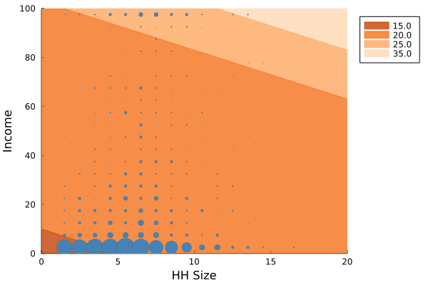
Figure 6: Coarse $\mathcal{D}$, $\alpha=25$

The estimated optimal treatment allocation as a function of household size and earnings. The size of the dots is proportional to the number of people at each value of covariates. The shaded regions indicates which covariate values are assigned to each treatment.

Figure 7: Baseline $\mathcal{D}$, $\alpha=25$

The estimated optimal treatment allocation as a function of household size and earnings. The size of the dots is proportional to the number of people at each value of covariates. The shaded regions indicates which covariate values are assigned to each treatment.

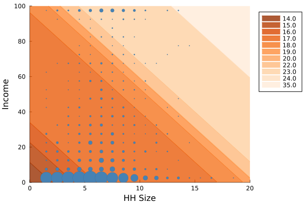
Figure 8: Fine $\mathcal{D}$, $\alpha=25$

The estimated optimal treatment allocation as a function of household size and earnings. The size of the dots is proportional to the number of people at each value of covariates. The shaded regions indicates which covariate values are assigned to each treatment.

Figure 9: Coarse $\mathcal{D}$, $\alpha=35$

The estimated optimal treatment allocation as a function of household size and earnings. The size of the dots is proportional to the number of people at each value of covariates. The shaded regions indicates which covariate values are assigned to each treatment.

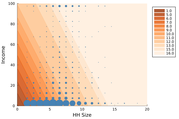
Figure 10: Fine $\mathcal{D}$, $\alpha=35$

The estimated optimal treatment allocation as a function of household size and earnings. The size of the dots is proportional to the number of people at each value of covariates. The shaded regions indicates which covariate values are assigned to each treatment.

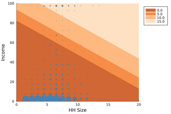
Figure 11: Coarse $\mathcal{D}$, $\alpha=45$

The estimated optimal treatment allocation as a function of household size and earnings. The size of the dots is proportional to the number of people at each value of covariates. The shaded regions indicates which covariate values are assigned to each treatment.

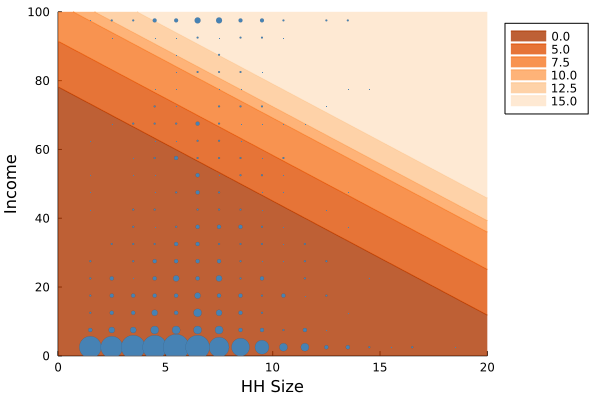
Figure 12: Baseline $\mathcal{D}$, $\alpha=45$

The estimated optimal treatment allocation as a function of household size and earnings. The size of the dots is proportional to the number of people at each value of covariates. The shaded regions indicates which covariate values are assigned to each treatment.

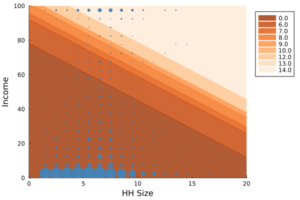
Figure 13: Fine $\mathcal{D}$, $\alpha=45$

The estimated optimal treatment allocation as a function of household size and earnings. The size of the dots is proportional to the number of people at each value of covariates. The shaded regions indicates which covariate values are assigned to each treatment.

References

- [1] Susan Athey and Stefan Wager “Policy learning with observational data” In Econometrica 89.1 Wiley Online Library, 2021, pp. 133–161
- [2] Eli Ben-Michael, D James Greiner, Kosuke Imai and Zhichao Jiang “Safe policy learning through extrapolation: Application to pre-trial risk assessment” In arXiv preprint arXiv:2109.11679, 2021
- [3] Debopam Bhattacharya and Pascaline Dupas “Inferring welfare maximizing treatment assignment under budget constraints” In Journal of Econometrics 167.1 Elsevier, 2012, pp. 168–196
- [4] Denis Chetverikov, Andres Santos and Azeem M Shaikh “The econometrics of shape restrictions” In Annual Review of Economics 10.1 Annual Reviews, 2018, pp. 31–63
- [5] Timothy Christensen, Hyungsik Roger Moon and Frank Schorfheide “Optimal Discrete Decisions when Payoffs are Partially Identified” In arXiv preprint arXiv:2204.11748, 2022
- [6] Riccardo D’Adamo “Policy Learning Under Ambiguity” In arXiv preprint arXiv:2111.10904, 2021
- [7] Zheng Fang, Andres Santos, Azeem Shaikh and Alexander Torgovitsky “Inference for large-scale linear systems with known coefficients” In University of Chicago, Becker Friedman Institute for Economics Working Paper, 2020
- [8] Joachim Freyberger and Joel L Horowitz “Identification and shape restrictions in nonparametric instrumental variables estimation” In Journal of Econometrics 189.1 Elsevier, 2015, pp. 41–53
- [9] James J Heckman and Edward J Vytlacil “Econometric evaluation of social programs, part I: Causal models, structural models and econometric policy evaluation” In Handbook of econometrics 6 Elsevier, 2007, pp. 4779–4874
- [10] Keisuke Hirano and Jack R Porter “Asymptotics for statistical treatment rules” In Econometrica 77.5 Wiley Online Library, 2009, pp. 1683–1701
- [11] Keisuke Hirano and Jack R Porter “Asymptotic analysis of statistical decision rules in econometrics” In Handbook of Econometrics 7 Elsevier, 2020, pp. 283–354
- [12] Alan J Hoffman “On approximate solutions of systems of linear inequalities” In Selected Papers Of Alan J Hoffman: With Commentary World Scientific, 2003, pp. 174–176
- [13] Nathan Kallus and Angela Zhou “Policy evaluation and optimization with continuous treatments” In International conference on artificial intelligence and statistics, 2018, pp. 1243–1251 PMLR
- [14] Nathan Kallus and Angela Zhou “Minimax-optimal policy learning under unobserved confounding” In Management Science 67.5 INFORMS, 2021, pp. 2870–2890
- [15] Toru Kitagawa and Aleksey Tetenov “Who should be treated? empirical welfare maximization methods for treatment choice” In Econometrica 86.2 Wiley Online Library, 2018, pp. 591–616
- [16] Kenneth Lee, Edward Miguel and Catherine Wolfram “Does household electrification supercharge economic development?” In Journal of Economic Perspectives 34.1, 2020, pp. 122–44
- [17] Kenneth Lee, Edward Miguel and Catherine Wolfram “Experimental evidence on the economics of rural electrification” In Journal of Political Economy 128.4 The University of Chicago Press Chicago, IL, 2020, pp. 1523–1565
- [18] Yan Liu “Policy Learning under Endogeneity Using Instrumental Variables” In arXiv preprint arXiv:2206.09883, 2022
- [19] Charles F Manski “Monotone treatment response” In Econometrica: Journal of the Econometric Society JSTOR, 1997, pp. 1311–1334
- [20] Charles F Manski “Statistical treatment rules for heterogeneous populations” In Econometrica 72.4 Wiley Online Library, 2004, pp. 1221–1246
- [21] Charles F Manski “Search profiling with partial knowledge of deterrence” In The Economic Journal 116.515 Oxford University Press Oxford, UK, 2006, pp. F385–F401
- [22] Charles F Manski “Minimax-regret treatment choice with missing outcome data” In Journal of Econometrics 139.1 Elsevier, 2007, pp. 105–115
- [23] Charles F Manski “Identification for prediction and decision” Harvard University Press, 2009
- [24] Charles F Manski “Vaccination with partial knowledge of external effectiveness” In Proceedings of the National Academy of Sciences 107.9 National Acad Sciences, 2010, pp. 3953–3960
- [25] Charles F Manski “Choosing treatment policies under ambiguity” In Annu. Rev. Econ. 3.1 Annual Reviews, 2011, pp. 25–49
- [26] Charles F Manski “Econometrics for decision making: Building foundations sketched by haavelmo and wald” In Econometrica 89.6 Wiley Online Library, 2021, pp. 2827–2853
- [27] Charles F Manski “Using Limited Trial Evidence to Credibly Choose Treatment Dosage when Efficacy and Adverse Effects Weakly Increase with Dose”, 2023
- [28] Eric Mbakop and Max Tabord-Meehan “Model selection for treatment choice: Penalized welfare maximization” In Econometrica 89.2 Wiley Online Library, 2021, pp. 825–848
- [29] Magne Mogstad, Andres Santos and Alexander Torgovitsky “Using instrumental variables for inference about policy relevant treatment parameters” In Econometrica 86.5 Wiley Online Library, 2018, pp. 1589–1619
- [30] Jörg Peters and Maximiliane Sievert “Impacts of rural electrification revisited–the African context” In Journal of Development Effectiveness 8.3 Taylor & Francis, 2016, pp. 327–345
- [31] Hongming Pu and Bo Zhang “Estimating optimal treatment rules with an instrumental variable: A partial identification learning approach” In Journal of the Royal Statistical Society: Series B (Statistical Methodology) 83.2 Wiley Online Library, 2021, pp. 318–345
- [32] Min Qian and Susan A Murphy “Performance guarantees for individualized treatment rules” In Annals of statistics 39.2 NIH Public Access, 2011, pp. 1180
- [33] R Tyrrell Rockafellar and Roger J-B Wets “Variational analysis” Springer ScienceBusiness Media, 2009
- [34] Thomas M Russell “Policy transforms and learning optimal policies” In arXiv preprint arXiv:2012.11046, 2020
- [35] Yuya Sasaki and Takuya Ura “Welfare analysis via marginal treatment effects” In arXiv preprint arXiv:2012.07624, 2020
- [36] Leonard J Savage “The theory of statistical decision” In Journal of the American Statistical association 46.253 Taylor & Francis, 1951, pp. 55–67
- [37] Jörg Stoye “Minimax regret treatment choice with covariates or with limited validity of experiments” In Journal of Econometrics 166.1 Elsevier, 2012, pp. 138–156
- [38] Dominique Van de Walle, Martin Ravallion, Vibhuti Mendiratta and Gayatri Koolwal “Long-term gains from electrification in rural India” In The World Bank Economic Review 31.2 Oxford University Press, 2017, pp. 385–411
- [39] AW van der Vaart and JA Wellner “Empirical Processes and Weak Convergence” Springer, New York, 1996
- [40] Roman Vershynin “High-dimensional probability: An introduction with applications in data science” Cambridge university press, 2018
- [41] Abraham Wald “Statistical decision functions.” Wiley, 1950
- [42] Kohei Yata “Optimal Decision Rules Under Partial Identification” In arXiv preprint arXiv:2111.04926, 2021
- [43] Baqun Zhang et al. “Estimating optimal treatment regimes from a classification perspective” In Stat 1.1 Wiley Online Library, 2012, pp. 103–114
- [44] Yi Zhang, Eli Ben-Michael and Kosuke Imai “Safe Policy Learning under Regression Discontinuity Designs” In arXiv preprint arXiv:2208.13323, 2022
- [45] Yingqi Zhao, Donglin Zeng, A John Rush and Michael R Kosorok “Estimating individualized treatment rules using outcome weighted learning” In Journal of the American Statistical Association 107.499 Taylor & Francis, 2012, pp. 1106–1118
- [46] Zhengyuan Zhou, Susan Athey and Stefan Wager “Offline multi-action policy learning: Generalization and optimization” In arXiv preprint arXiv:1810.04778, 2018