s O1 O O O Ofigure m[#4]#3

‘Sawfish’ Photonic Crystal Cavity for Near-Unity Emitter-to-Fiber Interfacing in Quantum Network Applications

A. Debye-Waller factor estimation

The procedure outlined in the following yields the Debye-Waller factors used in the main article to determine the cavity-enhanced ratio of light emitted into the respective emitter’s zero-phonon line (ZPL).

A.1 Group-IV vacancy centers

The total decay rate from level $|3\rangle$ (LABEL:fig:SnVRateModel) for a negatively-charged group-IV vacancy center in diamond (G4V) [1] is

$$\gamma=\gamma_{32}+\gamma_{31}+\gamma_{\mathrm{PSB}}\,,$$ (1)

where $\gamma_{\mathrm{PSB}}=\sum_{k}\gamma_{31_{k}}$ is the relaxation rate into the phonon sideband (PSB). In general, it is

$$\gamma_{\mathrm{ZPL}}=\gamma_{32}+\gamma_{31}=DW_{\mathrm{G4V}}^{0}/\tau\,,$$ (2)

$$\gamma_{\mathrm{PSB}}=(1-DW_{\mathrm{G4V}}^{0})/\tau\,,$$ (3)

where $\tau=1/\gamma$ is the excited state lifetime. The Debye-Waller factor in absence of Purcell enhancement is defined as

$$DW_{\mathrm{G4V}}^{0}=\frac{\gamma_{\mathrm{ZPL}}}{\gamma}=\frac{\gamma_{31}+\gamma_{32}}{\gamma}\,.$$ (4)

Tab. 1 of the main article lists $DW_{\mathrm{G4V}}^{0}$ for different G4Vs. It is assumed that $Q>$10\,000$$ at the wavelength of the $|3\rangle\rightarrow|1\rangle$ transition. This implies a cavity linewidth $\Delta\omega<$50\text{\,}\mathrm{GHz}\text{/}$$, which is smaller than the ground state energy splittings of the emitters analyzed in this work. Thus, the only transition rate affected by Purcell enhancement with a Purcell factor $F_{\mathrm{P}}$ is

$$\gamma_{31}\rightarrow\gamma_{31}(1+F_{\mathrm{P}})\,.$$ (5)

The Debye-Waller factor in presence of Purcell enhancement then becomes

$$\begin{aligned} DW_{\mathrm{G4V}}&\left(F_{\mathrm{P}}\right)=\\ &\frac{\gamma_{31}F_{\mathrm{P}}\left(1-DW_{\mathrm{G4V}}^{0}\right)+DW_{\mathrm{G4V}}^{0}\gamma_{\mathrm{PSB}}}{\gamma_{31}F_{\mathrm{P}}\left(1-DW_{\mathrm{G4V}}^{0}\right)+\gamma_{\mathrm{PSB}}}\,.\end{aligned}$$ (6)

We estimate $\gamma_{31}$ and $\gamma_{23}$ from the reported G4V lifetimes (see Tab. 1 of the main article) by using the electronic structure model described e.g. in [2] and the radiative rate of spontaneous emission given by

$$\gamma_{ij}=\frac{\omega^{3}n|\mu_{ij}|^{2}}{3\pi\epsilon_{0}\hbar c^{3}}\,.$$ (7)

Here, $\omega$ is the transition frequency, $n$ the index of refraction and $|\mu_{ij}|=|\langle i|e\bm{r}|j\rangle|$ the magnitude of the transition dipole moment.

[.4][Energy levels and spontaneous decay rates of a G4V^- center in diamond.]SnVRateModel

A.2 Nitrogen vacancy center

The Debye-Waller factor for a negatively-charged nitrogen vacancy center in diamond (NV) [3] in presence of Purcell enhancement similarly becomes

$$DW_{\mathrm{NV}}=\frac{(1+F_{\mathrm{P}})\gamma_{\mathrm{ZPL}}}{\gamma_{\mathrm{PSB}}+(1+F_{\mathrm{P}})\gamma_{\mathrm{ZPL}}}\,,$$ (8)

where $\gamma_{\mathrm{ZPL}}$ is the rate of decay into the ZPL, $\gamma_{\mathrm{PSB}}$ the rate of decay into the PSB and $F_{\mathrm{P}}$ the Purcell factor. Both rates can be calculated using the excited state lifetime $\tau\approx$12.2\text{\,}\mathrm{ns}\text{/}$$ [4] and the Debye-Waller factor of the unperturbed system

$$\gamma_{\mathrm{ZPL}}=DW^{0}/\tau\,,$$ (9)

$$\gamma_{\mathrm{PSB}}=(1-DW^{0})/\tau\,.$$ (10)

B. Quantum repeater efficiency

We analyze the performance of the Sawfish cavity in the context of the quantum repeater scheme by J. Borregaard et al. [5]. The performance is assessed by optimizing the same cost function as defined in [5]

$$C=\frac{1}{\Gamma_{\mathrm{tcs}}fp_{\mathrm{trans}}}\frac{mL_{\mathrm{att}}}{\tau_{\mathrm{ph}}L}\,,$$ (11)

where $\Gamma_{\mathrm{tcs}}$ is the tree-cluster state generation rate, $f$ the secret-bit fraction of the transmitted qubits, $p_{\mathrm{trans}}$ the transmission probability, and $m$ the number of repeater stations. Applying exactly the same assumption made in [5], furthermore we define the optical fiber attenuation length $L_{\mathrm{att}}=$20\text{\,}\mathrm{km}\text{/}$$, the photon emission time $\tau_{\mathrm{ph}}=$10\text{\,}\mathrm{ns}\text{/}$$, as well as the total communication distance $L=$1000\text{\,}\mathrm{km}\text{/}$$.

According to [5], $1/C$ can be interpreted as the secret key rate in units of the photonic qubit emission time per repeater station and per attenuation length for a given total distance $L$. We involve the same secret-bit fraction for distributing a secret key with a six-state variation of the BB84 protocol [6]

$$f=1-g(Q)-Q-(1-Q)g\left(\frac{1-3Q/2}{1-Q}\right)\,,$$ (12)

where $Q=2\epsilon_{\mathrm{trans}}/3$ is the qubit error rate and $g(x)=-x\log_{2}x-(1-x)\log_{2}(1-x)$. Just as in [5], we approximate $\epsilon_{\mathrm{trans}}\approx(1+m)\epsilon_{\mathrm{r}}$ with the error probability $\epsilon_{\mathrm{r}}$ of the reencoding step at the repeater station. The transmission probability of a message qubit is

$$p_{\mathrm{rans}}=\eta_{e}^{m+1}\,,$$ (13)

where $\eta_{\mathrm{e}}$ is the transmission probability of an encoded qubit between repeater stations. The recursive expression

$$\eta_{\mathrm{e}}=[(1-\mu+\mu R_{1})^{b_{0}}-(\mu R_{1})^{b_{0}}](1-\mu+\mu R_{2})^{b_{1}}$$ (14)

with

$$R_{k}=1-[1-(1-\mu)(1-\mu+\mu R_{k+2})^{b_{k+1}}]^{b_{k}}$$ (15)

and $R_{d+1}=0$, $b_{d+1}=0$, as well as $\mu=1-\eta$ determines $\eta_{\mathrm{e}}$. The $b_{k}$ correspond to the tree cluster state with a branching vector $\bm{b}=[b_{0},\dots,b_{n}]$. In general, it is

$$\eta=\eta_{\mathrm{detection}}\eta_{\mathrm{emitter}}\times\exp\left(-L_{0}/L_{\mathrm{att}}\right)\,,$$ (16)

where $L_{0}$ is the distance between adjacent repeater stations. The emitter-to-fiber collection efficiency

$$\eta_{\mathrm{emitter}}=\beta_{\mathrm{C}}\times\beta_{\mathrm{WG}}\times DW_{\mathrm{emitter}}\left(F_{\mathrm{P}}\right)\times\beta_{\mathrm{F}}$$ (17)

is the crucial quantity in our analysis. $DW_{\mathrm{emitter}}$ is defined in section A. Definitions of the coupling efficiencies $\beta$ can be found in the main article. The emitter-to-fiber collection efficiency is optimized by tuning the cavity design and the waveguide-to-fiber coupling geometry. We assume a detection efficiency of $\eta_{\mathrm{detection}}=$99.5$\,\%$ [7].

The analysis performed in the main article is confined to tree cluster states with two levels $\bm{b}=[b_{0},b_{1},b_{2}]$. The tree cluster generation rate $\Gamma_{\mathrm{tcs}}$ is given by

$$1/\Gamma_{\mathrm{tcs}} =b_{0}[100+b_{1}(1+b_{2})]\tau_{\mathrm{ph}}$$

$$+b_{0}[3+b_{1}(1+b_{2})]\tau_{\mathrm{CZ}}\,,$$ (18)

where $\tau_{\mathrm{CZ}}=$10$\tau_{\mathrm{ph}}$ is the controlled-Z gate time. The minimization of the cost function (equation (11)) is performed for a minimal distance of $L_{\mathrm{min}}=$1\text{\,}\mathrm{km}\text{/}$$ per repeater station and maximally $1000$ photons in the tree-cluster state. The minimization returns the smallest cost $C_{\mathrm{min}}$ for a range of repeater stations and tree-cluster state configurations.

C. FEM simulations

We conduct full 3d finite element (FEM) simulations with the commercial finite element Maxwell solver software package JCMsuite [8]. The same software is used for the Bayesian optimization.

C.1 Simulation types

Either we calculate resonance modes of the investigated nanostructures or we apply a scattering approach where a dipole with a specific frequency and orientation is placed at a position within the 3d model.

Solving resonance problems typically yields the found eigenmodes’ complex resonance frequencies $\tilde{\omega_{i}}$ besides their spatial electric field distribution. Quality factors $Q_{i}$ being defined as the ratio of a cavity’s center frequency to its bandwidth thus become [9]

$$Q_{i}=\frac{1}{2}\left|\frac{\operatorname{Re}(\tilde{\omega_{i}})}{\operatorname{Im}(\tilde{\omega_{i}})}\right|\,.$$ (19)

Integrating the electric field intensity of the respective eigenmode leads to its mode volume $V_{i}$ after normalization [10]. Although the mode volume of a waveguide-coupled cavity is not precisely defined due to unknown integration bounds, we still consider this approach valid for two reasons. Firstly, by far the highest electric field intensities are reached in the cavity’s center which renders the amount of light coupled to an attached waveguide almost negligible (which was confirmed by simulations). Secondly, since $F_{\mathrm{P}}\sim Q/V$ [11], overestimated mode volumes would underestimate our Purcell factors turning them likely to be even higher in reality. Furthermore, resonance problems are used to determine the band structure of periodic structures consisting of ‘Sawfish’ unit cells.

In contrast, we use scattering approaches to investigate energy fluxes. These fluxes provide insights into the waveguide coupling efficiencies $\beta_{\mathrm{WG}}$ of asymmetric cavities and into waveguide-to-fiber coupling efficiencies $\beta_{\mathrm{F}}$. A dipole’s radiation is propagated through the entire 3d model by the FEM solver. Inbuilt post-processes allow to calculate the dipole’s totally emitted power as well as to integrate the Poynting vector across a specified surface within the 3d model. Integrating the Poynting vector across a waveguide or a fiber cross section takes fractions of the propagating optical mode into account which are guided in air. Comparing the dipole’s totally emitted power with the integrated Poynting vector yields the transmission efficiency of a specified interface within the model. The Purcell factor can be alternatively estimated as the ratio of the dipole’s totally emitted power to the power it emits in bulk. For the dipole displacement and fabrication uncertainty analysis, we utilize this strategy.

C.2 Numerical uncertainties in finite element models

Numerical simulations are generally associated with uncertainties that depend on the discretization accuracy of the problem, i.e. for finite element simulations on the choice of the mesh discretization size $h$ and the employed finite element polynomial degree $p$. For complex finite element models, determining the magnitude of the numerical uncertainties arising from a specific choice of $h$ and $p$ is a challenging task. This is due to the fact that a full convergence analysis is often impossible owing to the large memory requirements for simulations with small element sizes $h$ and high expansion order $p$.

In order to perform a convergence analysis of the Sawfish cavity, we consider the cavity with zero amplitude but increased gap size, i.e. $A_{0}=$0$$ and $g\to g+A_{0}$. This approach effectively turns the cavity into a waveguide. The properties of this translation-invariant structure can be obtained either by solving the propagating mode problem of the waveguide’s 2d cross section or the resonance mode problem of the invariant 3d system [12, 13].

For the propagating mode problem, we determine the effective refractive index $n_{\mathrm{eff}}$, which depends on the geometry and the employed wavelength $\lambda_{0}=$618.83\text{\,}\mathrm{nm}\text{/}$$ of the unperturbed dipole. To estimate the relative uncertainty of $n_{\mathrm{eff}}$, we increase the finite element polynomial degree and calculate the relative deviation from the most accurate result $\epsilon_{\mathrm{rel,2d}}$. The relatively small number of unknowns of the propagating mode problem allows to calculate the result with high accuracy, thereby providing a reference solution.

The resonance mode problem is parameterized by the Bloch vector with amplitude $|\bm{k}_{\mathrm{B}}|=2\pi n_{\mathrm{eff}}/\lambda_{0}$, with $n_{\mathrm{eff}}$ as found in the propagating mode problem. The fundamental eigenmode $\omega_{\mathrm{fund}}$ of the resonance mode problem is found close to $\omega_{\mathrm{guess}}=2\pi c_{0}/\lambda_{0}$. From $\omega_{\mathrm{fund}}\approx\omega_{\mathrm{guess}}$, we determine $\lambda_{\mathrm{fund}}$, and in turn the relative numerical uncertainty of the invariant 3d system as $\epsilon_{\mathrm{rel,3d}}\approx|\lambda_{\mathrm{fund}}-\lambda_{0}|/\lambda_{0}$.

The convergence analysis of the invariant 3d system is performed exploiting two mirror symmetry axes, thereby reducing the number of unknowns by a factor of four. With $T=$133\text{\,}\mathrm{nm}\text{/}$$, $g=$76\text{\,}\mathrm{nm}\text{/}$$ and a mesh discretization size of $h=$15\text{\,}\mathrm{nm}\text{/}$$, the fundamental mode of the 2d system reveals a relative uncertainty of $\epsilon_{\mathrm{rel,2d}}\approx$5\text{\times}{10}^{-8}$$. Fig. S1 shows the results for calculating the same fundamental mode in the 2d as well as in the 3d system with a system length of $L=$10$\lambda_{0}$ for different finite element polynomial degrees $p\in\{2,3,4\}$ and mesh discretizations $h\in\{\lambda_{0},\lambda_{0}/2,\lambda_{0}/4,\lambda_{0}/8\}$. We observe that the uncertainty saturates at approximately $\epsilon_{\mathrm{rel,3d}}\approx$1\text{\times}{10}^{-5}$$, which can be achieved by choosing $h=\lambda_{0}/8$ and $p=3$.

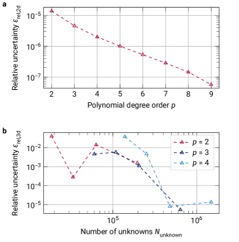
Figure S1: Relative numerical uncertainties $\epsilon_{\mathrm{rel}}$ of the simplified finite element model. a depicts the uncertainty depending on the polynomial degree order $p$ for the 2d case and constant $h$. b shows its dependence on different mesh discretizations $h$ for the 3d case and constant $p$. Smaller mesh discretizations $h$ lead to a larger number of unknowns $N_{\mathsf{unknown}}$ having to be determined. Dashed lines serve as guides to the eye.

To verify the convergence results considering a real Sawfish cavity, we calculate the quality factor $Q$ for a symmetric cavity with $N=$12$$ unit cells at either side of the cavity’s center and different finite element polynomial degrees $p$ (Fig. S2). In agreement with the parameter choice targeting $\epsilon_{\mathrm{rel,3d}}\approx$1\text{\times}{10}^{-5}$$, the quality factor stays constant for $p\geq$3$$.

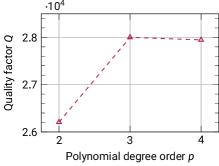
Figure S2: Dependence of a symmetric Sawfish cavity’s quality factor $Q$ with $N=$12$$ on the polynomial degree order $p$ in a 3d FEM simulation.

C.3 Cavity resonance estimation

Due to numerical uncertainties, the resonance frequencies of (symmetric and asymmetric) cavities deviate slightly from each other applying either the resonance problem or the scattering problem approach. We observe deviations up to approximately $10\text{\,}\mathrm{GHz}\text{/}$ in between both approaches. In the worst case and for high quality factors and thus narrow linewidths, a resonance frequency determined by the resonance problem approach is not resonant if the scattering problem approach is applied with that frequency.

To overcome this issue, we estimate the ‘scattering resonance frequency’ first for each scattering problem we are solving. At resonance, the electromagnetic energy flux through the waveguide of a waveguide-coupled cavity is highest. By solving the scattering problem for four dipole frequencies close to the expected resonance frequency, we obtain the frequency-dependent cavity transmission. Fitting the transmission with a Lorentzian function reveals the scattering resonance frequency (Fig. S3). This frequency is now used to recompute the respective scattering problem at resonance.

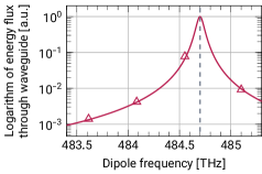
Figure S3: Exemplary Lorentzian fit of the frequency-dependent energy flux through the waveguide attached to a waveguide-coupled Sawfish cavity for estimating the ‘scattering resonance frequency’.

C.4 Dipole orientation

Diamond substrates cut along the crystallographic $\left[100\right]$ direction cause dipoles to enclose an angle of $\alpha=$54.7$^{\circ}$ with each cartesian axis ($\left[111\right]$ direction) [14, 15]. In turn, the dipoles do neither optimally overlap with the desired TM-like cavity mode nor with the modes of a rectangular waveguide attached to the cavity.

For a dipole embedded into a Sawfish cavity with parameters $N_{\mathrm{s}}=$23$$, $N_{\mathrm{w}}=$22$$, and $M=$19$$, we examine the dipole orientation’s influence by rotating the dipole within a plane spanned by the crystallographic $\left[111\right]$ ($\alpha=$54.7$^{\circ}$) and the $\left[010\right]$ ($\alpha=$0$^{\circ}$) direction (Fig. S4). The main article describes respective observations on $F_{\mathrm{P}}\left(\alpha\right)$ and on $\beta_{\mathrm{WG}}\left(\alpha\right)$. If the dipole is, for comparison, embedded into a plain waveguide with the rectangular cross section of the waveguide attached to the tapered Sawfish cavity, two aspects change as depicted in Fig. S4b. Firstly, the maximally achievable coupling efficiency is about $$86$\,\%$ (summing up the emission into both propagation directions). This proves that a cavity not only enhances the emission of an embedded dipole. It is furthermore a tool to couple light emitted by a dipole most efficiently to a guided waveguide mode by accurately designing the tapered interface between the cavity and the waveguide. Secondly, a plain waveguide is more susceptible to non-ideally oriented dipoles. For a dipole oriented along the $\left[111\right]$ direction in a plain waveguide, the waveguide coupling efficiency is decreased to $$66.3$\,\%$ of its ideal value.

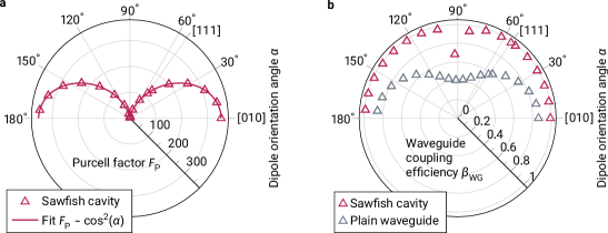
Figure S4: Dependence of the Purcell factor $F_{\mathrm{P}}$ and the waveguide coupling efficiency $\beta_{\mathrm{WG}}$ on the rotation angle $\alpha$ of a dipole being rotated within a plane defined by the crystallographic [010] and [111] directions for a Sawfish cavity with parameters $N_{\mathrm{s}}=$23$$, $N_{\mathrm{w}}=$22$$, and $M=$19$$. The dipole possesses a fixed emission frequency of $484.47\text{\,}\mathrm{THz}\text{/}$. For symmetry reasons, data in the range $180^{\circ}<\alpha\leq 360^{\circ}$ is not plotted. For comparison, b additionally shows the coupling efficiency of a dipole embedded into a plain, straight waveguide with the same rectangular cross section as the waveguide attached to the Sawfish cavity summing up the emission into both propagation directions (gray triangles).

C.5 Cavity-to-waveguide interface

To convert Bloch modes within the tapered cavity-to-waveguide interface into waveguide modes avoiding photon scattering, the cavity features have to taper off smoothly [16, 17]. The experimentally achievable minimal hole size is limited by fabrication constraints as sketched in Fig. S5. To date, elliptical holes’ minor axes of about $40\text{\,}\mathrm{nm}\text{/}$ in about $200\text{\,}\mathrm{nm}\text{/}$ thick diamond membranes have been reported [18, 19]. Thus, the arbitrary smooth conversion from Bloch to waveguide modes is not possible leading to increased scattering losses compared to the Sawfish design. Even if the corrugation features’ tips in our Sawfish design suffered from such fabrication uncertainties, this would likely not affect the interface’s performance since the electric field intensity is not localized at the tips (see cavity unit cells depicted in the main article).

Figure S5: Sketch of the established hole-based photonic crystal cavity design [20, 21, 22, 23]. Arbitrarily small hole-like features cannot be fabricated. Particularly, diameters of hole-like features are limited to $2r_{\mathrm{min}}$ within the cavity-to-waveguide interface.

C.6 Waveguide-to-fiber interface

The fiber-coupled Sawfish cavity also includes the well-established tapered waveguide-to-fiber interface [24], allowing us to quantify the total emitter-to-fiber interface efficiency $\eta$. To estimate the waveguide-to-fiber transmission $\beta_{\mathrm{F}}$, the waveguide’s fundamental mode is launched from the untapered part of the waveguide into the tapered direction. An (arbitrary) power is assigned to it. After propagating and transitioning into a fundamental fiber mode via an evanescent waveguide-fiber supermode (see main article), the mode overlap between the electric field arriving at a fiber cross section and the fundamental fiber mode is computed as a power ratio.

The effective refractive index of the transitioning optical mode is calculated at distinct cross sections of the 3d model employing propagating mode simulations performed with the software package JCMsuite [8]. Fig. S6 shows effective refractive indices along the waveguide-to-fiber interface. They accurately resemble the situation presented in [24] indicating an adiabatic transition.

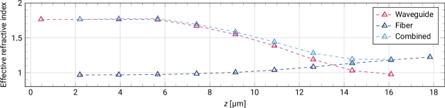
Figure S6: Effective refractive indices within the frame of an adiabatic waveguide-to-fiber interface as attached to the Sawfish cavity. Modes guided in the tapered waveguide are displayed in red, modes guided in the tapered fiber in dark blue, and modes of the combined system in light blue. Dashed lines serve as guides to the eye.

C.7 Bayesian optimization

The optimized structures presented in the main manuscript are obtained by means of a Bayesian optimization (BO) [25, 26] method. BO methods are sequential optimization methods that are very efficient at optimizing black box functions or processes that are expensive in terms of the consumed resources per evaluation [27]. In BO methods, a stochastic surrogate model, most often a Gaussian process (GP) [28], is trained on observations drawn from an expensive black box function $f(\bm{p})$, where $\bm{p}\in\mathcal{X}\subset\mathbb{R}^{N}$ and $f:\mathcal{X}\to\mathbb{R}$. After training, the GP serves as a stochastic predictor for the modeled function. In contrast to the modeled function itself, GPs are usually much faster to evaluate. Additionally, when compared to other machine learning methods such as deep neural networks [29, 30], the predictions made by a GP are usually easy to interpret [30]. This is due to the fact that the surrogate model’s hyperparameters directly relate to properties of the training data, like the mean, the variance, or the length scales on which the data changes. The GP’s predictions are used to iteratively generate new sample candidates $\bm{p}$ for evaluating the expensive model function. Sample candidates $\bm{p}$ are chosen to be effective for achieving the goal of the optimization, e.g. for finding the global minimum of the modeled function. The new values obtained from the expensive model retrain the GP. This continues until the optimization budget is exhausted.

As noted, GPs are a key component in BO methods. Being defined on the continuous domain $\mathcal{X}$, they extend finite-dimensional multivariate normal distributions (MVNs) to an infinite dimensional case [31]. Where MVNs are specified by a mean vector $\bm{\mu}$ and a positive (semi-)definite covariance matrix $\mathbf{\Sigma}$, GPs are completely specified by a mean function $\mu:\mathcal{X}\to\mathbb{R}$ and a covariance kernel function $k:\mathcal{X}\times\mathcal{X}\to\mathbb{R}$ [28]. We choose the commonly employed constant mean function and the Matérn $\nicefrac{{5}}{{2}}$ kernel function [32], i.e.

$$\begin{aligned} \mu(\bm{p})&=\mu_{0}\,,\\ k(\bm{p},\bm{p}^{\prime})&=\sigma_{0}\left(1+\sqrt{5}r+\frac{5}{3}r^{2}\right)\times\exp{\left(-\sqrt{5}r\right)}\,,\\ \end{aligned}$$ (20)

$$\text{where}\quad r=\sqrt{\sum_{i=1}^{N}\left(\frac{p_{i}-p^{\prime}_{i}}{l_{i}}\right)^{2}}\,.$$ (21)

The hyperparameters $\mu_{0}$ and $\sigma_{0}$, as well as the length scales $l_{1},\dots,l_{N}$, are selected to maximize the likelihood of the observations up to some maximum number of observations $W_{\mathrm{hyp}}$ [33]. Afterwards, only $\mu_{0}$ and $\sigma_{0}$ get updated. A GP that is trained on $W$ function values $\bm{Y}=\left[f(\bm{p}_{1}),\dots,f(\bm{p}_{W})\right]^{\mathrm{T}}$ allows to make predictions in the form of a normal distribution for each point $\bm{p}_{\ast}$ in the parameter space, i.e. it predicts function values

$$\hat{f}(\bm{p}_{\ast})\sim\mathcal{N}(\hat{y}(\bm{p}_{\ast}),\hat{\sigma}^{2}(\bm{p}_{\ast}))\,.$$

The values for the predicted mean $\hat{y}(\bm{p}_{\ast})$ and variance $\hat{\sigma}^{2}(\bm{p}_{\ast})$ are defined as

$$\hat{y}(\bm{p}_{\ast}) =\mu_{0}+\bm{k}^{\mathrm{T}}(\bm{p}_{\ast})\mathbf{K}^{-1}[\bm{Y}-\mu_{0}\bm{1}]\,,$$ (22)

$$\hat{\sigma}^{2}(\bm{p}_{\ast}) =\sigma_{0}^{2}-\bm{k}^{\mathrm{T}}(\bm{p}_{\ast})\mathbf{K}^{-1}\bm{k}(\bm{p}_{\ast})\,,$$ (23)

where $\bm{k}(\bm{p}_{\ast})=\left[k(\bm{p}_{\ast},\bm{p}_{1}),\dots,k(\bm{p}_{\ast},\bm{p}_{W})\right]^{\mathrm{T}}$ and $(\mathbf{K})_{ij}=k(\bm{p}_{i},\bm{p}_{j})$. For $\bm{p}_{\ast}$ very far from the explored regions, the predictions approach the prior mean and variance found during the hyperparameter optimization.

New sample candidates $\bm{p}_{W+1}$ are generated by selecting the parameter that maximizes some utility function $\alpha(\bm{p})$. Here, we consider the expected improvement (EI)  [27, 26, 31] with respect to the previously found smallest observed function value $f_{\mathrm{min}}\leavevmode\nobreak\ =\leavevmode\nobreak\ \min\{f(\bm{p}_{1}),\dots,f(\bm{p}_{W})\}$, i.e.

$$\bm{p}_{W+1}=\underset{\bm{p}\in\mathcal{X}}{\arg\max}\,\alpha_{\mathrm{EI}}(\bm{p})\,,$$ (24)

$$\text{where}\quad\alpha_{\mathrm{EI}}(\bm{p})=\mathrm{E}\left[\min\left(0,f_{\mathrm{min}}-\hat{f}(\bm{p})\right)\right]\,.$$ (25)

To perform the optimizations, we apply the analysis and optimization toolkit of the commercial finite element Maxwell solver JCMsuite [34, 35].

C.8 Impact of the fabrication tolerances and dipole displacements

By numerically optimizing the finite element models of the Sawfish cavity, we have obtained a set of parameters $\bm{p}_{\mathrm{opt}}$ that theoretically leads to peak performance, i.e. highest quality factors $Q$ or highest waveguide coupling efficiencies $\beta_{\mathrm{WG}}$. Imperfect manufacturing processes, though, give rise to deviations from the targeted ideal parameters. Thus, the actually realized parameters $\bm{p}_{\mathrm{realized}}$ scatter around $\bm{p}_{\mathrm{opt}}$ according to some probability distribution function (PDF) $\mathcal{F}$. This naturally has a negative impact on the expected performance of the manufactured device.

If the PDF of the manufacturing process $\mathcal{F}$ is known, the expected performance reduction can be quantified by means of Monte Carlo sampling techniques. In a naive approach, many samples from $\mathcal{F}$ are drawn and used to evaluate the finite element model $f(\bm{p})$. A statistical analysis of the finite element results provides insight into the expected performance reduction. However, the cost of a single evaluation of the full finite element model renders this approach infeasible.

Instead of using the actual finite element model function to perform the Monte Carlo sampling, we employ a surrogate model trained by machine learning based on Gaussian processes [28], as introduced in subsection C.7. Training is conducted on a comparatively small set of model parameters $\bm{P}_{\mathrm{train}}$ and associated finite element function values $f(\bm{P}_{\mathrm{train}})$. After training, the surrogate model serves as a cheap-to-evaluate interpolator $\hat{f}(\bm{p})$ for the actual finite element model. In [30] and [36], a GP surrogate model similarly replaces an expensive model function during Monte Carlo sampling.

C.8.1 Methodology

We assume that the parameters $\bm{p}_{\mathrm{realized}}$ realized by the manufacturing process are distributed according to a multivariate normal distribution (MVN) $\mathcal{F}=\mathcal{N}\left(\bm{\mu}_{\mathrm{device}},\mathbf{\Sigma}_{\mathrm{device}}\right)$, with mean $\bm{\mu}_{\mathrm{device}}$ and diagonal covariance matrix $\mathbf{\Sigma}_{\mathrm{device}}={\mathrm{diag}}\left(\sigma_{1}^{2},\dots,\sigma_{N}^{2}\right)$, i.e. $\bm{p}_{\mathrm{realized}}\sim\mathcal{F}$. The set $\left\{\sigma_{i}^{2}\right\}$ describes the variances of the individual manufacturing process parameters. By assuming diagonality, we imply that the outcome parameters are uncorrelated, i.e. that a parameter $p_{i}$ is not dependent on another parameter $p_{j}$.

The GP surrogate model is trained on a set of $W_{\mathrm{train}}$ training parameters $\bm{P}_{\mathrm{train}}=\{\bm{p}_{1},\dots,\bm{p}_{W_{\mathrm{train}}}\}$, that are used to evaluate the expensive finite element model $f(\bm{p})$ and to generate the training data $\bm{Y}=\{f(\bm{p}_{1}),\dots,f(\bm{p}_{W_{\mathrm{train}}})\}$. The training parameters are drawn from a training distribution $\mathcal{G}=\mathcal{N}\left(\bm{\mu}_{\mathrm{train}},\mathbf{\Sigma}_{\mathrm{train}}\right)$, with $\bm{\mu}_{\mathrm{train}}=\bm{\mu}_{\mathrm{device}}$ and $\mathbf{\Sigma}_{\mathrm{train}}=\kappa\times\mathbf{\Sigma}_{\mathrm{device}}$, where $\kappa>1$. Employing a MVN as a training distribution is advantageous since it favors the more regularly sampled locations close to the mean value of the manufacturing process distribution $\mathcal{F}$. As such, the region around $\bm{\mu}_{\mathrm{device}}$ is trained more intensely which promotes a small variance predicted by the GP surrogate. The available computational budget limits the total number of training samples $W_{\mathrm{train}}$. Mean values and variances predicted by the trained GP (c.f. subsection C.7) are then incorporated into the subsequent uncertainty impact analysis.

In a Monte Carlo sampling approach [37], we incrementally draw a large number of $N_{\mathrm{tot}}$ samples $\bm{P}_{\mathrm{sample}}=\{\bm{p}_{1},\dots,\bm{p}_{N_{\mathrm{tot}}}\}$ from the sampling distribution $\mathcal{H}=\mathcal{F}=\mathcal{N}\left(\bm{\mu}_{\mathrm{device}},\mathbf{\Sigma}_{\mathrm{device}}\right)$. For these sample parameters, the GP surrogate model is evaluated and the function values $\hat{y}(\bm{p})$ predicted for the finite element model as well as the associated variances $\hat{\sigma}^{2}(\bm{p})$ are calculated. Being dependent on random sample parameters, the predicted function values $\hat{\bm{Y}}_{\mathrm{tot}}=\{\hat{y}(\bm{p}_{1}),\dots,\hat{y}(\bm{p}_{N_{\mathrm{tot}}})\}\sim\mathcal{Q}$ are also random numbers that follow a statistical distribution $\mathcal{Q}$. The same holds for the predicted variance samples $\hat{\bm{S}}_{\mathrm{tot}}=\{\hat{\sigma}^{2}(\bm{p}_{1}),\dots,\hat{\sigma}^{2}(\bm{p}_{N_{\mathrm{tot}}})\}\sim\mathcal{R}$. Analyzing certain percentiles of the distribution $\mathcal{Q}$ allows to accurately quantify the impact of uncertainties in the manufacturing process. By further analyzing the distribution of the predicted variances $\mathcal{R}$, we infer an estimate of the uncertainty introduced by using a surrogate model instead of the expensive finite element model function.

For a Gaussian distribution, the $50$’th percentile describes the mean which equals the median. The $16$’th and $84$’th percentiles are tied to the lower and upper standard deviation, respectively. Accordingly, we investigate these percentiles of $\mathcal{Q}$ by analyzing the samples $\hat{\bm{Y}}_{\mathrm{tot}}$. The median $P_{50}(\hat{\bm{Y}}_{\mathrm{tot}})$ is given as the value for which we estimate a probability of $50\text{\,}\mathrm{\char 37\relax}\text{/}$ that the manufactured cavity will have at least this value. Lower and upper standard deviations are calculated as

$$\sigma_{-}(\hat{\bm{Y}}_{\mathrm{tot}}) =P_{50}(\hat{\bm{Y}}_{\mathrm{tot}})-P_{16}(\hat{\bm{Y}}_{\mathrm{tot}})\quad\text{and}$$ (26)

$$\sigma_{+}(\hat{\bm{Y}}_{\mathrm{tot}}) =P_{84}(\hat{\bm{Y}}_{\mathrm{tot}})-P_{50}(\hat{\bm{Y}}_{\mathrm{tot}})\,.$$ (27)

In order to quantify the uncertainty induced by using a surrogate model, we consider the $50$’th percentile of $\mathcal{R}$, i.e. $\sigma_{\mathrm{GP}}^{2}=P_{50}(\hat{\bm{S}}_{\mathrm{tot}})$. In contrast to ordinary Monte Carlo sampling, where the expectation value and its variance are calculated directly, our approach is capable of describing skewed distributions.

The error in Monte Carlo methods generally decreases as the number of samples increases. To estimate this error, we consider the Monte Carlo error for ordinary Monte Carlo sampling [38]

$$\sigma_{\mathrm{MC}}^{2}\approx\frac{\mathrm{Var}\left[\hat{\bm{Y}}_{\mathrm{tot}}\right]}{N_{\mathrm{tot}}}\,.$$ (28)

It requires the variance and in turn also the expectation value of the sample data $\hat{\bm{Y}}_{\mathrm{tot}}$, i.e.

$$\mathrm{Var}\left[\hat{\bm{Y}}_{\mathrm{tot}}\right]=\frac{1}{N_{\mathrm{tot}}}\sum_{i=1}^{N_{\mathrm{tot}}}\left(\hat{y}(\bm{p}_{i})-\mathrm{E}\left[\hat{\bm{Y}}_{\mathrm{tot}}\right]\right)^{2}$$ (29)

$$\text{and}\quad\mathrm{E}\left[\hat{\bm{Y}}_{\mathrm{tot}}\right]=\frac{1}{N_{\mathrm{tot}}}\sum_{i=1}^{N_{\mathrm{tot}}}\hat{y}(\bm{p}_{i})\,.$$ (30)

While the Monte Carlo error can be reduced by sampling the surrogate more often, the uncertainty introduced by the surrogate can only be reduced by increasing the number of training points $W_{\mathrm{train}}$. The Monte Carlo error and the surrogate uncertainty are combined into a compound uncertainty for the median

$$\sigma_{\mathrm{Median}}=\sqrt{\sigma_{\mathrm{MC}}^{2}+\sigma_{\mathrm{GP}}^{2}}\,.$$ (31)

The expected performance of the cavity is given in terms of these values, i.e.

$$\overline{f}=\left(P_{50}(\hat{\bm{Y}}_{\mathrm{tot}})\pm\sigma_{\mathrm{Median}}\right)^{\sigma_{+}(\hat{\bm{Y}}_{\mathrm{tot}})}_{\sigma_{-}(\hat{\bm{Y}}_{\mathrm{tot}})}\,.$$ (32)

Algorithm 1 outlines the complete procedure.

Algorithm 1 Determines the expected cavity performance for known manufacturing process uncertainties by means of Monte Carlo sampling of a trained Gaussian process surrogate model.

procedure MC simulation(Predicted GP mean $\hat{y}(\bm{p})$, predicted GP variance $\hat{\sigma}^{2}(\bm{p})$, sample distribution $\mathcal{H}$)

     $\sigma_{\mathrm{rel,MC}}\leftarrow\infty$ $\triangleright$ Relative MC error

     $\sigma_{\mathrm{lb}}\leftarrow$1\text{\times}{10}^{-3}$$ $\triangleright$ Lower error bound

     $N_{\mathrm{tot}}\leftarrow$0$$

     $\Delta N\leftarrow$1000$$ $\triangleright$ Sample increment

     $N_{\mathrm{min}}\leftarrow$50\,000$$ $\triangleright$ Minimum number of samples to be drawn

     $\hat{\bm{Y}}_{\mathrm{tot}}\leftarrow\emptyset$

     $\hat{\bm{S}}_{\mathrm{tot}}\leftarrow\emptyset$

     while $(\sigma_{\mathrm{rel,MC}}\geq\sigma_{\mathrm{lb}}$ and $N_{\mathrm{tot}}<N_{\mathrm{min}})$ do

         $\bm{P}_{\mathrm{sample}}\leftarrow$ draw $\Delta N$ samples from $\mathcal{H}$

         $\hat{\bm{Y}}\leftarrow\hat{y}(\bm{P}_{\mathrm{sample}})$

         $\hat{\bm{S}}\leftarrow\hat{\sigma}^{2}(\bm{P}_{\mathrm{sample}})$

         $\hat{\bm{Y}}_{\mathrm{tot}}\leftarrow\hat{\bm{Y}}_{\mathrm{tot}}\cup\hat{\bm{Y}}$

         $\hat{\bm{S}}_{\mathrm{tot}}\leftarrow\hat{\bm{S}}_{\mathrm{tot}}\cup\hat{\bm{S}}$

         $N_{\mathrm{tot}}\leftarrow N_{\mathrm{tot}}+\Delta N$

         Calculate $\sigma_{\mathrm{MC}}(\bm{Y}_{\mathrm{tot}})$ $\triangleright$ Equation 28

         $\sigma_{\mathrm{rel,MC}}(\bm{Y}_{\mathrm{tot}})\leftarrow\sigma_{\mathrm{MC}}(\bm{Y}_{\mathrm{tot}})/P_{50}(\bm{Y}_{\mathrm{tot}})$

     end while

     $\sigma_{\mathrm{GP}}^{2}\leftarrow P_{50}(\hat{\bm{S}}_{\mathrm{tot}})$

     $\sigma_{\mathrm{Median}}\leftarrow\sqrt{\sigma_{\mathrm{GP}}^{2}+\sigma_{\mathrm{MC}}^{2}}$

     $\sigma_{+}(\bm{Y}_{\mathrm{tot}})\leftarrow P_{84}(\bm{Y}_{\mathrm{tot}})-P_{50}(\bm{Y}_{\mathrm{tot}})$

     $\sigma_{-}(\bm{Y}_{\mathrm{tot}})\leftarrow P_{50}(\bm{Y}_{\mathrm{tot}})-P_{16}(\bm{Y}_{\mathrm{tot}})$

     return $\left(P_{50}(\hat{\bm{Y}}_{\mathrm{tot}})\pm\sigma_{\mathrm{Median}}\right)^{\sigma_{+}(\hat{\bm{Y}}_{\mathrm{tot}})}_{\sigma_{-}(\hat{\bm{Y}}_{\mathrm{tot}})}$

end procedure

C.8.2 Impact of dipole displacements

The exact position of the dipole emitter within the cavity impacts the expected Purcell factor $F_{\mathrm{P}}$ and the waveguide coupling efficiency $\beta_{\mathrm{WG}}$. To quantify the position’s influence, the method introduced in subsubsection C.8.1 is applied. For the manufacturing process distribution, it is assumed that the placement of the dipole can be achieved with a standard deviation of $25\text{\,}\mathrm{nm}\text{/}$ in each cartesian direction around the cavity’s center. A training dataset with $209$ data points $\bm{P}_{\mathrm{train}}\sim\mathcal{N}(\bm{\mu}_{\mathrm{train}},\mathbf{\Sigma}_{\mathrm{train}})$ is generated. Here, $\bm{\mu}_{\mathrm{train}}=\bm{0}$ and $\mathbf{\Sigma}_{\mathrm{train}}={\mathrm{diag}}($35\text{\,}\mathrm{nm}\text{/}$,$35\text{\,}\mathrm{nm}\text{/}$,$35\text{\,}\mathrm{nm}\text{/}$)^{2}$, i.e. relying on a standard deviation of $35\text{\,}\mathrm{nm}\text{/}$ in each cartesian direction, the training dataset encloses the assumed placement distribution. The expensive finite element model function is evaluated using $\bm{P}_{\mathrm{train}}$. Five training parameters in $\bm{P}_{\mathrm{train}}$ are removed since their results deviate strongly from the local average over adjacent samples. The GP surrogate now originates from the $204$ remaining training parameters and results.

Accordingly, the sampling parameters $\bm{P}_{\mathrm{sample}}$ to evaluate the GP surrogates in the Monte Carlo sampling approach are drawn from a MVN with $\bm{\mu}_{\mathrm{sample}}=\bm{0}$ and $\mathbf{\Sigma}_{\mathrm{sample}}={\mathrm{diag}}($25\text{\,}\mathrm{nm}\text{/}$,$25\text{\,}\mathrm{nm}\text{/}$,$25\text{\,}\mathrm{nm}\text{/}$)^{2}$. Fig. S7 depicts the distributions of the predicted Purcell factor $F_{\mathrm{P}}$ and the waveguide coupling efficiency $\beta_{\mathrm{WG}}$.

For the Purcell factor $F_{\mathrm{P}}$, we predict a value of

$$\overline{F}_{\mathrm{P}}=\left($91.4$\pm$3.2$\right)^{+$18.3$}_{-$26.0$}\,,$$

where the standard deviation of the median $\sigma_{\mathrm{Median}}$ consists of the surrogate uncertainty $\sigma_{\mathrm{GP}}=$3.2$$ and the numerical Monte Carlo error $\sigma_{\mathrm{MC}}=$0.1$$. Likewise, we obtain $\beta_{\mathrm{WG}}$

$$\overline{\beta}_{\mathrm{WG}}=\left($0.9863$\pm$0.0014$\right)^{+$0.0003$}_{-$0.0014$}\,,$$

where the standard deviation of the median $\sigma_{\mathrm{Median}}$ consists of the surrogate uncertainty $\sigma_{\mathrm{GP}}=$0.0014$$ and the numerical Monte Carlo error $\sigma_{\mathrm{MC}}=$0.0001$$.

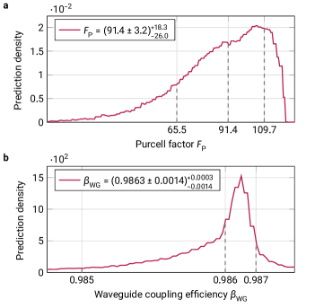
Figure S7: Expected cavity performance regarding the Purcell factor $F_{\mathrm{P}}$ a and the waveguide coupling efficiency $\beta_{\mathrm{WG}}$ b for dipoles displaced according to a manufacturing process distribution $\mathcal{F}$. The values given on the abscissa relate to the respective median minus standard deviation, median, and median plus standard deviation.

C.8.3 Impact of fabrication tolerances

Similarly, the exact geometry of the manufactured cavity affects the expected Purcell factor $F_{\mathrm{P}}$ and the waveguide coupling efficiency $\beta_{\mathrm{WG}}$. For the manufacturing process distribution, we assume fabrication parameters scattered around a desired mean value of $\bm{p}_{\mathrm{opt}}=\left[\Delta T,\allowbreak{}\delta,\allowbreak{}\Delta g\right]=\left[$0\text{\,}\mathrm{nm}\text{/}$,\allowbreak{}$90\text{\,}\mathrm{\SIUnitSymbolDegree}\text{/}$,\allowbreak{}$0\text{\,}\mathrm{nm}\text{/}$\right]$ with uncertainties $\mathbf{\Sigma}_{\mathrm{sample}}={\mathrm{diag}}($0.8\text{\,}\mathrm{nm}\text{/}$,$0.1\text{\,}\mathrm{\SIUnitSymbolDegree}\text{/}$,$0.8\text{\,}\mathrm{nm}\text{/}$)^{2}$. A training dataset consisting of $349$ data points $\bm{P}_{\mathrm{train}}\sim\mathcal{N}(\bm{\mu}_{\mathrm{train}},\mathbf{\Sigma}_{\mathrm{train}})$ is produced. Here, $\bm{\mu}_{\mathrm{train}}=\bm{p}_{\mathrm{opt}}$ and $\mathbf{\Sigma}_{\mathrm{train}}={\mathrm{diag}}($3.75\text{\,}\mathrm{nm}\text{/}$,$1.35\text{\,}\mathrm{\SIUnitSymbolDegree}\text{/}$,$3.75\text{\,}\mathrm{nm}\text{/}$)^{2}$, i.e. we select a training distribution which encloses the assumed manufacturing process distribution. The expensive finite element model function is evaluated using $\bm{P}_{\mathrm{train}}$ to train the GP surrogate models, excluding $74$ samples for which the resonance frequency could not be determined according to subsection C.3.

The sampling parameters $\bm{P}_{\mathrm{sample}}$ to evaluate the GP surrogates in the Monte Carlo sampling approach are drawn from a MVN with $\bm{\mu}_{\mathrm{sample}}=\bm{p}_{\mathrm{opt}}$ and $\mathbf{\Sigma}_{\mathrm{sample}}={\mathrm{diag}}($0.8\text{\,}\mathrm{nm}\text{/}$,$0.1\text{\,}\mathrm{\SIUnitSymbolDegree}\text{/}$,$0.8\text{\,}\mathrm{nm}\text{/}$)^{2}$. Sampling parameters for which the surrogate evaluation leads to $F_{\mathrm{P}}\leq$1$$ are excluded from the calculation of the predicted values since they describe nonresonant (thus defective) cavities. The amount of samples discarded by this criterion is below $$5$\,\%$. Fig. S8 displays the distributions of the predicted Purcell factor $F_{\mathrm{P}}$ and the waveguide coupling efficiency $\beta_{\mathrm{WG}}$.

For the Purcell factor $F_{\mathrm{P}}$, this yields a predicted value of

$$\overline{F}_{\mathrm{P}}=\left($48.5$\pm$26.5$\right)^{+$48.0$}_{-$33.5$}\,,$$

where the standard deviation of the median $\sigma_{\mathrm{Median}}$ consists of the surrogate uncertainty $\sigma_{\mathrm{GP}}=$26.5$$ and the numerical Monte Carlo error $\sigma_{\mathrm{MC}}=$0.1$$. Likewise, it is

$$\overline{\beta}_{\mathrm{WG}}=\left($0.929$\pm$0.054$\right)^{+$0.057$}_{-$0.141$}\,,$$

where the standard deviation of the median $\sigma_{\mathrm{Median}}$ consists of the surrogate uncertainty $\sigma_{\mathrm{GP}}=$0.054$$ and the numerical Monte Carlo error $\sigma_{\mathrm{MC}}=$0.001$$.

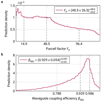
Figure S8: Expected cavity performance regarding the Purcell factor $F_{\mathrm{P}}$ a and the waveguide coupling efficiency $\beta_{\mathrm{WG}}$ b for fabrication (geometry) parameters distributed according to a manufacturing process distribution $\mathcal{F}$. The values given on the abscissa relate to the respective median minus standard deviation, median, and median plus standard deviation.

References

- [1] Carlo Bradac, Weibo Gao, Jacopo Forneris, Matthew E. Trusheim and Igor Aharonovich “Quantum nanophotonics with group IV defects in diamond” In Nat. Commun. 10.5625 Springer ScienceBusiness Media LLC, 2019 DOI: 10.1038/s41467-019-13332-w
- [2] Matthew E. Trusheim et al. “Transform-Limited Photons From a Coherent Tin-Vacancy Spin in Diamond” In Phys. Rev. Lett. 124.023602 American Physical Society (APS), 2020 DOI: 10.1103/physrevlett.124.023602
- [3] Marcus W. Doherty et al. “The nitrogen-vacancy colour centre in diamond” In Phys. Rep. 528 Elsevier BV, 2013, pp. 1–45 DOI: 10.1016/j.physrep.2013.02.001
- [4] Ph. Tamarat et al. “Stark Shift Control of Single Optical Centers in Diamond” In Phys. Rev. Lett. 97.083002 American Physical Society (APS), 2006 DOI: 10.1103/physrevlett.97.083002
- [5] Johannes Borregaard et al. “One-Way Quantum Repeater Based on Near-Deterministic Photon-Emitter Interfaces” In Phys. Rev. X 10.021071 American Physical Society (APS), 2020 DOI: 10.1103/physrevx.10.021071
- [6] Valerio Scarani et al. “The security of practical quantum key distribution” In Rev. Modern Phys. 81.1301 American Physical Society (APS), 2009 DOI: 10.1103/revmodphys.81.1301
- [7] J. Chang et al. “Detecting telecom single photons with % system detection efficiency and high time resolution” In APL Photonics 6.036114 AIP Publishing, 2021 DOI: 10.1063/5.0039772
- [8] “JCMsuite”
- [9] Chiu-Yen Kao and Fadil Santosa “Maximization of the quality factor of an optical resonator” In Wave Motion 45.4 Elsevier BV, 2008, pp. 412–427 DOI: 10.1016/j.wavemoti.2007.07.012
- [10] Jelena Vučković, Marko Lončar, Hideo Mabuchi and Axel Scherer “Design of photonic crystal microcavities for cavity QED” In Phys. Rev. E 65.016608 American Physical Society (APS), 2001 DOI: 10.1103/physreve.65.016608
- [11] E.. Purcell “Spontaneous Emission Probabilities at Radio Frequencies” In Proceedings of the American Physical Society 69.11-12 American Physical Society (APS), 1946, pp. 674–674 DOI: 10.1103/physrev.69.674
- [12] Jan Pomplun, Sven Burger, Lin Zschiedrich and Frank Schmidt “Adaptive finite element method for simulation of optical nano structures” In physica status solidi (b) 244 Wiley Online Library, 2007, pp. 3419–3434
- [13] Maria Rozova, Jan Pomplun, Lin Zschiedrich, Frank Schmidt and Sven Burger “3D finite element simulation of optical modes in VCSELs” In Physics and Simulation of Optoelectronic Devices XX 8255 SPIE, 2012, pp. 129–136 International Society for OpticsPhotonics DOI: 10.1117/12.906372
- [14] Christian Hepp et al. “Electronic Structure of the Silicon Vacancy Color Center in Diamond” In Phys. Rev. Lett. 112.036405 American Physical Society (APS), 2014 DOI: 10.1103/physrevlett.112.036405
- [15] Johannes Görlitz et al. “Spectroscopic investigations of negatively charged tin-vacancy centres in diamond” In New J. Phys. 22.013048 IOP Publishing, 2020 DOI: 10.1088/1367-2630/ab6631
- [16] M. Palamaru and Ph. Lalanne “Photonic crystal waveguides: Out-of-plane losses and adiabatic modal conversion” In Appl. Phys. Lett. 78.1466 AIP Publishing, 2001 DOI: 10.1063/1.1354666
- [17] C. Sauvan, G. Lecamp, P. Lalanne and J.. Hugonin “Modal-reflectivity enhancement by geometry tuning in Photonic Crystal microcavities” In Opt. Express 13 The Optical Society, 2005, pp. 245–255 DOI: 10.1364/opex.13.000245
- [18] Michael J. Burek et al. “Fiber-Coupled Diamond Quantum Nanophotonic Interface” In Phys. Rev. Appl. 8.024026 American Physical Society (APS), 2017 DOI: 10.1103/physrevapplied.8.024026
- [19] E.. Knall et al. “Efficient Source of Shaped Single Photons Based on an Integrated Diamond Nanophotonic System” In Phys. Rev. Lett. 129.053603 American Physical Society (APS), 2022 DOI: 10.1103/physrevlett.129.053603
- [20] Sara Mouradian, Noel H. Wan, Tim Schröder and Dirk Englund “Rectangular photonic crystal nanobeam cavities in bulk diamond” In Appl. Phys. Lett. 111.021103 AIP Publishing, 2017 DOI: 10.1063/1.4992118
- [21] R.. Evans et al. “Photon-mediated interactions between quantum emitters in a diamond nanocavity” In Science 362.6415 American Association for the Advancement of Science (AAAS), 2018, pp. 662–665 DOI: 10.1126/science.aau4691
- [22] Alison E. Rugar et al. “Quantum Photonic Interface for Tin-Vacancy Centers in Diamond” In Phys. Rev. X 11.031021 American Physical Society (APS), 2021 DOI: 10.1103/physrevx.11.031021
- [23] Kazuhiro Kuruma et al. “Coupling of a single tin-vacancy center to a photonic crystal cavity in diamond” In Appl. Phys. Lett. 118.230601 AIP Publishing, 2021 DOI: 10.1063/5.0051675
- [24] T.. Tiecke et al. “Efficient fiber-optical interface for nanophotonic devices” In Optica 2.2 The Optical Society, 2015, pp. 70–75 DOI: 10.1364/optica.2.000070
- [25] Jonas Močkus “On Bayesian methods for seeking the extremum” In Optimization techniques IFIP technical conference Springer, 1975, pp. 400–404
- [26] Jonas Močkus “Bayesian approach to global optimization: theory and applications” Springer Science & Business Media, 2012
- [27] Donald R. Jones, Matthias Schonlau and William J. Welch “Efficient global optimization of expensive black-box functions” In J. Global Optim. 13 Springer, 1998, pp. 455–492
- [28] Christopher K. Williams and Carl Edward Rasmussen “Gaussian processes for machine learning” MIT Press, 2006
- [29] Grégoire Montavon, Wojciech Samek and Klaus-Robert Müller “Methods for interpreting and understanding deep neural networks” In Digit. Signal Process. 73 Elsevier BV, 2018, pp. 1–15 DOI: 10.1016/j.dsp.2017.10.011
- [30] Carl Edward Rasmussen “Gaussian Processes to Speed up Hybrid Monte Carlo for Expensive Bayesian Integrals” In Bayesian Statistics 7 Oxford University Press, 2003, pp. 651–659
- [31] Roman Garnett “Bayesian Optimization” in preparation Cambridge University Press, 2022 URL: https://bayesoptbook.com/
- [32] Eric Brochu, Vlad M. Cora and Nando Freitas “A Tutorial on Bayesian Optimization of Expensive Cost Functions, with Application to Active User Modeling and Hierarchical Reinforcement Learning”, 2010 arXiv:1012.2599 [cs.LG]
- [33] Xavier Garcia-Santiago, Philipp-Immanuel Schneider, Carsten Rockstuhl and Sven Burger “Shape design of a reflecting surface using Bayesian Optimization” In Journal of Physics: Conference Series 963.012003, 2018 IOP Publishing
- [34] Philipp-Immanuel Schneider et al. “Benchmarking five global optimization approaches for nano-optical shape optimization and parameter reconstruction” In ACS Photonics 6.11 ACS Publications, 2019, pp. 2726–2733
- [35] Philipp-Immanuel Schneider, Martin Hammerschmidt, Lin Zschiedrich and Sven Burger “Using Gaussian process regression for efficient parameter reconstruction” In Metrology, Inspection, and Process Control for Microlithography XXXIII 10959 SPIE, 2019, pp. 200–207 International Society for OpticsPhotonics DOI: 10.1117/12.2513268
- [36] Matthias Plock, Kas Andrle, Sven Burger and Philipp-Immanuel Schneider “Bayesian Target-Vector Optimization for Efficient Parameter Reconstruction” In Adv. Theory Simul. Wiley, 2022, pp. 2200112 DOI: 10.1002/adts.202200112
- [37] Christian P. Robert and George Casella “Monte Carlo Statistical Methods” Springer, 2004
- [38] Kevin P. Murphy “Machine learning: a probabilistic perspective” MIT Press, 2012