Calibrating AI Models for Few-Shot Demodulation via Conformal Prediction

Abstract

AI tools can be useful to address model deficits in the design of communication systems. However, conventional learning-based AI algorithms yield poorly calibrated decisions, unabling to quantify their outputs uncertainty. While Bayesian learning can enhance calibration by capturing epistemic uncertainty caused by limited data availability, formal calibration guarantees only hold under strong assumptions about the ground-truth, unknown, data generation mechanism. We propose to leverage the conformal prediction framework to obtain data-driven set predictions whose calibration properties hold irrespective of the data distribution. Specifically, we investigate the design of baseband demodulators in the presence of hard-to-model nonlinearities such as hardware imperfections, and propose set-based demodulators based on conformal prediction. Numerical results confirm the theoretical validity of the proposed demodulators, and bring insights into their average prediction set size efficiency.

Index Terms—  Calibration, Conformal Prediction, Demodulation

1 Introduction

Artificial intelligence (AI) models typically report a confidence measure associated with each prediction, which reflects the model’s self-evaluation of the accuracy of a decision. Notably, neural networks implement probabilistic predictors that produce a probability distribution across all possible values of the output variable. As an example, Fig. 1 illustrates the operation of a neural network-based demodulator [1, 2, 3], which outputs a probability distribution on the constellation points given the corresponding received baseband sample. The self-reported model confidence, however, may not be a reliable measure of the true, unknown, accuracy of the prediction, in which case we say that the AI model is poorly calibrated. Poor calibration may be a substantial problem when AI-based decisions are processed within a larger system such as a communication network.

Deep learning models tend to produce either overconfident decisions when designed following a frequentist framework [4]; or else calibration levels that rely on strong assumptions about the ground-truth, unknown, data generation mechanism when Bayesian learning is applied [5, 6, 7, 8, 9, 10]. This paper investigates the adoption of conformal prediction (CP) [11, 12, 13] as a framework to design provably well-calibrated AI predictors, with distribution-free calibration guarantees that do not require making any assumption about the ground-truth data generation mechanism.

[width=8.5cm]Figs/fig_tikz_qpsk_prob_pred

Fig. 1: QPSK demodulation with a demodulator trained using a limited number of pilots (gray symbols): (a) Constellation symbols (colored markers), optimal hard prediction (dashed lines), and model trained using the few pilots (solid lines). Accuracy and calibration of the trained predictor depend on the test input (gray square). (b) Probabilistic predictors obtained from the trained model (solid bars) and optimal predictive probabilities (dashed bars), with thick line indicating the hard prediction. (c) Set predictors output a subset of the constellation symbols for each input.

Consider again the example in Fig. 1, which corresponds to the problem of designing a demodulator for a QPSK constellation in the presence of an I/Q imbalance that rotates and distorts the constellation. The hard decision regions of an optimal demodulator and of a data-driven demodulator trained on few pilots are displayed in panel (a), while the corresponding probabilistic predictions for some outputs are shown in panel (b). Depending on the input, the trained probabilistic model may result in either accurate or inaccurate hard predictions, whose accuracy is correctly or incorrectly characterized, resulting in well-calibrated or poorly calibrated predictions. Note that a well-calibrated probabilistic predictor should provide output probabilities close to the optimal predictor (dashed lines in panel (b)). Importantly, accuracy and calibration are distinct requirements.

CP leverages probabilistic predictors as a starting point to construct well-calibrated set predictors. Instead of producing a probability vector (as in Fig. 1(b)), a set predictor outputs a subset of the output space (see Fig. 1(c)). A set predictor is well-calibrated if it contains the correct output with a pre-defined probability selected by the system designer. This paper introduces CP-based demodulators, obtaining set predictors that satisfy formal calibration guarantees that hold irrespective of the ground-truth, unknown, distribution. The proposed approach is particularly relevant in practical situations characterized by a limited number of pilots, in which characterizing uncertainty is of critical importance.

In the rest of the paper, we first define the problem and present preliminaries in Sec. 2. Then, we introduce CP-based set predictors in Sec. 3, and describe experiments and conclusions in Sec. 4.

2 Problem Definition

2.1 Channel Model

Following the example in Fig. 1, we consider a communication link subject to phase fading and to unknown hardware distortions at the transmitter side [1, 14]. Our goal is to design a well-calibrated data-driven set demodulator based on the observation of a few pilots. We follow the unconventional notation of denoting as $y[i]$ the $i$-th transmitted symbol, and as $x[i]$ the corresponding received sample. This will allow us to write expressions for the demodulator in a more familiar way, with $x$ representing the input and $y$ the output. Each frame consists of $N$ pilots symbols and data symbols. The pilots define a data set ${\mathcal{D}}=\{z[i]\}_{i=1}^{N}$ of $N$ examples of input-output pairs $z[i]=(x[i],y[i])$ for $i=1,\ldots,N$, which is available to the receiver for the design of the demodulator.

Each transmitted symbol $y[i]$ is drawn uniformly at random from a given constellation $\mathcal{Y}$ [15]. For any given frame, the received sample $x[i]$ can be written as

$${\mathbf{x}}[i]=e^{\jmath{\boldsymbol{\psi}}}f_{\text{IQ}}({\mathbf{y}}[i])+{\mathbf{v}}[i],$$ (1)

for a random phase ${\boldsymbol{\psi}}\sim\mathrm{U}[0,2\pi)$, where the additive noise is ${\mathbf{v}}[i]\sim\mathcal{CN}(0,\mathrm{SNR}^{-1})$ for a given signal-to-noise ratio level $\mathrm{SNR}$. Furthermore, the I/Q imbalance function [16] is

$$f_{\text{IQ}}({\mathbf{y}}[i])=\bar{{\mathbf{y}}}_{\text{I}}[i]+\jmath\bar{{\mathbf{y}}}_{\text{Q}}[i],$$ (2)

where

$$\begin{bmatrix}\bar{{\mathbf{y}}}_{\text{I}}[i]\\ \bar{{\mathbf{y}}}_{\text{Q}}[i]\end{bmatrix}=\begin{bmatrix}1+{\boldsymbol{\epsilon}}&0\\ 0&1-{\boldsymbol{\epsilon}}\end{bmatrix}\begin{bmatrix}\cos{\boldsymbol{\delta}}&-\sin{\boldsymbol{\delta}}\\ -\sin{\boldsymbol{\delta}}&\cos{\boldsymbol{\delta}}\end{bmatrix}\begin{bmatrix}{\mathbf{y}}_{\text{I}}[i]\\ {\mathbf{y}}_{\text{Q}}[i]\end{bmatrix},$$ (3)

with ${\mathbf{y}}_{\text{I}}[i]$ and ${\mathbf{y}}_{\text{Q}}[i]$ being the real and imaginary parts of the modulated symbol ${\mathbf{y}}[i]$; and $\bar{{\mathbf{y}}}_{\text{I}}[i]$ and $\bar{{\mathbf{y}}}_{\text{Q}}[i]$ standing for the real and imaginary parts of the transmitted symbol $f_{\text{IQ}}({\mathbf{y}}[i])$. The channel parameters ${\boldsymbol{\psi}}$, ${\boldsymbol{\epsilon}}$, and ${\boldsymbol{\delta}}$ are generated independently in each frame from a common distribution.

2.2 Probabilistic Predictors

Probabilistic predictors implement a parametric conditional distribution model $p(y|x,\phi)$ on the output $y\in\mathcal{Y}$ given the input $x\in\mathcal{X}$, where $\phi\in\Phi$ is a vector of model parameters. Given the training data set ${\mathcal{D}}$ consisting of the $N$ pilots in a frame, frequentist learning produces an optimized single vector $\phi_{\mathcal{D}}^{*}$, while Bayesian learning returns a distribution $q^{*}(\phi|{\mathcal{D}})$ on the model parameter space $\Phi$ [17, 18]. We denote as $p(y|x,{\mathcal{D}})$ the resulting optimized predictive distribution which is either $p(y|x,\phi_{{\mathcal{D}}}^{*})$ for frequentist learning, or the ensemble $\mathrm{E}_{{\boldsymbol{\phi}}\sim q^{*}(\phi|{\mathcal{D}})}[p(y|x,{\boldsymbol{\phi}})]$ for Bayesian learning.

2.3 Set Predictors

A set predictor is defined as a set-valued function $\Gamma(\cdot|{\mathcal{D}}):\mathcal{X}~{}\rightarrow~{}2^{\mathcal{Y}}$ that maps an input $x$ to a subset of the output domain $\mathcal{Y}$ based on data set ${\mathcal{D}}$. We denote the size of the set predictor for input $x$ as $|\Gamma(x|{\mathcal{D}})|$. As illustrated in the example of Fig. 1, it depends in general on input $x$, and can be taken as a measure of the uncertainty of the set predictor.

The performance of a set predictor is evaluated in terms of coverage and inefficiency. Coverage refers to the probability that the true label is included in the predicted set; while inefficiency refers to the average size $|\Gamma(x|{\mathcal{D}})|$ of the predicted set. There is clearly a trade-off between two metrics.

Formally, the coverage level of set predictor $\Gamma$ is the probability that the true output $y$ is included in the prediction set $\Gamma(x|{\mathcal{D}})$ for a test pair $z=(x,y)$. This can be expressed as $\mathrm{coverage}(\Gamma)~{}=\mathbb{P}~{}\big{(}{\mathbf{y}}\in\Gamma({\mathbf{x}}|\mathbfcal{D})\big{)}$, where the probability $\mathbb{P}(\cdot)$ is taken over the ground-truth joint distribution of the involved random variables. When setting as target design a miscoverage level $\alpha\in[0,1]$, the set predictor $\Gamma$ is said to be $1-\alpha$-valid if

$$\mathrm{coverage}(\Gamma)=\mathbb{P}\big{(}{\mathbf{y}}\in\Gamma({\mathbf{x}}|\mathbfcal{D})\big{)}\geq 1-\alpha.$$ (4)

It is straightforward to design a valid set predictors even for the restrictive case of miscoverage level $\alpha=0$ by producing the full set $\Gamma(x|{\mathcal{D}})=\mathcal{Y}$ for all inputs $x$. One should, therefore, also consider the inefficiency of predictor $\Gamma$. The inefficiency of set predictor $\Gamma$ is defined as the average predictive set size

$$\mathrm{inefficiency}(\Gamma)=\mathrm{E}\Big{[}\big{|}\Gamma({\mathbf{x}}|\mathbfcal{D})\big{|}\Big{]},$$ (5)

where the average is taken over the data set ${\mathbfcal{D}}$ and the test pair $({\mathbf{x}},{\mathbf{y}})$ following their exchangeable joint distribution $p_{0}({\mathcal{D}},(x,y))$.

We note that the coverage condition (4) is practically relevant if the learner produces multiple predictions using independent data set ${\mathcal{D}}$, and is tested on multiple pairs $(x,y)$. In fact, in this case, the probability in (4) can be interpreted as the fraction of predictions for which the set predictor $\Gamma(x|{\mathcal{D}})$ includes the correct output. This situation reflects well the setting of interest in which a different demodulator is designed for each frame.

2.4 Naïve Set Predictors from Probabilistic Predictors

Given a probabilistic predictor $p(y|x,{\mathcal{D}})$, one can construct a set predictor by relying on the confidence levels reported by the model. To this end, one can construct the smallest subset of the output domain $\mathcal{Y}$ that covers a fraction $1-\alpha$ of the probability designed by model $p(y|x,{\mathcal{D}})$ given an input $x$. Given that probabilistic predictors are typically poorly calibrated, this approach generally does not satisfy condition (4) for the given desired miscoverage level $\alpha$.

3 Conformal Prediction

3.1 Nonconformity Scores

Conformal prediction relies on some form of validation to calibrate a naïve predictor. For any given test input $x$, a value $y^{\prime}\in\mathcal{Y}$ for input $x$ is included in the prediction set if $(x,y^{\prime})$ “conforms” well with the validation data. To formalize CP, we define a nonconformity (NC) score as a function that maps a pair $z=(x,y)$ and a data set ${\mathcal{D}}$ with $N$ samples to a real number, measuring how dissimilar the data point $z$ is to the data points in the fitting data set ${\mathcal{D}}$. An NC score must be invariant to permutations of the samples in the data set ${\mathcal{D}}$.

Given a trained probabilistic model $p(y|x,{\mathcal{D}})$, which may be frequentist or Bayesian, an NC score can be obtained as the log-loss

$${\mathrm{NC}}(z=(x,y)|{\mathcal{D}})=-\log p(y|x,{\mathcal{D}})$$ (6)

as long as the training algorithm used to derive the predictor $p(y|x,{\mathcal{D}})$ is invariant to permutations of the data set ${\mathcal{D}}$. Note that (6) measures how poorly the sample $(x,y)$ conforms with respect to the data set ${\mathcal{D}}$ via the trained model $p(y|x,{\mathcal{D}})$: If the sample $(x,y)$ is “similar” to the points in the set ${\mathcal{D}}$, the log-loss will tend to be small.

3.2 Validation-Based Set Predictors

Validation-based (VB)-CP set predictors partition the available set ${\mathcal{D}}={\mathcal{D}^{\text{tr}}}\cup{\mathcal{D}^{\text{val}}}$ into training set ${\mathcal{D}^{\text{tr}}}$ with ${N^{\text{tr}}}$ samples and a validation set ${\mathcal{D}^{\text{val}}}$ with ${N^{\text{val}}}=N-{N^{\text{tr}}}$ samples.

Given a test input $x$, for each candidate output $y^{\prime}$ in $\mathcal{Y}$, the NC score ${\mathrm{NC}}((x,y^{\prime})|{\mathcal{D}^{\text{tr}}})$ is evaluated by using the training data ${\mathcal{D}^{\text{tr}}}$. The NC score ${\mathrm{NC}}((x,y^{\prime})|{\mathcal{D}^{\text{tr}}})$ is compared to the NC scores ${\mathrm{NC}}(z^{\text{val}}[i]|{\mathcal{D}^{\text{tr}}})$ evaluated on all points $z^{\text{val}}[i],i=1,\dots,{N^{\text{val}}}$ in the validation set ${\mathcal{D}^{\text{val}}}$. If the pair $(x,y^{\prime})$ has a lower (or equal) NC score than a portion of at least $\lfloor\alpha(N^{\text{val}}+1)\rfloor/N^{\text{val}}$ of the validation NC scores, then the candidate label $y^{\prime}$ is included in the VB prediction set $\Gamma_{\alpha}^{\text{VB}}(x|{\mathcal{D}})$. Accordingly, the VB-CP set predictor is obtained as

$$\Gamma_{\alpha}^{\text{VB}}(x|{\mathcal{D}})=\Big{\{}y^{\prime}\in\mathcal{Y}\Big{|}\!\!\!\!\!\! {\mathrm{NC}}((x,y^{\prime})|{\mathcal{D}^{\text{tr}}})$$

$$\leq{Q}_{1-\alpha}\big{(}\{{\mathrm{NC}}(z^{\text{val}}[i]|{\mathcal{D}^{\text{tr}}})\}_{i=1}^{N^{\text{val}}}\big{)}\Big{\}}.$$

where the $(1-\alpha)$-empirical quantile ${Q}_{1-\alpha}\ \big{(}\{r[i]\}_{i=1}^{N}\big{)}$ for a set of $N$ real values $\{r[i]\}_{i=1}^{N}$ is the $\big{\lceil}(1-\alpha)(N+1)\big{\rceil}$ th smallest value of the set $\{r[i]\}_{i=1}^{N}\cup\{+\infty\}$.

It is known from [11] that the VB-CP set predictor satisfies the coverage condition (4). In terms of computational complexity, given ${N^{\text{te}}}$ test inputs, predictor $p(y|x,{\mathcal{D}})$ should be trained only once based on the training set ${\mathcal{D}^{\text{tr}}}$. This is followed by ${N^{\text{te}}}|\mathcal{Y}|+N^{\text{val}}$ evaluations of the NC scores to obtain the ${N^{\text{te}}}$ set predictions for all test points.

3.3 Cross-Validation-Based Set Predictors

VB-CP has the computational advantage of requiring a single training step, but the split into training and validation data causes the available data to be used in an inefficient way, while may in turn yield set prediction with large average size (5). Unlike VB-CP methods, cross-validation-based (CV) CP methods train multiple models, each using a subset of the available data set. As a result, CV-CP increases the computational complexity as compared to VB-CP, while generally reducing the inefficiency of set prediction [19, 20]. Given a data set ${\mathcal{D}}=\{z[i]\}_{i=1}^{N}$ of $N$ points, the CV predictor fits $N$ models, one for each of the leave-one-out (LOO) sets $\big{\{}{\mathcal{D}}\setminus\{z[i]\}\big{\}}_{i=1}^{N}$ that exclude one of the points $z[i]$, which will play the role of validation [19, 20]. Then, prediction on an input $x$ is done by evaluating the NC scores ${\mathrm{NC}}\big{(}(x,y^{\prime})\big{|}{\mathcal{D}}\setminus\{z[i]\}\big{)}$ of all prospective pairs $(x,y^{\prime})$, using all available $N$ fitted models based on $N$ LOO sets ${\mathcal{D}}\setminus\{z[i]\}$, as well as the NC scores ${\mathrm{NC}}\big{(}z[i]\big{|}{\mathcal{D}}\setminus\{z[i]\}\big{)}$ for all validation data points. Accordingly, by including a candidate $y^{\prime}\in\mathcal{Y}$ if the NC score for $(x,y^{\prime})$ is smaller (or equal) than a portion of at least $\lfloor\alpha(N^{\text{val}}+1)\rfloor/N^{\text{val}}$ of the validation data points, the CV-CP produces set predictor

$$\Gamma_{\alpha}^{\text{CV}}(x|{\mathcal{D}})=\bigg{\{}y^{\prime}\in\mathcal{Y}\bigg{|}\!\!\!\!\!\! \!\!\!\!\!\!\sum_{i=1}^{N}\mathbbm{1}\Big{(}{\mathrm{NC}}\big{(}(x,y^{\prime})\big{|}{\mathcal{D}}\setminus\{z[i]\}\big{)}$$

$$\!\!\!\!\!\!\!\!\!\!\!\!\leq{\mathrm{NC}}\big{(}z[i]\big{|}{\mathcal{D}}\setminus\{z[i]\}\big{)}\Big{)}\geq\lfloor\alpha(N+1)\rfloor\bigg{\}},$$

with indicator function $\mathbbm{1}(\cdot)$ ($\mathbbm{1}(\text{true})=1$ and $\mathbbm{1}(\text{false})=0$).

$K$-fold CV is a generalization of CV-CP set predictors that strike a balance between complexity and inefficiency by reducing the total number of model training phases to $K$ where $K\in\{2,\dots,N\}$ and $N/K$ is an integer. It then trains $K$ models over leave-fold-out data sets, each of size $N-K$, and as validation uses the entire $N$ data set [19].

By [19, Theorms 1 and 4], CV-CP (3.3) satisfies the inequality

$$\mathbb{P}\big{(}{\mathbf{y}}\in\Gamma_{\alpha}^{\text{CV}}({\mathbf{x}}|{\mathbfcal{D}})\big{)}\geq 1-2\alpha$$ (9)

and its $K$-fold version $K$-CV satisfies the condition

$$\mathbb{P}\big{(}{\mathbf{y}}\in\Gamma_{\alpha}^{\text{$K$-CV}}({\mathbf{x}}|{\mathbfcal{D}})\big{)}\geq 1-2\alpha-\min\Big{\{}\tfrac{2(1-1/K)}{N/K+1},\tfrac{1-K/N}{K+1}\Big{\}}.$$ (10)

Therefore, validity for both schemes is guaranteed for the larger miscoverage level of $2\alpha$. Accordingly, one can achieve miscoverage level of $\alpha$, satisfying (4), by considering the CV-CP set predictor with half of the target level $\alpha$. That said, numerical evidence reported in [19] and [20] suggests that this is practically unnecessary.

4 Experiments and Conclusions

As in [1, 14], demodulation is implemented via a neural network model $p(y|x,\phi)$ consisting of a fully connected network with three hidden layers with ReLU activations, and softmax activation for the last layer. The amplitude and phase imbalance parameters in (1)-(3) are independent and distributed as ${\boldsymbol{\epsilon}}\sim\mathrm{Beta}(\epsilon/0.15|5,2)$ and ${\boldsymbol{\delta}}\sim\mathrm{Beta}(\delta/0.15^{\circ}|5,2)$, respectively [1]. The SNR is set to 5 dB. The NC score (6) is evaluated as follows. For frequentist learning, the trained model $\phi_{\mathcal{D}}$ is obtained via $120$ gradient descent update steps for the minimization of the cross-entropy training loss with learning rate $0.2$. For Bayesian learning, we implemented stochastic gradient Langevin dynamics (SGLD) updates with burn-in period of $100$, ensemble size $20$, and learning rate $0.2$ [21]. We compare the naïve set predictor described in Sec. 2.4, which provides no formal coverage guarantees, with the CP set demodulation methods introduced in this work. We target the miscoverage level $\alpha=0.1$.

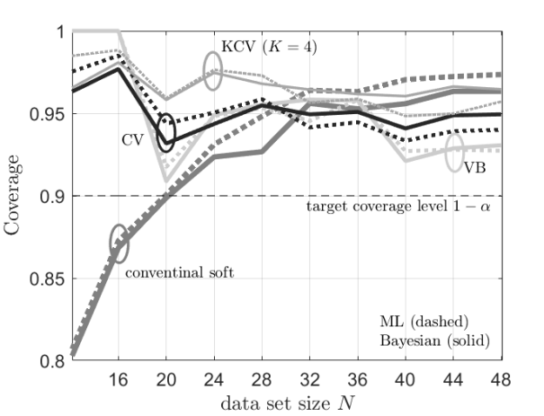
Fig. 2: Coverage for naïve predictor, validation-based (VB) conformal predictor (3.2), cross-validation-based (CV) conformal predictor, (3.3), and the $K$-fold CV ($K$-CV) predictor as a function of the number of pilots $N$. The NC scores are evaluated either using frequentist learning (dashed lines) or Bayesian learning (solid lines).

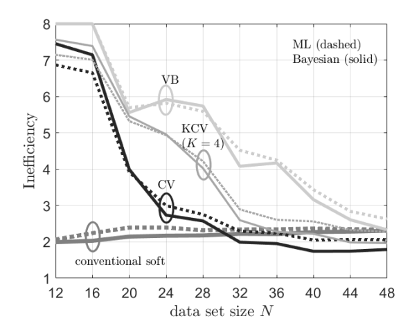
Fig. 3: Average set prediction size (inefficiency) for the same setting of Fig. 2.

Fig. 2 shows the empirical coverage level and Fig. 3 shows the empirical inefficiency, both evaluated on a test set with $100$ samples, as function of the size $N$ of the available data set ${\mathcal{D}}$. We further average the results for 50 independent frames, each corresponding to independent draws of pilot and data symbols from the ground truth distribution. From Fig. 2, we first observe that the naïve set predictor, with both frequentist and Bayesian learning, does not meet the desired coverage level in the regime of a small number $N$ of available samples. In contrast, confirming the theoretical guarantees presented in Sec. 3, all CP methods provide coverage guarantees, achieving coverage rates above $1-\alpha$. From Fig. 3, we observe that the size of the prediction sets, and hence the inefficiency, decreases as the data set size, $N$, increases. Furthermore, due to their efficient use of the available data, CV and $K$-CV predictors have a lower inefficiency as compared to VB predictors. Finally, Bayesian NC scores are generally seen to yield set predictors with lower inefficiency, confirming the merits of Bayesian learning in terms of calibration.

Overall, the experiments confirm that all the CP-based predictors are all well-calibrated with small average set prediction size, unlike naïve set predictors that built directly on the self-reported confidence levels of conventional probabilistic predictors.

References

- [1] Sangwoo Park, Hyeryung Jang, Osvaldo Simeone, and Joonhyuk Kang, “Learning to Demodulate From Few Pilots via Offline and Online Meta-Learning,” IEEE Transactions on Signal Processing, vol. 69, pp. 226–239, 2021.
- [2] Hyeji Kim, Yihan Jiang, Ranvir B Rana, Sreeram Kannan, Sewoong Oh, and Pramod Viswanath, “Communication Algorithms via Deep Learning,” in International Conference on Learning Representations, 2018.
- [3] Yihan Jiang, Hyeji Kim, Himanshu Asnani, and Sreeram Kannan, “Mind: Model Independent Neural Decoder,” in Proc. 2019 IEEE 20th Inter. Workshop on on Signal Processing Advances in Wireless Communications (SPAWC) in Cannes, France. IEEE, 2019, pp. 1–5.
- [4] Chuan Guo, Geoff Pleiss, Yu Sun, and Kilian Q Weinberger, “On Calibration of Modern Neural Networks,” in International Conference on Machine Learning. PMLR, 2017, pp. 1321–1330.
- [5] Andres Masegosa, “Learning under Model Misspecification: Applications to Variational and Ensemble Methods,” Proc. Advances in NIPS, vol. 33, pp. 5479–5491, 2020.
- [6] Warren R Morningstar, Alex Alemi, and Joshua V Dillon, “PACm-Bayes: Narrowing the Empirical Risk Gap in the Misspecified Bayesian Regime,” in Proc. International Conference on Artificial Intelligence and Statistics. PMLR, 2022, pp. 8270–8298.
- [7] Matteo Zecchin, Sangwoo Park, Osvaldo Simeone, Marios Kountouris, and David Gesbert, “Robust PACm: Training Ensemble Models Under Model Misspecification and Outliers,” arXiv preprint arXiv:2203.01859, 2022.
- [8] Patrick Cannon, Daniel Ward, and Sebastian M Schmon, “Investigating the Impact of Model Misspecification in Neural Simulation-based Inference,” arXiv preprint arXiv:2209.01845, 2022.
- [9] David T Frazier, Christian P Robert, and Judith Rousseau, “Model Misspecification in Approximate Bayesian Computation: Consequences and Diagnostics,” Journal of the Royal Statistical Society: Series B (Statistical Methodology), vol. 82, no. 2, pp. 421–444, 2020.
- [10] James Ridgway, “Probably Approximate Bayesian Computation: Nonasymptotic Convergence of ABC under Misspecification,” arXiv preprint arXiv:1707.05987, 2017.
- [11] Vladimir Vovk, Alex Gammerman, and Glenn Shafer, Algorithmic Learning in a Random World, Springer, 2005, Springer, New York.
- [12] Glenn Shafer and Vladimir Vovk, “A Tutorial on Conformal Prediction,” Journal of Machine Learning Research, vol. 9, no. 3, 2008.
- [13] Matteo Fontana, Gianluca Zeni, and Simone Vantini, “Conformal Prediction: a Unified Review of Theory and New Challenges,” arXiv preprint arXiv:2005.07972, 2020.
- [14] Kfir M. Cohen, Sangwoo Park, Osvaldo Simeone, and Shlomo Shamai, “Learning to Learn to Demodulate with Uncertainty Quantification via Bayesian Meta-Learning,” in Proc. WSA 2021; 25th International ITG Workshop on Smart Antennas in EURECOM, France. VDE, 2021, pp. 202–207.
- [15] Zheng Demeng, Yuan Jianguo, Wang Zhe, Zeng Jing, and Sun Lele, “A Two-Stage Coded Modulation Scheme Based on the 8-QAM Signal for Optical Transmission Systems,” Procedia computer science, vol. 131, pp. 964–969, 2018.
- [16] Deepaknath Tandur and Marc Moonen, “Joint Adaptive Compensation of Transmitter and Receiver IQ Imbalance under Carrier Frequency Offset in OFDM-Based Systems,” IEEE Transactions on Signal Processing, vol. 55, no. 11, pp. 5246–5252, 2007.
- [17] Charles Blundell, Julien Cornebise, Koray Kavukcuoglu, and Daan Wierstra, “Weight Uncertainty in Neural Network,” in International Conference on Machine Learning. PMLR, 2015, pp. 1613–1622.
- [18] Osvaldo Simeone, Machine Learning for Engineers, Cambridge University Press, 2022.
- [19] Rina Foygel Barber, Emmanuel J Candes, Aaditya Ramdas, and Ryan J Tibshirani, “Predictive Inference with the Jackknife+,” The Annals of Statistics, vol. 49, no. 1, pp. 486–507, 2021.
- [20] Yaniv Romano, Matteo Sesia, and Emmanuel Candes, “Classification with Valid and Adaptive Coverage,” Advances in NIPS, vol. 33, pp. 3581–3591, 2020.
- [21] Max Welling and Yee W Teh, “Bayesian Learning via Stochastic Gradient Langevin Dynamics,” in Proceedings of the 28th International Conference on Machine learning (ICML-11) in Bellevue, Washington, USA. Citeseer, 2011, pp. 681–688.