FLamby: Datasets and Benchmarks for Cross-Silo Federated Learning in Realistic Healthcare Settings

Abstract

Federated Learning (FL) is a novel approach enabling several clients holding sensitive data to collaboratively train machine learning models, without centralizing data. The cross-silo FL setting corresponds to the case of few ($2$–$50$) reliable clients, each holding medium to large datasets, and is typically found in applications such as healthcare, finance, or industry. While previous works have proposed representative datasets for cross-device FL, few realistic healthcare cross-silo FL datasets exist, thereby slowing algorithmic research in this critical application. In this work, we propose a novel cross-silo dataset suite focused on healthcare, FLamby (Federated Learning AMple Benchmark of Your cross-silo strategies), to bridge the gap between theory and practice of cross-silo FL. FLamby encompasses 7 healthcare datasets with natural splits, covering multiple tasks, modalities, and data volumes, each accompanied with baseline training code. As an illustration, we additionally benchmark standard FL algorithms on all datasets. Our flexible and modular suite allows researchers to easily download datasets, reproduce results and re-use the different components for their research. FLamby is available at www.github.com/owkin/flamby.

1 Introduction

Recently it has become clear that, in many application fields, impressive machine learning (ML) task performance can be reached by scaling the size of both ML models and their training data while keeping existing well-performing architectures mostly unaltered [sun2017revisiting, kaplan2020scaling, chowdhery2022palm, dalle2]. In this context, it is often assumed that massive training datasets can be collected and centralized in a single client in order to maximize performance. However, in many application domains, data collection occurs in distinct sites (further referred to as clients, e.g., mobile devices or hospitals), and the resulting local datasets cannot be shared with a central repository or data center due to privacy or strategic concerns [dwork2014algorithmic, burki2019pharma].

To enable cooperation among clients given such constraints, Federated Learning (FL) [mcmahan2017communication, kairouz2019advances] has emerged as a viable alternative to train models across data providers without sharing sensitive data. While initially developed to enable training across a large number of small clients, such as smartphones or Internet of Things (IoT) devices, it has been then extended to the collaboration of fewer and larger clients, such as banks or hospitals. The two settings are now respectively referred to as cross-device FL and cross-silo FL, each associated with specific use cases and challenges [kairouz2019advances].

On the one hand, cross-device FL leverages edge devices such as mobile phones and wearable technologies to exploit data distributed over billions of data sources [mcmahan2017communication, bonawitz2017practical, bhowmick2018protection, niu2020billion]. Therefore, it often requires solving problems related to edge computing [he2020group, lim2020federated, xia2021survey], participant selection [kairouz2019advances, yang2021achieving, charles2021large, fraboni2021impact], system heterogeneity [kairouz2019advances], and communication constraints such as low network bandwidth and high latency [sattler2019sparse, lu2020low, haddadpour2021federated]. On the other hand, cross-silo initiatives enable to untap the potential of large datasets previously out of reach. This is especially true in healthcare, where the emergence of federated networks of private and public actors [rieke2020future, sheller2020federated, pati2021federated], for the first time, allows scientists to gather enough data to tackle open questions on poorly understood diseases such as triple negative breast cancer [du2021collaborative] or COVID-19 [dayan2021federated]. In cross-silo applications, each silo has large computational power, a relatively high bandwidth, and a stable network connection, allowing it to participate to the whole training phase. However, cross-silo FL is typically characterized by high inter-client dataset heterogeneity and biases of various types across the clients [pati2021federated, du2021collaborative].

As we show in Section 2, publicly available datasets for the cross-silo FL setting are scarce. As a consequence, researchers usually rely on heuristics to artificially generate heterogeneous data partitions from a single dataset and assign them to hypothetical clients. Such heuristics might fall short of replicating the complexity of natural heterogeneity found in real-world datasets. The example of digital histopathology [veta2014breast], a crucial data type in cancer research, illustrates the potential limitations of such synthetic partition methods. In digital histopathology, tissue samples are extracted from patients, stained, and finally digitized. In this process, known factors of data heterogeneity across hospitals include patient demographics, staining techniques, storage methodologies of the physical slides, and digitization processes [janowczyk2019histoqc, fu2020pan, howard2021impact]. Although staining normalization [lahiani2020seamless, de2021deep] has seen recent progress, mitigating this source of heterogeneity, the other highlighted sources of heterogeneity are difficult to replicate with synthetic partitioning [howard2021impact] and some may be unknown, which calls for actual cross-silo cohort experiments. This observation is also valid for many other application domains, e.g. radiology [hahn2006adrenal], dermatology [badano2015consistency], retinal images [badano2015consistency] and more generally computer vision [torralba2011unbiased].

In order to address the lack of realistic cross-silo datasets, we propose FLamby, an open source cross-silo federated dataset suite with natural partitions focused on healthcare, accompanied by code examples, and benchmarking guidelines. Our ambition is that FLamby becomes the reference benchmark for cross-silo FL, as LEAF [caldas2018leaf] is for cross-device FL. To the best of our knowledge, apart from some promising isolated works to build realistic cross-silo FL datasets (see Section 2), our work is the first standard benchmark allowing to systematically study healthcare cross-silo FL on different data modalities and tasks.

To summarize, our contributions are threefold:

1. We build an open-source federated cross-silo healthcare dataset suite including $7$ datasets. These datasets cover different tasks (classification / segmentation / survival) in multiple application domains and with different data modalities and scale. Crucially, all datasets are partitioned using natural splits.

2. We provide guidelines to help compare FL strategies in a fair and reproducible manner, and provide illustrative results for this benchmark.

3. We make open-source code accessible for benchmark reproducibility and easy integration in different FL frameworks, but also to allow the research community to contribute to FLamby development, by adding more datasets, benchmarking types and FL strategies.

This paper is organized as follows. Section 2 reviews existing FL datasets and benchmarks, as well as client partition methods used to artificially introduce data heterogeneity. In Section 3, we describe our dataset suite in detail, notably its structure and the intrinsic heterogeneity of each federated dataset. Finally, we define a benchmark of several FL strategies on all datasets and provide results thereof in Section 4.

2 Related Work

In FL, data is collected locally in clients in different conditions and without coordination. As a consequence, clients’ datasets differ both in size (unbalanced) and in distribution (non-IID) [mcmahan2017communication]. The resulting statistical heterogeneity is a fundamental challenge in FL [li2020suvey, kairouz2019advances], and it is necessary to take it into consideration when evaluating FL algorithms. Most FL papers simulate statistical heterogeneity by artificially partitioning classic datasets, e.g., CIFAR-10/100 [Krizhevsky09learningmultiple], MNIST [lecun-mnisthandwrittendigit-2010] or ImageNet [deng2009imagenet], on a given number of clients. Common approaches to produce synthetic partitions of classification datasets include associating samples from a limited number of classes to each client [mcmahan2017communication], Dirichlet sampling on the class labels [hsu2019measuring, yurochkin2019bayesian], and using Pachinko Allocation Method (PAM) [li2006pachinko, reddi2020adaptive] (which is only possible when the labels have a hierarchical structure). In the case of regression tasks, [philippenko2020bidirectional] partitions the superconduct dataset [caruana2004kdd] across 20 clients using Gaussian Mixture clustering based on T-SNE representations [van2008visualizing] of the features. Such synthetic partition approaches may fall short of modelling the complex statistical heterogeneity of real federated datasets. Evaluating FL strategies on datasets with natural client splits is a safer approach to ensuring that new strategies address real-world issues.

Table 1: Overview of the datasets, tasks, metrics and baseline models in FLamby. For Fed-Camelyon16 the two different sizes refer to the size of the dataset before and after tiling.

Dataset	Fed-Camelyon16	Fed-LIDC-IDRI	Fed-IXI	Fed-TCGA-BRCA	Fed-KITS2019	Fed-ISIC2019	Fed-Heart-Disease
Input (x)	Slides	CT-scans	T1WI	Patient info.	CT-scans	Dermoscopy	Patient info.
Preprocessing	Matter extraction + tiling	Patch Sampling	Registration	None	Patch Sampling	Various image transforms	Removing missing data
Task type	binary classification	3D segmentation	3D segmentation	survival	3D segmentation	multi-class classification	binary classification
Prediction (y)	Tumor on slide	Lung Nodule Mask	Brain mask	Risk of death	Kidney and tumor masks	Melanoma class	Heart disease
Center extraction	Hospital	Scanner Manufacturer	Hospital	Group of Hospitals	Group of Hospitals	Hospital	Hospital
Thumbnails
Original paper	Litjens et al. 2018	Armato et al. 2011	Perez et al. 2021	Liu et al. 2018	Heller et al. 2019	Tschandl et al. 2018 / Codella et al. 2017 / Combalia et al. 2019	Janosi et al. 1988
# clients	2	4	3	6	6	6	4
# examples	399	1,018	566	1, 088	96	23, 247	740
# examples per center	239, 150	670, 205, 69, 74	311, 181, 74	311, 196, 206, 162, 162, 51	12, 14, 12, 12,   16, 30	12413, 3954, 3363, 2259, 819, 439	303, 261, 46, 130
Model	DeepMIL [deepmil]	Vnet [milletari2016v, adaloglou2019MRIsegmentation]	3D U-net [cciccek20163d]	Cox Model [cox1972regression]	nnU-Net [isensee2021nnu]	efficientnet [DBLP:journals/corr/abs-1905-11946] + linear layer	Logistic Regression
Metric	AUC	DICE	DICE	C-index	DICE	Balanced Accuracy	Accuracy
Size	50G (850G total)	115G	444M	115K	54G	9G	40K
Image resolution	0.5 µm / pixel	$\sim$1.0 × 1.0 × 1.0 mm / voxel	$\sim$ 1.0 × 1.0 × 1.0 mm / voxel	NA	$\sim$1.0 × 1.0 × 1.0 mm / voxel	$\sim$0.02 mm / pixel	NA
Input dimension	10, 000 x 2048	128 x 128 x 128	48 x 60 x 48	39	64 x 192 x 192	200 x 200 x 3	13

For cross-device FL, the LEAF dataset suite [caldas2018leaf] includes five datasets with natural partition, spanning a wide range of machine learning tasks: natural language modeling (Reddit [volskeetal2017tl]), next character prediction (Shakespeare [mcmahan2017communication]), sentiment analysis (Sent140 [go2009twitter]), image classification (CelebA [liu2015deep]) and handwritten-character recognition (FEMNIST [cohen2017emnist]). TensorFlow Federated [bonawitz2019towards] complements LEAF and provides three additional naturally split federated benchmarks, i.e., StackOverflow [tenso2019stack], Google Landmark v2 [hsu2020federated] and iNaturalist [horn2018inaturalist]. Further, FLSim [flsim] provides cross-device examples based on LEAF and CIFAR10 [Krizhevsky09learningmultiple] with a synthetic split, and FedScale [lai2022fedscale] introduces a large FL benchmark focused on mobile applications. Apart from iNaturalist, the aforementioned datasets target the cross-device setting.

To the best of our knowledge, no extensive benchmark with natural splits is available for cross-silo FL. However, some standalone works built cross-silo datasets with real partitions. [gong2021ensemble] and [marfoq20neurips] partition Cityscapes [Cordts2016Cityscapes] and iNaturalist [horn2018inaturalist], respectively, exploiting the geolocation of the picture acquisition site. [icml2020_3152] releases a real-world, geo-tagged dataset of common mammals on Flickr. [luo2019real] gathers a federated cross-silo benchmark for object detection created using street cameras. [corinzia2019variational] partitions Vehicle Sensor Dataset [duarte2004vehicle] and Human Activity Recognition dataset [anguita2013public] by sensor and by individuals, respectively. [luofediris] builds an iris recognition federated dataset across five clients using multiple iris datasets [wei2007nonlinear, zhang2010contact, zhang2018deep, phillips2008iris]. While FedML [he2020fedml] introduces several cross-silo benchmarks [he2021fedcv, yuchen2022fednlp, he2021fedgraphnn], the related client splits are synthetically obtained with Dirichlet sampling and not based on a natural split. Similarly, FATE [fate] provides several cross-silo examples but, to the best of our knowledge, none of them stems from a natural split.

In the medical domain, several works use natural splits replicating the data collection process in different hospitals: the works [andreux2020siloed, chakravarty2021federated, baheti2020federated, kaissis2021end, xie2022fedmed, chang2018distributed] respectively use the Camelyon datasets [litjens20181399, bejnordi2017diagnostic, bandi2018detection], the CheXpert dataset [irvin2019chexpert], LIDC dataset [armato2011lidc], the chest X-ray dataset [kermany2018identifying], the IXI dataset [xie2022fedmed], the Kaggle diabetic retinopathy detection dataset [graham2015kaggle]. Finally, the works  [andreux2020federated, gunesli2021feddropoutavg, lu2022federated] use the TCGA dataset [tomczak2015cancer] by extracting the Tissue Source site metadata.

Our work aims to give more visibility to such isolated cross-silo initiatives by regrouping seven medical datasets, some of which listed above, in a single benchmark suite. We also provide reproducible code alongside precise benchmarking guidelines in order to connect past and subsequent works for a better monitoring of the progress in cross-silo FL.

3 The FLamby Dataset Suite

3.1 Structure Overview

The FLamby datasets suite is a Python library organized in two main parts: datasets with corresponding baseline models, and FL strategies with associated benchmarking code. The suite is modular, with a standardized simple application programming interface (API) for each component, enabling easy re-use and extensions of different components. Further, the suite is compatible with existing FL software libraries, such as FedML [he2020fedml], Fed-BioMed [silva2020fed], or Substra [galtier2019substra]. Listing 2 provides a code example of how the structure of FLamby allows to test new datasets and strategies in a few lines of code, and Table 1 provides an overview of the FLamby datasets.

Dataset and baseline model.

The FLamby suite contains datasets with a natural notion of client split, as well as a predefined task and associated metric. A train/test set is predefined for each client to enable reproducible comparisons. We further provide a baseline model for each task, with a reference implementation for training on pooled data. For each dataset, the suite provides documentation, metadata and helper functions to: 1. download the original pooled dataset; 2. apply preprocessing if required, making it suitable for ML training; 3. split each original pooled dataset between its natural clients; and 4. easily iterate over the preprocessed dataset. The dataset API relies on PyTorch [paszke2019pytorch], which makes it easy to iterate over the dataset with natural splits as well as to modify these splits if needed.

FL strategies and benchmark.

FL training algorithms, called strategies in the FLamby suite, are provided for simulation purposes. In order to be agnostic to existing FL libraries, these strategies are provided in plain Python code. The API of these strategies is standardized and compatible with the dataset API, making it easy to benchmark each strategy on each dataset. We further provide a script performing such a benchmark for illustration purposes. We stress the fact that it is easy to alternatively use implementations from existing FL libraries.

3.2 Datasets, Metrics and Baseline Models

We provide a brief description of each dataset in the FLamby dataset suite, which is summarized in Table 1. In Section 3.4, we further explore the heterogeneity of each dataset, as displayed in Figure 1.

Fed-Camelyon16.

Camelyon16 [litjens20181399] is a histopathology dataset of 399 digitized breast biopsies’ slides with or without tumor collected from two hospitals: Radboud University Medical Center (RUMC) and University Medical Center Utrecht (UMCU). By recovering the original split information we build a federated version of Camelyon16 with 2 clients. The task consists in binary classification of each slide, which is challenging due to the large size of each image ($10^{5}\times 10^{5}$ pixels at 20X magnification), and measured by the Area Under the ROC curve (AUC).

As a baseline, we follow a weakly-supervised learning approach. Slides are first converted to bags of local features, which are one order of magnitude smaller in terms of memory requirements, and a model is then trained on top of this representation. For each slide, we detect regions with a matter-detection network and then extract features from each tile with an ImageNet-pretrained Resnet50, following state-of-the-art practice [courtiol2018classification, lu2021data]. Note that due to the imbalanced distribution of tissue in the different slides, a different number of features is produced for each slide: we cap the total number of tiles to $10^{5}$ and use zero-padding for consistency. We then train a DeepMIL architecture [ilse2018attention], using its reference implementation [deepmil] and hyperparameters from [dehaene2020self]. We refer to Appendix C for more details.

Fed-LIDC-IDRI.

LIDC-IDRI [armato2011lidc, lidcdata, clark2013cancer] is an image database [clark2013cancer] study with 1018 CT-scans (3D images) from The Cancer Imaging Archive (TCIA), proposed in the LUNA16 competition [setio2017validation]. The task consists in automatically segmenting lung nodules in CT-scans, as measured by the DICE score [dice1945measures]. It is challenging because lung nodules are small, blurry, and hard to detect. By parsing the metadata of the CT-scans from the provided annotations, we recover the manufacturer of each scanning machine used, which we use as a proxy for a client. We therefore build a 4-client federated version of this dataset, split by manufacturer. Figure 1(b) displays the distribution of voxel intensities in each client.

As a baseline model, we use a VNet [milletari2016v] following the implementation from [adaloglou2019MRIsegmentation]. This model is trained by sampling 3D-volumes into 3D patches fitting in GPU memory. Details of the sampling procedure are available in Appendix D.

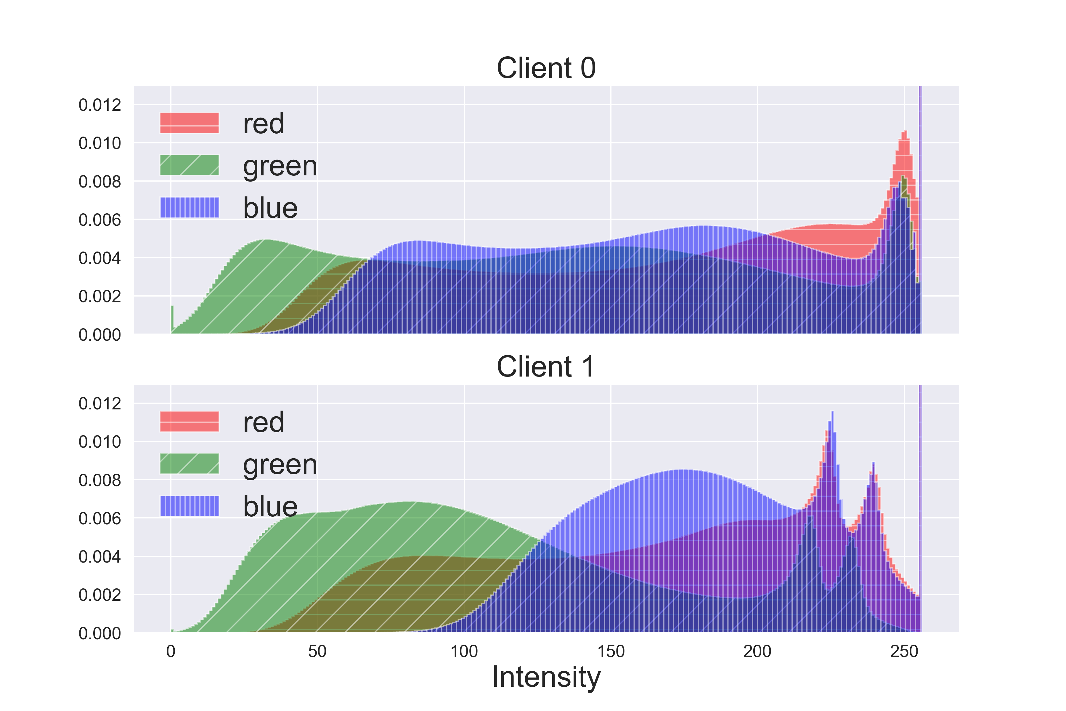
(a) Fed-Camelyon16

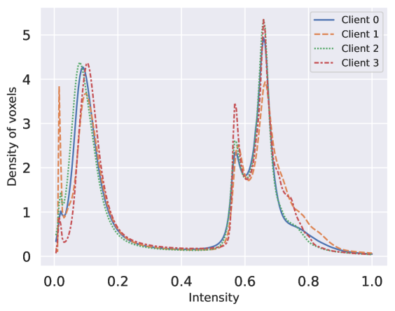
(b) Fed-LIDC-IDRI

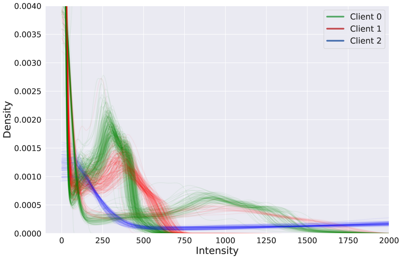
(c) Fed-IXI

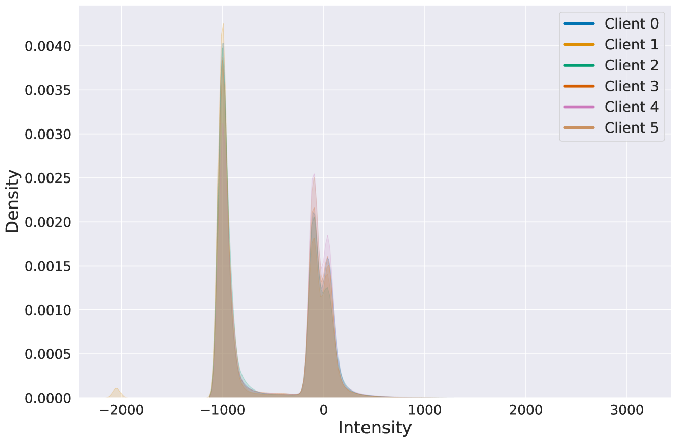
(d) Fed-KITS2019

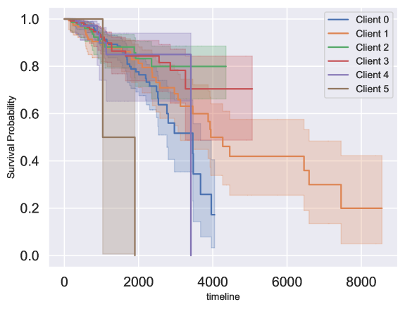
(e) Fed-TCGA-BRCA

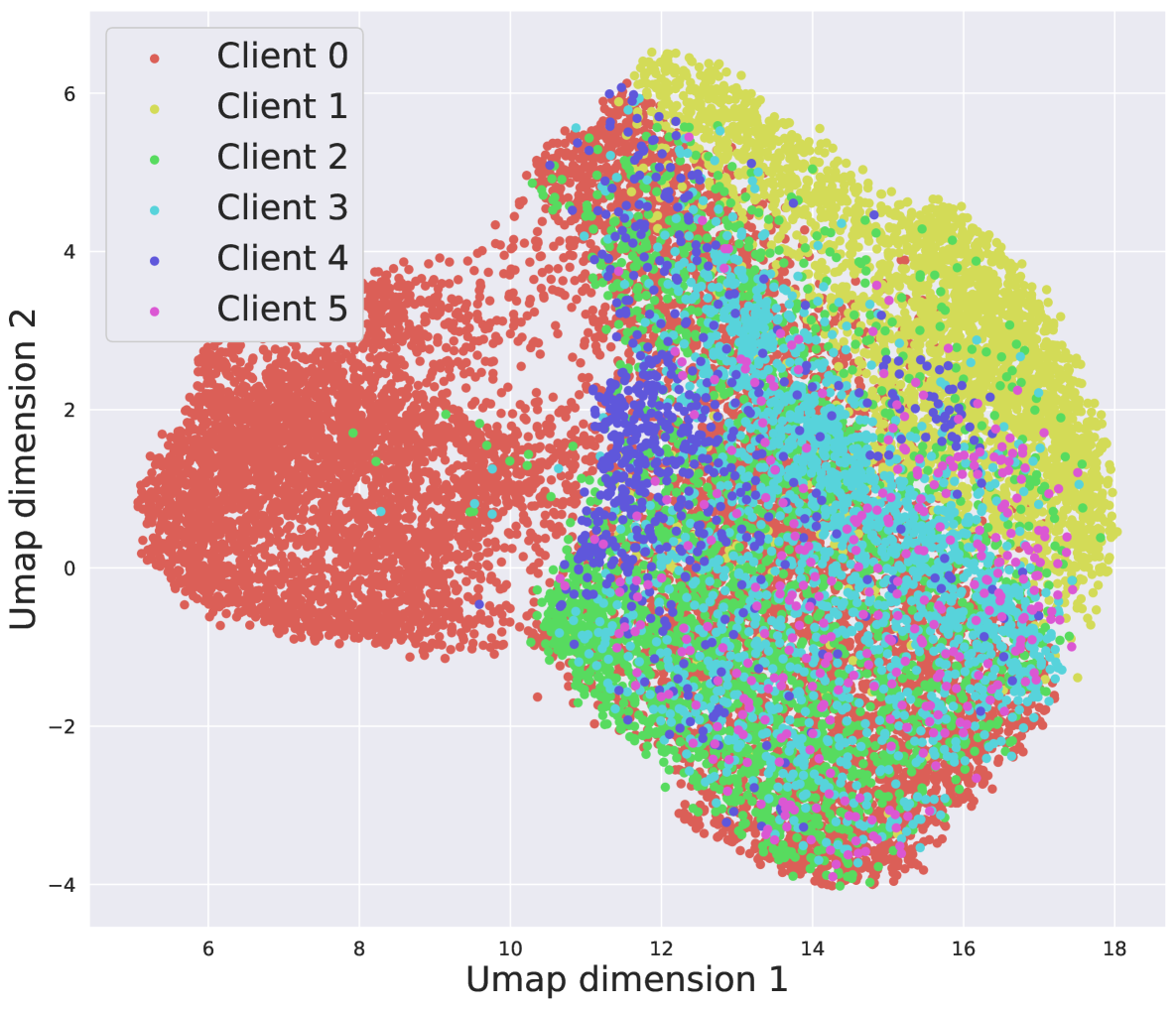
(f) Fed-ISIC2019

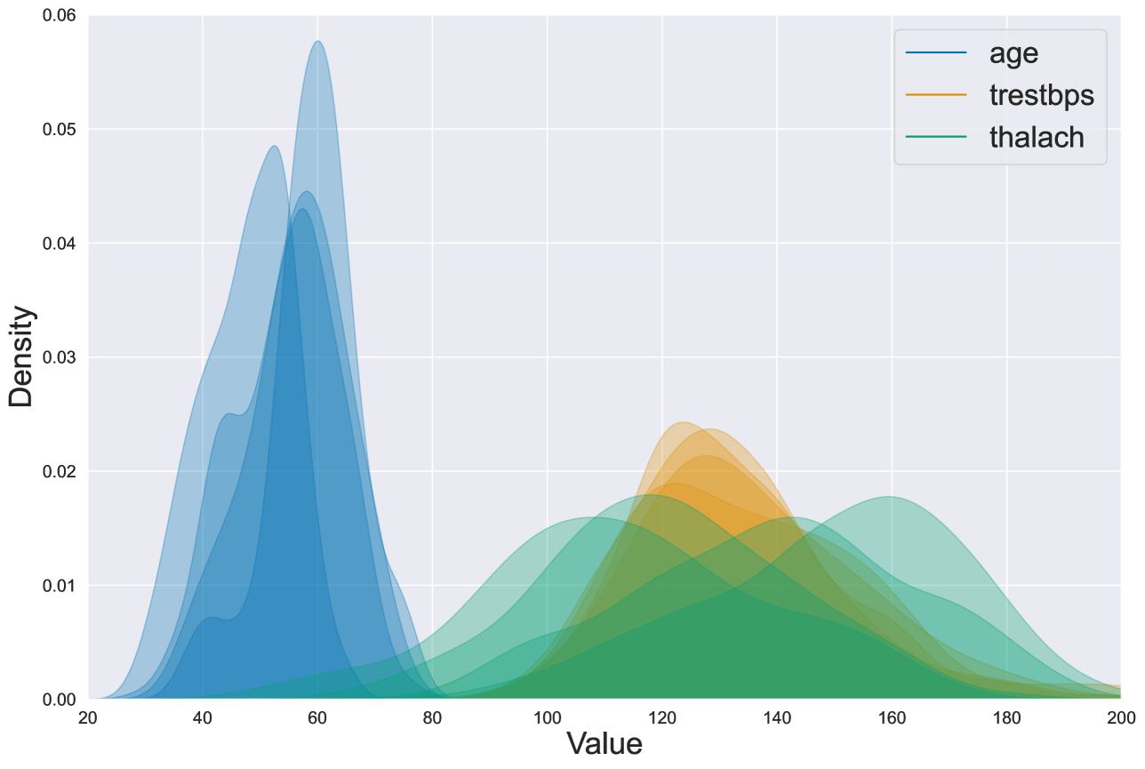
(g) Fed-Heart-Disease

Figure 1: Heterogeneity of FLamby datasets. Best seen in color. 1(a): Color histograms per client. 1(b), 1(c) and 1(d): Voxel intensity distribution per client. 1(e): Kaplan-Meier survival curves per client. 1(f): UMAP of deep network features of the raw images, colored by client. 1(g): Per-client histograms of several features. Differences between client distributions are sometimes obvious and sometimes subtle. Some clients are close in the feature space, some are not and different types of heterogeneity are observed with different data modalities.

Fed-IXI.

This dataset is extracted from the Information eXtraction from Images - IXI database [ixi], and has been previously released by Perez et al. [ixitiny, perez2021torchio] under the name of IXITiny. IXITiny provides a database of brain T1 magnetic resonance images (MRIs) from 3 hospitals (Guys, HH, and IOP). This dataset has been adapted to a brain segmentation task by obtaining spatial brain masks using a state-of-the-art unsupervised brain segmentation tool [iglesias2011robust]. The quality of the resulting supervised segmentation task is measured by the DICE score [dice1945measures].

The image pre-processing pipeline includes volume resizing to $48\times 60\times 48$ voxels, and sample-wise intensity normalization. Figure 1(c) highlights the heterogeneity of the raw MRI intensity distributions between clients. As a baseline, we use a 3D U-net [cciccek20163d] following the implementation of [iximodel]. Appendix E provides more detailed information about this dataset, including demographic information, and about the baseline.

Fed-TCGA-BRCA.

The Cancer Genome Atlas (TCGA)’s Genomics Data Commons (GDC) portal [tcga] contains multi-modal data (tabular, 2D and 3D images) on a variety of cancers collected in many different hospitals. Here, we focus on clinical data from the BReast CAncer study (BRCA), which includes features gathered from 1066 patients. We use the Tissue Source Site metadata to split data based on extraction site, grouped into geographic regions to obtain large enough clients. We end up with 6 clients: USA (Northeast, South, Middlewest, West), Canada and Europe, with patient counts varying from 51 to 311. The task consists in predicting survival outcomes [jenkins2005survival] based on the patients’ tabular data (39 features overall), with the event to predict being death. This survival task is akin to a ranking problem with the score of each sample being known either directly or only by lower bound (right censorship). The ranking is evaluated by using the concordance index (C-index) that measures the percentage of correctly ranked pairs while taking censorship into account.

As a baseline, we use a linear Cox proportional hazard model [cox1972regression] to predict time-to-death for patients. Figure 1(e) highlights the survival distribution heterogeneity between the different clients. Appendix F provides more details on this dataset.

Fed-KITS2019.

The KiTS19 dataset  [heller2020state, heller2019kits19] stems from the Kidney Tumor Segmentation Challenge 2019 and contains CT scans of 210 patients along with the segmentation masks from 79 hospitals. We recover the hospital metadata and extract a 6-client federated version of this dataset by removing hospitals with less than $10$ training samples. The task consists of both kidney and tumor segmentation, labeled 1 and 2, respectively, and we measure the average of Kidney and Tumor DICE scores [dice1945measures] as our evaluation metric.

The preprocessing pipeline comprises intensity clipping followed by intensity normalization, and resampling of all the cases to a common voxel spacing of 2.90x1.45x1.45 mm. As a baseline, we use the nn-Unet library [isensee2021nnu] to train a 3D nnU-Net, combined with multiple data augmentations including scaling, rotations, brightness, contrast, gamma and Gaussian noise with the batch generators framework [isensee2020batchgenerators]. Appendix G provides more details on this dataset.

Fed-ISIC2019.

The ISIC2019 dataset [tschandl2018ham10000, codella2018skin, combalia2019bcn20000] contains dermoscopy images collected in 4 hospitals. We restrict ourselves to 23,247 images from the public train set due to metadata availability reasons, which we re-split into train and test sets. The task consists in image classification among 8 different melanoma classes, with high label imbalance (prevalence ranging 49% to less than 1% depending on the class). We split this dataset based on the imaging acquisition system used: as one hospital used 3 different imaging technologies throughout time, we end up with a 6-client federated version of ISIC2019. We measure classification performance through balanced accuracy, defined as the average recall on each class.

As an offline preprocessing step, we follow recommendations and code from [aman] by resizing images to the same shorter side while maintaining their aspect ratio, and by normalizing images’ brightness and contrast through a color consistency algorithm. As a baseline classification model, we fine-tune an EfficientNet [DBLP:journals/corr/abs-1905-11946] pretrained on ImageNet, with a weighted focal loss [DBLP:journals/corr/abs-1708-02002] and with multiple data augmentations. Figure 1(f) highlights the heterogeneity between the different clients prior to preprocessing. Appendix H provides more details on this dataset.

Fed-Heart-Disease.

The Heart-Disease dataset [janosi1988heart] was collected in 4 hospitals in the USA, Switzerland and Hungary. This dataset contains tabular information about 740 patients distributed among these four clients. The task consists in binary classification to assess the presence or absence of heart disease. We preprocess the dataset by removing missing values and encoding non-binary categorical variables as dummy variables, which gives 13 relevant attributes. As a baseline model, we use logistic regression. Appendix I provides more details on this dataset.

3.3 Federated Learning Strategies in FLamby

The following standard FL algorithms, called strategies, are implemented in FLamby. We rely on a common API for all strategies, which allows for efficient benchmarking of both datasets and strategies, as shown in Listing 2. As we focus on the cross-silo setting, we restrict ourselves to strategies with full client participation.

FedAvg [mcmahan2017communication]. FedAvg is the simplest FL strategy. It performs iterative round-based training, each round consisting in local mini-batch updates on each client followed by parameter averaging on a central server. As a convention, we choose to count the number of local updates in batches and not in local epochs in order to match theoretical formulations of this algorithm; this choice also applies to strategies derived from FedAvg. This strategy is known to be sensitive to heterogeneity when the number of local updates grows [li2020federated, karimireddy2020scaffold].

FedProx [li2020federated]. In order to mitigate statistical heterogeneity, FedProx builds on FedAvg by introducing a regularization term to each local training loss, thereby controlling the deviation of the local models from the last global model.

Scaffold [karimireddy2020scaffold]. Scaffold mitigates client drifts using control-variates and by adding a server-side learning rate. We implement a full-participation version of Scaffold that is optimized to reduce the number of bits communicated between the clients and the server.

Cyclic Learning [chang2018distributed, sheller2018multi]. Cyclic Learning performs local optimizations on each client in a sequential fashion, transferring the trained model to the next client when training finishes. Cyclic is a simple sequential baseline to other federated strategies. For Cyclic, we define a round as a full cycle throughout all clients. We implement both such cycles in a fixed order or in a shuffled order at each round.

FedAdam [reddi2020adaptive], FedYogi [reddi2020adaptive], FedAdagrad [reddi2020adaptive]. FedAdam, FedYogi and FedAdagrad are generalizations of their respective single-centric optimizers (Adam [kingma2014adam], Yogi [zaheer2018adaptive] and Adagrad [lydia2019adagrad]) to the FL setting. In all cases, the running means and variances of the updates are tracked at the server level.

3.4 Dataset Heterogeneity

We qualitatively illustrate the heterogeneity of the datasets of FLamby. For each dataset, we compute a relevant statistical distribution for each client, which differs due to the differences in tasks and modalities of the datasets. We comment the results displayed in Figure 1 in the following. Appendix M provides a more quantitative exploration of this heterogeneity.

For the Fed-Camelyon16 dataset, we display the color histograms (RGB values) of the raw tissue patches in each client. We see that the RGB distributions of both clients strongly differ. For both Fed-LIDC-IDRI and Fed-KITS2019 datasets, we display histograms of voxel intensities. In both cases, we do not note significant differences between clients. For the Fed-IXI dataset, we display the histograms of raw T1-MRI images, showing visible differences between clients. For Fed-TCGA-BRCA, we display Kaplan-Meier estimations of the survival curves [kaplan1958nonparametric] in each client. As detailed in Appendix F, pairwise log-rank tests demonstrate significant differences between some clients, but not all. For the Fed-ISIC2019, we use a 2-dimensional UMAP [mcinnes2018umap] plot of the features extracted from an Imagenet-pretrained Efficientnetv1 on the raw images. We see that some clients are isolated in distinct clusters, while others overlap, highlighting the heterogeneity of this dataset. Last, for the Fed-Heart-Disease dataset, we display histograms for a subset of features (age, resting blood pressure and maximum heart rate), showing that feature distributions vary between clients.

⬇

# Import relevant dataset, strategy, and utilities

from flamby.datasets.fed_camelyon16 import FedCamelyon16, Baseline, BaselineLoss, NUM_CLIENTS, metric

from flamby.strategies import FedProx

from flamby.utils import evaluate_model_on_tests, get_nb_max_rounds

\par# Define number of local updates and number of rounds

num_updates = 100

num_rounds = get_nb_max_rounds(num_updates)

# Dataloaders for train and test

training_dataloaderss = [

DataLoader(FedCamelyon16(center=i, train=True, pooled=False), batch_size=BATCH_SIZE, shuffle=True)

for i in range(NUM_CLIENTS)

]

test_dataloaders = [

DataLoader(FedCamelyon16(center=i, train=False, pooled=False), batch_size=BATCH_SIZE, shuffle=False)

for i in range(NUM_CLIENTS)

]

# Define local model and loss

model_baseline = Baseline()

loss_baseline = BaselineLoss()

# Define and train strategy

strategy = FedProx(training_dataloaders, model_baseline, loss_baseline, torch.optim.SGD, LR, num_updates, num_rounds)

model_final = strategy.run()[0]

# Evaluate final FL model on test sets

results_per_client = evaluate_model_on_tests(model_final, test_dataloaders, metric)

Figure 2: Code example from the FLamby dataset suite: on the Fed-Camelyon16 dataset, we use the FedProx Federated Learning strategy to train the pre-implemented baseline model.

4 FL Benchmark Example with FLamby

In this section, we detail the guidelines we follow to perform a benchmark and provide results thereof. These guidelines might be used in the future to facilitate fair comparisons between potentially novel FL strategies and existing ones. However, we stress that FLamby also allows for any other experimental setup thanks to its modular structure, as we showcase in Appendices L.1 and L.2. The FLamby suite further provides a script to automatically reproduce this benchmark based on configuration files.

Train/test split. We use the per-client train/test splits, including all clients for training. Performance is evaluated on each local test dataset, and then averaged across the clients. We exclude model personalization from this benchmark: therefore, a single model is evaluated at the end of training. We refer to Appendix L.2 for more results with model personalization.

Hyperparameter tuning and Baselines. We distinguish two kinds of hyperparameters: those related to the machine learning (ML) part itself, and those related to the FL strategy. We tune these parameters separately, starting with the machine learning part. All experiments are repeated with 5 independent runs, except for FED-LIDC-IDRI where only 1 training is performed due to a long training time.

For each dataset, the ML hyperparameters include the model architecture, the loss and related hyperparameters, including local batch size. These ML hyperparameters are carefully tuned with cross-validation on the pooled training data. The resulting ML model gives rise to the pooled baseline. We use the same ML hyperparameters for training on each client individually, leading to local baselines.

For the FL strategies, hyperparameters include e.g. local learning rate, server learning rate, and other relevant quantities depending on the strategies. For each dataset and each FL strategy, we use the same model as in the pooled and local baselines, with fixed hyperparameters. We then only optimize FL strategies-related hyperparameters.

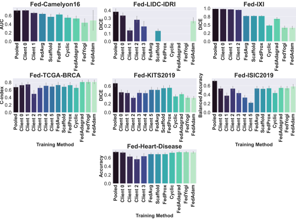
Figure 3: Benchmark results on FLamby for each dataset. For all metrics, higher is better, see Section 3.2 for metric details and Section 4 for experimental details. For Fed-LIDC-IDRI, multiple strategies fail converging, leading to zero DICE. Except for Fed-TCGA-BRCA and Fed-Heart-Disease, federated strategies fall short of reaching the pooled performance, but improve over the local ones.

Federated setup. For all strategies and datasets, the number of rounds $T_{\max}$ is fixed to perform approximately as many epochs on each client as is necessary to get good performance when data is pooled. Note that, as we use a single batch size $B$ and a fixed number $E$ of local steps, the notion of epoch is ill-defined; we approximate it as follows. Given $n_{epochs}^{P}$, the number of epochs required to train the baseline model for the pooled dataset, $n_{T}$ the total number of samples in the distributed training set, $K$ the number of clients, we define

$$T_{\max}=n_{epochs}^{P}\cdot\lfloor n_{T}/K/B/E\rfloor$$ (1)

where $\lfloor\cdot\rfloor$ denotes the floor operation. In our benchmark, we use $E=100$ local updates for all datasets. Note that this restriction in the total number of rounds may have an impact on the convergence of federated strategies. We refer to Appendix J for more details on this benchmark.

Benchmark results. The test results of the benchmark are displayed in Figure 3. Note that test results are uniformly averaged over the different local clients. We observe strikingly different behaviours across datasets.

No local training or FL strategy is able to reach a performance on par with the pooled training, except for Fed-TCGA-BRCA and Fed-Heart-Disease. It is remarkable that both of them are tabular, low-dimensional datasets, with only linear models. Still, for Fed-KITS2019 and Fed-ISIC2019, some FL strategies outperform local training, showing the benefit of collaboration, but falling short of reaching pooled performance. For Fed-Camelyon16, Fed-LIDC-IDRI and Fed-IXI, the current results do not indicate any benefit in collaborative training.

Among FL strategies, we note that for the datasets where an FL strategy outperforms the pooled baselines, FedOpt variants (FedAdagrad, FedYogi and FedAdam) reach the best performance. Further, the Cyclic baseline systematically underperforms other strategies. Last, but not least, FedAvg does not reach top performance among FL strategies, except for Fed-Camelyon16 and Fed-IXI, it remains a competitive baseline strategy.

These results show the difficulty of tuning properly FL strategies, especially in the case of heterogeneous cross-silo datasets. This calls for the development of more robust FL strategies in this setting.

5 Conclusion

In this article we introduce FLamby, a modular dataset suite and benchmark, comprising multiple tasks and data modalities, and reflecting the heterogeneity of real-world healthcare cross-silo FL use cases. This comprehensive benchmark is needed to advance the understanding of cross-silo healthcare data collection on FL performance.

Currently, FLamby is limited to healthcare datasets. In the longer run and with the help of the FL community, it could be enriched with datasets from other application domains to better reflect the diversity of cross-silo FL applications, which is possible thanks to its modular design. Regarding machine learning backends, FLamby only provides PyTorch [paszke2019pytorch] code: supporting other backends, such as TensorFlow [tensorflow2015-whitepaper] or JAX [jax2018github], is a relevant future direction if there is such demand from the community. Further, our benchmark currently does not integrate all constraints of cross-silo FL, especially privacy aspects, which are important in this setting.

In terms of FL setting, the benchmark mainly focuses on the heterogeneity induced by natural splits. In order to make it more realistic, future developments might include in depth study of Differential Privacy (DP) training [dwork2014algorithmic], cryptographic protocols such as Secure Aggregation [bonawitz2017practical], Personalized FL [fallah2020personalized], or communication constraints [sattler2019sparse] when applicable. As we showcase in Appendices L.1 for DP and L.2 for personalization, the structure of FLamby makes it possible to quickly tackle such questions. We hope that the scientific community will use FLamby for cross-silo research purposes on real data, and contribute to further develop it, making it a reference for this research topic.

Checklist

1. For all authors…

   1. Do the main claims made in the abstract and introduction accurately reflect the paper’s contributions and scope? [Yes]

   2. Did you describe the limitations of your work? [Yes] See Section 5.

   3. Did you discuss any potential negative societal impacts of your work? [Yes] See Section A.

   4. Have you read the ethics review guidelines and ensured that your paper conforms to them? [Yes] We point out that we not collect data ourselves. We did a thorough background check on each dataset regarding compliance with these guidelines. We refer to the detailed appendix of each dataset for specific details.

2. If you are including theoretical results…

   1. Did you state the full set of assumptions of all theoretical results? [N/A] Our work does not contain theoretical results.

   2. Did you include complete proofs of all theoretical results? [N/A] Our work does not contain theoretical results.

3. If you ran experiments (e.g. for benchmarks)…

   1. Did you include the code, data, and instructions needed to reproduce the main experimental results (either in the supplemental material or as a URL)? [Yes] See Abstract.

   2. Did you specify all the training details (e.g., data splits, hyperparameters, how they were chosen)? [Yes] See supplementary and code provided.

   3. Did you report error bars (e.g., with respect to the random seed after running experiments multiple times)? [Yes] We reported error bars as we report the average error on the local test sets across multiple seeds. For the largest one, we did not use multiple seeds, but observed empirically a smaller variance in the results due to larger local test set sizes.

   4. Did you include the total amount of compute and the type of resources used (e.g., type of GPUs, internal cluster, or cloud provider)? [Yes] See Appendix J.1

4. If you are using existing assets (e.g., code, data, models) or curating/releasing new assets…

   1. If your work uses existing assets, did you cite the creators? [Yes] See Section 3.

   2. Did you mention the license of the assets? [Yes] See code and supplementary.

   3. Did you include any new assets either in the supplemental material or as a URL? [Yes] See link in abstract.

   4. Did you discuss whether and how consent was obtained from people whose data you’re using/curating? [Yes] We are only repurposing existing assets. We did a thorough background check on each dataset on this issue. We refer to the detailed appendix of each dataset for specific details.

   5. Did you discuss whether the data you are using/curating contains personally identifiable information or offensive content? [Yes] We are only repurposing existing assets. We did a thorough background check on each dataset on this issue. We refer to the detailed appendix of each dataset for specific details.

5. If you used crowdsourcing or conducted research with human subjects…

   1. Did you include the full text of instructions given to participants and screenshots, if applicable? [N/A] We are only repurposing existing assets.

   2. Did you describe any potential participant risks, with links to Institutional Review Board (IRB) approvals, if applicable? [N/A] We are only repurposing existing assets.

   3. Did you include the estimated hourly wage paid to participants and the total amount spent on participant compensation? [N/A] We are only repurposing existing assets.

Appendix A Broader Impact

As this study solely involves the repurposing of existing open-source materials and benchmarking, there are limited risks associated within the study itself. However, it should be noted that all datasets included in this study could be subject to biases originated during the collection process, such as gender or ethnicity biases. Unfortunately, on the images’ datasets (5 datasets out of 7), the sources of such potential biases cannot be easily checked, since data were properly pseudonymised and image-based medical records cannot be straightforwardly tied back to a particular ethnicity or gender by non-medical experts. Nevertheless, as our work exposes more clearly some metadata (e.g. geographical origin) of the datasets, it might help revealing underlying geographical biases, and thus help building more heterogeneous benchmarks, as expected in real scenarios for FL.

As we focused on simplicity and ease of use, the current benchmark does not encompass privacy metrics. However, privacy is of paramount important in healthcare cross-silo FL, and we urge the community not to ignore these aspects. Thanks to the modularity of FLamby, it is easy to add privacy components, as we show in a DP example in Appendix L.1. Thus, we hope FLamby will help tackle privacy questions in healthcare cross-silo FL.

Appendix B Datasets repository and Authors Statement

B.1 Dataset repository.

The code is now available at https://github.com/owkin/FLamby

The code respects best practices for reproducibility and dataset sharing. The installation process is detailed and allow to install only requirements of specific datasets. Regarding code readability, the code is linted with black and flake8 and most functions have docstrings. Documentation is automatically generated from markdown with sphinx, including tutorials. Unit tests ensure FL strategies perform correctly.

Regarding licenses, all datasets documented in this repository come with links towards data terms or licenses. Every time a user downloads a dataset for the first time, he or she is prompted with a link towards the data terms or license, and has to explicitly agree to it in order to proceed.

B.2 Maintenance plan

We will follow a maintenance plan to ensure the code remains correct and the datasets provided by the suite follow adequate standards. In particular, this maintenance plan encompasses:

• Fixing bugs affecting the correctness of the code, whether brought out by the community or ourselves;

• Ensuring security updates in the dependencies are performed;

• Regarding datasets, reviewing, on a monthly basis, potential updates of the datasets referenced in the suite, including but not limited to patients opting out or ethical concerns raised by the work. Such modification may go to the extent of a full revocation of the related dataset if need be;

• Reviewing contributions from the community, whether they are related to the benchmark or to incorporating new datasets to the suite, ensuring they are at the highest standards.

B.3 Authors statement.

As authors of this repository and article we bear all responsibility in case of violation of rights and licenses. We have added a disclaimer on the repository to invite original datasets creators to open issues regarding any license related matters.

Appendix C Fed-Camelyon16

C.1 Description

Camelyon16 litjens20181399 is a histopathology dataset of 399 digitized breast biopsies’ slides with or without tumor collected from two hospitals: Radboud University Medical Center (RUMC) and University Medical Center Utrecht (UMCU). The client information can be read directly from the training slides as the first 170 slides belong to RUMC and the others to UMCU. For the test slides we use a manual approach based on clustering to recover the centres and visual inspection. The slides split are summarized Table 2

Table 2: Information for the different clients in Camelyon16
 

Number	Client	Dataset size	Train	Test
0	RUMC	243	169	74
1	UMCU	156	101	55

C.2 License and Ethics

The Camelyon data is open access (CC0).

The collection of the data was approved by the local ethics committee (Commissie Mensgebonden Onderzoek regio Arnhem - Nijmegen) under 2016-2761, and the need for informed consent was waived litjens20181399.

C.3 Download and preprocessing

As the original dataset is stored in Google Drive, we provide code relying on the Google drive API’s python SDK to batch download all the images (800GB) efficiently. It requires the user to have a Google account and to setup a service account. Detailed instructions are provided in the repository.

Once all tif images have been downloaded we use the histolab packagehistolab to tile the slides with patches of size 224x224 at the second level of the image pyramid corresponding to $\approx 0.5$ µm / pixel. We only keep tiles with sufficient amount of tissue on them thanks to the check_tissue=True} option of the \mintinlinepythonGridTiler histolab object. We then perform Imagenet preprocessing [he2016deep] and extract a 2048 feature vector from an Imagenet-pretrained Resnet50 [he2016deep] on each patch. As slides have different amount of matter this produces a variable number of features per slide. We subsequently save those features in the numpy format [van2011numpy].

C.4 Task

Each of this slide represented as a bag of features has a binary label indicating the presence of a tumour on the breast. The task is to predict if a slide contains a tumour or not so it is framed as a binary classification problem under the Multiple Instance Learning paradigm[deepmil].

C.5 Baseline, loss function and evaluation

Loss function

We use a traditional binary cross entropy loss [good1992rational] and evaluate the performance with the Area under the ROC curve or AUC [bradley1997use].

Baseline Model

We use the DeepMIL[deepmil] architecture that uses attention to learn to weight patch features importance in an end to end fashion. The network architecture is specified in the code. The model trains in approximately 5 minutes on a P100.

Optimization parameters

We use a batch size of 16 with Adam [kingma2014adam] with a learning rate of $0.001$. Both sets of hyperparameters mentioned above used for the network architecture and optimization are taken from [dehaene2020self], we change the number of pooled epochs to 45 in order to be able to do more than one synchronization rounds when performing federated experiments.

Hyperparameter Search

For the pooled dataset benchmark we use the configuration described above without further tuning. For FL strategies we use the following hyperparameter grid: for clients’ learning rates (all strategies) {1e-5, 1e-4, 1e-3, 1e-2, 1e-1, 1.0}; for server size learning rate (for Scaffold and FedOpt strategies) {1e-3, 1e-2, 1e-1, 1.0, 10.0}, and for FedProx only, $\mu$ belongs to {1e-2, 1e-1, 1.0}.

Appendix D Fed-LIDC-IDRI

D.1 Description

LIDC-IDRI [armato2011lidc, lidcdata, clark2013cancer] is part of The Cancer Imaging Archive (TCIA) database [clark2013cancer] with 1009 lung CT-scans (3D images), on which radiologists annotated the presence of nodules.

We split the dataset in 4 different clients that correspond to different medical imagery machine manufacturers, which were previously shown to be a source of heterogeneity in CT image quality [favazza2015cross]. We end up with 661 samples gathered by GE Medical Systems, 205 by Siemens, 69 by Toshiba, and 74 by Philips scanner. These datasets are further split in training and testing sets that contain respectively 80% and 20% of the data. This split is stratified according to clients, so that proportions are respected. The exact distribution of the samples between clients are given in Table 3

Table 3: Information for the different clients in LIDC IDRI.
 

Number	Client	Dataset size	Train	Test
0	GE MEDICAL SYSTEMS	661	530	131
1	Philips	74	59	15
2	SIEMENS	205	164	41
3	TOSHIBA	69	55	14

D.2 License and Ethics

The users of this data must abide by the Data Usage Policies listed on the TCIA webpage under LIDC (links are provided in the README of the LIDC dataset in FLamby repository). It is licensed under a Creative Commons Attribution 3.0 Unported License.

Data was anonymized in each local center before being uploaded to the central repository [armato2011lidc]. Further, as per the terms of use of TCIA, “users must agree not to generate and use information in a manner that could allow the identities of research participants to be readily ascertained”.

D.3 Download and preprocessing

Instructions in the README.md of the LIDC-IDRI dataset in FLamby repository allow to download images and average annotation masks from the TCIA initiative. Flamby code then permits conversion from DICOMs to nifti files to facilitate further analysis.

D.3.1 Preprocessing and sampling

Raw CT scans have varying dimensions which must be standardized prior to training. Therefore, as a first step we resize them to a common $(384,384,384)$ shape by cropping dimensions in excess and reflection-padding missing dimensions. During training, this operation is performed in the same way both on the CT scans and the ground truth masks.

Next, the images are normalized. CT scan voxels are originally expressed in the Hounsfield unit (HU) [feeman2010mathematics] scale: roughly $-1,000$ HU for air, $0$ HU for water, and $1,000$ HU for bone. We clip the images to the $[-1024,600]$ range, add $1024$, and then divide voxels by $1624$ to obtain values ranging in $[0,1]$.

D.4 Task

We benchmark federated learning strategies on a nodule segmentation task using a VNet [milletari2016v]. More precisely, we aim to maximize the DICE coefficient [dice1945measures] between predictions and the annotated ground truths. For reference, the baseline model trained on the pooled training set achieves a DICE of $41\%$ on the pooled test set.

D.5 Baseline, loss function and evaluation

Sampling

The resulting images of size $(384,384,384)$ are too voluminous to fit in the memory of most GPUs. Hence, during training we feed the model with sampled patches of size $(128,128,128)$. We sample $2$ patches from each (image, mask) pair. This implies that batches are constituted of two $(128,128,128)$ patches drawn from the same CT scan. As lung nodules are relatively small and rare, there is a strong class imbalance in the LIDC dataset. To alleviate this issue, we ensure that one of the sampled patches contains nodule voxels (by centering it on a nodule voxel drawn at random), and sample the other completely at random. To account for possible nodules at the edges of CT scans, a padding of half the patch size is applied to each dimension of the image prior to sampling.

Loss function

Our objective is to maximize the DICE coefficient [dice1945measures]. However, we observed that maximizing DICE alone during training yielded poor results at inference time on regions that do not contain nodules. To force the model to account for class imbalance, we added a small balanced cross-entropy term [see jadon2020survey]. Hence, we minimize the following loss:

$$\mathcal{L}(\mathbf{y},\hat{\mathbf{y}})=(1-\mathrm{DICE}(\mathbf{y},\hat{\mathbf{y}}))+0.1\times\mathrm{BCE}(\mathbf{y},\hat{\mathbf{y}}),$$ (2)

with

$$\mathrm{DICE}(\mathbf{y},\hat{\mathbf{y}})=\frac{2\sum_{i=1}^{n}y_{i}\hat{y}_{i}}{\sum_{i=1}^{n}y_{i}+\sum_{i=1}^{n}\hat{y}_{i}},$$ (3)

and

$$\mathrm{BCE}(\mathbf{y},\hat{\mathbf{y}})=-\alpha\sum_{i=1}^{n}y_{i}\log(\hat{y}_{i})-\sum_{i=1}^{n}(1-y_{i})\log(1-\hat{y}_{i}),$$ (4)

where $\alpha=\left(\max(\frac{1}{n}\sum_{i=1}^{n}y_{i},10^{-7})\right)^{-1}-1.$

Baseline Model

We implement a VNet [milletari2016v], following the architecture proposed therein. During training, we use dropout ($p=0.25$). The final layer produces a single output, which is passed through a sigmoid function to encode the probability that each voxel corresponds to a nodule. The model trains in approximately 48 hours on a P100.

Optimization parameters

We optimize the VNet using RMSprop, with an initial learning rate of $10^{-2}$. We run $100$ epochs, multiplying the learning rate by $0.95$ every $10$ epochs.

Hyperparameters search

LIDC FL trainings take approximately 70 hours on a P100 so because of time constraints we could not use an extensive grid search as for other datasets. The final parameters we use are reported in Section J.3.

Appendix E Fed-IXI

E.1 Description

IXI Tiny [ixitiny] is a light version of the dataset IXI, a multimodal brain imaging dataset of almost 600 subjects [ixi]. This lighter version provides T1-weighted brain MR images for a subset of 566 subjects, along with a set of corresponding brain image segmentations labels, taking the form of binary image masks.

Brain image masks isolate the brain pixels from the other head components, such as the eyes, skin, and fat. For the supervised task, brain image segmentation masks (labels) were obtained through automatic whole-brain extraction on the T1-weighted MRI data, using the unsupervised brain extraction tool ROBEX [iglesias2011robust].

The images come from three different London hospitals: Guys (Guy’s Hospital, manufacturer code 0), HH (Hammersmith Hospital, manufacturer code 1), both using a Philips 1.5T system, and IOP (Institute of Psychiatry, manufacturer code 2), using a GE 1.5T system. We split this dataset in training and testing sets, respectively containing 80% and 20% of the data. The split is also stratified according to hospitals to preserve data proportions. In other words, we define one test set on each hospital. Table 4 provides demographic information for this dataset.

Table 4: Demographics information for Fed-IXI.
 

Hospital Name
	Sex	Dataset size	Age	Age Range
Guys	Female	184	53.23 $\pm$ 15.25	20 - 80
	Male	144	51.02 $\pm$ 17.26	20 - 86
HH	Female	93	50.28 $\pm$ 16.93	20 - 81
	Male	85	44.43 $\pm$ 15.67	20 - 73
IOP	Female	44	43.90 $\pm$ 18.43	19 - 86
	Male	24	39.57 $\pm$ 12.46	23 - 70

E.2 License and Ethics

This dataset is licensed under a Creative Commons Attribution Share Alike 3.0 Unported (CC BY-SA 3.) license.

The dataset website does not provide any information regarding data collection ethics. However, the original dataset was collected as part of the IXI - Information eXtraction from Images (EPSRC GR/S21533/02) project, and thus funded by UK Research and Innovation (UKRI). As part of its terms and conditions, the UKRI demands that all funded projects are “carried out in accordance with all applicable ethical, legal and regulatory requirements” (RGC 2.2).

E.3 Downloading and preprocessing

We provide a helper script to download the dataset from an Amazon S3 bucket.

Preprocessing and sampling

We use a fixed preprocessing step that is performed once. Brain scans are first geometrically aligned to a common anatomical space (MNI template) through affine registration estimated with NiftyReg [niftyreg]. Images are then reoriented using ITK [itk]. Finally, intensities are normalized in each image (based on the entire image histogram), and the image volumes are resized from 83x44x55 to 48×60×48 voxels.

E.4 Task

The task is to segment the brain on the volume. The prediction is evaluated with the DICE score, which is the symmetric of the DICE loss with respect to $1/2$.

E.5 Baseline, loss function and evaluation

Loss function

The model was directly trained for the DICE loss [dice1945measures], defined as

$$\ell_{DICE}=1-S_{DICE}=1-\frac{2\mathrm{TP}}{2\mathrm{TP}+\mathrm{FP}+\mathrm{FN}+\epsilon},$$

where $\mathrm{TP}$, $\mathrm{FP}$, and $\mathrm{FN}$ stand for the true positive rate, false positive rate, and false negative rate, respectively, and $\epsilon=10^{-9}$ ensures numerical stability.

Baseline Model

We use a UNet model taking the individual T1 image as input, to predict the associated binary brain mask. The UNet model is a standard type of convolution neural network architecture commonly used in biomedical image segmentation tasks [ronneberger2015u]. It is specifically used to perform semantic segmentation, meaning that each voxel of the image volume is classified. We can also refer to this task as a dense prediction. The model trains in approximately 5 minutes on a P100.

Optimization parameters

The UNet is optimized with a batch size of $2$ and a learning rate of $10^{-3}$ with the AdamW optimizer. The best architecture used batch normalization, max-pooling, linear upsampling, zero-padding of size 1, PReLU activation functions, and 3 encoding blocks.

Hyperparameters search

We do not change parameters for the pooled baseline. For FedAvg and Cyclic, we optimized the learning rate over the values {0.1, 0.01, 0.001, 0.0001, 0.00001}. For FedYogi, FedAdam, FedAdagrad and Scaffold, our search grid space was {0.1, 0.01, 0.001, 0.0001, 0.00001} and {10, 1, 0.1, 0.01, 0.001} for the learning rate and the server learning rate respectively. For FedProx, our search space contained {0.1, 0.01} and {1, 0.1, 0.01} sets for learning rate and $\mu$ respectively.

Appendix F Fed-TCGA-BRCA

F.1 Description

Our dataset comes from The Cancer Genome Atlas (TCGA)’s Genomics Data Commons (GDC) portal [tcga] more specifically from the BReast CAncer study (BRCA), which includes features gathered from 1066 patients. We use the material produced by Liu et al. [liu2018integrated] as a base file that we further preprocess with one-hot encoding following [andreux2020federated]. This produces a lightweight tabular dataset with 39 input features. Patients’ labels are overall survival time and event status with the event being death. We use the Tissue Source Site metadata to split data based on extraction site, grouped into geographic regions to obtain large enough clients. We end up with 6 clients: USA (Northeast, South, Middlewest, West), Canada and Europe, with patient counts varying from 51 to 311. Our train-test split of the data is stratified per client and event. Table 5 provides details per client for this dataset. Table 6 provides results of pair-wise log-rank tests between the different clients.

F.2 License and Ethics

The data terms can be found on the GDC website. In particular, these terms bind users as to “not attempt to identify individual human research participants from whom the data were obtained”.

As per the TCGA policies, special care was devoted to ensure privacy protection of research subjects, including but not limited to HIPAA compliance. Note that we do not use the genetic part of TCGA whose access is restricted due to its sensitivity.

F.3 Downloading and preprocessing

The pooled TCGA-BRCA dataset requires no downloading or extra-preprocessing as the preprocessed data is now a part of the Flamby repository.

Table 5: Information for the different clients (geographical regions) in Fed-TCGA-BRCA.
 

Number	Client	Dataset size	Train	Test	Censorship ratio
0	USA Northeast	311	248	63	81
1	USA South	196	156	40	80
2	USA West	206	164	42	89
3	USA Midwest	162	129	33	88
4	Europe	162	129	33	94
5	Canada	51	40	11	94

Table 6: Pairwise log-rank $p$-values on the Fed-TCGA-BRCA clients. Some clients have significant differences for a 10% significance threshold.

	Client 1	Client 2	Client 3	Client 4	Client 5
Compared with
Client 0	0.289682	0.066374	0.039892	0.576926	0.200366
Client 1		0.192075	0.161797	0.92917	0.541251
Client 2			0.954475	0.720912	0.256973
Client 3				0.576374	0.127662
Client 4					0.441106

F.4 Task

The task consists in predicting survival outcomes [jenkins2005survival] based on the patients’ clinical tabular data (39 features overall). This survival task is akin to a ranking problem with the score of each sample being known either directly or only by lower bound. Indeed, some patients leave the study before the event of interest is observed, and are labelled as right-censored. Survival analysis aims at solving this type of ranking problem while leveraging right-censored data. The censoring ratio in the TCGA-BRCA study is $86\%$.

The ranking is evaluated by using the concordance index (C-index) that measures the percentage of correctly ranked pairs while taking censorship into account:

$$\mathrm{C-index}=\mathbb{E}_{\begin{subarray}{c}i:\delta_{i}=1\\ j:t_{j}>t_{i}\end{subarray}}\big{[}\mathbbm{1}_{[\eta_{j}<\eta_{i}]}\big{]}$$ (5)

where $\eta_{i}$ is a risk score assigned by our model to a patient $i$. In our case of linear Cox proportional hazard models we use $\eta_{i}=\beta^{T}x_{i}$, where $x_{i}$ are the features for patient $i$ and $\beta$ the learned weights, see Section F.5.

Optimization parameters

For the pooled dataset benchmark, we use the Adam optimizer  [kingma2014adam], with a learning rate of $0.1$ and a batch size of $8$ for $30$ epochs.

F.5 Baseline, loss function and evaluation

Survival analysis background

Let $T$ be the random time-to-death taken from the patient’s population under study. The survival function $S$ is defined as:

$$S(t)=Pr[T>t]$$ (6)

A patient is characterized by its vector of covariates $x$ (clinical data in our case), an observed time point $t$ and an indicator $\delta\in\{0,1\}$ where $\delta=0$ if the event has been censored. A key quantity characterizing the distribution of $S$ is the hazard function $h$. It is the instantaneous rate of occurrence of the event given that it has not yet happened for a patient:

$$h(t,x)=\lim_{dt\to 0}\frac{Pr[t<T<t+dt|x,T>t]}{dt}$$ (7)

Loss function

The simplest model in survival analysis is the linear Cox proportional hazard [cox1972regression]. This model assumes:

$$h(t,x)=h_{0}(t)\exp(\beta^{T}x)$$ (8)

where $h_{0}$ is the baseline hazard function (common to all patients and dependent on time only) and $\beta$ is the vector of parameters of our linear model. $\beta$ is estimated by minimization of the negative Cox partial log-likelihood, which compares relative risk ratios:

$$L(\beta)=-\sum_{i:\delta_{i}=1}\Big{[}\beta^{T}x_{i}-\log\big{(}\sum_{j:t_{j}\geq t_{i}}\exp(\beta^{T}x_{j})\big{)}\Big{]}$$ (9)

where $i$ and $j$ index patients.

We minimize the negative Cox partial log-likelihood by gradient descent w.r.t. $\beta$.

As explained in [andreux2020federated] the Cox partial log-likelihood is not separable with respect to the samples: this means it cannot be expressed as a sum of terms each dependent on a single sample. Hence it is not separable with respect to the clients either. In this work, for simplicity, we decide to ignore this fact in the baseline: we treat each client’s negative Cox partial log-likelihood independently of the others and apply any federated learning strategy logic to the resulting local gradients. Please refer to [andreux2020federated] for a more rigorous treatment of the federated survival analysis problem.

Baseline Model

As a baseline, we use the aforementioned linear Cox proportional hazard model [cox1972regression]. The model trains in a matter of seconds on modern CPUs.

Hyperparameter Search

All the federated learning strategies are tested with the SGD optimizer. We performed a grid search for the federated learning strategies hyperparameters . For FedAvg and Cyclic, we optimized the learning rate over the values {0.1, 0.01, 0.001, 0.0001, 0.00001}. For FedYogi, FedAdam, FedAdagrad and Scaffold, our search grid space was {0.1, 0.01, 0.001, 0.0001, 0.00001} and {10, 1, 0.1, 0.01, 0.001} for the learning rate and the server learning rate respectively. For FedProx, our search space contained {0.1, 0.01} and {1, 0.1, 0.01} sets for learning rate and $\mu$ respectively. The chosen hyperparameters from the HP search can be found in Section J.3.

Appendix G Fed-KiTS19

G.1 Description

The KiTS19 dataset  [heller2020state, heller2019kits19] stems from the Kidney Tumor Segmentation Challenge 2019 and contains CT scans of 210 patients along with the segmentation masks from 77 hospitals. We only consider the training dataset of this challenge as the segmentation masks are not provided for the test dataset. We recover the hospital metadata and extract a 6-client federated version of this dataset by removing hospitals with less than $10$ training samples. Figures 4(a) and  4(b) show the repartition of patients per client before and after this client selection respectively. Table 7 provides further details of the train and test split at each selected client.

G.2 License and Ethics

This dataset is licensed under a Attribution-NonCommercial-ShareAlike 4.0 International (CC-BY-NC-SA) license.

The dataset collection was approved by the Institutional Review Board at the University of Minnesota as Study 1611M00821 [heller2019kits19].

G.3 Downloading and Preprocessing

We use the official KiTS19 repository to download the KiTS19 data. Next, we preprocess this dataset. The first step of the preprocessing is to clip the intensity. We clip the values of each image to the [5th percentile, 95th percentile] range, where 5th percentile and 95th percentile are calculated on the image intensities of each patient’s case separately. After this step, we apply z-scale normalization, where we subtract the mean and divide by the standard deviation of the image intensities. Since KiTS19 dataset comes with inhomogeneous voxel spacing even for the patients data from the same silos, we resample the voxel spacings to the target spacing of 2.90x1.45x1.45 mm for all the samples.

G.4 Task

The task consists of both kidney and tumor segmentation, labeled 1 and 2, respectively. The background is labeled as 0. The score we consider on this dataset is the average of Kidney and Tumor DICE scores [dice1945measures].

G.5 Baseline, loss function and evaluation

Sampling

The image size distribution of the samples of the KiTS19 dataset is heterogeneous. After the resampling detailed in section G.3, the median patient’s data size is [116, 282, 282]. To make our model’s computation memory efficient, we extract a patch of size [64, 192, 192] from each sample during the model training. The number of voxels belonging to the foreground classes (i.e. either Kidney or Tumor) is small compare to the number of voxels belonging to the background class. Therefore, we oversample the foreground classes when taking patches of the samples. More precisely, we use batches of size 2. Each batch contains one patch with the foreground oversampled. Furthermore, we split each silo’s data into training and validation data with 80% and 20% split, respectively. All this pre-processing and patching is done using the nnU-Net library [isensee2021nnu].

(a) Original KiTS19

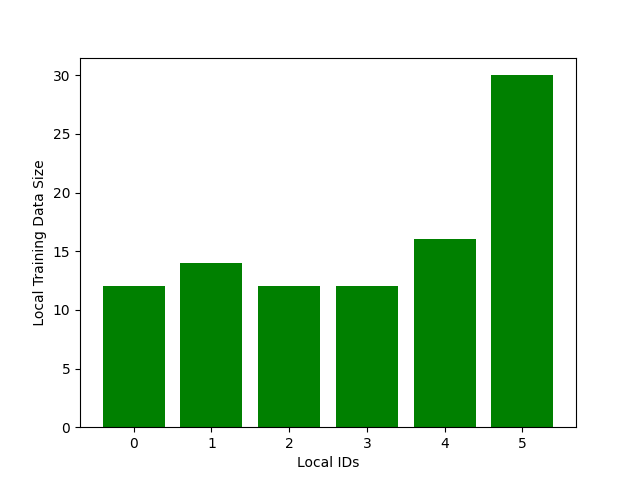
(b) Fed-KiTS19

Figure 4: Patient distributions across hospitals of the original KiTS19 Dataset and the derived Data distribution of Fed-KiTS19

Table 7: Information for the selected clients in Fed-KiTS19.
 

Local ID Number	Dataset size	Train	Test
0	12	9	3
1	14	11	3
2	12	9	3
3	12	9	3
4	16	12	4
5	30	24	6

Loss function

We use the same loss function as proposed by nnU-Net  [isensee2021nnu] for the KiTS19 dataset which is based on DICE [dice1945measures] and on the Cross Entropy loss. Both losses are summed with equal weight as shown in Equation (10),

$$\mathcal{L}(\mathbf{y},\hat{\mathbf{y}})=\mathrm{CE}(\mathbf{y},\hat{\mathbf{y}})-\mathrm{DICE}(\mathbf{y},\hat{\mathbf{y}}),$$ (10)

with

$$\mathrm{DICE}(\mathbf{y},\hat{\mathbf{y}})=\frac{2\sum_{l=1}^{2}\sum_{i=1}^{n}y^{l}_{i}\hat{y}^{l}_{i}+\epsilon}{\sum_{l=1}^{2}(\sum_{i=1}^{n}y^{l}_{i}+\sum_{i=1}^{n}\hat{y}^{l}_{i})+\epsilon},$$ (11)

and

$$\mathrm{CE}(\mathbf{y},\hat{\mathbf{y}})=-\sum_{i=1}^{n}\sum_{l=1}^{2}y^{l}_{i}\log\hat{y}^{l}_{i},$$ (12)

where $\epsilon$ value is $1e^{-5}$ and n is the set of all pixels and 2 signifies the 2 class labels here, Kidney and Tumor, and where $y^{l}_{i}$ is the one-hot encoding (0 or 1) for the label l and pixel $i$ and $y^{l}_{i}$ is the predicted probability for the same label l and pixel $i$.

Baseline Model

During the training, we use nnU-Net [isensee2021nnu], with the architecture proposed therein for the KiTS19 dataset. We chose convolution kernels of sizes [[3,3,3],[3,3,3],[3,3,3],[3,3,3],[3,3,3]] and pool kernels of sizes [[2,2,2],[2,2,2],[2,2,2],[2,2,2],[1,2,2]]. The model trains in under 24 hours on a P100.

Optimization parameters

In addition, we use Adam optimizer  [kingma2014adam] with a learning rate of 0.0003 for 500 epochs to train our model. To evaluate the performance of the trained model, we evaluate the DICE score on the validation data for both classes, Kidney and tumor, and report the average of these two scores. We note that with 8000 epochs we can obtain higher performances, however at the expense of computational cost.

Hyperparameter Search

For the pooled strategy results, we use the Adam Optimizer and 0.0003 learning rate, as used in nnU-Net work for KiTS19 dataset [isensee2021nnu]. For Cyclic and FedAvg, we optimized the learning rate over the values {0.3, 0.03, 0.003, 0.0003, 0.00003} and found that a learning rate of 0.3 provided the best results for both strategies. For FedYogi, FedAdam, FedAdagrad and Scaffold, our search grid space was {0.1, 0.01} and {0.001, 0.01, 0.1, 1} for the learning rate and the server learning rate respectively. In the best setting, the learning rate was $0.1$ for all these strategies, and the server learning rate $0.1$ for FedAdagrad, $0.01$ for FedYogi and FedAdam and $1$ for Scaffold. Likewise, for FedProx, our search space contained {0.1, 0.01} and {0.001, 0.01, 0.1, 1} sets for learning rate and $\mu$ respectively, and the best set of hyperparameters was $0.1$ for the learning rage and $0.001$ for $\mu$.

Appendix H Fed-ISIC2019

H.1 Dataset description

The ISIC2019 challenge dataset [tschandl2018ham10000, codella2018skin, combalia2019bcn20000] contains 25,331 dermoscopy images collected in 4 hospitals. To the best of our knowledge, it is the largest public dataset of high-quality images of skin lesions. We restrict ourselves to 23,247 images from the public train set due to metadata availability reasons, which we re-split into train and test sets. The train-test split is static.

We split this dataset into 6 clients corresponding to different sites where images were taken with different imaging technologies. The ViDIR Group, Medical University of Vienna, Austria uses 3 different imaging systems representing evolving clinical practice: a Heine Dermaphot system using an immersion fluid, a DermLite™ FOTO and a MoleMax HD machine which gives rise to 3 clients. On top of this, the skin cancer practice of Cliff Rosendahl in Queensland, Australia, the Hospital Clínic de Barcelona, Spain and the Memorial Sloan Kettering Cancer Center, New York give rise to 3 other different clients making a total of 6 clients. The biggest client counts 12413 images while the smallest counts 439. Table 8 provides details about the size of the different clients.

Table 8: Information for the different clients in Fed-ISIC2019.
 

Number	Client	Dataset size	Train	Test
0	Hospital Clínic de Barcelona	12413	9930	2483
1	ViDIR Group, Medical University of Vienna (MoleMax HD)	3954	3163	791
2	ViDIR Group, Medical University of Vienna (DermLite FOTO)	3363	2691	672
3	The skin cancer practice of Cliff Rosendahl	2259	1807	452
4	Memorial Sloan Kettering Cancer Center	819	655	164
5	ViDIR Group, Medical University of Vienna (Heine Dermaphot)	439	351	88

H.2 License and Ethics

This dataset is licensed under a Attribution-NonCommercial 4.0 International (CC BY-NC 4.0) license.

As per the terms of use of the ISIC archive, one of the requirements for this dataset to have been hosted is that it is properly de-identified in accordance with applicable requirements and legislations.

H.3 Downloading and preprocessing

Instructions for downloading and preprocessing are available in the README of the Fed-ISIC2019 dataset inside the FLamby repository. As an offline preprocessing step, we follow recommendations and code from [aman] by resizing images to the same shorter side of 224 pixels while maintaining their aspect ratio, and by normalizing images’ brightness and contrast through a color consistency algorithm. The total size of the raw inputs is $9$ GB.

H.4 Task

The task consists in image classification among 8 different classes: Melanoma, Melanocytic nevus, Basal cell carcinoma, Actinic keratosis, Benign keratosis, Dermatofibroma, Vascular lesion and Squamous cell carcinoma. Ground truth is established through histopathology, follow-up examination, expert consensus or microscopy. The ISIC2019 dataset has a high label imbalance with prevalence ranging from 49% to less than 1% depending on the class. We follow the ISIC challenge metric: we measure classification performance through balanced accuracy, defined as the average of the recalls calculated for each class. For balanced datasets, it is equal to accuracy. A random classifier would get a balanced accuracy equal to $1/C$ where $C$ is the number of classes. Using balanced accuracy prevents the model from taking advantage of an imbalanced test set.

H.5 Baseline, loss function and evaluation

The choices made are inspired by [aman],  [DBLP:journals/corr/abs-1910-03910], and an analysis of the solutions that scored well at the ISIC challenge over the years.

Loss function

Our pretrained EfficientNet is fine-tuned using a weighted focal loss [DBLP:journals/corr/abs-1708-02002]. It is calculated as follows:

$$FL(p_{t})=-\alpha_{t}(1-p_{t})^{\gamma}\log(p_{t})$$ (13)

where $p_{t}$ is the probability output by our model for the ground-truth class, $\alpha_{t}$ is the weight of the ground-truth class (a weight is attributed to each class before training), $\gamma$ is a hyperparameter (chosen at $2$ in our work). The focal loss is very useful where there is class imbalance. To provide an intuition behind this focal loss, compared to Binary Cross Entropy, it gives the model a bit more freedom to take some risk when making predictions. The weights we use for our weighted focal loss are the inverse of the class proportions calculated over the pooled dataset. We assume these weights are available to all clients.

Baseline Model

As a baseline classification model, we fine-tune an EfficientNet [DBLP:journals/corr/abs-1905-11946]. EfficientNets are the results of a simple uniform scaling of MobileNets and ResNet on all dimensions (depth/width/resolution). They show great accuracy and efficiency and transfer very well to other tasks. Our EfficientNet is pretrained on ImageNet, we use it as a feature extractor ($1280$ features) by replacing the output layer by a linear layer to get an output of dimension $8$. On top of this, we use the data augmentations listed below to regularize our model. The model trains in under an hour on a P100, because we have to recompute EfficientNet features with dynamic data augmentations.

For training:

1. Random Scaling

2. Rotation

3. Random Brightness Contrast

4. Flipping

5. Affine deformation

6. Random crop

7. Coarse Dropout

8. Normalization

At test time:

1. Center cropping

2. Normalization

Optimization parameters

For the pooled dataset benchmark, we use the Adam optimizer  [kingma2014adam] with a learning rate of $5\times 10^{-4}$ and a batch size of $64$ for $20$ epochs.

Hyperparameter Search

All the federated learning strategies are tested with the SGD optimizer. We performed a grid search for the federated learning strategies hyperparameters. For FedAvg and Cyclic, we optimized the learning rate over the values {1e-3, 1e-2.5, 1e-2, 1e-1.5, 1e-1, 1e-0.5}. For FedYogi, FedAdam, FedAdagrad and Scaffold, our search grid space was {1e-3, 1e-2.5, 1e-2, 1e-1.5, 1e-1, 1e-0.5} and {1e-3, 1e-2.5, 1e-2, 1e-1.5, 1e-1, 1e-0.5, 1, 1e-0.5, 10} for the learning rate and the server learning rate respectively. For FedProx, our search space contained {1e-3, 1e-2.5, 1e-2, 1e-1.5, 1e-1, 1e-0.5} and {0.001, 0.01, 0.1, 1.} sets for learning rate and $\mu$ respectively. The chosen hyperparameters from the HP search can be found in Sec. J.3.

Appendix I Fed-Heart-Disease

I.1 Description

The Heart Disease dataset contains records from 920 patients from four hospitals in the USA, Hungary, and Switzerland. There are 13 features before preprocessing: age, sex, chest pain type, resting blood pressure, serum cholesterol, blood sugar, resting electrochardiographic results, maximum heart rate, exercise induced angina, ST depression induced by exercise, slope of the peak ST segment, number of major vessels, and thalassemia background. All features are continuous or binary, except for chest pain type (four categories) and resting electrochardiographic results (three categories). The target is the presence of a heart disease. After preprocessing, we are left with 740 records, each having 13 features. They are split in train and test in a stratified manner. Distribution of the data records among clients is described in Table 9.

Table 9: Distribution of data records among the different clients in Fed-Heart-Disease.
 

Number	Client	Dataset size	Train	Test
0	Cleveland’s Hospital	303	199	104
1	Hungarian Hospital	261	172	89
2	Switzerland Hospital	46	30	16
3	Long Beach Hospital	130	85	45

I.2 License and Ethics

This dataset is licensed under a Creative Commons Attribution 4.0 International (CC BY 4.0) license [janosi1988heart, dua2019Uci].

Regarding privacy, the dataset authors [janosi1988heart] indicated that sensitive entries of the dataset (including names and social security numbers) were removed from the database.

I.3 Downloading and Preprocessing

Instructions for downloading are available in the corresponding README file on FLamby’s repository. Dataset is downloaded from the UCI Machine Learning repository [dua2019Uci].

We preprocess the dataset by removing the three features (slope of the peak ST segment, number of major vessels, and thalassemia background) where too many entries are missing. We then remove records where at least one feature is missing. Finally, the two categorical (and non binary) features (chest pain type and resting electrochardiographic results) are encoded as binary features using dummy variables. We also normalize features per center.

I.4 Task

The task consists in predicting the presence of a heart disease so the task is binary classification.

I.5 Baseline, Loss Function, and Evaluation

Loss function

For a data record $(x_{i},y_{i})$, we compute the predicted label $\hat{y}_{i}=\sigma(\beta^{T}x_{i})$, where $\sigma(z)=1/(1+\exp(-z))$ is the sigmoid function, and $\beta$ the parameters of the model. We then compute the loss over the complete dataset as

$$L(y,\hat{y})=-\frac{1}{n}\sum_{i=1}^{n}y_{i}\log(\hat{y}_{i})+(1-y_{i})\log(1-\hat{y}_{i})\enspace.$$ (14)

Baseline Model

We fit a logistic regression model, as this is both a standard problem in medical research, and the strongest baseline according to [dua2019Uci]. The model trains in a matter of seconds on modern CPUs.

Evaluation

To evaluate the model, we threshold the predicted values $\hat{y}$ at $0.5$, and measure the accuracy of the obtained labels as

$$Acc(\beta,X,y)=\frac{|\{i\in[n]\mid y_{i}=(\hat{y}_{i}>0.5)\}|}{n}\enspace.$$ (15)

Optimization parameters

For the pooled benchmark, we use the Adam optimizer  [kingma2014adam] with a learning rate of $0.001$, batch size of $4$, for $50$ epochs.

Hyperparameter Search

All the federated learning strategies are tested with the SGD optimizer. We performed a grid search for the federated learning strategies hyperparameters . For FedAvg and Cyclic, we optimized the learning rate over the values {0.1, 0.01, 0.001, 0.0001, 0.00001}. For FedYogi, FedAdam, FedAdagrad and Scaffold, our search grid space was {0.1, 0.01, 0.001, 0.0001, 0.00001} and {10, 1, 0.1, 0.01, 0.001} for the learning rate and the server learning rate respectively. For FedProx, our search space contained {0.001, 0.0001} and {1, 0.1, 0.01} sets for learning rate and $\mu$ respectively. The chosen hyperparameters from the HP search can be found in Section J.

Appendix J Experimental details

Table 10: Hyperparameters used for the FedAvg strategy

FedAvg
dataset	learning rate	optimizer
Fed-Camelyon16	0.3162	torch.optim.SGD
Fed-LIDC-IDRI	0.001	torch.optim.SGD
Fed-IXI	0.001	torch.optim.SGD
Fed-TCGA-BRCA	0.1	torch.optim.SGD
Fed-KITS19	0.03	torch.optim.SGD
Fed-ISIC2019	0.01	torch.optim.SGD
Fed-Heart-Disease	0.001	torch.optim.SGD

Table 11: Hyperparameters used for the FedProx strategy

FedProx
dataset	mu	learning rate	optimizer
Fed-Camelyon16	0.316228	0.01	torch.optim.SGD
Fed-LIDC-IDRI	0.01	0.001	torch.optim.SGD
Fed-IXI	0.1	0.001	torch.optim.SGD
Fed-TCGA-BRCA	0.1	0.1	torch.optim.SGD
Fed-KITS19	0.001	0.1	torch.optim.SGD
Fed-ISIC2019	0.001	0.01	torch.optim.SGD
Fed-Heart-Disease	0.001	0.01	torch.optim.SGD

Table 12: Hyperparameters used for the FedAdagrad strategy

FedAdagrad
dataset	learning rate	optimizer	learning rate server	$\beta_{1}$	$\beta_{2}$	$\tau$
Fed-Camelyon16	0.01	torch.optim.SGD	0.003162
Fed-LIDC-IDRI	0.1	torch.optim.SGD	0.1
Fed-IXI	1e-04	torch.optim.SGD	0.1	0.9	0.999	1e-08
Fed-TCGA-BRCA	0.01	torch.optim.SGD	1.0	0.9	0.999	1e-08
Fed-KITS19	0.1	torch.optim.SGD	0.1	0.9	0.999	1e-08
Fed-ISIC2019	0.01	torch.optim.SGD	0.0316
Fed-Heart-Disease	0.003162	torch.optim.SGD	0.003162	0.9	0.999	0.3162

Table 13: Hyperparameters used for the FedAdam strategy

FedAdam
dataset	learning rate	optimizer	learning rate server	$\beta_{1}$	$\beta_{2}$	$\tau$
Fed-Camelyon16	0.001	torch.optim.SGD	3.1622
Fed-LIDC-IDRI	0.3162	torch.optim.SGD	0.01
Fed-IXI	1e-04	torch.optim.SGD	0.1	0.9	0.999	1e-08
Fed-TCGA-BRCA	0.01	torch.optim.SGD	0.1	0.9	0.999	1e-08
Fed-KITS19	0.1	torch.optim.SGD	0.01	0.9	0.999	1e-08
Fed-ISIC2019	0.01	torch.optim.SGD	0.0032
Fed-Heart-Disease	0.01	torch.optim.SGD	0.01	0.9	0.999	1e-08

Table 14: Hyperparameters used for the FedYogi strategy

FedYogi
dataset	learning rate	optimizer	learning rate server	$\beta_{1}$	$\beta_{2}$	$\tau$
Fed-Camelyon16	0.003162	torch.optim.SGD	1.0
Fed-LIDC-IDRI	0.1	torch.optim.SGD	0.001
Fed-IXI	1e-04	torch.optim.SGD	0.1	0.9	0.999	1e-08
Fed-TCGA-BRCA	0.01	torch.optim.SGD	0.1	0.9	0.999	1e-08
Fed-KITS19	0.1	torch.optim.SGD	0.01	0.9	0.999	1e-08
Fed-ISIC2019	0.01	torch.optim.SGD	0.0032
Fed-Heart-Disease	0.0031622	torch.optim.SGD	0.01	0.9	0.999	1e-08

Table 15: Hyperparameters used for the Cyclic strategy

Cyclic
dataset	learning rate	optimizer
Fed-Camelyon16	0.01	torch.optim.SGD
Fed-LIDC-IDRI	0.0316	torch.optim.SGD
Fed-IXI	1e-05	torch.optim.SGD
Fed-TCGA-BRCA	0.01	torch.optim.SGD
Fed-KITS19	0.3	torch.optim.SGD
Fed-ISIC2019	0.0032	torch.optim.SGD
Fed-Heart-Disease	0.01	torch.optim.SGD

Table 16: Hyperparameters used for the Scaffold strategy

Scaffold
dataset	learning rate	optimizer	learning rate server
Fed-Camelyon16	0.1	torch.optim.SGD	3.1622
Fed-LIDC-IDRI	0.0316	torch.optim.SGD	1.0
Fed-IXI	0.001	torch.optim.SGD	1.0
Fed-TCGA-BRCA	0.01	torch.optim.SGD	1.0
Fed-KITS19	0.1	torch.optim.SGD	1.0
Fed-ISIC2019	0.01	torch.optim.SGD	1.0
Fed-Heart-Disease	0.001	torch.optim.SGD	1.0

J.1 Computing resources

Most experiments were performed on virtual machines equipped with NVidia P100 GPUs in Google Cloud to tune local baselines as well as searching hyperparameters. Additional experiments were also performed on small workstations for the smallest datasets. Overall, no more than 4k GPU-hours were used throughout the full project.

J.2 FLamby experimental capabilities

FLamby is designed to be a lightweight and simple codebase, to enable ease of use. All clients run sequentially in the same python environment, without multithreading. Datasets are assigned to clients as different python objects. GPU acceleration is supported thanks to current PyTorch [paszke2019pytorch] backend. In order to perform more realistic experiments, e.g. to investigate communication constraints, we encourage the usage of dedicated FL libraries, which are easy to integrate with FLamby.

J.3 Benchmark hyperparameters

We used the hyperparameters detailed in Tables 10 to 16 to obtain the results of Figure 3. These hyperparameters were found after hyper-optimization on a coarse grid. For all strategies and datasets, we set $E=100$ the number of local updates.

J.4 Run details

Results of Figure 3 were obtained following 5 independent runs with different random seeds, except for the largest one (Fed-LIDC-IDRI), where computational resources prevented training.

Appendix K Synthetic dataset splits

One of FLamby’s strengths is that it provides datasets with natural splits. However, due to its focus on healthcare applications, the number of clients is limited. Thanks to the standardized API of the datasets, it is possible to create new client splits based on the provided codebase.

We provide an example of such a synthetic sampling based on a Dirichlet distribution on the original clients. If $K$ denotes the previous number of clients and $K^{\prime}$ the desired number of clients, for $\alpha\in(0,1)$, we draw a probability distribution $\mathbf{p}_{k}\in\mathbb{R}^{K^{\prime}}$ as

$$\mathbf{p}_{k}\sim\mathrm{Dir}(\alpha),\text{such that}\sum_{k^{\prime}}p_{kk^{\prime}}=1.$$ (16)

Each sample from client $k$ is then attributed to client $k^{\prime}$ with probability $p_{kk^{\prime}}$, both for the train and test sets. The closer to $0$ $\alpha$ gets, the sharper the distribution probability $\mathbf{p}_{k}$ gets. In order to avoid having empty clients with the synthetic split, we recommend setting $\alpha\geq 1/2$, following previous works [yurochkin2019bayesian].

Appendix L Examples of extensions possible in FLamby

In this Appendix, we showcase the extensibility of FLamby by tackling different FL settings.

L.1 Differential Privacy Example

Differential privacy (DP) [dwork2014algorithmic] is an important approach to protect update exchanges between Federated Learning participants against malicious privacy attacks [wei2020framework]. In this section, we use Fed-Heart-Disease to demonstrate the use of FLamby to study $(\epsilon,\delta)$-DP federated learning [dwork2014algorithmic].

Figure 5 displays the average performance of a machine learning model trained in a differentially private fashion with DP-FedAvg as a function of $\epsilon$ and $\delta$. We compare it to a regular training using the same model initialization but without privacy (“Baseline wo DP”), trained with regular FedAvg. We see the performance diminishing when $\epsilon$ tends to $0$, especially for small values of $\delta$ often used in practice, which is a standard phenomenon.

To implement DP in FedAvg, we use on the DP-SGD mechanism and track the monitoring of privacy budget thanks to the moment accountant [abadi2016deep]. We use the Opacus library [yousefpour2021opacus], which is easy to integrate into FLamby thanks to its modular design.

At this time of writing, Opacus does not support all Deep Learning building blocks such as normalization layers. This prevents applying DP mechanisms on some some of FLamby’s baseline models such as the baseline for Fed-ISIC2019 and Fed-IXI.

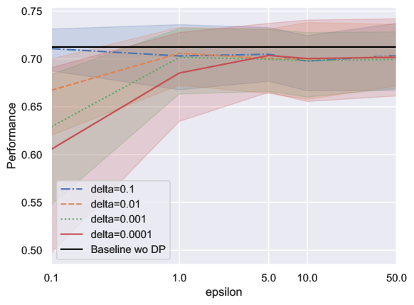
Figure 5: Impact of Differential-Privacy on average performance for DP-FedAvg on Fed-Heart-Disease.

L.2 Personalized Federated Learning

Model personalization [fallah2020personalized] is an effective strategy to improve model performance in cross-silo settings, especially in presence of data heterogeneity. Here, we showcase a simple example of model personalization with FLamby, which is possible thanks to its simple and modular API.

We implement the FedAvg strategy followed by local fine tuning on each center, thus producing as many models as there are clients. We test the addition of such fine-tuning process on the performances of Federated models while testing each model on its corresponding test set. For each dataset, we perform $100$ local updates after the federated averaging training has taken place.

Figure display the training results 6. We see that for Fed-Heart-Disease and Fed-ISIC2019, personalization improves results, while performance is slightly degraded for Fed-Camelyon16. We hope that researchers will be able to investigate more personalization strategies easily with FLamby.

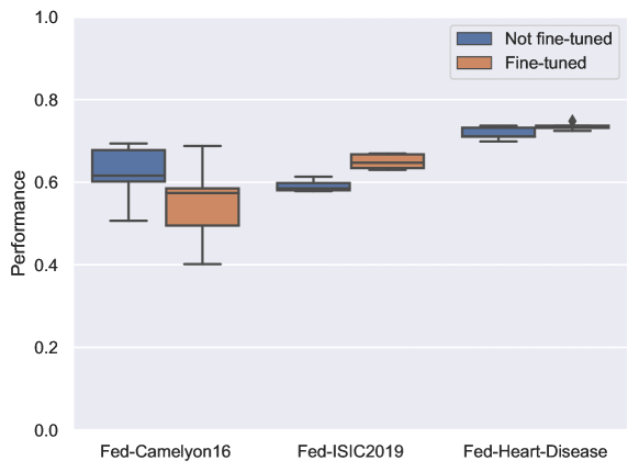
Figure 6: Impact of personalization on test average performance on three datasets of the suite (Fed-Heart-Disease, Fed-Camelyon16 and Fed-ISIC2019) after performing Federated Averaging. In the two extreme cases (Left and Right) fine-tuning is beneficial, whereas on Fed-Camelyon16, Fine-tuning degrades the performance of the resulting models. We hypothesize that, in this case, fine-tuning overfits the local training datasets.

Appendix M Quantitative heterogeneity benchmarks

We describe in this section our analysis of the heterogeneity of the Flamby datasets. Due to the variety of tasks and data, we restrict this study to generic metrics. We always compute them on the whole dataset, putting together test and train data to have the best possible estimation of the underlying distribution.

In the first subsection, we briefly describe the three sources of heterogeneity that we consider. Next, we detail the methodology used to compute statistical distance between clients. Thirdly, we apply this methodology to the FLamby’s dataset. And finally, we provide some discussion on these results.

M.1 Description of measured heterogeneity

Imbalance.

The easiest quantification of heterogeneity comes from the number of samples hosted by each client, which gives natural unbalance in the training because small clients are likely to be either over-fitted or neglected in the final model.

Labels distribution.

Labels can be another source of heterogeneity in case when prediction outputs vary between clients for the considered task. For instance, if a client is specialized in treating the patients with the given disease, the labels are likely to be biased (with a high number of persons with this disease), even if all clients have patients from a similar population. In the case of the toy example of MNIST, a split with this heterogeneity is to have clients specialized on a single digit.

Features distribution.

Finally, in case when the features are the origin of heterogeneity, the underlying sample distribution is different in each client. It means that the same outputs can be characterized by different data depending on the client. This heterogeneity can arise from having different measurement tools (as is the case in Fed-LIDC-IDRI dataset), or different population in each client (e.g. Fed-TCGA-BRCA dataset). In the case of the toy example of MNIST, a split with this heterogeneity is to have a client where digits are in italics.

M.2 Methodology

For the sample division, we report the number of clients and the splits. As a way to summarize heterogeneity, we compute the entropy of the distribution of the samples across clients.

$$H(X)=-\sum_{k=1}^{K}\frac{n_{k}}{N}\log_{2}\frac{n_{k}}{N}$$ (17)

where $K$ is the number of clients, $N$ the total number of samples and $n_{k}$ the number of samples belonging to client $k$.

For label and features heterogeneity, when initial dimension is larger than $16$, we reduce the dimension by using PCA trained on all the centralized samples. Then, for each client, we compute the Wasserstein distance (see Definition 1) between each client’s distribution, or the total variation distance (see Definition 2) for discrete data. The Wasserstein distances are computed using a minibatch-Wasserstein (without regularization) [see fatras_learning_2020] implemented in the POT library [flamary2021pot] and is defined below:

Definition 1 (Wasserstein distance)

For all probability measures $\alpha$ and $\beta$ on $\mathcal{B}(\mathbb{R}^{d})$, such that $\int_{\mathbb{R}^{d}}\|w\|^{2}\mathrm{d}\alpha(w)<+\infty$ and $\int_{\mathbb{R}^{d}}\|w\|^{2}\mathrm{d}\beta(w)\leq+\infty$, define the squared Wasserstein distance of order $2$ between $\alpha$ and $\beta$ by

$$\mathcal{W}^{2}_{2}(\alpha,\beta):=\inf_{\xi\in\Gamma(\alpha,\beta)}\int\|x-y\|^{2}\xi(dx,dy),$$ (18)

where $\Gamma(\alpha,\beta)$ is the set of probability measures $\xi$ on $\mathcal{B}(\mathbb{R}^{d}\times\mathbb{R}^{d})$ satisfying for all $\mathsf{A}\in\mathcal{B}(\mathbb{R}^{d})$, $\xi(\mathsf{A}\times\mathbb{R}^{d})=\beta(\mathsf{A})$, $\xi(\mathbb{R}^{d}\times\mathsf{A})=\alpha(\mathsf{A})$.

The Total-Variation distance used for discrete labels is defined as following:

Definition 2 (Total-Variation)

For any vector of probability $\alpha,\beta$ in $[0,1]^{d}$, the $\mathrm{TV}$-value is defined by

$$\mathrm{TV}(\alpha,\beta)=\frac{1}{2}\sum_{i=1}^{d}|\alpha_{i}-\beta_{i}|\in[0,1].$$

As the tasks, dimension and characteristics differs for each dataset, there are two directions to interpret results: 1) comparing heterogeneity between clients, and 2) by contrast with a synthetic scenario where data would be identically distributed among clients. Thus, we compute two pairwise-distances matrices: one with the natural split, and one with data distributed uniformly on clients (the size of the dataset on each client is identical to the natural split). The latter is built to simulate the i.i.d. setting and to compare the natural split with the case where we would have had homogeneous clients.

Next, we rescale the pairwise-distances matrices in order to have standardized variables in the synthetic case. Formally, we note $\mathcal{D}_{\mathrm{i.i.d.}}$ (resp. $\mathcal{D}_{\mathrm{natural}}$) the set of distances for the synthetic i.i.d. split (resp. natural split). The cardinal of these two sets is $n(n-1)/2$ because 1) the diagonal (distance of a client with itself) must be zero, 2) the Wasserstein distance is symmetric. Rescaling the matrices means that we standardize the i.i.d. set by removing the mean and scaling to unit variance i.e. computing $(\mathcal{D}_{\mathrm{i.i.d.}}-\mu_{\mathrm{i.i.d.}})/\sigma_{\mathrm{i.i.d.}}$, where $\mu_{\mathrm{i.i.d.}},\sigma_{\mathrm{i.i.d.}}^{2}$ are the mean and the variance of the i.i.d. set. Then, we apply the same transformation on the set of distance computed on the natural split i.e. $(\mathcal{D}_{\mathrm{natural}}-\mu_{\mathrm{i.i.d.}})/\sigma_{\mathrm{i.i.d.}}$.

This is motivated by the fact that in the homogeneous case, we expect the distances to be zero. It follows that after rescaling, we are able to compare the values within the pairwise-distance matrix of the natural split. Thus, we are able to identify which clients are the closest or at odds with the others. Additionally, the magnitudes after rescaling give an indication on the degree of heterogeneity within the dataset. The bigger their magnitudes are after rescaling, the more distant is the natural split to what would be a homogeneous split.

M.3 Datasets analysis

For each dataset, we report the rescaled pairwise-distances matrix for features and for labels, with the associated i.i.d. baseline in Figure 18. In order to highlight on the same plot the clients size imbalance and the clients’ heterogeneity, the width of each column in the pairwise distance matrix is proportional to the client size. This helps to put heterogeneity in perspective with the size of the client and to have a better understanding of what is, in practice, the weight of the client’s heterogeneity.

We also report the mean and maximum value for each dataset, both for features and labels, alongside sample distribution among client entropy in Table 17.

Table 17: Mean and max distances for features and labels, and entropy computed using eq. 17. High values correspond to important heterogeneity.
 

	camelyon16	ixi	tcga brca	kits19	isic2019	heart disease
X mean	710618.57	188.52	6.38	-0.31	1.62	7.05
X max	710618.57	289.14	16.74	1.42	7.29	10.59
Y mean	-0.01	3.52	22.26	0.12	29.40	2.90
Y max	-0.01	6.95	79.42	2.68	53.87	5.77
Entropy	0.97	1.38	2.44	2.49	1.93	1.75

Table 18: Heterogeneity of Flamby datasets. Each matrix is the pairwise distance matrix, the width of their column corresponds to the number of sample.
 

	Distance on features	Distance on labels
	(synth.) i.i.d. split   natural split	(synth.) i.i.d. split   natural split
camelyon16
ixi
tcga brca
kits19
isic2019
heart disease

We can make the following observations for each dataset by analysing Tables 17 and 18.

• Camelyon16. There is a high heterogeneity on features, however labels are i.i.d.. This is of particular interest as it means that different features have led to close labels.

• IXI. Client 0 and 1 are very close, both in terms of features and labels. Compared to them, client 3 (which is also the smallest) is an outsider.

• TCGA-BRCA. In terms of features, clients 0, 1, 2, 3 are relatively close. But client 1 has labels different from the three other clients. Client 4 and 5 are apart, but it is interesting to notice that while their features are extremely different, their labels are almost identical. As for Camelyon16, this is of particular interest.

• Kits19. Clients are completely homogeneous for both features and labels. This can be derived from the fact that the distances are the same for both the natural split and the i.i.d. split. This was already suggested by Figure 1(d).

• Isic2019. Features of client 0 are very different from the other clients. The four last clients have close features because their distances are almost zero. On the contrary, their distances on labels are far from zero. It means that close features have led to different labels. This is an element of particular interest.

• Heart disease. The heterogeneity on features and on labels are of the same order of magnitude (up to a factor $2$) and not very important (maximum is at $10$ for features, at $5$ for labels). Client 2 is the smallest client and is an outsider. This is logical knowing that client 2 is a hospital specialized in major heart disease. We can also notice that client 1 and 2 have a moderate distance in terms of features. But however, based on their labels, they have the most significant distance. It means that relatively close features have led to very different labels. Like for isic2019, this is an element of particular interest. This could have happened if patients in hospital 2 have more severe heart disease than in other hospitals, but still have disease features close to classical cases.

M.4 Discussion

Measuring heterogeneity is an open question in machine learning, and it is beyond the scope of this paper. We provide some measurements as an indicative benchmark, with a methodology easy to reproduce. Other kind of heterogeneity could be computed and might lead to different conclusion on which clients are less or more similar, in particular as PCA representation can lead to a significant data loss. The advantages of this benchmark is its generality that allows to tackle the various data type and tasks found in FLamby.