Improving Continual Relation Extraction through
Prototypical Contrastive Learning

Abstract

Continual relation extraction (CRE) aims to extract relations towards the continuous and iterative arrival of new data, of which the major challenge is the catastrophic forgetting of old tasks. In order to alleviate this critical problem for enhanced CRE performance, we propose a novel Continual Relation Extraction framework with Contrastive Learning, namely CRECL, which is built with a classification network and a prototypical contrastive network to achieve the incremental-class learning of CRE. Specifically, in the contrastive network a given instance is contrasted with the prototype of each candidate relations stored in the memory module. Such contrastive learning scheme ensures the data distributions of all tasks more distinguishable, so as to alleviate the catastrophic forgetting further. Our experiment results not only demonstrate our CRECL’s advantage over the state-of-the-art baselines on two public datasets, but also verify the effectiveness of CRECL’s contrastive learning on improving CRE performance.

1 Introduction

In some scenarios of relation extraction (RE), massive new data including new relations emerges continuously, which can not be solved by traditional RE methods. To handle such situation, continual relation extraction (CRE) Wang et al. (2019) was proposed. Due to the limited storage and computing resources, it is impractical to store all training data of previous tasks. As new tasks are learned where new relations emerge constantly, the model tends to forget the existing knowledge about old relations. Therefore, the problem of catastrophic forgetting damages CRE performance severely Hassabis et al. (2017); Thrun and Mitchell (1995).

In recent years, some efforts have focused on the alleviating catastrophic forgetting in CRE, which can be divided into consolidation-based methods Kirkpatrick et al. (2017), dynamic architecture methods Chen et al. (2015); Fernando et al. (2017) and Memory-based methods Chaudhry et al. (2018); Han et al. (2020); Cui et al. (2021). Despite these methods’ effectiveness on CRE, most of them have not taken full advantage of the negative relation information in all tasks to alleviate catastrophic forgetting more thoroughly, result in suboptimal CRE performance.

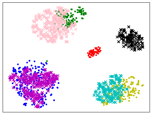
Figure 1: The data distribution map (better viewed in color) after training a classification model for an old task and then a new task. Many different relation data (different colors) of the old (dots) and new (crosses) task are mixed due to the catastrophic forgetting, making it hard to distinguish the new task’s relations from the old task’s relations.

Through our empirical studies, we found that the catastrophic forgetting of a model results in the indistinguishability between the data (instances) distributions of all tasks, making it hard to distinguish the relations of all tasks. We illustrate it with the data distribution map after training a relation classification model for a new task, as shown in Figure 1 where the dots and crosses represent the data of the old and new task respectively, and different colors represent different relations. It shows that the data points of different colors in either dot group (old task) or cross group (new task) are distinguishable. However, many dots and crosses are mixed, making it hard to discriminate the new task’s relations from the old task’s relations. Therefore, making the data distributions of all tasks more distinguishable is crucial to achieve better CRE.

To address above issue, in this paper we propose a novel Continual Relation Extraction framework with Contrastive Learning, namely CRECL, which is built with a classification network and a contrastive network. In order to fully leverage the information of negative relations to make the data distributions of all tasks more distinguishable, we design a prototypical contrastive learning scheme. Specifically, in the contrastive network of CRECL, a given instance is contrasted with the prototype of each candidate relation stored in the memory module. Such sufficient comparisons ensure the alignment and uniformity between the data distributions of old and new tasks. Therefore, the catastrophic forgetting in CRECL is alleviated more thoroughly, resulting in enhanced CRE performance. In addition, different to the classification for a fixed (relation) class set as Han et al. (2020); Cui et al. (2021), CRECL achieves an incremental-class learning of CRE which is more feasible to real-world CRE scenarios.

Our contributions in this paper are summarized as follows:

1. We propose a novel CRE framework CRECL that combines a classification network and a prototypical contrastive network to fully alleviate the problem of catastrophic forgetting.

2. With the contrasting-based mechanism, our CRECL can effectively achieve the class-incremental learning which is more practical in real-world CRE scenarios.

3. Our extensive experiments justify our CRECL’s advantage over the state-of-the-art (SOTA) models on two benchmark datasets, TACRED and FewRel. Furthermore, we provide our deep insights into the reasons of the compared models’ distinct performance.

2 Related Work

In this section, we briefly introduce continual learning and contrastive learning which are both related to our work.

Continual learning Delange et al. (2021); Parisi et al. (2019) focuses on the learning from a continuous stream of data. The models of continual learning are able to accumulate knowledge across different tasks without retraining from scratch. The major challenge in continual learning is to alleviate catastrophic forgetting which refers to that the performance on previous tasks should not significantly decline over time as new tasks come in. For overcoming catastrophic forgetting, most recent works can be divided into three categories. 1) Regularized-based methods impose constraints on the update of parameters. For example, LwF approach Li and Hoiem (2016) enforces the network of previously learned tasks to be similar to the network of current task by knowledge distillation. However, LwF depends heavily on the data in new task and its relatedness to prior tasks. EWC Kirkpatrick et al. (2016) adopts a quadratic penalty on the difference between the parameters for old and new tasks. It models the parameter relevance with respect to training data as a posterior distribution, which is estimated by Laplace approximation with the precision determined by the Fisher Information Matrix. WA Zhao et al. (2020) maintains discrimination and fairness among the new and old task by adjust the parameters of the last layer. 2) Dynamic architecture methods change models’ architectural properties upon new data by dynamically accommodating new neural resources, such as increased number of neurons. For example, PackNet Mallya and Lazebnik (2017) iteratively assigns parameter subsets to consecutive tasks by constituting pruning masks, which fixes the task parameter subset for future tasks. DER Yan et al. (2021) proposes a novel two-stage learning approach to get more effective dynamically expandable representation. 3) Memory-based methods explicitly retrain the models on a limited subset of stored samples during the training on new tasks. For example, iCaRL Rebuffi et al. (2017) focuses on learning in a class-incremental way, which selects and stores the samples most close to the feature mean of each class. During training, distillation loss between targets obtained from previous and current model predictions is added into overall loss, to preserve previously learned knowledge. RP-CRE Cui et al. (2021) introduces a novel pluggable attention-based memory module to automatically calculate old tasks’ weights when learning new tasks.

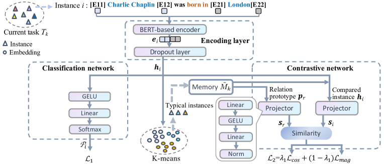
Figure 2: The overall structure of our proposed CRECL. The framework is built with a shared encoding layer, a classification network and a contrastive network.

Since classification-based approaches require relation schema in the classification layer, classification-based models have an unignorable drawback on class-incremental learning. Many researchers leverage metric learning to solve this problem. Wang et al. (2019); Wu et al. (2021) utilize sentence alignment model based on Margin Ranking Loss Nayyeri et al. (2019), while lack the intrinsic ability to perform hard positive/negative mining, resulting in poor performance. Recently, contrastive learning has been widely imported into self-supervised learning frameworks in many fields including computer vision, natural language processing and so on. Contrastive learning is a discriminative scheme that aims to group similar samples more closer and diverse samples far from each other. Wang and Liu (2021) proves that contrastive learning can promote the alignment and stability of data distribution, and Khosla et al. (2020) verifies that using modern batch contrastive approaches, such as InfoNCE loss Oord et al. (2018), outperforms traditional contrastive losses, such as margin ranking loss, and also achieves good results in supervised contrastive learning tasks.

3 Methodology

3.1 Task Formalization

The CRE task aims to identify the relation between two entities expressed by one sentence in the task sequence. Formally, given a sequence of $K$ tasks $\{T_{1},T_{2},\ldots,T_{K}\}$, suppose $D_{k}$ and $R_{k}$ denote the instance set and relation class set of the $k$-th task $T_{k}$, respectively. $D_{k}$ contains $N_{k}$ instances $\{(x_{1},t_{1},y_{1}),\ldots,(x_{N_{k}},t_{N_{k}},y_{N_{k}})\}$ where instance $(x_{i},t_{i},y_{i}),1\leq i\leq N_{k}$ represents that the relation of entity pair $t_{i}$ in sentence $x_{i}$ is $y_{i}\in{R}_{k}$. One CRE model should perform well on all historical tasks up to $T_{k}$, denoted as $\tilde{{T}}_{k}=\cup_{i=1}^{k}{T}_{i}$, of which the relation class set is $\tilde{{R}}_{k}=\cup_{i=1}^{k}{R}_{i}$. We also adopt an episodic memory module ${M}_{r}=\{(x_{1},t_{1},r),\ldots,(x_{L},t_{L},r)\}$ to store typical instances of relation $r$, similar to Han et al. (2020); Cui et al. (2021), where $L$ is the memory size (typical instance number). The overall episodic memory for the observed relations in all tasks is $\tilde{{M}}_{k}=\cup_{r\in\tilde{{R}}_{k}}{M}_{r}$.

3.2 Framework Overview

The overall structure of our CRECL is depicted in Figure 2, which has two major components, i.e., a classification network and a contrastive network. The procedure of learning the current task in CRECL is described by the algorithm in Alg. 1.

At first, suppose the current task is $T_{k}$, the representation of each instance in $T_{k}$ is obtained through the encoder and dropout layer shared by the two networks. In the classification network, each instance’s relation is predicted based on its representation (line 1-3). Then, we apply K-means algorithm over the instance representations to select $L$ typical instances for each relation in $T_{k}$, which are used to generate the relation prototypes and stored into memory $\tilde{M}_{k}$ for the subsequent contrast (line 4-13). There are two training processes in the contrastive network. The first is to compare current task instances with the stored relation prototypes of $\tilde{T}_{k}$ (line 14-17). The second is to compare each typical instance with all relation prototypes which are both stored in $\tilde{M}_{k}$ (line 18-24). These two training procedures ensure each compared instance keep distance from sufficient negative relations in $\tilde{R}_{k}$. Therefore, the data distributions of $\tilde{R}_{k}$ are distinguishable enough to alleviate CRECL’s catastrophic forgetting of old tasks. Next, we detail the operations in CRECL.

Input: $D_{k},R_{k},\tilde{R}_{k-1},\tilde{M}_{k-1}$

Output: $\tilde{M}_{k}$

1 for $i$ = 1 to epochs1 do

2       update Encoder $EN$, Dropout layer $DR$ and Classifier $CL$ by loss $\mathcal{L}_{1}$ on $D_{k}$;

3      

4 end for

5$\tilde{R}_{k}=\tilde{R}_{k-1}\cup R_{k}$;

6 $\boldsymbol{p}=\emptyset$;

7 for  $r\in R_{k}$ do

8       $d_{r}=\{d|d\in D_{k},y_{d}=r$};

9       $\boldsymbol{h}_{r}$=DR(EN($d_{r}$))//Eq. 1;

10       apply K-means to all $\boldsymbol{h}_{r}$ and store $L$ typical instances into memory $M_{k}$;

11       get prototype $\boldsymbol{p}_{r}$ from $M_{k}$ by Eq. 4;

12       $\boldsymbol{p}=\boldsymbol{p}\cup\boldsymbol{p}_{r}$;

13      

14 end for

15$\tilde{M}_{k}=\tilde{M}_{k-1}\cup M_{k}$;

16 generate contrastive training data $C_{k}$ by random sampling from $D_{k}$;

17 for $i$ = 1 to epochs2 do

18       update $EN$, $DR$, $PJ$ by loss $\mathcal{L}_{2}$ on $C_{k}$ and $\boldsymbol{p}$;

19      

20 end for

21generate contrastive training data $\tilde{C_{k}}$ by random sampling from $\tilde{M}_{k}$;

22 for $i$ = 1 to epochs3 do

23       if $y_{i}\in\tilde{C_{k}}$ is old class then

24             use Eq. 1 to generate M embeddings;

25            

26       end if

27      update $EN$, $DR$, $PJ$ by loss $\mathcal{L}_{2}$ on $\tilde{C_{k}}$ and $\boldsymbol{p}$;

28      

29 end for

Algorithm 1 Training procedure for $T_{k}$

3.3 Shared Encoding Layer

The classification network and the contrastive network in CRECL are designed to promote each other, where the former classifies the current task based on its instance embeddings, and the latter effectively adjusts instance embeddings to keep uniformity and alignment. According to this principle, the two networks share the same layers in CRECL.

Specifically, for an instance $i$ of current task $T_{k}$, we use special tokens to represent the entities in $i$ as Cui et al. (2021). As shown in Figure 2, the head entity and tail entity in $i$ are represented by two special position tokens $[E11,E12]$ and $[E21,E22]$, respectively. The embedding of instance $i$ before the dropout layer, denoted as $\boldsymbol{e}_{i}\in\mathbb{R}^{2h}$, is the concatenation of token embeddings of $[E11,E12]$ and $[E21,E22]$ generated by BERT Devlin et al. (2019) where $h$ is the dimension of two token embeddings. Then, $\boldsymbol{e}_{i}$ is fed into the dropout layer to obtain $i$’s hidden embedding as

$$\boldsymbol{h}_{i}=\big{(}\boldsymbol{W}\operatorname{Dropout}(\boldsymbol{e}_{i})+\boldsymbol{b}\big{)}\in\mathbb{R}^{d},$$ (1)

where $\boldsymbol{W}\in\mathbb{R}^{{d}\times{2h}}$ (d is dimension of hidden layer) and $\boldsymbol{b}\in\mathbb{R}^{d}$ are both trainable parameters. In CRECL, $\boldsymbol{h}_{i}$ is regarded as $i$’s representation.

3.4 Classifying Current Task

With instance $i$’s representation $\boldsymbol{h}_{i}$, $i$’s probability distribution denoted as $\mathcal{P}_{i}\in\mathbb{R}^{|R_{k}|}$, is calculated in the classification network as

$$\mathcal{P}_{i}=\operatorname{softmax}\big{(}\boldsymbol{W}_{1}\operatorname{LN}\big{(}\operatorname{GELU}(\boldsymbol{h}_{i})\big{)}+\boldsymbol{b}_{1}\big{)},$$ (2)

where $\boldsymbol{W}_{1}\in\mathbb{R}^{|R_{k}|\times{d}},\boldsymbol{b}_{1}\in\mathbb{R}^{|R_{k}|}$ are trainable parameters, and $|R_{k}|$ is the relation number of current task $T_{k}$ which is much less than the relation number of all tasks. $\operatorname{LN}(\cdot)$ is layer normalization operation. Then, classification loss for current task $T_{k}$ is calculated as

$$\mathcal{L}_{1}=-\frac{1}{N_{k}}\sum_{i=1}^{N_{k}}\sum_{r=1}^{|R_{k}|}y_{i,r}\log\mathcal{P}_{i}^{r},$$ (3)

where $y_{i,r}$=1 if $i$’s real relation label is $r$, otherwise $y_{i,r}$=0. $\mathcal{P}_{i}^{r}$ is the $r$-th entry in $\mathcal{P}_{i}$.

3.5 Generating Relation Prototypes

After learning current task, for each relation $r$ in current task, we first apply K-means algorithm upon the representations ($\boldsymbol{h}_{i}$) of all instances belonging to $r$ to cluster them into $L$ clusters. Then, for each cluster, we select the instance most closest to the centroid of this cluster as one typical instance. Thus, $L$ typical instances of relation $r$ are selected and then stored into the memory module. With the stored typical instances of $r$, we average their representations as $r$’s prototype $\boldsymbol{p}_{r}$, that is

$$\boldsymbol{p}_{r}=\frac{1}{L}\sum_{i=1}^{L}\boldsymbol{h}_{i}^{r},$$ (4)

where $\boldsymbol{h}_{i}^{r}$ is a typical instance $i$’s representation of relation $r$. Such prototype best represents $r$ since the $L$ typical instances have the minimal distance sum to the $L$ cluster centroids. Another merit of such prototypes for representing relations is their insensitivity to the value of $L$.

3.6 Contrastive Network

In this contrastive network, the instances are compared with the relation prototypes stored in the memory module to refine the data distributions of all tasks, so as to alleviate CRECL’s catastrophic forgetting. Its basic principle is that, an instance’s representation should be close to the prototype of its (positive) relation, and be far away from the prototypes of the rest (negative) relations. Please note that, the positive and negative relations are identified by the real labels of the training instances. Thus it is different from the self-supervised contrastive learning in other models Chen et al. (2020).

Contrastive Learning Objective

As shown in the right part of Figure 2, the contrastive network is built with a twin-tower architecture. In the left tower, for a relation $r$, its prototypes $\boldsymbol{p}_{r}\in\mathbb{R}^{d}$ are obtained by Eq. 4. Then, $r$’s compared embedding is denoted as $\boldsymbol{s}_{r}\in\mathbb{R}^{\frac{d}{2}}$ and computed as

$$\boldsymbol{s}_{r}=\boldsymbol{W}_{3}\operatorname{GELU}(\boldsymbol{W}_{2}\boldsymbol{p}_{r}+\boldsymbol{b}_{2})+\boldsymbol{b}_{3},$$ (5)

where $\boldsymbol{W}_{2}\in\mathbb{R}^{{d}\times{d}}$, $\boldsymbol{b}_{2}\in\mathbb{R}^{d}$, $\boldsymbol{W}_{3}\in\mathbb{R}^{\frac{d}{2}\times{d}}$, $\boldsymbol{b}_{3}\in\mathbb{R}^{\frac{d}{2}}$ are both trainable parameters.

In the right tower, for a compared instance $i$, its compared embedding is denoted as $\boldsymbol{s}_{i}\in\mathbb{R}^{\frac{d}{2}}$ and obtained by the same operation in Eq. 5 where only $\boldsymbol{p}_{r}$ is replaced by $\boldsymbol{h}_{i}$ from Eq. 1.

For each instance $i$ in current task $T_{k}$, suppose the compared embedding of $i$’s relation $y_{i}$ is $\boldsymbol{s}_{y_{i}}$ which can also be obtained by Eq. 5, since the typical instances of $y_{i}$ have been stored in $\tilde{M}_{k}$ before. We apply Euclidean norm to $\boldsymbol{s}_{i}$ and $\boldsymbol{s}_{y_{i}}$. Then, we use contrastive learning’s InfoNCE loss Oord et al. (2018) to calculate the cosine similarity loss of $T_{k}$ as

$$\mathcal{L}_{cos}=-\frac{1}{N_{k}}\sum_{i=1}^{N_{k}}\log\frac{\exp\left(\boldsymbol{s}_{i}\boldsymbol{s}_{y_{i}}/\tau\right)}{\sum\limits_{r\in\tilde{R}_{k}}\exp\left(\boldsymbol{s}_{i}\boldsymbol{s}_{r}/\tau\right)},$$ (6)

where $\tau$ is a temperature hyper-parameter.

To increase the similarity score gap of the correct label and the closest wrong label, inspired by Koch et al. (2015), we propose a contrastive margin loss

$$\mathcal{L}_{mag}=\frac{1}{N_{k}}\sum_{i=1}^{N_{k}}max\big{(}m-\boldsymbol{s}_{i}\boldsymbol{s}_{y_{i}}+\boldsymbol{s}_{i}\boldsymbol{s}_{k_{i}},0\big{)},$$ (7)

where relation $k_{i}=\mathop{\arg\max}\limits_{k\in\tilde{R}_{k}}\boldsymbol{s}_{i}\boldsymbol{s}_{k}$ s.t. $k\neq y_{i}$, that is $i$’s closest negative relation label. The margin loss penalizes that the similarity gap less than $m$. At last, the total loss is defined as

$$\mathcal{L}_{2}=\lambda_{1}\mathcal{L}_{cos}+(1-\lambda_{1})\mathcal{L}_{mag},$$ (8)

where $\lambda_{1}\in[0,1]$ is the controlling parameter.

Training Processes of Contrastive Learning

There are two training processes in the contrastive network, which both use the loss in Eq. 8 to make the network parameters more fit to current task and all historical tasks, respectively.

The first training process is conducted with current task $T_{k}$ and complements the classification network, it is an optional step with relatively small training epoch. However, it can not ensure the model fit to all tasks, because the model pays more attention to current task rather than the old tasks during this training process. In other words, as we have explained in the example of Figure 1, the model tends to ensure the instances of different relations in $T_{k}$ distinguishable, but forgets to meanwhile keep the instances of different relations in all historical tasks also distinguishable. As a result, the model’s catastrophic forgetting still happens.

To alleviate CRECL’s catastrophic forgetting more thoroughly, we introduce the second training process in the contrastive network. In this process, all typical instances stored in the memory module are compared with all prototypes of stored relations, which cover in all tasks. We also conduct $M$ times forward propagation in the dropout layer, to generate $M$ embeddings for each old relation in $\tilde{R}_{k-1}$. Due to the randomness of dropout layer, we can get $M$ probability distributions for an old relation to reduce the imbalance of data distribution of old and new relation. Accordingly, this training process can effectively prevent the model from severe catastrophic forgetting.

3.7 Relation Prediction

For a predicted instance $i$, we only measure its similarity to each stored relation, which is computed as the cosine distance between $i$’s representation and the relation’s prototype. Then, we choose the most similar (closest) relation as $i$’s predicted class label, that is

$$y^{*}_{i}=\mathop{\arg\max}\limits_{r\in\tilde{{R}}_{k}}\boldsymbol{s}_{i}\boldsymbol{s}_{r}.$$ (9)

4 Experiments

Table 1: Accuracy (%) comparisons on different test sets of historical cumulative tasks, showing that CRECL outperforms the compared models.

	FewRel
Model	T1	T2	T3	T4	T5	T6	T7	T8	T9	T10
EA-EMR	89.0	69.0	59.1	54.2	47.8	46.1	43.1	40.7	38.6	35.2
EMAR	88.5	73.2	66.6	63.8	55.8	54.3	52.9	50.9	48.8	46.3
CML	91.2	74.8	68.2	58.2	53.7	50.4	47.8	44.4	43.1	39.7
EMAR+BERT	98.8	89.1	89.5	85.7	83.6	84.8	79.3	80.0	77.1	73.8
RP-CRE+MA	98.0	91.4	91.8	86.8	87.6	86.9	83.7	81.9	80.1	79.5
RP-CRE	97.9	92.7	91.6	89.2	88.4	86.8	85.1	84.1	82.2	81.5
CRECL+ATM(Ours)	96.3	91.4	89.3	90.0	88.1	86.7	84.5	83.2	82.6	81.0
CRECL(Ours)	97.8	94.9	92.7	90.9	89.4	87.5	85.7	84.6	83.6	82.7
Improvement(%)	-1.01	2.37	0.98	1.91	1.13	0.69	0.71	0.59	1.70	1.47
	TACRED
Model	T1	T2	T3	T4	T5	T6	T7	T8	T9	T10
EA-EMR	47.5	40.1	38.3	29.9	28.4	27.3	26.9	25.8	22.9	19.8
EMAR	73.6	57.0	48.3	42.3	37.7	34.0	32.6	30.0	27.6	25.1
CML	57.2	51.4	41.3	39.3	35.9	28.9	27.3	26.9	24.8	23.4
EMAR+BERT	96.6	85.7	81.0	78.6	73.9	72.3	71.7	72.2	72.6	71.0
RP-CRE+MA	97.1	91.4	87.4	82.1	78.3	77.8	74.9	73.5	73.6	72.3
RP-CRE	97.6	90.6	86.1	82.4	79.8	77.2	75.1	73.7	72.4	72.4
CRECL+ATM(Ours)	93.2	80.2	77.3	76.0	71.8	71.5	69.2	72.3	70.0	71.2
CRECL(Ours)	96.6	93.1	89.7	87.8	85.6	84.3	83.6	81.4	79.3	78.5
Improvement(%)	-1.02	1.86	2.63	6.55	7.27	8.35	11.32	10.45	7.74	8.43

4.1 Datasets

Our experiments were conducted upon the following two benchmark CRE datasets.

FewRel Han et al. (2018) is a popular relation extraction dataset originally constructed for few-shot relation extraction. The dataset is annotated by crowd workers and contains 100 relations and 70,000 samples in total. In our experiments, to keep consistent with the previous baselines, we used its version of 80 relations.

TACRED Zhang et al. (2017) is a large-scale relation extraction dataset containing 42 relations (including no_relation) and 106,264 samples from news and web documents. Based on the open relation assumption of CRE, we removed no_relation in our experiments. To limit the sample imbalance of TACRED, we limited the number of training samples of each relation to 320, and the number of test samples of each relation to 40, which is also consistent with previous baselines. Compared with FewRel, the tasks in TACRED are more difficult due to its relation imbalance and semantic difficulty.

4.2 Compared Models

We compare our framework with the following baselines in our experiments.

EA-EMR Wang et al. (2019) proposes a sentence alignment model with replay memory module to alleviate catastrophic forgetting.

EMAR Han et al. (2020) proposes a novel memory replay, activation and reconsolidation method to alleviate catastrophic forgetting effectively.

EMAR+BERT is an advanced version of EMAR where the original encoder (Bi-LSTM) is replaced with BERT.

CML Wu et al. (2021) proposes a curriculum-meta learning method to tackle the order-sensitivity and catastrophic forgetting in CRE.

RP-CRE Cui et al. (2021) is a SOTA CRE model introducing a novel pluggable attention-based memory module to automatically calculate the weight of old tasks when learning new tasks.

RP-CRE+MA is an advanced version of RP-CRE where a memory activation step is added before attention operation.

In our CRECL, we adopted the Bert-base-uncased pre-trained by HuggingFace Wolf et al. (2020) as the encoder, which is also used in EMAR+BERT, RP-CRE and RP-CRE+MA. Other baselines cannot be easily replaced by the BERT due to their architectures. In addition, we propose another version of CRECL, namely CRECL+ATM, which incorporates an attention memory module proposed by Cui et al. (2021) in the contrastive network and used to verify its effectiveness of refining relation prototypes.

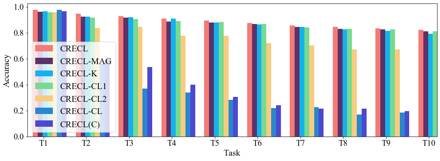
(a) Accuracy of historical cumulative tasks on FewRel.

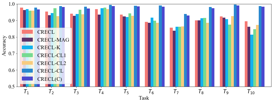
(b) Accuracy of current task on FewRel.

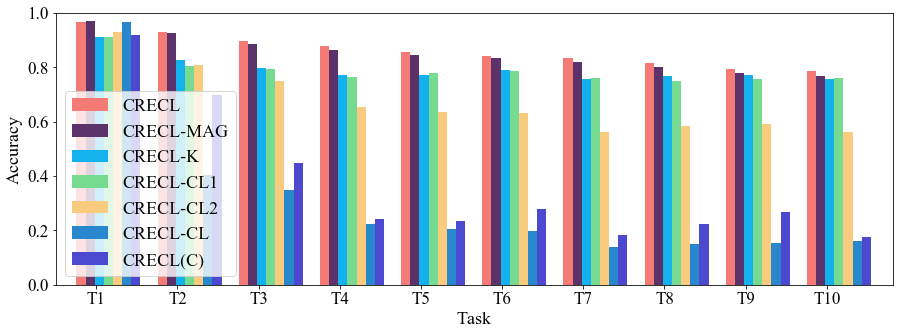
(c) Accuracy of historical cumulative tasks on TACRED.

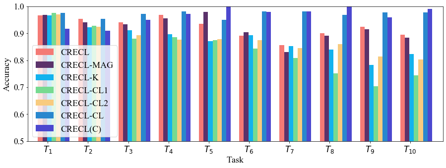
(d) Accuracy of current task on TACRED.

Figure 3: Ablation study results on historical cumulative tasks and current task.

4.3 Experimental Settings

Our evaluation metric is Accuracy which is popularly used in previous baselines.

For fair comparisons, we followed the experiment settings in RP-CRE. At first, to verify whether a CRE model suffers from catastrophic forgetting, we use $Tk$ to represent the test set of all historical cumulative tasks from the first task to the $k$-th task $T_{k}$ (Please note the difference between $Tk$ and $T_{k}$). In our ablation studies, we also report the performance on the test set of current task. To simulate different tasks, we randomly divided all instances into 10 groups (corresponding to 10 tasks). The task order of all compared models is exactly the same to reduce contingency. We also set the memory size in the baselines the same as ours. Relations are first divided into 10 clusters to simulate 10 tasks. All the reported results of the related baselines are the same as Cui et al. (2021). For those special hyper-parameters in our experiments are as follows. The batch size is 32, the learning rate is set to 5e-5, $\tau$ is 0.08. We adopted 10 and 15 classification epochs for TACRED and FewRel, respectively. We also adopted 10 epochs for the first training process (for current task) and 5 epochs for the second training process (for all tasks) in the contrastive network.

Because the total matrix operations and the data amount of second training in contrastive learning are very small, CRECLl’s training time (1h31min) is very close to the SOTA model RP-CRE (1h28min). To reproduce our experiment results conveniently, CRECL’s source code together with the datasets are provided at https://github.com/PaperDiscovery/CRECL.

4.4 Experimental Results and Analyses

The following reported results of CRECL and its ablated variants are the average scores of running models for 5 times.

4.4.1 Overall Performance Comparisons

The overall performance of all compared baselines are reported in Table 1, where the results of the baselines directly come from Cui et al. (2021) and the baselines’ hyper-parameter settings were the same as their original papers. The last row in the table is the improvement ratio of CRECL’s performance relative to the best baseline’s performance (underline). Based on these results, we have the following conclusions:

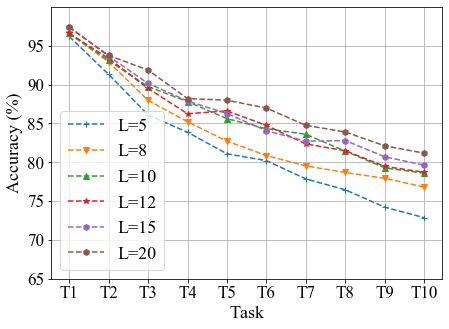
(a) CRECL

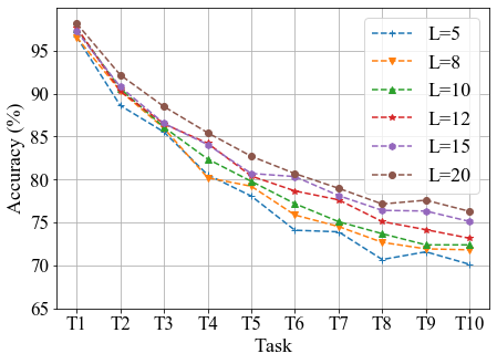
(b) RP-CRE

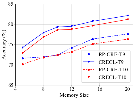
(c) CRECL vs. RP-CRE in T9/T10

Figure 4: Performance comparisons with different memory sizes on TACRED.

(1) Our CRECL outperforms the SOTA model RP-CRE on both datasets. Compared with FewRel, CRECL has more apparent improvement over the baselines on TACRED. This may be due to that FewRel’s tasks are not difficult enough as TACRED, proving that CRECL is good at handling more difficult tasks.

(2) In T1, our CRECL is inferior to RP-CRE because the classification and contrastive network in CRECL have not been fully trained at the beginning. When more tasks are cumulated, CRECL is trained sufficiently, resulting in its superiority over the baselines and less performance drop. Since the catastrophic forgetting becomes more severe on such scenarios, the results imply that CRECL can tackle the catastrophic forgetting better.

(3) All compared models’ performance is well on T1, but declines when more new tasks arrive due to more severe catastrophic forgetting. Compared with EA-EMR, EMAR and CML, the rest models’ performance decline is more slight. For example, from the comparison between EMAR (using Bi-LSTM) and EMAR+BERT, we can see that EMAR+BERT’s performance decline significantly slows down, proving that BERT helps the model alleviate the catastrophic forgetting better. It is because BERT has good feature discrimination ability and better captures the relevant features, making catastrophic forgetting less severe.

(4) CREL+ATM’s results show that incorporating attention memory module fails to improve CRECL’s performance well, because the contrastive network is able to maintain the uniformity and the alignment of data distribution. Thus there is no need for additional attention memory module to help the model refine relation prototypes.

(5) Compared with the models using metric learning (EA-EMR, EMAR, CML, EMAR+BERT), we adopt InfoNCE loss instead of the margin ranking loss as our loss function. With this loss, CRECL is taught by more negative relation information to understand how to regularize data representation space, resulting in the more alleviation of catastrophic forgetting.

Table 2: Our framework’s accuracy (%) with different memory sizes on FewRel.

CRECL	T1	T2	T3	T4	T5	T6	T7	T8	T9	T10
$L$=5	97.1	92.1	89.7	90.0	88.2	86.6	84.4	82.8	82.5	80.2
$L$=10	97.8	94.9	92.7	90.9	89.4	87.5	85.7	84.6	83.6	82.7
$L$=15	98.9	96.3	93.8	92.6	91.4	90.0	88.0	86.6	85.8	83.5
$L$=20	98.1	96.0	94.1	92.8	91.9	89.7	88.5	86.3	86.1	85.2

4.4.2 Ablation Studies

In order to verify the effectiveness and rationality of our framework’s important components (steps), we further conducted a series of ablation experiments. CRECL’s ablated variants include:

CRECL-MAG: It is the variant without the margin loss $\mathcal{L}_{mag}$ in the contrastive network.

CRECL-CL1: It is the variant without the first training process in the contrastive network.

CRECL-CL2: It is the variant without the second training process in the contrastive network.

CRECL-CL: It is the variant only having the classification network.

CRECL-K: In this variant, the typical instances of each relation are selected at random instead of by K-means algorithm.

CRECL(C): This variant uses the classification network to identify the relation of a test instance instead of the similarity comparison in Eq. 9.

Figure 3 (a) and (b) display all compared models’ accuracy of historical cumulative tasks and current task. Due to space limitation, only the results on TACRED are shown, based on which we have the following analyses.

(1) CRECL-CL performs very well on current task (subfigure (b)) but performs very poorly on historical tasks (subfigure (a)), showing that it overfits current task and its catastrophic forgetting is very severe. It is because that the classification parameters are always tuned to fit with current task rather than old tasks. It shows that the contrastive network is significant to alleviate catastrophic forgetting.

(2) As more new tasks arrive, CRECL-CL1’s performance decline on current task (subfigure (b)) is more obvious than its performance decline on historical tasks (subfigure (a)), because CRECL-CL1 pays more attention to distinguish the different relations in old tasks rather than that in current task. It is due to that the data distributions of all historical tasks are adjusted in the second training process that CRECL-CL1 only has in its contrastive network. Comparatively, CRECL-CL2’s performance on historical tasks and current task both declines. It shows that only distinguishing the data distribution of current task from that of old tasks in the first training process of contrastive network, is not adequate to alleviate its catastrophic forgetting. Even worse, such adjusting also harms the accuracy of classifying current task.

(4) CRECL-K is inferior to CRECL, showing that the randomly selected instances cannot well represent relations as those selected by K-means algorithm. As a result, the data distributions of all tasks cannot be adjusted precisely, which can not alleviate catastrophic forgetting effectively. In addition, CRECL-K’s accuracy on current task is not stable also due to the randomness led by its selection strategy of typical instances.

(5) Although the contrastive learning loss $\mathcal{L}_{2}$ is different from the classification network’s loss $\mathcal{L}_{1}$, and the parameters of the encoding layer are shared, the contrastive network’s training processes hardly weaken the classification network’s fitness to current task. Thus CRECL(C) still performs well on current task as shown in Figure 3 (b). CRECL-MAG’s has a relatively small decline on both current and historical tasks, proving that the margin loss $\mathcal{L}_{mag}$ improves the performance by increasing the gap between the optimal and suboptimal results.

4.4.3 Performance Influence of Memory Size

For memory-based CRE methods, the model performance is usually related to the storage capacity of their memory modules. Specifically, we found that previous models’ performance is very sensitive to the number of stored typical instances $L$. Recall that in CRECL, a relation prototype is the average of $L$ typical instances’ representations. The representational ability of such prototype is less sensitive to $L$ when $L$ exceeds a certain value, resulting in CRECL’s performance also less sensitive to $L$, as we emphasized in Section 3.5.

Figure 4 displays the performance of CRECL and RP-CRE on TACRED w.r.t. different memory sizes ($L$), where the two compared models’ performance in T9 and T10 is specially shown in the subfigure (c). It shows that although CRECL’s performance also declines when $L$ becomes small, it is more stable and higher than RP-CRE’s performance, especially when $L\geq 8$. Such results justifies our claim about CRECL’s less sensitivity to $L$. In addition, RP-CRE’s performance fluctuation is more obvious, possibly because it re-constructs the attention memory network upon each task, so the different task features are not shared in the network.

4.4.4 Contrastive Learning’s Effectiveness on Refining Data Distributions

In addition, to investigate the contrastive learning’s effects on alleviating catastrophic forgetting, we use t-SNE Van der Maaten and Hinton (2008) to visualize the data distributions of the same case in Figure 1 after the training processes of CRECL’s classification network and contrastive network. The data distribution map is shown in Figure 5, which has the same settings of color and point style as Figure 1. Through comparing these two maps, we find that the data distributions of different relations in the new and old task in Figure 5 are more distinguishable than that in Figure 1. Such results are mainly attributed to the prototypical contrastive learning in CRECL on adjusting all data distributions of all tasks, which obviously alleviate CRECL’s catastrophic forgetting. It has been also proved by CRECL’s superior performance over the baselines displayed in aforementioned experiments. We also note that some yellow dots still intersect the pink crosses, possibly due to the insufficient sampling in the contrastive learning, resulting in less coverage on all relations. We can handle this situation by increasing the batch size.

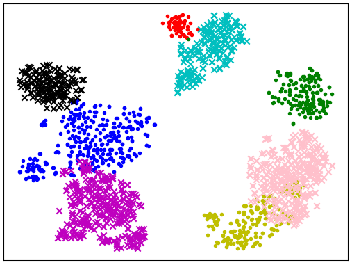
Figure 5: Data distribution map (better viewed in color) after the contrastive learning in CRECL. Compared with Fig. 1, the data distributions of different relations (different colors) are obviously distinguishable, making CRECL classify different relations more easily.

5 Conclusion

In this paper, we propose a novel CRE framework, namely CRECL, that consists of a classification network and a contrastive network designed for alleviating the catastrophic forgetting in CRE. Through the prototypical contrastive learning in CRECL, the data distributions of different relations in all tasks are adjusted to be more distinguishable, resulting in CRE performance gains. Moreover, CRECL has the ability of class-incremental learning due to its contrasting-based mechanism of achieving relation classification, which is more practical in real-world CRE scenarios than the previous models of classification-based mechanism. Our extensive experimental results demonstrate that CRECL outperforms the SOTA CRE baselines and obtains the best performance on two benchmark datasets.

References

- Chaudhry et al. (2018) Arslan Chaudhry, Marc’Aurelio Ranzato, Marcus Rohrbach, and Mohamed Elhoseiny. 2018. Efficient lifelong learning with a-gem. arXiv preprint arXiv:1812.00420.
- Chen et al. (2015) Tianqi Chen, Ian Goodfellow, and Jonathon Shlens. 2015. Net2net: Accelerating learning via knowledge transfer. arXiv preprint arXiv:1511.05641.
- Chen et al. (2020) Ting Chen, Simon Kornblith, Mohammad Norouzi, and Geoffrey Hinton. 2020. A simple framework for contrastive learning of visual representations. In International conference on machine learning, pages 1597–1607. PMLR.
- Cui et al. (2021) Li Cui, Deqing Yang, Jiaxin Yu, Chengwei Hu, and et al. 2021. Refining sample embeddings with relation prototypes to enhance continual relation extraction. In Proceedings of the 59th Annual Meeting of the Association for Computational Linguistics, pages 232–243.
- Delange et al. (2021) Matthias Delange, Rahaf Aljundi, Marc Masana, Sarah Parisot, Xu Jia, Ales Leonardis, Greg Slabaugh, and Tinne Tuytelaars. 2021. A continual learning survey: Defying forgetting in classification tasks. IEEE Transactions on Pattern Analysis and Machine Intelligence, pages 1–1.
- Devlin et al. (2019) Jacob Devlin, Ming-Wei Chang, Kenton Lee, and Kristina Toutanova. 2019. BERT: pre-training of deep bidirectional transformers for language understanding. In Proceedings of NAACL, pages 4171–4186.
- Fernando et al. (2017) Chrisantha Fernando, Dylan Banarse, Charles Blundell, Yori Zwols, David Ha, Andrei A Rusu, Alexander Pritzel, and Daan Wierstra. 2017. Pathnet: Evolution channels gradient descent in super neural networks. arXiv preprint arXiv:1701.08734.
- Han et al. (2020) Xu Han, Yi Dai, Tianyu Gao, Yankai Lin, Zhiyuan Liu, Peng Li, Maosong Sun, and Jie Zhou. 2020. Continual relation learning via episodic memory activation and reconsolidation. In Proceedings of ACL, pages 6429–6440.
- Han et al. (2018) Xu Han, Hao Zhu, Pengfei Yu, Ziyun Wang, Yuan Yao, Zhiyuan Liu, and Maosong Sun. 2018. Fewrel: A large-scale supervised few-shot relation classification dataset with state-of-the-art evaluation. arXiv preprint arXiv:1810.10147.
- Hassabis et al. (2017) Demis Hassabis, Dharshan Kumaran, Christopher Summerfield, and Matthew Botvinick. 2017. Neuroscience-inspired artificial intelligence. Neuron, 95(2):245–258.
- Khosla et al. (2020) Prannay Khosla, Piotr Teterwak, Chen Wang, Aaron Sarna, Yonglong Tian, Phillip Isola, Aaron Maschinot, Ce Liu, and Dilip Krishnan. 2020. Supervised contrastive learning. arXiv preprint arXiv:2004.11362.
- Kirkpatrick et al. (2017) James Kirkpatrick, Razvan Pascanu, Neil Rabinowitz, Joel Veness, Guillaume Desjardins, Andrei A Rusu, Kieran Milan, John Quan, Tiago Ramalho, Agnieszka Grabska-Barwinska, et al. 2017. Overcoming catastrophic forgetting in neural networks. Proceedings of the national academy of sciences, 114(13):3521–3526.
- Kirkpatrick et al. (2016) James Kirkpatrick, Razvan Pascanu, Neil C. Rabinowitz, Joel Veness, and et al. 2016. Overcoming catastrophic forgetting in neural networks. CoRR, abs/1612.00796.
- Koch et al. (2015) Gregory Koch, Richard Zemel, Ruslan Salakhutdinov, et al. 2015. Siamese neural networks for one-shot image recognition. In ICML deep learning workshop, volume 2, page 0. Lille.
- Li and Hoiem (2016) Zhizhong Li and Derek Hoiem. 2016. Learning without forgetting. CoRR, abs/1606.09282.
- Mallya and Lazebnik (2017) Arun Mallya and Svetlana Lazebnik. 2017. Packnet: Adding multiple tasks to a single network by iterative pruning. CoRR, abs/1711.05769.
- Nayyeri et al. (2019) Mojtaba Nayyeri, Xiaotian Zhou, Sahar Vahdati, Hamed Shariat Yazdi, and Jens Lehmann. 2019. Adaptive margin ranking loss for knowledge graph embeddings via a correntropy objective function. arXiv preprint arXiv:1907.05336.
- Oord et al. (2018) Aaron van den Oord, Yazhe Li, and Oriol Vinyals. 2018. Representation learning with contrastive predictive coding. arXiv preprint arXiv:1807.03748.
- Parisi et al. (2019) German I. Parisi, Ronald Kemker, Jose L. Part, Christopher Kanan, and Stefan Wermter. 2019. Continual lifelong learning with neural networks: A review. Neural Networks, 113:54–71.
- Rebuffi et al. (2017) Sylvestre-Alvise Rebuffi, Alexander Kolesnikov, Georg Sperl, and Christoph H. Lampert. 2017. icarl: Incremental classifier and representation learning. In 2017 IEEE Conference on Computer Vision and Pattern Recognition, pages 5533–5542.
- Thrun and Mitchell (1995) Sebastian Thrun and Tom M Mitchell. 1995. Lifelong robot learning. Robotics and autonomous systems, 15(1-2):25–46.
- Van der Maaten and Hinton (2008) Laurens Van der Maaten and Geoffrey Hinton. 2008. Visualizing data using t-sne. Journal of machine learning research, 9(11).
- Wang and Liu (2021) Feng Wang and Huaping Liu. 2021. Understanding the behaviour of contrastive loss. In Proceedings of the IEEE/CVF Conference on Computer Vision and Pattern Recognition, pages 2495–2504.
- Wang et al. (2019) Hong Wang, Wenhan Xiong, Mo Yu, Xiaoxiao Guo, Shiyu Chang, and William Yang Wang. 2019. Sentence embedding alignment for lifelong relation extraction. In Proceedings of the 2019 Conference of the North American Chapter of the Association for Computational Linguistics: Human Language Technologies, pages 796–806.
- Wolf et al. (2020) Thomas Wolf, Lysandre Debut, Victor Sanh, and et al. 2020. Transformers: State-of-the-art natural language processing. In Proceedings of EMNLP, pages 38–45.
- Wu et al. (2021) Tongtong Wu, Xuekai Li, Yuan-Fang Li, Gholamreza Haffari, Guilin Qi, Yujin Zhu, and Guoqiang Xu. 2021. Curriculum-meta learning for order-robust continual relation extraction. pages 10363–10369.
- Yan et al. (2021) Shipeng Yan, Jiangwei Xie, and Xuming He. 2021. Der: Dynamically expandable representation for class incremental learning. In Proceedings of the IEEE/CVF Conference on Computer Vision and Pattern Recognition, pages 3014–3023.
- Zhang et al. (2017) Yuhao Zhang, Victor Zhong, Danqi Chen, Gabor Angeli, and Christopher D. Manning. 2017. Position-aware attention and supervised data improve slot filling. In Proceedings of EMNLP, pages 35–45.
- Zhao et al. (2020) Bowen Zhao, Xi Xiao, Guojun Gan, Bin Zhang, and Shu-Tao Xia. 2020. Maintaining discrimination and fairness in class incremental learning. In Proceedings of the IEEE/CVF Conference on Computer Vision and Pattern Recognition, pages 13208–13217.