Numerical stability and efficiency of response property calculations in density functional theory

Abstract.

Response calculations in density functional theory aim at computing the change in ground-state density induced by an external perturbation. At finite temperature these are usually performed by computing variations of orbitals, which involve the iterative solution of potentially badly-conditioned linear systems, the Sternheimer equations. Since many sets of variations of orbitals yield the same variation of density matrix this involves a choice of gauge. Taking a numerical analysis point of view we present the various gauge choices proposed in the literature in a common framework and study their stability. Beyond existing methods we propose a new approach, based on a Schur complement using extra orbitals from the self-consistent-field calculations, to improve the stability and efficiency of the iterative solution of Sternheimer equations. We show the success of this strategy on nontrivial examples of practical interest, such as Heusler transition metal alloy compounds, where savings of around 40% in the number of required cost-determining Hamiltonian applications have been achieved.

1. Introduction

Kohn-Sham (KS) density-functional theory (DFT) [26, 32] is the most popular approximation to the electronic many-body problem in quantum chemistry and materials science. While not perfect, it offers a favourable compromise between accuracy and computational efficiency for a vast majority of molecular systems and materials. In this work, we focus on KS-DFT approaches aiming at computing electronic ground-state (GS) properties. Having solved the minimization problem underlying DFT directly yields the ground-state density and corresponding energy. However, many quantities of interest, such as interatomic forces, (hyper)polarizabilities, magnetic susceptibilities, phonons spectra, or transport coefficients, correspond physically to the response of GS quantities to a change in external parameters (e.g. nuclear positions, electromagnetic fields). As such their mathematical expressions involve derivatives of the obtained GS solution with respect to these parameters. For example interatomic forces are first-order derivatives of the GS energy with respect to the atomic positions, and can actually be obtained without computing the derivatives of the GS density, thanks to the Hellmann-Feynman theorem [21]. On the other hand the computation of any property corresponding to second- or higher-order derivatives of the GS energy does require the computation of derivatives of the density. More precisely, it follows from Wigner’s $(2n+1)$ theorem that $n^{\rm th}$-order derivatives of the GS density are required to compute properties corresponding to $(2n)^{\rm th}$- and $(2n+1)^{\rm st}$-derivatives of the KS energy functional. More recent applications, such as the design of machine-learned exchange-correlation energy functionals, also require the computation of derivatives of the ground-state with respect to parameters, such as the ones defining the exchange-correlation functional [27, 29, 34].

Efficient numerical methods for evaluating these derivatives are therefore needed. The application of generic perturbation theory to the special case of DFT is known as density-functional perturbation theory (DFPT) [2, 15, 16, 18]. See also [37] for applications to quantum chemistry, [1] for applications to phonon calculations, and [9] for a mathematical analysis of DFPT within the reduced Hartree-Fock (rHF) approximation (also called the Hartree approximation in the physics literature). Although the practical implementation of first- and higher-order derivatives computed by DFPT in electronic structure calculation software can be greatly simplified by Automatic Differentiation techniques [19], the efficiency of the resulting code crucially depends on the efficiency of a key building block: the computation of the linear response $\delta\rho$ of the GS density to an infinitesimal variation $\delta V$ of the total Kohn-Sham potential.

For reasons that will be detailed below, the numerical evaluation of the linear map $\delta V\mapsto\delta\rho$ is not straightforward, especially for periodic metallic systems. Indeed, DFT calculations for metallic systems usually require the introduction of a smearing temperature $T$, a numerical parameter which has nothing to do with the physical temperature (in practice, its value is often higher than the melting temperature of the crystal). For the sake of simplicity, let us first consider the case of a periodic simulation cell $\Omega$ containing an even number $N_{\rm el}$ of electrons in a spin-unpolarized state (see Remark 1 for details on how this formalism allows for the computation of properties of perfect crystals). The Kohn-Sham GS at finite temperature $T>0$ is then described by an ${\rm L}^{2}(\Omega)$-orthonormal set of orbitals $(\phi_{n})_{n\in{\mathbb{N}}^{*}}$ with energies $(\varepsilon_{n})_{n\in{\mathbb{N}}^{*}}$, which are the eigenmodes of the Kohn-Sham Hamiltonian $H$ associated with the GS density:

$$H\phi_{n}=\varepsilon_{n}\phi_{n},\qquad\int_{\Omega}\phi_{m}^{*}(\bm{r})\phi_{n}(\bm{r}){\rm d}\bm{r}=\delta_{mn},\qquad\varepsilon_{1}\leqslant\varepsilon_{2}\leqslant\varepsilon_{3}\leqslant\cdots,$$

together with periodic boundary conditions. The GS density in turn reads

$$\rho(\bm{r})=\sum_{n=1}^{+\infty}f_{n}\mathopen{}\mathclose{{}\left|\phi_{n}(\bm{r})}\right|^{2}\quad\text{with}\quad f_{n}\coloneqq f\mathopen{}\mathclose{{}\left(\frac{\varepsilon_{n}-\varepsilon_{\rm F}}{T}}\right),$$ (1)

where $f$ is a smooth occupation function converging to $2$ at $-\infty$ and to zero at $+\infty$, e.g. the Fermi-Dirac smearing function $f(x)=\frac{2}{1+{\rm e}^{x}}$ (see Figure 1). The Fermi level $\varepsilon_{\rm F}$ is the Lagrange multiplier of the neutrality charge constraint: it is the unique real number such that

$$\int_{\Omega}\rho(\bm{r}){\rm d}\bm{r}=\sum_{n=1}^{+\infty}f_{n}=\sum_{n=1}^{+\infty}f\mathopen{}\mathclose{{}\left(\frac{\varepsilon_{n}-\varepsilon_{\rm F}}{T}}\right)=N_{\rm el}.$$

It follows from perturbation theory that the linear response $\delta\rho$ of the density to an infinitesimal variation $\delta V$ of the total Kohn-Sham potential is given by

$$\delta\rho=\chi_{0}\delta V,$$

where $\chi_{0}$ is the independent-particle susceptibility operator (also called noninteracting density response function). Equivalently, this operator describes the linear response of a system of noninteracting electrons of density $\rho$ subject to an infinitesimal perturbation $\delta V$. It holds (see Section 3)

$$\delta\rho(\bm{r})\coloneqq(\chi_{0}\delta V)(\bm{r})=\sum_{n=1}^{+\infty}\sum_{m=1}^{+\infty}\frac{f_{n}-f_{m}}{\varepsilon_{n}-\varepsilon_{m}}\phi_{n}^{*}(\bm{r})\phi_{m}(\bm{r})\mathopen{}\mathclose{{}\left(\delta V_{mn}-\delta\varepsilon_{\rm F}\delta_{mn}}\right),$$ (2)

where $\delta V_{mn}\coloneqq\mathopen{}\mathclose{{}\left\langle\phi_{m},\delta V\phi_{n}}\right\rangle$, $\delta\varepsilon_{\rm F}$ is the induced variation of the Fermi level $\varepsilon_{\rm F}$, and $\delta_{mn}$ is the Kronecker symbol. We also use the convention $(f_{n}-f_{n})/(\varepsilon_{n}-\varepsilon_{n})=\frac{1}{T}f^{\prime}\mathopen{}\mathclose{{}\left(\frac{\varepsilon_{n}-\varepsilon_{\rm F}}{T}}\right)$.

In practice, these equations are discretized on a finite basis set, so that the sums in (1) and (2) become finite. Since the number of basis functions $N_{\rm b}$ is often very large compared to the number of electrons in the system, it is very expensive to compute the sums as such. However, in practice it is possible to restrict to the computation of a number $N\ll N_{\rm b}$ of orbitals. These orbitals are then computed using efficient iterative methods [38].

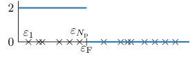
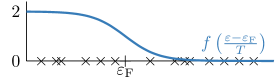
Figure 1. The occupation numbers $f_{n}$ for $T=0$ (left) and $T>0$ (right).

For insulating systems, there is a (possibly) large band gap between $\varepsilon_{N_{\rm p}}$ and $\varepsilon_{N_{\rm p}+1}$ which remains non-zero in the thermodynamic limit of a growing simulation cell. As a result, the calculation can be done at zero temperature, such that the occupation function $f$ becomes a step function (see Figure 1). The jump from $2$ to $0$ in the occupations occurs exactly when the lowest $N_{\rm p}=N_{\rm el}/2$ energy levels $\varepsilon_{1}\leqslant\cdots\leqslant\varepsilon_{N_{\rm p}}$ are occupied with an electron pair (two electrons of opposite spin). Thus, $f_{n}=2$ for $1\leqslant n\leqslant N_{\rm p}$ and $f_{n}=0$ for $n>N_{\rm p}$. As a result, $N$ can be chosen equal to the number of electron pairs $N_{\rm p}$ without any approximation. In contrast, for metallic systems $\varepsilon_{N_{\rm p}}=\varepsilon_{N_{\rm p}+1}=\varepsilon_{\rm F}$ in the zero-temperature thermodynamic limit (more precisely there is a positive density of states at the Fermi level in the limit of an infinite simulation cell), causing the denominators in the right-hand side of formula (2) to formally blow up. Calculations on metallic systems are thus done at finite temperature $T>0$, in which case every orbital has a fractional occupancy $f_{n}\in(0,2)$. However, since from a classical semiclassical approximation $\varepsilon_{n}$ tends to infinity as $n^{2/3}$ as $n\to\infty$, and $f$ decays very quickly, one can safely assume that only a finite number $N$ of orbitals have nonnegligible occupancies. This allows one to avoid computing $\phi_{n}$ for $n>N$. Under this approximation, a formal differentiation of (1) gives

$$\delta\rho(\bm{r})=\sum_{n=1}^{N}f_{n}(\phi_{n}^{*}(\bm{r})\delta\phi_{n}(\bm{r})+\delta\phi_{n}^{*}(\bm{r})\phi_{n}(\bm{r}))+\delta f_{n}\mathopen{}\mathclose{{}\left|\phi_{n}(\bm{r})}\right|^{2}.$$ (3)

However, while the response $\delta\rho$ to a given $\delta V$ is well-defined by (2), the set $(\delta\phi_{n},\delta f_{n})_{1\leqslant n\leqslant N}$ is not. Indeed, the Kohn-Sham energy functional being in fact a function of the density matrix $\gamma=\sum_{n=1}^{N}f_{n}\mathopen{}\mathclose{{}\left|\phi_{n}}\right\rangle\mathopen{}\mathclose{{}\left\langle\phi_{n}}\right|$, any transformation of $(\delta\phi_{n},\delta f_{n})_{1\leqslant n\leqslant N}$ leaving invariant the first-order variation

$$\delta\gamma\coloneqq\sum_{n=1}^{N}\delta f_{n}|\phi_{n}\rangle\langle\phi_{n}|+\sum_{n=1}^{N}f_{n}\mathopen{}\mathclose{{}\left(|\phi_{n}\rangle\langle\delta\phi_{n}|+|\delta\phi_{n}\rangle\langle\phi_{n}|}\right)$$ (4)

of the density matrix is admissible. This gauge freedom can be used to stabilize linear response calculations or, in the contrary, may lead to numerical instabilities. Denote by $P$ the orthogonal projector onto ${\rm Span}(\phi_{n})_{1\leqslant n\leqslant N}$, the space spanned by the orbitals considered as (partially) occupied, and by $Q=1-P$ the orthogonal projector onto the space ${\rm Span}(\phi_{n})_{n>N}$ spanned by the orbitals considered as unoccupied. Then, the linear response of any occupied orbital can be decomposed as $\delta\phi_{n}=\delta\phi_{n}^{P}+\delta\phi_{n}^{Q}$ where:

• $\delta\phi_{n}^{P}=P\delta\phi_{n}\in{\rm Ran}(P)$ can be directly computed via a sum-over-state formula (explicit decomposition on the basis of $(\phi_{n})_{n\leqslant N}$). This contribution can be chosen to vanish in the zero-temperature limit, as in that case $P\,\delta\gamma\,P=0$. At finite temperature, a gauge choice has to be made and several options have been proposed in the literature;

• $\delta\phi_{n}^{Q}=Q\delta\phi_{n}\in{\rm Ran}(Q)$ is the unique solution of the so-called Sternheimer equation [44]

  $$Q(H-\varepsilon_{n})Q\delta\phi_{n}^{Q}=-Q\delta V\phi_{n},$$ (5)

  where $H$ is the Kohn-Sham Hamiltonian of the system. This equation is possibly very ill-conditioned for $n=N$ if $\varepsilon_{N+1}-\varepsilon_{N}$ is very small.

This paper addresses these two issues. First, we review and analyse the different gauge choices for $\delta\phi_{n}^{P}$ proposed in the literature and introduce a new one. We bring all these various gauge choices together in a new common framework and analyse their performance in terms of numerical stability. Second, for the contribution $\delta\phi_{n}^{Q}$, we investigate how to improve the conditioning of the linear system $\eqref{eq:Q_intro}$, which is usually solved with iterative solvers and we propose a new approach. This new approach is based on the fact that, as a byproduct of the iterative computation of the ground state orbitals $(\phi_{n})_{n\leqslant N}$, one usually obtains relatively good approximations of the following eigenvectors. This information is often discarded for response calculations; we use them in a Schur complement approach to improve the conditioning of the iterative solve of the Sternheimer equation. We quantify the improvement of the conditioning obtained by this new approach and illustrate its efficiency on several metallic systems, from aluminium to transition metal alloys. We observe a reduction of typically 40% of the number of Hamiltonian applications (the most costly step of the calculation). The numerical tests have been performed with the DFTK software [25], a recently developed plane-wave DFT package in Julia allowing for both easy implementation of novel algorithms and numerical simulations of challenging systems of physical interest. The improvements suggested in this work are now the default choice in DFTK to solve response problems.

This paper is organized as follows. In Section 2, we review the periodic KS-DFT equations and the associated approximations. We also present the mathematical formulation of DFPT and we detail the links between the orbitals’ response $\delta\phi_{n}$ and the ground-state density response $\delta\rho$ for a given external perturbation, as well as the derivation of the Sternheimer equation (5). In Section 3, we propose a common framework for different natural gauge choices. Then, with focus on the Sternheimer equation and the Schur complement, we present the improved resolution to obtain $\delta\phi_{n}^{Q}$. Finally, in Section 4, we perform numerical simulations on relevant physical systems. In the appendix, we propose a strategy for choosing the number of extra orbitals motivated by a rough convergence analysis of the Sternheimer equation.

2. Mathematical framework

2.1. Periodic Kohn-Sham equations

We consider here a simulation cell $\Omega=[0,1)\bm{a}_{1}+[0,1)\bm{a}_{2}+[0,1)\bm{a}_{3}$ with periodic boundary conditions, where $(\bm{a}_{1},\bm{a}_{2},\bm{a}_{3})$ is a nonnecessarily orthonormal basis of ${\mathbb{R}}^{3}$. We denote by ${\mathcal{R}}={\mathbb{Z}}\bm{a}_{1}+{\mathbb{Z}}\bm{a}_{2}+{\mathbb{Z}}\bm{a}_{3}$ the periodic lattice in the position space and by ${\mathcal{R}}^{*}\leavevmode\nobreak\ =\leavevmode\nobreak\ {\mathbb{Z}}\bm{b}_{1}+{\mathbb{Z}}\bm{b}_{2}+{\mathbb{Z}}\bm{b}_{3}$ with $\bm{a}_{i}\cdot\bm{b}_{j}=2\pi\delta_{ij}$ the reciprocal lattice. Let us denote by

$${\rm L}^{2}_{\#}({\mathbb{R}}^{3},{\mathbb{C}})\coloneqq\{u\in{\rm L}^{2}_{\rm loc}({\mathbb{R}}^{3},{\mathbb{C}})\;|\;u\;\text{ is }{\mathcal{R}}\mbox{-periodic}\}$$ (6)

the Hilbert space of complex-valued ${\mathcal{R}}$-periodic locally square integrable functions on ${\mathbb{R}}^{3}$, endowed with its usual inner product $\mathopen{}\mathclose{{}\left\langle\cdot,\cdot}\right\rangle$ and by ${\rm H}^{s}_{\#}({\mathbb{R}}^{3},{\mathbb{C}})$ the ${\mathcal{R}}$-periodic Sobolev space of order $s\in{\mathbb{R}}$

$${\rm H}^{s}_{\#}({\mathbb{R}}^{3},{\mathbb{C}})\coloneqq\mathopen{}\mathclose{{}\left\{u=\sum_{\bm{G}\in{\mathcal{R}}^{*}}\widehat{u}_{\bm{G}}e_{\bm{G}},\;\sum_{\bm{G}\in{\mathcal{R}}^{*}}(1+|\bm{G}|^{2})^{s}|\widehat{u}_{\bm{G}}|^{2}<\infty}\right\}$$

where $e_{\bm{G}}(\bm{r})={\rm e}^{{\rm i}\bm{G}\cdot\bm{r}}/\sqrt{\mathopen{}\mathclose{{}\left|\Omega}\right|}$ is the Fourier mode with wave-vector $\bm{G}$.

In atomic units, the KS equations for a system of ${N_{\rm el}}=2N_{\rm p}$ spin-unpolarized electrons at finite temperature read

$$H_{\rho}\phi_{n}=\varepsilon_{n}\phi_{n},\quad\varepsilon_{1}\leqslant\varepsilon_{2}\leqslant\cdots,\quad\mathopen{}\mathclose{{}\left\langle\phi_{n},\phi_{m}}\right\rangle=\delta_{nm},\quad\rho(\bm{r})=\sum_{n=1}^{+\infty}f_{n}\mathopen{}\mathclose{{}\left|\phi_{n}(\bm{r})}\right|^{2},\quad\sum_{n=1}^{+\infty}f_{n}={N_{\rm el}},$$ (7)

where $H_{\rho}$ is the Kohn-Sham Hamiltonian. It is given by

$$H_{\rho}=-\frac{1}{2}\Delta+V+V_{\rho}^{\rm Hxc}$$ (8)

where $V$ is the potential generated by the nuclei (or the ionic cores if pseudopotentials are used) of the system, and $V_{\rho}^{\rm Hxc}(\bm{r})=V^{\rm H}_{\rho}(\bm{r})+V^{\rm xc}_{\rho}(\bm{r})$ is an ${\mathcal{R}}$-periodic real-valued function depending on $\rho$. The Hartree potential $V^{{\rm H}}_{\rho}$ is the unique zero-mean solution to the periodic Poisson equation $-\Delta V^{{\rm H}}_{\rho}(\bm{r})=4\pi\mathopen{}\mathclose{{}\left(\rho(\bm{r})-\frac{1}{\mathopen{}\mathclose{{}\left|\Omega}\right|}\int_{\Omega}\rho}\right)$ and the function $V^{{\rm xc}}_{\rho}$ is the exchange-correlation potential. $H_{\rho}$ is a self-adjoint operator on ${\rm L}^{2}_{\#}({\mathbb{R}}^{3},{\mathbb{C}})$, bounded below and with compact resolvent. Its spectrum is therefore composed of a nondecreasing sequence of eigenvalues $(\varepsilon_{n})_{n\in{\mathbb{N}}^{*}}$ converging to $+\infty$. Since $H_{\rho}$ depends on the electronic density $\rho$, which in turn depends on the eigenfunctions $\phi_{n}$, (7) is a nonlinear eigenproblem, usually solved with self-consistent field (SCF) algorithms. These algorithms are based on successive partial diagonalizations of the Hamiltonian $H_{\rho_{n}}$ built from the current iterate $\rho_{n}$. See [6, 7, 35] and references therein for a mathematical presentation of SCF algorithms.

In (7), the $\phi_{n}$’s are the Kohn-Sham orbitals, with energy $\varepsilon_{n}$ and occupation number $f_{n}$. At finite temperature $T>0$, $f_{n}$ is a real number in the interval $[0,2)$ and we have

$$f_{n}=f\mathopen{}\mathclose{{}\left(\frac{\varepsilon_{n}-\varepsilon_{\rm F}}{T}}\right),$$ (9)

where $f$ is a fixed analytic smearing function, which we choose here equal to twice the Fermi-Dirac function: $f(x)=2/(1+{\rm e}^{x})$. The Fermi level $\varepsilon_{\rm F}$ is then uniquely defined by the charge constraint

$$\sum_{n=1}^{+\infty}f_{n}={N_{\rm el}}.$$ (10)

When $T\to 0$, $f\mathopen{}\mathclose{{}\left((\cdot-\varepsilon_{\rm F})/T}\right)\to 2\times\bm{1}_{\mathopen{}\mathclose{{}\left\{\cdot<\varepsilon_{\rm F}}\right\}}$ almost everywhere, and only the lowest ${N_{\rm p}}={N_{\rm el}}/2$ energy levels for which $\varepsilon_{n}<\varepsilon_{\rm F}$ are occupied by two electrons of opposite spins (see Figure 1): $f_{n}=2$ for $n\leqslant{N_{\rm p}}$ and $f_{n}=0$ for $n>{N_{\rm p}}$.

Remark 1 (The case of perfect crystals).

Using a finite simulation cell $\Omega$ with periodic boundary conditions is usually the best way to compute the bulk properties of a material in the condensed phase. Indeed, KS-DFT simulations are limited to, say $10^{3}-10^{4}$ electrons, on currently available standard computer architectures. Simulating in vacuo a small sample of the material containing, say $10^{3}$ atoms, would lead to completely wrong results, polluted by surface effects since about half of the atoms would lay on the sample surface. Periodic boundary conditions are a trick to get rid of surface effects, at the price of artificial interactions between the sample and its periodic image. In the case of a perfect crystal with Bravais lattice ${\mathbb{L}}$ and unit cell $\omega$, it is natural to choose a periodic simulation (super)cell $\Omega=L\omega$ consisting of $L^{3}$ unit cells (we then have ${\mathcal{R}}=L\mathbb{L}$). In the absence of spontaneous symmetry breaking, the KS ground-state density has the same $\mathbb{L}$-translational invariance as the nuclear potential. Using Bloch theory, the supercell eigenstates $\phi_{n}$ can then be relabelled as $\phi_{n}(\bm{r})=e^{i\bm{k}\cdot\bm{r}}u_{j\bm{k}}(\bm{r})$, where $u_{j\bm{k}}$ now has cell periodicity, and equations (7)–(9) can be rewritten as

$$H_{\rho,\bm{k}}u_{j\bm{k}}=\varepsilon_{j\bm{k}}u_{j\bm{k}},\quad\varepsilon_{1\bm{k}}\leqslant\varepsilon_{2\bm{k}}\leqslant\cdots,\quad\mathopen{}\mathclose{{}\left\langle u_{j\bm{k}},u_{j^{\prime}\bm{k}}}\right\rangle=\delta_{jj^{\prime}},$$ (11)

$$\rho(\bm{r})=\frac{1}{L^{3}}\sum_{\bm{k}\in{\mathcal{G}}_{L}}\sum_{j=1}^{+\infty}f_{j\bm{k}}\mathopen{}\mathclose{{}\left|u_{j\bm{k}}(\bm{r})}\right|^{2},\quad\frac{1}{L^{3}}\sum_{\bm{k}\in{\mathcal{G}}_{L}}\sum_{j=1}^{+\infty}f_{j\bm{k}}={N_{\rm el}},\quad f_{j\bm{k}}=f\mathopen{}\mathclose{{}\left(\frac{\varepsilon_{j\bm{k}}-\varepsilon_{\rm F}}{T}}\right)$$ (12)

$$H_{\rho,\bm{k}}=\frac{1}{2}(-{\rm i}\nabla+\bm{k})^{2}+V+V^{{\rm Hxc}}_{\rho},$$ (13)

where ${\mathcal{G}}_{L}=L^{-1}{\mathbb{L}}^{*}\cap\omega^{*}$. Here ${\mathbb{L}}^{*}$ is the dual lattice of $\mathbb{L}$ and $\omega={\mathbb{R}}^{3}/{\mathbb{L}}^{*}$ the first Brillouin zone of the crystal. In the thermodynamic limit $L\to\infty$, we obtain the periodic Kohn-Sham equations at finite temperature

$$H_{\rho,\bm{k}}u_{j\bm{k}}=\varepsilon_{j\bm{k}}u_{j\bm{k}},\quad\varepsilon_{1\bm{k}}\leqslant\varepsilon_{2\bm{k}}\leqslant\cdots,\quad\mathopen{}\mathclose{{}\left\langle u_{j\bm{k}},u_{j^{\prime}\bm{k}}}\right\rangle=\delta_{jj^{\prime}},$$ (14)

$$\rho(\bm{r})=\fint_{\omega^{*}}\sum_{j=1}^{+\infty}f_{j\bm{k}}\mathopen{}\mathclose{{}\left|u_{j\bm{k}}(\bm{r})}\right|^{2}{\rm d}\bm{k},\quad\fint_{\omega^{*}}\sum_{j=1}^{+\infty}f_{j\bm{k}}{\rm d}\bm{k}={N_{\rm el}},\quad f_{j\bm{k}}=f\mathopen{}\mathclose{{}\left(\frac{\varepsilon_{j\bm{k}}-\varepsilon_{\rm F}}{T}}\right).$$ (15)

This is a massive reduction in complexity, as now only computations on the unit cell have to be performed. For metals, the integrand on the Brillouin zone is discontinuous at zero temperature, which makes standard quadrature methods fail. Introducing a smearing temperature $T>0$ allows one to smooth out the integrand, see [5, 33] for a numerical analysis of the smearing technique. We also refer for instance to [40, Section XIII.16] for more details on Bloch theory, to [4, 10] for a proof of the thermodynamic limit for perfect crystals in the rHF setting for both insulators and metals, and to [14] for the numerical analysis for insulators.

2.2. Density-functional perturbation theory

We detail in this section the mathematical framework of DFPT. We first rewrite the Kohn-Sham equations (7) as the fixed-point equation for the density $\rho$

$$F\mathopen{}\mathclose{{}\left(V+V^{\rm Hxc}_{\rho}}\right)=\rho,$$ (16)

where $F$ is the potential-to-density mapping defined by

$$F(V)(\bm{r})=\sum_{n=1}^{+\infty}f\mathopen{}\mathclose{{}\left(\frac{\varepsilon_{n}-\varepsilon_{\rm F}}{T}}\right)\mathopen{}\mathclose{{}\left|\phi_{n}(\bm{r})}\right|^{2}$$ (17)

with $(\varepsilon_{n},\phi_{n})_{n\in{\mathbb{N}}^{*}}$ an orthonormal basis of eigenmodes of $-\frac{1}{2}\Delta+V$ and $\varepsilon_{\rm F}$ defined by (10). The solution of (16) defines a mapping from $V$ to $\rho$: the purpose of DFPT is to compute its derivative. Let $\delta V_{0}$ be a local infinitesimal perturbation, in the sense that it can be represented by a multiplication operator by a periodic function $\bm{r}\mapsto\delta V_{0}(\bm{r})$. By taking the derivative of (16) with the chain rule, we obtain the implicit equation for $\delta\rho$:

$$\delta\rho=F^{\prime}\mathopen{}\mathclose{{}\left(V+V^{\rm Hxc}_{\rho}}\right)\cdot(\delta V_{0}+K^{\rm Hxc}_{\rho}\delta\rho),$$ (18)

where the Hartree-exchange-correlation kernel $K^{\rm Hxc}_{\rho}$ is the derivative of the map $\rho\mapsto V^{\rm Hxc}_{\rho}$ and $F^{\prime}\mathopen{}\mathclose{{}\left(V+V^{\rm Hxc}_{\rho}}\right)$ is the derivative of $F$ computed at $V+V^{\rm Hxc}_{\rho}$. In the field of DFT calculations, the latter operator is known as the independent-particle susceptibility operator and is denoted by $\chi_{0}$. This yields the Dyson equation

$$\delta\rho=\chi_{0}(\delta V_{0}+K^{\rm Hxc}_{\rho}\delta\rho)\quad\Leftrightarrow\quad\delta\rho=\mathopen{}\mathclose{{}\left(1-\chi_{0}K^{\rm Hxc}_{\rho}}\right)^{-1}\chi_{0}\delta V_{0}.$$ (19)

This equation is commonly solved by iterative methods, which require efficient and robust computations of $\chi_{0}\delta V$ for various right-hand sides $\delta V$’s. In the rest of this article, we forget about the solution of (19) and focus on the computation of the noninteracting response $\delta\rho\coloneqq\chi_{0}\delta V$ for a given $\delta V$.

The operator $\chi_{0}$ maps $\delta V$ to the first-order variation $\delta\rho$ of the ground-state density of a noninteracting system of electrons ($K^{\rm Hxc}=0$). Denoting $A_{mn}\coloneqq\mathopen{}\mathclose{{}\left\langle\phi_{m},A\phi_{n}}\right\rangle$ for a given operator $A$, it holds

$$\delta\rho(\bm{r})=\sum_{n=1}^{+\infty}\sum_{m=1}^{+\infty}\frac{f_{n}-f_{m}}{\varepsilon_{n}-\varepsilon_{m}}\phi_{n}^{*}(\bm{r})\phi_{m}(\bm{r})\mathopen{}\mathclose{{}\left(\delta V_{mn}-\delta\varepsilon_{\rm F}\delta_{mn}}\right),$$ (20)

where $\delta_{mn}$ is the Kronecker delta, $\delta\varepsilon_{\rm F}$ is the induced variation in the Fermi level and we use the following convention

$$\frac{f_{n}-f_{n}}{\varepsilon_{n}-\varepsilon_{n}}=\frac{1}{T}f^{\prime}\mathopen{}\mathclose{{}\left(\frac{\varepsilon_{n}-\varepsilon_{\rm F}}{T}}\right)\eqqcolon f^{\prime}_{n}.$$ (21)

Charge conservation leads to

$$\int_{\Omega}\delta\rho(\bm{r}){\rm d}\bm{r}=0\quad\Rightarrow\quad\delta\varepsilon_{\rm F}=\frac{\sum_{n=1}^{+\infty}f^{\prime}_{n}\delta\varepsilon_{n}}{\sum_{n=1}^{+\infty}f^{\prime}_{n}},$$ (22)

where $\delta\varepsilon_{n}\coloneqq\delta V_{nn}$. We refer to [1] for a physical discussion of this formula, and to [8, 22, 33], where it is proven rigorously using contour integrals.

Remark 2.

Similar to the discussion above on the computation of perfect crystal employing Bloch theory, response computations of perfect crystals can be performed by decomposing $\delta V_{0}$ in its Bloch modes. This allows for the efficient computation of phonon spectral or dielectric functions for instance.

Remark 3.

We restricted our discussion for simplicity to local potentials, but the formalism can easily be extended to nonlocal perturbations (such as the ones created by pseudopotentials in the Kleinman-Bylander form [30]).

2.3. Planewave discretization and numerical resolution

In this paper we are interested in plane-wave DFT calculations of metallic systems. This corresponds to a specific Galerkin approximation of the Kohn-Sham model using as variational approximation space

$$X_{N_{\rm b}}\coloneqq{\rm Span}\mathopen{}\mathclose{{}\left\{e_{\bm{G}},\ \bm{G}\in{\mathcal{R}}^{*},\ \frac{1}{2}\mathopen{}\mathclose{{}\left|\bm{G}}\right|^{2}\leqslant E_{\rm cut}}\right\},$$ (23)

where ${N_{\rm b}}$ denotes the dimension of the discretization space, linked to the cut-off energy $E_{\rm cut}$. Denoting by $\Pi_{N_{\rm b}}$ the orthogonal projection onto $X_{N_{\rm b}}$ for the ${\rm L}^{2}_{\#}$ inner product, we then solve the discrete problem: find $\phi_{1},\dots,\phi_{N_{\rm b}}\in X_{N_{\rm b}}$ such that

$$\begin{cases}\Pi_{N_{\rm b}}H_{\rho}\Pi_{N_{\rm b}}\phi_{n}=\varepsilon_{n}\phi_{n},\quad\varepsilon_{1}\leqslant\cdots\leqslant\varepsilon_{{N_{\rm b}}},\\ \rho=\sum_{n=1}^{N_{\rm b}}f_{n}\mathopen{}\mathclose{{}\left|\phi_{n}}\right|^{2},\quad\sum_{n=1}^{N_{\rm b}}f_{n}={N_{\rm el}},\quad f_{n}=f\mathopen{}\mathclose{{}\left(\frac{\varepsilon_{n}-\varepsilon_{\rm F}}{T}}\right),\\ \mathopen{}\mathclose{{}\left\langle\phi_{n},\phi_{m}}\right\rangle=\delta_{nm},\quad n,m=1,\dots,{N_{\rm b}},\end{cases}$$ (24)

where $H_{\rho}$ is the Kohn-Sham Hamiltonian (or one of its Bloch fibers). This discretization method for Kohn-Sham equations has been analysed for instance in [3].

We emphasize again the point that not all ${N_{\rm b}}$ eigenpairs need to be computed. At zero temperature, only the $N={N_{\rm el}}/2$ lowest energy Kohn-Sham orbitals need to be fully converged as they are the only occupied ones. At finite temperature, the number of bands with meaningful occupation numbers is usually higher than the number of electrons, but the fast decay of the occupation numbers allows to avoid computing all ${N_{\rm b}}$ eigenpairs. Determining the number of bands to compute is not easy as, at finite temperature, we do not know a priori the number of bands that are significantly occupied. A standard heuristic is to fully converge 20% more bands than the number of electrons pairs during the SCF. For the response calculation we then select the number $N$ of bands that have occupation numbers above some numerical threshold. On top of these bands, it is common in DFT calculations to add additional bands that are not fully converged by the successive eigensolvers. The main advantages of introducing these bands are: (i) they enhance the diagonalization procedure by increasing the gap between converged and uncomputed bands and (ii) adding extra bands is not very expensive when the diagonalization is performed with block-based methods, such as the LOBPCG algorithm [31].

3. Computing the response

3.1. Practical implementation

Using (20) as it stands is not possible because of the large sums. One possibility is to represent $\delta\rho$ through a collection of occupied orbital variations $(\delta\phi_{n})_{1\leqslant n\leqslant N}$ and occupation number variations $(\delta f_{n})_{1\leqslant n\leqslant N}$. One then has to make appropriate ansatz and gauge choices on the links between $\delta\rho$ and its representation. Differentiating the formula $\rho(\bm{r})=\sum_{n=1}^{N}f_{n}\mathopen{}\mathclose{{}\left|\phi_{n}(\bm{r})}\right|^{2}$, one gets

$$\delta\rho(\bm{r})=\sum_{n=1}^{N}f_{n}\mathopen{}\mathclose{{}\left(\phi_{n}^{*}(\bm{r})\delta\phi_{n}(\bm{r})+\delta\phi_{n}^{*}(\bm{r})\phi_{n}(\bm{r})}\right)+\delta f_{n}\mathopen{}\mathclose{{}\left|\phi_{n}(\bm{r})}\right|^{2}.$$ (25)

Then, for $n\leqslant N$, we expand $f_{n}\delta\phi_{n}$ into the basis $(\phi_{m})_{m\in{\mathbb{N}}}$. Defining

$$\Gamma_{mn}\coloneqq\mathopen{}\mathclose{{}\left\langle\phi_{m},f_{n}\delta\phi_{n}}\right\rangle,$$ (26)

yields

$$\forall\ 1\leqslant n\leqslant N,\quad f_{n}\delta\phi_{n}=\sum_{m=1}^{N}\Gamma_{mn}\phi_{m}+f_{n}\delta\phi_{n}^{Q}$$ (27)

where $\delta\phi_{n}^{Q}\coloneqq Q\delta\phi_{n}$ and $Q$ is the orthogonal projector onto ${\rm Span}(\phi_{m})_{N<m}$, the space spanned by the unoccupied orbitals. Plugging (27) into (25), we obtain, using symmetry between $n$ and $m$,

$$\delta\rho(\bm{r})=\sum_{n,m=1}^{N}\phi_{n}^{*}(\bm{r})\phi_{m}(\bm{r})\mathopen{}\mathclose{{}\left(\Gamma_{mn}+\overline{\Gamma_{nm}}}\right)+\sum_{n=1}^{N}\delta f_{n}\mathopen{}\mathclose{{}\left|\phi_{n}(\bm{r})}\right|^{2}+\sum_{n=1}^{N}2f_{n}{\rm Re}\mathopen{}\mathclose{{}\left(\phi_{n}^{*}(\bm{r})\delta\phi_{n}^{Q}(\bm{r})}\right).$$ (28)

A first gauge choice can be made here. Using again the charge conservation, we get

$$0=\int_{\Omega}\delta\rho(\bm{r}){\rm d}\bm{r}\quad\Rightarrow\quad 0=\sum_{n=1}^{N}{\rm Re}(\Gamma_{nn})+\delta f_{n}.$$ (29)

Given that we adapt $\delta f_{n}$ accordingly we can thus assume $\Gamma_{nn}=0$ for any $1\leqslant n\leqslant N$. We will make this gauge choice from this point, leaving the constraint $\sum_{n=1}^{N}\delta f_{n}=0$ to restrict possible choices of $\delta f_{n}$.

We now derive conditions on $(\Gamma_{mn})_{1\leqslant n,m\leqslant N}$, $(\delta f_{n})_{1\leqslant n\leqslant N}$ and $(\delta\phi_{n}^{Q})_{1\leqslant n\leqslant N}$ so that the ansatz we made is a valid representation of $\delta\rho$, that is to say (28) coincides with (20). To this end, we rewrite (20) as

$$\delta\rho(\bm{r})=\sum_{n,m=1}^{N}\frac{f_{n}-f_{m}}{\varepsilon_{n}-\varepsilon_{m}}\phi_{n}^{*}(\bm{r})\phi_{m}(\bm{r})\mathopen{}\mathclose{{}\left(\delta V_{mn}-\delta\varepsilon_{\rm F}\delta_{mn}}\right)+\sum_{n=1}^{N}\sum_{m=N+1}^{+\infty}2\frac{f_{n}}{\varepsilon_{n}-\varepsilon_{m}}{\rm Re}\mathopen{}\mathclose{{}\left(\phi_{n}^{*}(\bm{r})\phi_{m}(\bm{r})\delta V_{mn}}\right),$$ (30)

where the terms $f_{n}$, $f_{m}$ for which $n,m>N+1$ have been neglected because of their small occupation numbers and we used the symmetry between $n$ and $m$ for the terms with $1\leqslant n\leqslant N$, $m>N$. From a term by term comparison between (28) and (30), we infer first from the $n=m$ term and the gauge choice $\Gamma_{nn}=0$ that $\delta f_{n}=f^{\prime}_{n}\mathopen{}\mathclose{{}\left(\delta V_{nn}-\delta\varepsilon_{\rm F}}\right)=f^{\prime}_{n}\mathopen{}\mathclose{{}\left(\delta\varepsilon_{n}-\delta\varepsilon_{\rm F}}\right)$. Note that, thanks to the definition (22) of $\delta\varepsilon_{\rm F}$, charge conservation is indeed satisfied. Next, for the first sum to coincide between (28) and (30), we see that the $\Gamma_{mn}$’s have to satisfy

$$\forall\ 1\leqslant n,m\leqslant N,m\neq n,\ \quad\Gamma_{mn}+\overline{\Gamma_{nm}}=\frac{f_{n}-f_{m}}{\varepsilon_{n}-\varepsilon_{m}}\delta V_{mn}\eqqcolon\Delta_{mn}.$$ (31)

Finally, since $\delta\phi_{n}^{Q}\in{\rm Span}(\phi_{m})_{N<m}$, we deduce from the last sum in (28) and (30) that $\delta\phi_{n}^{Q}$ can be computed as the unique solution of the linear system

$$\forall\ 1\leqslant n\leqslant N,\quad Q(H_{\rho}-\varepsilon_{n})Q\delta\phi_{n}^{Q}=-Q\delta V\phi_{n},$$ (32)

sometimes known in DFT as the Sternheimer equation [44]. Note that $\delta\phi_{N}^{Q}$ can be arbitrarily large, since $\varepsilon_{N+1}-\varepsilon_{N}$ may be arbitrarily small. However, this does not pose a problem in practice as $\delta\phi_{N}^{Q}$ is multiplied by $f_{N}$ (cf. (28)), which is very small.

To summarize, the response $\delta\rho=\chi_{0}\delta V$ can be computed as

$$\delta\rho(\bm{r})=\sum_{n=1}^{N}2f_{n}{\rm Re}\mathopen{}\mathclose{{}\left(\phi_{n}^{*}(\bm{r})\delta\phi_{n}(\bm{r})}\right)+\delta f_{n}\mathopen{}\mathclose{{}\left|\phi_{n}(\bm{r})}\right|^{2}.$$ (33)

Here, $\delta f_{n}=f^{\prime}_{n}\mathopen{}\mathclose{{}\left(\delta\varepsilon_{n}-\delta\varepsilon_{\rm F}}\right)$, and $\delta\phi_{n}$ is separated into two contributions:

$$\forall\ 1\leqslant n\leqslant N,\quad\delta\phi_{n}=\delta\phi_{n}^{P}+\delta\phi_{n}^{Q},$$ (34)

where $(\delta\phi_{n}^{P},\delta\phi_{n}^{Q})\in{\rm Ran}(P)\times{\rm Ran}(Q)$ with $P$ the orthogonal projector onto ${\rm Span}(\phi_{m})_{1\leqslant m\leqslant N}$ and $Q=1-P$. These two contributions are computed as follows:

• $\delta\phi_{n}^{P}$ is computed via a sum-over-states $m\neq n$:

  $$\delta\phi_{n}^{P}=\sum_{m=1,m\neq n}^{N}\Gamma_{mn}\phi_{m},$$ (35)

  where the $\Gamma_{mn}$’s satisfy $\Gamma_{mn}+\overline{\Gamma_{nm}}=\Delta_{mn}$. An additional gauge choice has to be made as these constraints do not yet define $\Gamma_{nm}$ uniquely. We refer to this term as the occupied-occupied contribution.

• $\delta\phi_{n}^{Q}$ is obtained as the solution of the Sternheimer equation (32). However, this linear system is possibly very ill-conditioned if $\varepsilon_{N+1}-\varepsilon_{N}$ is small. We refer to this term as the unoccupied-occupied contribution.

Note that, at zero temperature, $\delta\phi_{n}^{P}$ vanishes so that $\delta\phi_{n}=\delta\phi_{n}^{Q}\in{\rm Ran}(Q)$ and only the Sternheimer equation (32) needs to be solved. In the next two sections, we detail the practical computation of these two contributions.

3.2. Occupied-occupied contributions

In this section we discuss possible gauge choices for $\Gamma_{mn}$ to obtain a unique solution to (31). Throughout this section we assume $m\neq n$ and $\Gamma_{nn}=0$.

3.2.1. Orthogonal gauge

The orthogonal gauge choice is motivated from the zero temperature setting, where $\delta\phi_{n}^{P}=0$ allows to trivially preserve the orthogonality amongst the computed orbitals $\phi_{n}$ under the perturbation. For the case involving temperature, we additionally impose

$$0=\delta\mathopen{}\mathclose{{}\left\langle\phi_{m},\phi_{n}}\right\rangle=\mathopen{}\mathclose{{}\left\langle\phi_{m},\delta\phi_{n}}\right\rangle+\mathopen{}\mathclose{{}\left\langle\delta\phi_{m},\phi_{n}}\right\rangle,$$ (36)

and therefore

$$\frac{1}{f_{n}}\Gamma_{mn}+\frac{1}{f_{m}}\overline{\Gamma_{nm}}=0,$$ (37)

yielding

$$\Gamma_{mn}^{\rm orth}=\frac{f_{n}}{\varepsilon_{n}-\varepsilon_{m}}\delta V_{mn}\text{ for }m\neq n.$$ (38)

As a result $f_{n}\delta\phi_{n}$ features a possibly large contribution $\Gamma_{mn}^{\rm orth}$, which is going to be almost compensated in (33) by the large contribution $\overline{\Gamma_{nm}^{\rm orth}}$ to $f_{n}\delta\phi_{n}^{\ast}$ due the requirement to sum to the moderate-size contribution $\Gamma_{mn}^{\rm orth}+\overline{\Gamma_{nm}^{\rm orth}}=\Delta_{mn}$. This can lead to numerical instabilities because small errors, e.g. due to the fact that the $\phi_{n}$’s in (33) are eigenvectors only up to the solver tolerance, will get amplified by the $\Gamma_{mn}$. The next gauge choices provide solutions to this issue.

3.2.2. Simple gauge choice

Possibly the simplest gauge choice is $\Gamma_{mn}^{\rm simple}=\frac{1}{2}\Delta_{mn}$. Since $(\Delta_{mn})_{1\leqslant n,m\leqslant N}$ is Hermitian, (31) is immediately satisfied.

3.2.3. Quantum Espresso gauge

The DFPT framework presented in [1] and implemented in Quantum Espresso [12] suggests choosing

$$\Gamma_{mn}^{\rm QE}=f_{\rm FD}\mathopen{}\mathclose{{}\left(\frac{\varepsilon_{n}-\varepsilon_{m}}{T}}\right)\Delta_{mn},$$ (39)

where $f_{\rm FD}=\frac{1}{2}f$ is the Fermi-Dirac functional. Since $f_{\rm FD}(x)+f_{\rm FD}(-x)=1$, we have $\Gamma_{mn}^{\rm QE}+\overline{\Gamma_{mn}^{\rm QE}}=\Delta_{mn}$.

3.2.4. Abinit gauge

In the Abinit software [17, 41], the choice is

$$\Gamma_{mn}^{\rm Ab}=\bm{1}_{\{f_{n}>f_{m}\}}\Delta_{mn}.$$ (40)

3.2.5. Minimal gauge

Motivated by our analysis of the instabilities we suggest minimizing $\delta\phi_{n}$, that is to ensure $\Gamma_{mn}/f_{n}$ to stay as small as possible. This leads to the minimization problem

$$\min \sum_{n,m=1,m\neq n}^{N}\frac{1}{f_{n}^{2}}\mathopen{}\mathclose{{}\left|\Gamma_{mn}}\right|^{2},$$ (41)

s.t. $$\Gamma_{mn}+\overline{\Gamma_{nm}}=\Delta_{mn},\quad\forall\ 1\leqslant n,m\leqslant N,\ m\neq n.$$

As the constraint (31) only couples $(n,m)$ and $(m,n)$, this translates into an uncoupled system of constrained minimization problems: for $1\leqslant n,m\leqslant N$, $m\neq n$, solve

$$\min \frac{1}{f_{n}^{2}}\mathopen{}\mathclose{{}\left|\Gamma_{mn}}\right|^{2}+\frac{1}{f_{m}^{2}}\mathopen{}\mathclose{{}\left|\overline{\Gamma_{nm}}}\right|^{2},$$ (42)

s.t. $$\Gamma_{mn}+\overline{\Gamma_{nm}}=\Delta_{mn},$$

whose solution is

$$\Gamma_{mn}^{\rm min}=\frac{f_{n}^{2}}{f_{n}^{2}+f_{m}^{2}}\Delta_{mn}.$$ (43)

This gauge choice is implemented by default in the DFTK software [25]. Another gauge choice inspired from this one would be to directly minimize $\mathopen{}\mathclose{{}\left|\Gamma_{mn}}\right|^{2}+\mathopen{}\mathclose{{}\left|\overline{\Gamma_{nm}}}\right|^{2}$ but it can be shown that this leads to the simple gauge choice $\Gamma_{mn}^{\rm simple}=\frac{1}{2}\Delta_{mn}$.

3.2.6. Comparison of gauge choices

From (20) we can see that the growth of $\delta\rho$ with respect to $\delta V$ can not be higher than the growth of $\Delta_{mn}$ with respect to $\delta V$. The latter is of the order of $\max_{x\in{\mathbb{R}}}\frac{1}{T}\mathopen{}\mathclose{{}\left|f^{\prime}(x)}\right|=\frac{1}{2T}$, which thus provides an intrinsic limit to the conditioning of the problem. For all gauge choices but the orthogonal one easily verifies

$$\mathopen{}\mathclose{{}\left|\Gamma_{mn}}\right|\leqslant\mathopen{}\mathclose{{}\left|\Delta_{mn}}\right|\leqslant\max_{x\in{\mathbb{R}}}\frac{1}{T}\mathopen{}\mathclose{{}\left|f^{\prime}(x)}\right|\mathopen{}\mathclose{{}\left|\delta V_{mn}}\right|=\frac{1}{2T}\mathopen{}\mathclose{{}\left|\delta V_{mn}}\right|.$$ (44)

If we make an error on $\delta V$ it is thus at most amplified by a factor of $\frac{1}{2T}$. All choices but the orthogonal one thus manage to stay within the intrinsic conditioning limit, see Figure 2.

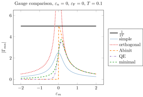
Figure 2. Comparison of gauge choices for $\delta V_{mn}=1$. Except the orthogonal gauges, all contributions $\Gamma_{mn}$ are bounded by $\frac{1}{2T}$.

3.3. Computation of unoccupied-occupied contributions employing a Schur complement

Since the $\phi_{m}$ for $m>N$ are not exactly known, a different approach is needed for obtaining the contribution $\delta\phi_{n}^{Q}$. Usually one resorts to solving the Sternheimer equation

$$\forall\ 1\leqslant n\leqslant N,\quad Q(H_{\rho}-\varepsilon_{n})Q\delta\phi_{n}^{Q}=-Q\delta V\phi_{n}\eqqcolon b_{n}$$ (45)

using iterative schemes restricted to ${\rm Ran}(Q)$. However, for $n=N$ the difference $\varepsilon_{N+1}-\varepsilon_{N}$ can become small, which deteriorates conditioning and increases the number of iterations required for convergence.

We overcome this issue by making use of the ${N_{\rm ex}}$ extra bands, which are anyway available after the SCF algorithm has completed. Following Section 2.3 the ${N_{\rm ex}}$ extra bands can be divided into two categories:

1. Some (usually the lower-energy ones) have been discarded during the response calculation because they have a too small occupation. Up to the eigensolver tolerance these are exact eigenvectors.

2. The remaining ones have served to accelerate the successive diagonalization steps during the SCF. These have not yet been fully converged.

In any case these extra bands thus offer (at least) approximate information about some $\phi_{m}$ for $m>N$, which is the underlying reason why the following approach accelerates the computation of $\delta\phi_{n}^{Q}$.

For the sake of clarity, we place ourselves here in the discrete setting: $H_{\rho}\in{\mathbb{C}}^{{N_{\rm b}}\times{N_{\rm b}}}$, $\Phi\in{\mathbb{C}}^{{N_{\rm b}}\times N}$ and $\widetilde{\Phi}\leavevmode\nobreak\ \in\leavevmode\nobreak\ {\mathbb{C}}^{{N_{\rm b}}\times{N_{\rm ex}}}$. We assume that the number of computed bands $N+{N_{\rm ex}}$ is larger than the number of occupied states $N$ and that we trust $\Phi=(\phi_{1},\dots,\phi_{N})$ but not $\widetilde{\Phi}=(\widetilde{\phi}_{N+1},\dots,\widetilde{\phi}_{N+{N_{\rm ex}}})$ to be eigenvectors. These ${N_{\rm ex}}$ extra bands consist of both contributions (1) and (2) described at the beginning of this section. We assume in addition that $(\Phi,\widetilde{\Phi})$ forms an orthonormal family and that $\widetilde{\Phi}^{*}H_{\rho}\widetilde{\Phi}$ is a diagonal matrix whose elements, denoted by $(\widetilde{\varepsilon}_{n})_{n=N+1,\dots,N+{N_{\rm ex}}}$, are not necessarily all exact eigenvalues. Note that Rayleigh-Ritz based iterative methods such as the LOBPCG algorithm fit exactly in this framework.

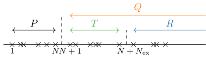
Figure 3. Graphical representation of the Schur decomposition to solve the Sternheimer equation. $P$ is the orthogonal projector onto the occupied states. $Q$ is the orthogonal projector onto the unoccupied states, and we decompose it as the sum of $T$ (extra states which we can use) and $R$ (remaining states).

We decompose

$${\rm Ran}(Q)={\rm Ran}(T)\oplus{\rm Ran}(R),$$ (46)

where $T$ is the orthogonal projector onto ${\rm Span}(\widetilde{\phi}_{m})_{N<m\leqslant N+{N_{\rm ex}}}$ and $R=Q-T$ is the projector onto the remaining (uncomputed) states, see Figure 3. Then, as $\delta\phi_{n}^{Q}\in{\rm Ran}(Q)$, we can decompose

$$\delta\phi_{n}^{Q}={\widetilde{\Phi}}\alpha_{n}+\delta\phi_{n}^{R},$$ (47)

where $\alpha_{n}\in{\mathbb{C}}^{{N_{\rm ex}}}$ and $\delta\phi_{n}^{R}\in{\rm Ran}(R)$. Plugging this into (45) we get

$$Q(H_{\rho}-\varepsilon_{n}){\widetilde{\Phi}}\alpha_{n}+Q(H_{\rho}-\varepsilon_{n})\delta\phi_{n}^{R}=b_{n}.$$ (48)

Using a Schur complement we deduce

$$\alpha_{n}=\mathopen{}\mathclose{{}\left({\widetilde{\Phi}}^{*}(H_{\rho}-\varepsilon_{n}){\widetilde{\Phi}}}\right)^{-1}\mathopen{}\mathclose{{}\left({\widetilde{\Phi}}^{*}b_{n}-{\widetilde{\Phi}}^{*}(H_{\rho}-\varepsilon_{n})\delta\phi_{n}^{R}}\right).$$ (49)

Inserting (49) into (48) and projecting on ${\rm Ran}(R)$ yields an equation in $\delta\phi_{n}^{R}$:

$$\begin{split}R(H_{\rho}-\varepsilon_{n})\mathopen{}\mathclose{{}\left[1-{\widetilde{\Phi}}\mathopen{}\mathclose{{}\left({\widetilde{\Phi}}^{*}(H_{\rho}-\varepsilon_{n}){\widetilde{\Phi}}}\right)^{-1}{\widetilde{\Phi}}^{*}(H_{\rho}-\varepsilon_{n})}\right]R\delta\phi_{n}^{R}\\ =Rb_{n}-R(H_{\rho}-\varepsilon_{n}){\widetilde{\Phi}}\mathopen{}\mathclose{{}\left({\widetilde{\Phi}}^{*}(H_{\rho}-\varepsilon_{n}){\widetilde{\Phi}}}\right)^{-1}{\widetilde{\Phi}}^{*}b_{n}.\end{split}$$ (50)

This equation can then be solved for $\delta\phi_{n}^{R}$ with a Conjugate Gradient (CG) method which is enforced to stay in ${\rm Ran}(R)$ at each iteration. Afterwards we compute $\alpha_{n}$ from (49), which yields $\delta\phi_{n}^{Q}$ from (47). This scheme has been implemented as the default solver for the Sternheimer equation in DFTK.

4. Numerical tests

For all the numerical tests, we use the DFTK software [25], a recent plane-wave DFT package in Julia. All the codes to run the simulation of this paper are available online. The Brillouin zone is discretized using a uniform Monkhorst-Pack grid [36]. We use the PBE exchange-correlation functional [39] and GTH pseudopotentials [13, 20]. The other parameters of the calculation will be specified for each example. In all the tests, we generate a perturbation $\delta V$ from atomic displacements, with local and nonlocal contributions. Then, we perform two response calculations: one with the standard approach to solve directly the Sternheimer equation (45) to compute $\delta\phi_{n}^{Q}$, the other with the (new) Schur complement approach (50). Both linear systems are solved using the conjugate gradient (CG) algorithm, with kinetic energy preconditioning (the linear solver is preconditioned with the inverse Laplacian, which is diagonal in Fourier representation), and we compare the number of iterations required to converge the norm of the residual below $10^{-9}$. Note that the Sternheimer equation is solved for all $N$ occupied orbitals and for each $k$-point.

If $T>0$ the contribution $\delta\phi_{n}^{P}$ is nonzero and has been computed using the sum-over-states formula with the minimal gauge choice (43). In terms of runtime we expect only negligible differences between the gauge choices. Moreover, since the time for this contribution is much smaller compared to the time required to solve the Sternheimer equation, we do not report a detailed performance comparison on this step in the following.

Note that our purpose in this paper is only to improve the numerical algorithms used in response computations. Although the parameters used here (exchange-correlation functionals, pseudopotentials, smearing and Brillouin zone sampling parameters, cut-off energies) might not represent physical reality appropriately, they are representative of practical calculations.

4.1. Insulators and semiconductors

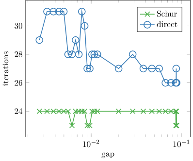
Figure 4. Number of iterations of the linear solver for the Sternheimer equation for $n=N=4$ vs the gap, with and without the Schur complement (50).

For insulators and semiconductors the gap between occupied and virtual states is usually large. One would therefore not expect a large gain from using the Schur complement (50) when computing $\delta\phi_{n}=\delta\phi_{n}^{Q}$. However, for distorted semiconductor structures or semiconductors with defects the gap can be made arbitrarily small, such that one would expect to see the Schur-complement approach to be in the advantage. We test this using an FCC Silicon crystal for which we increase the lattice constant from 10 bohrs to $11.4$ bohrs to artificially decrease and eventually close the gap. All calculations have been performed using a cut-off energy of $E_{\rm cut}=50$ Ha and a single ${k}$-point (the $\Gamma$-point). In Figure 4 we plot the number of iterations required for the linear solver of the Sternheimer equation to converge, for $n=N=4$. Using the Schur complement the number of iterations stays almost constant even when the gap decreases. In contrast, with a direct approach, the linear solver requires about $30\%$ more iterations near the closing gap.

4.2. Metals

The real advantage of using the Schur complement (50) instead of directly solving the Sternheimer equation (45) becomes apparent when computing response properties for metals at finite temperature. We use a standard heuristic which suggests to fully converge 20% more bands than the number of electrons pairs of the system, with 3 additional extra bands that are not converged by the successive eigensolvers of the SCF. We then select the “occupied” orbitals with an occupation threshold of $10^{-8}$. In addition to the number of iterations, we also compare the cost of the response calculations with and without the Schur complement (50). For this we consider the total number of Hamiltonian applications which was required to compute the response $\delta\rho$. For the small to medium-sized systems we consider here, the Hamiltonian-vector-product is the most expensive step in an DFT calculation and thus provides a representative cost indicator. Notice that both the implementation of the Schur complement and the direct method require exactly one Hamiltonian application per iteration of the CG. Additionally the Schur approach requires the computation of $H_{\rho}\widetilde{\phi}$, which is only a negligible additional cost as this is only needed once per $k$-point.

4.2.1. Aluminium

We start by considering an elongated aluminium supercell with 40 atoms. We use a cut-off energy $E_{\rm cut}=40$ Ha, a temperature $T=10^{-3}$ Ha with Fermi-Dirac smearing and a $3\times 3\times 1$ discretization of the Brillouin zone. To ensure convergence of the SCF iterations we employ the Kerker preconditioner [28]. Since the system has $120$ electrons per unit cell our usual heuristic converges 72 bands up to the tolerance of the eigensolver accompanied by 3 bands, which are not fully converged.

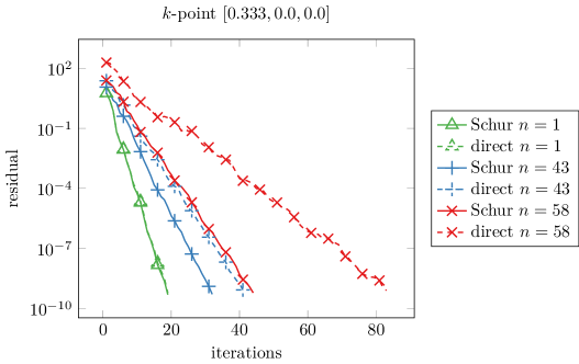
Figure 5. Convergence of the Sternheimer solver for three different orbitals for Al40. Each curve represents the convergence of the CG which solves the Sternheimer equation for one orbital: those with the slowest convergence are associated to the occupied orbitals with the highest energy.

$k$-point – coordinate	$1-[0,0,0]$	$2-[1/3,0,0]$	$5-[1/3,1/3,0]$
$N$	$69$	$58$	$67$
$\varepsilon_{N+1}-\varepsilon_{N}$	$0.0320$	$0.0134$	$0.0217$
#iterations $n=N$ Schur	$48$	$\bm{44}$	$41$
#iterations $n=N$ direct	$56$	$\bm{83}$	$58$

Table 1. Convergence data for $k$-points 1, 2 and 5 for Al40. Other $k$-points are not displayed but they all behave as one of these by symmetry. $N$ is the number of occupied bands, for an occupation threshold of $10^{-8}$.

The convergence behaviour when solving the Sternheimer equation for $k$-points of particular interest is shown in Table 1 and Figure 5. As expected, for $k$-points with a small difference $\varepsilon_{N+1}-\varepsilon_{N}$, the Schur complement (50) brings a noteworthy improvement with roughly $50\%$ fewer iterations required to achieve convergence. Since the system we consider here has numerous occupied bands — between $60$ and $70$ depending on the $k$-point — most bands already feature a well-conditioned Sternheimer equation. Considering the cost for computing the total response, the Schur approach therefore overall only achieves a reduction by 17% in the number of Hamiltonian applications, from about $17,800$ (direct) to $14,800$ (with Schur). However, it should be noted that this improvement essentially comes for free as the extra bands are anyway provided by the SCF computation as a byproduct.

4.2.2. Heusler system

Next we study the response calculation of Heusler-type transition-metal alloys. We focus mainly on the Fe2MnAl system but other compounds, such as the Fe2CrGa and CoFeMnGa alloy systems, have been tested and similar results were obtained. Heusler alloys are of considerable practical interest due to their rich and unusual magnetic and electronic properties. For instance, Fe2MnAl shows halfmetallic behaviour: the majority spin channel (denoted by $\uparrow$) behaves like a metal whereas the minority spin channel (denoted by $\downarrow$) behaves like an insulator as it has a vanishing density of states at the Fermi level. See [23], and reference therein, for more details as well as an analysis of the SCF convergence on such systems. For these systems we use a cut-off $E_{\rm cut}=45$ Ha, a temperature $T=10^{-2}$ Ha with Gaussian smearing and a $13\times 13\times 13$ discretization of the Brillouin zone. The SCF was converged using a Kerker preconditioner [28]. Moreover, as we deal with a spin-polarized system, the numerical simulation slightly differs. The orbitals $\phi_{(n,\bm{k})}^{\sigma}$ and the occupation numbers $f_{(n,\bm{k})}^{\sigma}$ depend on the spin orientation $\sigma\in\{\uparrow,\downarrow\}$ and the $f_{(n,\bm{k})}^{\sigma}$’s belong to $[0,1)$ instead of $[0,2)$. Furthermore we modify the heuristic to determine the number of bands to be computed: Fe2MnAl has ${N_{\rm el}}=50$ electrons per unit cell and we use $25+0.2\times 50=35$ fully converged bands per $k$-point, complemented by 3 additional bands, which are not checked for convergence.

spin channel	$\uparrow$	$\downarrow$
$N$	$28$	$26$
$\varepsilon_{N+1}-\varepsilon_{N}$	$0.0423$	$0.0154$
#iterations $n=N$ Schur	$\bm{45}$	$\bm{45}$
#iterations $n=N$ direct	$\bm{86}$	$\bm{103}$

Table 2. Convergence data for the two spin channels of the $k$-point with reduced coordinates $[0.385,0.231,0.077]$ for Fe2MnAl. $N$ is the number of occupied bands, for an occupation threshold of $10^{-8}$.

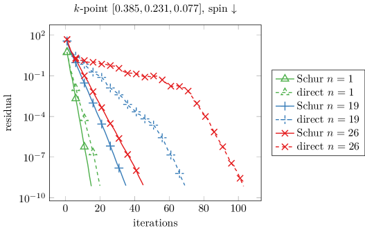
Figure 6. Convergence of the Sternheimer solver for three different orbitals for Fe2MnAl. Each curve represents the convergence of the CG which solves the Sternheimer equation for one orbital: those with the slowest convergence are associated to the occupied orbitals with the highest energy.

We show in Table 2 and Figure 6 the results for the two spin channels of the $k$-point with reduced coordinates $[0.385,0.231,0.077]$. The other $k$-points behave similarly. Since both channels feature a small difference $\varepsilon_{N+1}-\varepsilon_{N}$ using the Schur complement (50) to solve the Sternheimer equation has a significant impact: for the orbitals with highest energy it reduces the number of iterations by half. For the direct approach we notice a plateau where the solver encounters difficulties to converge the Sternheimer equation for the $N$-th orbital due to the small gap.

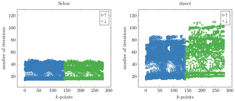
Figure 7. Histogram of the number of iterations of the CG to solve the Sternheimer equation, with and without the Schur complement (50). On the $x$-axis, the $k$-point index number: the first 140 (blue $\circ$) have spins up, and the last 140 (green $\times$) have the same coordinates but with spins down. For each of these $k$-points, we plot the number of iterations for every occupied band of the $k$-point.

Unlike the aluminium case the improvements observed for the Heusler alloys are not restricted to a small number of bands. In Figure 7 we contrast the number of iterations required to solve the Sternheimer equation for every band at every $k$-point with and without using the Schur complement. Notice that lattice symmetries allow to reduce the number of explicitly treated $k$-points to $140$ albeit we are using a $13\times 13\times 13$ $k$-point grid. In terms of the total number of Hamiltonian applications required for the response calculation, the Schur complement achieves a reduction by roughly $40\%$, from around $344,000$ (without Schur) to $208,000$ (with Schur). It should be noted that in this system the standard heuristic caused a large portion of the available extra bands to be fully converged, thus providing an ideal setting for the Schur complement approach to be effective. For example for the $k$-point discussed in Table 2 seven extra bands have been fully converged and an additional three partially. Given the enormous importance of Heusler systems and the known numerical difficulties for computing response properties in these systems, our result is encouraging and motivates the development of a more economical heuristic for choosing the number of converged bands in future work.

4.3. Comparison to shifted Sternheimer approaches

In the literature other strategies for computing $\delta\rho$ have been reported. We briefly consider the approach proposed in [1], where the response is computed as

$$\delta\rho(\bm{r})=\sum_{n=1}^{N}2\phi_{n}^{*}(\bm{r})\delta\phi_{n}(\bm{r})-f^{\prime}_{n}\delta\varepsilon_{\rm F}|\phi_{n}(\bm{r})|^{2}.$$ (51)

Instead of splitting $\delta\phi_{n}$ into two contributions, the full $\delta\phi_{n}$ is computed for all $n\leqslant N$ by solving the shifted Sternheimer equation

$$(H_{\rho}+S-\varepsilon_{n})\delta\phi_{n}=-(f_{n}-S_{n})\delta V\phi_{n}.$$ (52)

Here $S:{\rm Ran}(P)\to{\rm Ran}(P)$ is a shift operator acting on the space of occupied orbitals, chosen so that the linear system is nonsingular (for any $n\leqslant N$, $H_{\rho}-\varepsilon_{n}$ is not invertible). Then, $S_{n}$ is chosen for every $n\leqslant N$ such that $\delta\rho$ from (51) satisfies (20). However, as $S$ only acts on ${\rm Ran}(P)$, equation still becomes badly conditioned if $\varepsilon_{N+1}-\varepsilon_{N}$ is too small. This becomes apparent when solving the shifted Sternheimer equation (52) for the Fe2MnAl system, see Figure 8.

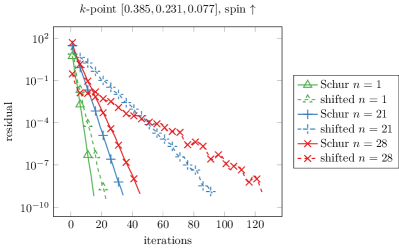
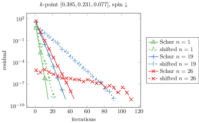
Figure 8. Resolution of the Sternheimer equation for both spin channels of one specific $k$-point for the Fe2MnAl system, with the Schur approach (50) and the shifted approach (52). Note that for this particular $k$-point, the spin $\downarrow$ channel has a starting point with already small residual for the highest occupied energy level. This is due to the term $f_{n}$ appearing in (52), and the convergence is still slow.

For the orbital responses of the highest-energy occupied bands the CG iterations on the shifted Sternheimer equation converge very slowly — in contrast to the Schur complement approach (50) we proposed in this work. In terms of the number of Hamiltonian applications, the shifted Sternheimer strategy required around $492,000$ applications versus $208,000$ for the Schur complement approach.

5. Conclusion

In density-functional theory the simulation of many physical properties requires the computation of the response of the ground-state density to an external perturbation. In this work we have reviewed the standard formalism of such response calculations from the point of view of numerical analysis. We provided an overview of the possible gauge choices for representing the density response, summarizing and contrasting the approaches employed by state-of-the-art codes such as Quantum Espresso [12] or Abinit [41] in a common framework.

Based on our analysis we furthermore suggested two novel approaches for DFT response calculations. For the occupied-occupied part of the response we developed a gauge choice based on the idea to maximize numerical stability in the involved sums by minimizing the numerical range of the individual orbital contributions. For the occupied-unoccupied part of the response we suggested a novel approach to solving the Sternheimer equation based on a Schur complement. Key idea of this approach is to make use of the additional (partially) converged bands, which are available as a byproduct from the preceding self-consistent field (SCF) procedure (which yields the ground-state density). Without additional computational effort this allows to improve the conditioning of the Sternheimer equation and thus accelerate its convergence. We demonstrated this numerically on a number of practically relevant problems, including response calculations on small-gapped semiconductors, elongated metallic slabs or numerically challenging Heusler alloy systems. Overall the Schur complement approach allowed to obtain a converged response saving up to 40% in the required Hamiltonian applications — the cost-dominating step in small to medium-sized DFT problems. For larger systems we similarly expect savings from introducing a Schur complement technique, even though algorithms commonly employ different trade-offs.

In this work we followed standard heuristics for selecting the number of extra bands to employ in the SCF calculations and thus the number of additional bands available when solving the response problem. However, our results emphasize the need for a more robust understanding between the computed number of bands and the observed rate of convergence. We have provided some initial ideas for such an analysis in the appendix, but leave a more exhaustive discussion for future work.

Appendix A Choosing the number of extra bands

In this paper, we saw through various numerical examples that using a Schur complement to compute the unoccupied-occupied contributions to the orbitals’ response improves the convergence of the Sternheimer equation. In this appendix, we quantify this acceleration and discuss how this idea can be used to select the number of bands to be computed. Considering the straight convergence curves from Figures 5–6 suggest that the convergence of the CG is indeed led by the square root of the condition number of the system matrix (see [43, Section 9]) when using the Schur complement. Key idea will thus be to estimate the condition number of the linear system (50).

A.1. Numerical analysis

To analyse the condition number of the Schur complement, we consider the following specific setting

$$\begin{cases}H_{\rho}\phi_{n}=\varepsilon_{n}\phi_{n},\quad\varepsilon_{1}\leqslant\varepsilon_{2}\leqslant\cdots\\ \mathopen{}\mathclose{{}\left\langle\phi_{n},\phi_{m}}\right\rangle=\delta_{nm},\end{cases}$$ (53)

where $H_{\rho}\in{\mathbb{C}}^{{N_{\rm b}}\times{N_{\rm b}}}$ is typically the discretized self-consistent Hamiltonian of the system, at some $k$-point. We assume that we have $N$ occupied orbitals that have an occupation number higher than the threshold we fixed and that we have ${N_{\rm ex}}$ extra bands, as explained in Section 3.3. In summary, we have at our disposal $N+{N_{\rm ex}}$ bands in total: $\Phi=(\phi_{1},\dots,\phi_{N})$ are occupied, fully converged bands and the extra bands $\Phi_{\rm ex}^{\ell}=(\phi^{\ell}_{N+1},\dots,\phi^{\ell}_{N+{N_{\rm ex}}})$ are not necessarily all converged. We added here the exponent $\ell$ as we make the following assumptions:

• for any $\ell\in{\mathbb{N}}$, $(\Phi,\Phi_{\rm ex}^{\ell})$ is an orthonormal family;

• for any $\ell\in{\mathbb{N}}$, $(\Phi_{\rm ex}^{\ell})^{*}H_{\rho}\Phi_{\rm ex}^{\ell}\in{\mathbb{C}}^{{N_{\rm ex}}\times{N_{\rm ex}}}$ is a diagonal matrix whose elements are labelled $\varepsilon_{m}^{\ell}\coloneqq\mathopen{}\mathclose{{}\left\langle\phi_{m}^{\ell},H_{\rho}\phi_{m}^{\ell}}\right\rangle$ for $N+1\leqslant m\leqslant N+{N_{\rm ex}}$;

• as $\ell\to+\infty$, $(\phi^{\ell}_{m},\varepsilon^{\ell}_{m})\to(\phi_{m},\varepsilon_{m})$.

All these assumptions are satisfied for instance if the sequence $(\Phi,\Phi_{\rm ex}^{\ell})_{l\in{\mathbb{N}}}$ is generated by any Rayleigh-Ritz based eigensolver (for instance the LOBPCG eigensolver [31]), which is the case by default in DFTK. For every $\ell$, we can thus decompose the plane-wave approximation space ${\mathcal{H}}=X_{{N_{\rm b}}}$ (with ${N_{\rm b}}\gg N+{N_{\rm ex}}$) in two different ways:

$${\mathcal{H}}={\rm Ran}(P)\oplus{\rm Ran}(T)\oplus{\rm Ran}(R)\quad\text{and}\quad{\mathcal{H}}={\rm Ran}(P)\oplus{\rm Ran}(T^{\ell})\oplus{\rm Ran}(R^{\ell}),$$ (54)

where

$$P\coloneqq\sum_{n=1}^{N}\phi_{n}\phi_{n}^{*}\quad\text{and}\quad\begin{cases}T\coloneqq\sum_{n=N+1}^{{N_{\rm ex}}}\phi_{n}\phi_{n}^{*},\quad R\coloneqq 1-P-T\\ T^{\ell}\coloneqq\sum_{n=N+1}^{{N_{\rm ex}}}\phi_{n}^{\ell}(\phi_{n}^{\ell})^{*},\quad R^{\ell}\coloneqq 1-P-T^{\ell},\end{cases}$$ (55)

are all orthogonal projectors. In these two decompositions, $H_{\rho}$ has the associated block representations:

$$H_{\rho}=\begin{pmatrix}E&0&0\\ 0&E_{\rm ex}&0\\ 0&0&\ddots\end{pmatrix}\quad\text{and}\quad H_{\rho}=\begin{pmatrix}E&0&0\\ 0&E^{\ell}_{\rm ex}&R^{\ell}H_{\rho}T^{\ell}\\ 0&T^{\ell}H_{\rho}R^{\ell}&R^{\ell}H_{\rho}R^{\ell}\end{pmatrix}$$ (56)

where $E\coloneqq{\rm Diag}(\varepsilon_{1},\dots,\varepsilon_{n})$, $E_{\rm ex}\coloneqq{\rm Diag}(\varepsilon_{N+1},\dots,\varepsilon_{N+{N_{\rm ex}}})$ and $E_{\rm ex}^{\ell}\coloneqq{\rm Diag}(\varepsilon^{\ell}_{N+1},\dots,\varepsilon^{\ell}_{N+{N_{\rm ex}}})$ are diagonal matrices. Moreover, note that as $\Phi^{\ell}_{\rm ex}\to\Phi_{\rm ex}$, the residuals $R^{\ell}H_{\rho}T^{\ell}$ converge to $0$.

Now, we fix $n\leqslant N$ and we compute the condition number of the linear system (50). Enforcing the CG to stay at each iteration in ${\rm Ran}(R^{\ell})$, this condition number is given by the ratio of the largest and smallest nonzero eigenvalues of

$$H_{n}^{\ell}+X_{n}^{\ell},$$ (57)

where

$$\begin{split}H_{n}^{\ell}\coloneqq R^{\ell}(H_{\rho}-\varepsilon_{n})R^{\ell}\quad\text{and}\quad X_{n}^{\ell}&=-R^{\ell}(H_{\rho}-\varepsilon_{n})\Phi_{\rm ex}^{\ell}(E_{\rm ex}^{\ell}-\varepsilon_{n})^{-1}(\Phi_{\rm ex}^{\ell})^{*}(H_{\rho}-\varepsilon_{n})R^{\ell}\\ &=-R^{\ell}H_{\rho}\Phi_{\rm ex}^{\ell}(E_{\rm ex}^{\ell}-\varepsilon_{n})^{-1}(\Phi_{\rm ex}^{\ell})^{*}H_{\rho}R^{\ell}.\end{split}$$ (58)

Here $E^{\ell}_{\rm ex}-\varepsilon_{n}$ is diagonal and thus explicitly invertible if $\ell$ is large enough as $\varepsilon_{N+1}^{\ell}\to\varepsilon_{N+1}>\varepsilon_{N}\geqslant\varepsilon_{n}$. We focus for the moment on the smallest nonzero eigenvalue, that is $\varepsilon^{\ell}_{N+{N_{\rm ex}}+1}-\varepsilon_{n}$. The condition number being proportional to the inverse of the smallest eigenvalue, we now derive a lower bound of $\varepsilon^{\ell}_{N+{N_{\rm ex}}+1}-\varepsilon_{n}$ in order to get an upper bound on the condition number of (57). When $\ell\to+\infty$, we have $X_{n}^{\ell}\to 0$ (as $RH_{\rho}\Phi_{\rm ex}=0$) and $H_{n}^{\ell}\to H_{n}\coloneqq R(H_{\rho}-\varepsilon_{n})R$ whose smallest nonzero eigenvalue is $\varepsilon_{N+{N_{\rm ex}}+1}-\varepsilon_{n}$. We use next a perturbative approach to effectively approximate the condition number of (57).

We use a standard eigenvalue perturbation result, whose proof is recalled for the sake of completeness. It is directly adapted from the general case of self-adjoint bounded below operators with symmetric perturbations studied for instance in [11].

Proposition 1.

Let $N\in{\mathbb{N}}$, $H_{0},W\in{\mathbb{C}}^{N\times N}$ be Hermitian matrices and $\alpha\geqslant 0$ such that $H_{0}+\alpha>0$. Then, the eigenvalues of $H\coloneqq H_{0}+W$ and $H_{0}$ satisfy

$$\mathopen{}\mathclose{{}\left|\nu_{i}(H)-\nu_{i}(H_{0})}\right|\leqslant(\nu_{i}(H_{0})+\alpha)\mathopen{}\mathclose{{}\left\|W}\right\|_{H_{0},\alpha},$$ (59)

where $\mathopen{}\mathclose{{}\left\|W}\right\|_{H_{0},\alpha}$ is the operator norm of $(H_{0}+\alpha)^{-1/2}W(H_{0}+\alpha)^{-1/2}$ and $\nu_{i}(A)$ is the $i$-th lowest eigenvalue of the matrix $A$.

Proof.

Let $u\in{\mathbb{C}}^{N}$ and define $v\coloneqq(H_{0}+\alpha)^{1/2}u$. Then,

$$\begin{split}\mathopen{}\mathclose{{}\left|\mathopen{}\mathclose{{}\left\langle u,Hu}\right\rangle-\mathopen{}\mathclose{{}\left\langle u,H_{0}u}\right\rangle}\right|=\mathopen{}\mathclose{{}\left|\mathopen{}\mathclose{{}\left\langle u,Wu}\right\rangle}\right|&=\mathopen{}\mathclose{{}\left|\mathopen{}\mathclose{{}\left\langle v,(H_{0}+\alpha)^{-1/2}W(H_{0}+\alpha)^{-1/2}v}\right\rangle}\right|\\ &\leqslant\mathopen{}\mathclose{{}\left\|W}\right\|_{H_{0},\alpha}\mathopen{}\mathclose{{}\left\langle v,v}\right\rangle=\mathopen{}\mathclose{{}\left\|W}\right\|_{H_{0},\alpha}\mathopen{}\mathclose{{}\left\langle u,(H_{0}+\alpha)u}\right\rangle.\end{split}$$ (60)

Therefore,

$$(1-\mathopen{}\mathclose{{}\left\|W}\right\|_{H_{0},\alpha})\mathopen{}\mathclose{{}\left\langle u,H_{0}u}\right\rangle-\alpha\mathopen{}\mathclose{{}\left\|W}\right\|_{H_{0},\alpha}\mathopen{}\mathclose{{}\left\langle u,u}\right\rangle\leqslant\mathopen{}\mathclose{{}\left\langle u,Hu}\right\rangle\leqslant(1+\mathopen{}\mathclose{{}\left\|W}\right\|_{H_{0},\alpha})\mathopen{}\mathclose{{}\left\langle u,H_{0}u}\right\rangle+\alpha\mathopen{}\mathclose{{}\left\|W}\right\|_{H_{0},\alpha}\mathopen{}\mathclose{{}\left\langle u,u}\right\rangle.$$ (61)

The min-max theorem then yields for $i=1,\dots,N$,

$$(1-\mathopen{}\mathclose{{}\left\|W}\right\|_{H_{0},\alpha})\nu_{i}(H_{0})-\alpha\mathopen{}\mathclose{{}\left\|W}\right\|_{H_{0},\alpha}\leqslant\nu_{i}(H)\leqslant(1+\mathopen{}\mathclose{{}\left\|W}\right\|_{H_{0},\alpha})\nu_{i}(H_{0})+\alpha\mathopen{}\mathclose{{}\left\|W}\right\|_{H_{0},\alpha},$$ (62)

which gives the desired inequality. ∎

In our case, we can apply this result to

$$H_{n}^{\ell}+X_{n}^{\ell}=H_{n}+(H_{n}^{\ell}-H_{n})+X_{n}^{\ell},$$ (63)

with $H_{0}=H_{n}$, $W=W_{n}^{\ell}\coloneqq(H_{n}^{\ell}-H_{n})+X_{n}^{\ell}$ and $\alpha=\varepsilon_{N+{N_{\rm ex}}+1}-\varepsilon_{n}>0$. Proposition 1 applied to the $(N+{N_{\rm ex}}+1)$-th eigenvalues then yields

$$\varepsilon_{N+{N_{\rm ex}}+1}^{\ell}-\varepsilon_{n}\geqslant\mathopen{}\mathclose{{}\left(\varepsilon_{N+{N_{\rm ex}}+1}-\varepsilon_{n}}\right)\mathopen{}\mathclose{{}\left(1-2\mathopen{}\mathclose{{}\left\|W_{n}^{\ell}}\right\|_{H_{n},\varepsilon_{N+{N_{\rm ex}}+1}-\varepsilon_{n}}}\right)\approx\mathopen{}\mathclose{{}\left(\varepsilon_{N+{N_{\rm ex}}+1}-\varepsilon_{n}}\right),$$ (64)

where we assume that $2\mathopen{}\mathclose{{}\left\|W_{n}^{\ell}}\right\|_{H_{n},\varepsilon_{N+{N_{\rm ex}}+1}-\varepsilon_{n}}$ is small enough to be negligible with respect to 1, which is the case if the extra states are sufficiently converged. Now, if this bound is valid in theory, in practice we do not have access to $\varepsilon_{N+{N_{\rm ex}}+1}$ as we work with $N+{N_{\rm ex}}$ bands only. However, up to loosing sharpness, we can use that $\varepsilon_{N+{N_{\rm ex}}+1}\geqslant\varepsilon_{N+{N_{\rm ex}}}$ where $\varepsilon_{N+{N_{\rm ex}}}$ can be estimated using the last extra band. Indeed, using for instance the Bauer-Fike bound ([24, Theorem 1] or [42]), we obtain

$$\varepsilon_{N+{N_{\rm ex}}}\geqslant\varepsilon_{N+{N_{\rm ex}}}^{\ell}-\mathopen{}\mathclose{{}\left\|r_{N+{N_{\rm ex}}}^{\ell}}\right\|,$$ (65)

where $r_{N+{N_{\rm ex}}}^{\ell}$ is the residual associated to the last extra band. Of course, this estimate is not sharp as we expect the error on the eigenvalue to behave as the square of the residual, but this requires to estimate the gap to the rest of the spectrum, see for instance the Kato-Temple bound [24, Theorem 2]. In the end, we have the following lower bound for $\varepsilon_{N+{N_{\rm ex}}+1}^{\ell}-\varepsilon_{n}$:

$$\varepsilon_{N+{N_{\rm ex}}+1}^{\ell}-\varepsilon_{n}\geqslant\mathopen{}\mathclose{{}\left(\varepsilon_{N+{N_{\rm ex}}}^{\ell}-\varepsilon_{n}-\mathopen{}\mathclose{{}\left\|r_{N+{N_{\rm ex}}}^{\ell}}\right\|}\right)\approx\varepsilon_{N+{N_{\rm ex}}}^{\ell}-\varepsilon_{n},$$ (66)

where we assume again that $\mathopen{}\mathclose{{}\left\|r_{N+{N_{\rm ex}}}^{\ell}}\right\|$ is small enough with respect to $\varepsilon_{N+{N_{\rm ex}}}^{\ell}-\varepsilon_{n}$.

We can now derive an upper bound on $\kappa_{n}^{\ell}$, the condition number of (57). It is given by the ratio of its highest eigenvalue and $\varepsilon_{N+{N_{\rm ex}}+1}^{\ell}-\varepsilon_{n}$. Since the Laplace operator is the higher-order term in the Kohn-Sham Hamiltonian, the highest eigenvalue is, as usually in plane-wave simulations, of order $E_{\rm cut}$. With proper kinetic preconditioning, we can assume that its contribution to the condition number of the linear system is constant with respect to $E_{\rm cut}$ and $n$ so that, finally,

$$\kappa_{n}^{\ell}\lesssim\frac{C}{\varepsilon_{N+{N_{\rm ex}}+1}^{\ell}-\varepsilon_{n}}\lesssim\frac{C}{\varepsilon_{N+{N_{\rm ex}}}^{\ell}-\varepsilon_{n}}.$$ (67)

Therefore the condition number is bounded from above by $C/(\varepsilon_{N+{N_{\rm ex}}}^{\ell}-\varepsilon_{n})$ to first-order. The number of CG iterations to solve the linear system (50) with a given accuracy is then proportional to the square root of the condition number of the matrix (57) (see [43]):

$$\sqrt{\kappa_{n}^{\ell}}\lesssim\sqrt{\frac{C}{{\varepsilon_{N+{N_{\rm ex}}}^{\ell}-\varepsilon_{n}}}}.$$ (68)

Note that this upper bound is valid provided that the extra bands are converged enough, not necessarily fully, and proper kinetic preconditioning is employed.

Estimate (68) leads, as expected, to the qualitative conclusion that the more extra bands we use, the higher the difference $\varepsilon_{N+{N_{\rm ex}}}^{\ell}-\varepsilon_{n}$ and the faster the convergence. However, note that it is not possible to evaluate directly the convergence speed as the constant $C$ is a priori unknown, in particular if we use preconditioners.

A.2. An adaptive strategy to choose the number of extra bands

The main bottleneck of (68) is the estimation of the constant $C$. However, one can reasonably assume that this constant does not depend too much on $n$, so that the ratio between the number of iterations to reach convergence between the last occupied band ($n=N$) and the first band $(n=1)$ can be estimated by

$$\xi_{{N_{\rm ex}}}^{\ell}\coloneqq\sqrt{\frac{\varepsilon_{N+{N_{\rm ex}}}^{\ell}-\varepsilon_{1}}{\varepsilon_{N+{N_{\rm ex}}}^{\ell}-\varepsilon_{N}}},$$ (69)

This ratio can be of interest as (68) suggests that the Sternheimer solver converges the fastest for $n=1$ and the slowest for $n=N$.

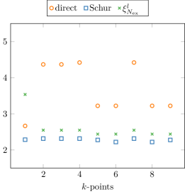
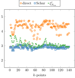
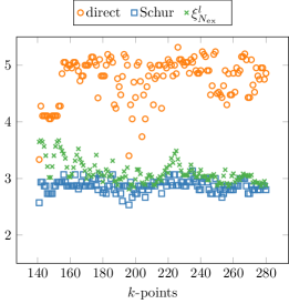
Figure 9. Comparison between the ratio $\xi_{{N_{\rm ex}}}^{\ell}$ ($\times$) and the ratios of the experimental number of iterations between the first and last occupied bands, with ($\square$) and without ($\circ$) the Schur complement (50). On the $x$-axis is the index of the $k$-point. [Left] Al40 [Middle] Fe2MnAl spin up channels [Right] Fe2MnAl spin down channels.

We plot in Figure 9 the upper bound $\xi_{{N_{\rm ex}}}^{\ell}$ as well as the computed ratios between the number of iterations of the first and last bands for the systems we considered in Section 4. These plots show that $\xi_{{N_{\rm ex}}}^{\ell}$ is indeed an upper bound of the actual ratio. This bound does not seem to be sharp however. This is due to the successive approximations we made to obtain this estimate. Plots in Figure 9 also confirm that if, for every $k$-point, the ratio of the number of iterations between the first and last occupied bands is assumed to be an accurate indicator of the efficiency of the Sternheimer solver, then using the Schur complement (50) always make this ratio smaller.

If we want the ratio of the number of iterations between the first and the last occupied bands to be lower than some target ratio $\xi_{T}$ (for instance 3), Figure 9 suggests that the computable ratio $\xi_{{N_{\rm ex}}}^{\ell}$ can help in choosing the number of extra bands to reach this target ratio. We propose in Algorithm 1 an adaptive algorithm to select the number of extra bands as a post-processing step after termination of the SCF. The basic idea is that, given the initial output $(\Phi,\Phi_{\rm ex}^{\ell})$ with $\ell=0$ of an SCF calculation, one iterates $\Phi_{\rm ex}^{\ell}\to\Phi_{\rm ex}^{\ell+1}$ where $\Phi_{\rm ex}^{\ell}$ gathers the extra bands. At each iteration $\ell$, we compute $\xi_{{N_{\rm ex}}}^{\ell}$ and check if it is below the target ratio. If not, we compute more approximated eigenvectors, that we converge until the residual $\mathopen{}\mathclose{{}\left\|r_{N+{N_{\rm ex}}}^{\ell}}\right\|$ is negligible with respect to $\varepsilon_{N+{N_{\rm ex}}}^{\ell}-\varepsilon_{N}$, and so on. To generate such a residual, after adding a random extra band properly orthonormalized, we update the extra bands using a LOBPCG with tolerance

$${\rm tol}=(\varepsilon_{N+{N_{\rm ex}}-1}^{\ell}-\varepsilon_{N})/50.$$ (70)

Note that we use $\varepsilon_{N+{N_{\rm ex}}-1}^{\ell}$ instead of $\varepsilon_{N+{N_{\rm ex}}}^{\ell}$: this is done for the sake of simplicity, instead of updating the tolerance on the fly with $\varepsilon_{N+{N_{\rm ex}}}^{\ell}$ changing at each iteration of the LOBPCG.

Data: target ratio $\xi_{T}$, ${N_{\rm ex}}$, $\ell$, $\xi_{{N_{\rm ex}}}^{\ell}$

while $\xi_{{N_{\rm ex}}}^{\ell}>\xi_{T}$  do

       add random extra band $\phi_{\rm new}$ in the orthogonal of ${\rm Span}(\Phi,\Phi_{\rm ex}^{\ell})$;

       ${N_{\rm ex}}\leftarrow{N_{\rm ex}}+1$;

       update on the fly the extra bands with tolerance from (70) using the LOBPCG method;

       $\Phi_{\rm ex}^{\ell+1}\leftarrow(\Phi_{\rm ex}^{\ell},\phi_{\rm new})$ and $E_{\rm ex}^{\ell+1}\leftarrow(\Phi_{\rm ex}^{\ell+1})^{*}H_{\rho}\Phi_{\rm ex}^{\ell+1}$;

       $\ell\leftarrow\ell+1$;

       compute $\xi_{{N_{\rm ex}}}^{\ell}$ with (69);

end while

Algorithm 1 Adaptive choice of the number of extra bands

A.3. Numerical tests

We test this strategy on the systems investigated in Section 4, with different values for the target ratio $\xi_{T}$ in order to see a noticeable improvement for each system. In practice, we suggest this ratio to be between 2 and 3.

We first start with the Al40 system. Figure 9 [Left] suggests that the default choice of extra bands already gives satisfying results by reaching a ratio of approximately 2.5 for all $k$-points but the $\Gamma$-point (for which there is no real issue with the Sternheimer equation, according to Table 1). We thus run Algorithm 1 with a smaller target ratio $\xi_{T}=2.2$. We use as initial value for ${N_{\rm ex}}$ the default value for each $k$-point. Results are plotted in Section A.3 [Left] and suggests adding 15 extra bands. Running again the simulations from Section 4 with 72 fully converged bands and 18 additional, not fully converged, bands yields indeed an improvement in the convergence of the CG when solving the Sternheimer equation with the Schur complement method. Moreover, in Figure 10, the ratio $\xi_{{N_{\rm ex}}}^{\ell}$ indeed lies below the target ratio $\xi_{T}=2.2$, and matches this ratio for the $k$-points that caused difficulties for the Sternheimer equation solver to converge. In terms of computational time, the number of Hamiltonian applications to compute the response has been reduced from $\sim 14,800$ with the default number of extra bands to $\sim 12,800$. However, running the algorithm required $\sim 3,400$ additional Hamiltonian applications, making the total amount of Hamiltonian applications higher than that of the Schur approach with the standard heuristic.

Al40, $\xi_{T}=2.2$

Fe2MnAl, $\xi_{T}=2.5$

& $k$-point / spin $96\uparrow$ $96\downarrow$ $72\uparrow$ $72\downarrow$ $N$ $28$ $26$ $29$ $26$ $\text{default }N_{\rm ex}$ $10$ $12$ $9$ $12$ $\text{suggested }N_{\rm ex}$ $16$ $18$ $17$ $20$ #iterations $n=1$ Schur $15$ $15$ $15$ $15$ #iterations $n=N$ Schur $36$ $35$ $35$ $35$

Table 3. Suggested number of extra bands for Al40 and Fe2MnAl to reach the target ratio $\xi_{T}$, obtained with Algorithm 1 with default ${N_{\rm ex}}$ as starting point, as well as the number of iterations to reach convergence with the newly suggested ${N_{\rm ex}}$. Note that the ratio between iterations indeed lies below the target ratio $\xi_{T}$.

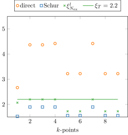
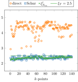
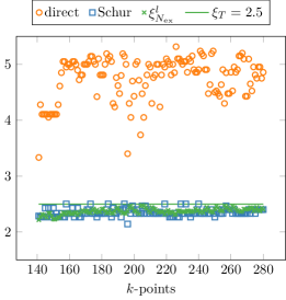
Figure 10. Comparison between the ratio $\xi_{{N_{\rm ex}}}^{\ell}$ ($\times$) and the ratios of the measured number of iterations between the first and last occupied bands, with ($\square$) and without ($\circ$) the Schur complement (50). On the $x$-axis is the index of the $k$-point. [Left] Al40 with 15 additional extra bands. [Left] Fe2MnAl spin $\uparrow$ with 8 additional bands. [Right] Fe2MnAl spin $\downarrow$ with 8 additional bands.

Similarly, for Fe2MnAl, we run Algorithm 1 with target ratio $\xi_{T}=2.5$ as well as initial value the default ${N_{\rm ex}}$ for all the 140 $k$-points and spin polarizations. We present in Section A.3 [Right] the output for both spin polarizations of two particular $k$-points. The results are similar for the rest of the $k$-points and the maximum additional extra bands suggested by the algorithm is 8. We thus run the same simulations as in Section 4 but this time with 35 fully converged bands and $11$ extra, nonnecessarily converged, bands. We indeed see for these two $k$-points that the target ratio has been reached, and that the number of iterations to converge is smaller than for the default choice we made in Table 2. In Figure 10, we plot the ratios $\xi_{{N_{\rm ex}}}^{\ell}$ as well as the actual ratios and they almost all lie below the target ratio. Contrarily to Al40, we note however that the actual measured ratios are not always below the indicator $\xi_{{N_{\rm ex}}}^{\ell}$. In terms of computational time, the number of Hamiltonian applications has been reduced from $\sim 208,000$ with the default choice of ${N_{\rm ex}}$ to $\sim 179,000$. Again, running the algorithm required $\sim 49,000$ additional Hamiltonian applications, making it more expensive than using the default number of extra bands.

It appears that Algorithm 1 can be used to choose the number of extra bands in order to reach a given ratio $\xi_{T}$. However, using the algorithm as such is not useful in practice as it requires a too high number of Hamiltonian applications, making this strategy less interesting than the Schur approach we proposed with the default choice of extra bands. Strategies to reduce the number of Hamiltonian applications in order to choose an appropriate number of extra bands will be subject of future work.

References

- [1] S. Baroni, S. de Gironcoli, A. Dal Corso, and P. Giannozzi. Phonons and related crystal properties from density-functional perturbation theory. Reviews of Modern Physics, 73(2):515–562, 2001.
- [2] S. Baroni, P. Giannozzi, and A. Testa. Green’s-function approach to linear response in solids. Physical Review Letters, 58(18):1861–1864, 1987.
- [3] E. Cancès, R. Chakir, and Y. Maday. Numerical analysis of the planewave discretization of some orbital-free and Kohn-Sham models. ESAIM: Mathematical Modelling and Numerical Analysis, 46(2):341–388, 2012.
- [4] É. Cancès, A. Deleurence, and M. Lewin. A New Approach to the Modeling of Local Defects in Crystals: The Reduced Hartree-Fock Case. Communications in Mathematical Physics, 281(1):129–177, 2008.
- [5] E. Cancès, V. Ehrlacher, D. Gontier, A. Levitt, and D. Lombardi. Numerical quadrature in the Brillouin zone for periodic Schrödinger operators. Numerische Mathematik, 144(3):479–526, 2020.
- [6] E. Cancès, G. Kemlin, and A. Levitt. Convergence analysis of direct minimization and self-consistent iterations. SIAM Journal on Matrix Analysis and Applications, 42(1):243–274, 2021.
- [7] E. Cancès, A. Levitt, Y. Maday, and C. Yang. Numerical methods for Kohn-Sham models: Discretization, algorithms, and error analysis. In E. Cancès and G. Friesecke, editors, Density Functional Theory, chapter 7. Springer, 2021.
- [8] E. Cancès and M. Lewin. The Dielectric Permittivity of Crystals in the Reduced Hartree–Fock Approximation. Archive for Rational Mechanics and Analysis, 197(1):139–177, 2010.
- [9] E. Cancès and N. Mourad. A mathematical perspective on density functional perturbation theory. Nonlinearity, 27(9):1999–2033, 2014.
- [10] I. Catto, C. L. Bris, and P. L. Lions. Mathematical Theory of Thermodynamic Limits : Thomas- Fermi Type Models. Oxford University Press, 1998.
- [11] G. Dusson, I. Sigal, and B. Stamm. Analysis of the Feshbach-Schur method for the planewave discretizations of Schrödinger operators. arXiv:2008.10871 [cs, math], 2020.
- [12] P. Giannozzi, S. Baroni, N. Bonini, M. Calandra, R. Car, C. Cavazzoni, D. Ceresoli, G. L. Chiarotti, M. Cococcioni, I. Dabo, A. Dal Corso, S. de Gironcoli, S. Fabris, G. Fratesi, R. Gebauer, U. Gerstmann, C. Gougoussis, A. Kokalj, M. Lazzeri, L. Martin-Samos, N. Marzari, F. Mauri, R. Mazzarello, S. Paolini, A. Pasquarello, L. Paulatto, C. Sbraccia, S. Scandolo, G. Sclauzero, A. P. Seitsonen, A. Smogunov, P. Umari, and R. M. Wentzcovitch. QUANTUM ESPRESSO: A modular and open-source software project for quantum simulations of materials. Journal of Physics. Condensed Matter: An Institute of Physics Journal, 21(39):395502, 2009.
- [13] S. Goedecker, M. Teter, and J. Hutter. Separable dual-space Gaussian pseudopotentials. Physical Review B, 54(3):1703, 1996.
- [14] D. Gontier and S. Lahbabi. Convergence rates of supercell calculations in the reduced Hartree-Fock model. ESAIM: Mathematical Modelling and Numerical Analysis, 50(5):1403–1424, 2016.
- [15] X. Gonze. Adiabatic density-functional perturbation theory. Physical Review A, 52(2):1096–1114, 1995.
- [16] X. Gonze. Perturbation expansion of variational principles at arbitrary order. Physical Review A, 52(2):1086–1095, 1995.
- [17] X. Gonze, B. Amadon, G. Antonius, F. Arnardi, L. Baguet, J.-M. Beuken, J. Bieder, F. Bottin, J. Bouchet, E. Bousquet, N. Brouwer, F. Bruneval, G. Brunin, T. Cavignac, J.-B. Charraud, W. Chen, M. Côté, S. Cottenier, J. Denier, G. Geneste, P. Ghosez, M. Giantomassi, Y. Gillet, O. Gingras, D. R. Hamann, G. Hautier, X. He, N. Helbig, N. Holzwarth, Y. Jia, F. Jollet, W. Lafargue-Dit-Hauret, K. Lejaeghere, M. A. L. Marques, A. Martin, C. Martins, H. P. C. Miranda, F. Naccarato, K. Persson, G. Petretto, V. Planes, Y. Pouillon, S. Prokhorenko, F. Ricci, G.-M. Rignanese, A. H. Romero, M. M. Schmitt, M. Torrent, M. J. van Setten, B. Van Troeye, M. J. Verstraete, G. Zérah, and J. W. Zwanziger. The Abinit project: Impact, environment and recent developments. Computer Physics Communications, 248:107042, 2020.
- [18] X. Gonze and J.-P. Vigneron. Density-functional approach to nonlinear-response coefficients of solids. Physical Review B, 39(18):13120–13128, 1989.
- [19] A. Griewank and A. Walther. Evaluating Derivatives: Principles and Techniques of Algorithmic Differentiation, Second Edition. Society for Industrial and Applied Mathematics, second edition, 2008.
- [20] C. Hartwigsen, S. Goedecker, and J. Hutter. Relativistic separable dual-space Gaussian pseudopotentials from H to Rn. Physical Review B, 58(7):3641–3662, 1998.
- [21] H. Hellmann. Einführung in die Quantenchemie. J.W. Edwards, 1944.
- [22] M. F. Herbst and A. Levitt. Black-box inhomogeneous preconditioning for self-consistent field iterations in density functional theory. Journal of Physics: Condensed Matter, 33(8):085503, 2020.
- [23] M. F. Herbst and A. Levitt. A robust and efficient line search for self-consistent field iterations. Journal of Computational Physics, 459(C):111–127, 2022.
- [24] M. F. Herbst, A. Levitt, and E. Cancès. A posteriori error estimation for the non-self-consistent Kohn–Sham equations. Faraday Discussions, 224:227–246, 2020.
- [25] M. F. Herbst, A. Levitt, and E. Cancès. DFTK: A Julian approach for simulating electrons in solids. Proceedings of the JuliaCon Conferences, 3(26):69, 2021.
- [26] P. Hohenberg and W. Kohn. Inhomogeneous Electron Gas. Physical Review, 136(3B):B864–B871, 1964.
- [27] M. F. Kasim and S. M. Vinko. Learning the Exchange-Correlation Functional from Nature with Fully Differentiable Density Functional Theory. Physical Review Letters, 127(12):126403, Sept. 2021.
- [28] G. P. Kerker. Efficient iteration scheme for self-consistent pseudopotential calculations. Physical Review B, 23(6):3082–3084, 1981.
- [29] J. Kirkpatrick, B. McMorrow, D. H. P. Turban, A. L. Gaunt, J. S. Spencer, A. G. D. G. Matthews, A. Obika, L. Thiry, M. Fortunato, D. Pfau, L. R. Castellanos, S. Petersen, A. W. R. Nelson, P. Kohli, P. Mori-Sánchez, D. Hassabis, and A. J. Cohen. Pushing the frontiers of density functionals by solving the fractional electron problem. Science, 374(6573):1385–1389, 2021.
- [30] L. Kleinman and D. M. Bylander. Efficacious Form for Model Pseudopotentials. Physical Review Letters, 48(20):1425–1428, 1982.
- [31] A. V. Knyazev. Toward the Optimal Preconditioned Eigensolver: Locally Optimal Block Preconditioned Conjugate Gradient Method. SIAM Journal on Scientific Computing, 23(2):517–541, 2001.
- [32] W. Kohn and L. J. Sham. Self-consistent equations including exchange and correlation effects. Physical Review, 140(4A):A1133–A1138, 1965.
- [33] A. Levitt. Screening in the Finite-Temperature Reduced Hartree–Fock Model. Archive for Rational Mechanics and Analysis, 238(2):901–927, 2020.
- [34] L. Li, S. Hoyer, R. Pederson, R. Sun, E. D. Cubuk, P. Riley, and K. Burke. Kohn-Sham Equations as Regularizer: Building Prior Knowledge into Machine-Learned Physics. Physical Review Letters, 126(3):036401, 2021.
- [35] L. Lin and J. Lu. A Mathematical Introduction to Electronic Structure Theory. SIAM Spotlights. Society for Industrial and Applied Mathematics, 2019.
- [36] H. J. Monkhorst and J. D. Pack. Special points for Brillouin-zone integrations. Physical Review B, 13(12):5188–5192, 1976.
- [37] P. Norman, K. Ruud, and T. Saue. Principles and Practices of Molecular Properties: Theory, Modeling and Simulations. John Wiley & Sons, Ltd, Chichester, UK, 2018.
- [38] M. C. Payne, M. P. Teter, D. C. Allan, T. Arias, and a. J. Joannopoulos. Iterative minimization techniques for ab initio total-energy calculations: molecular dynamics and conjugate gradients. Reviews of modern physics, 64(4):1045, 1992.
- [39] J. P. Perdew, K. Burke, and M. Ernzerhof. Generalized Gradient Approximation Made Simple. Physical Review Letters, 77(18):3865–3868, 1996.
- [40] M. Reed and B. Simon. Analysis of Operators. Number 4 in Methods of Modern Mathematical Physics. Academic Press, 1978.
- [41] A. H. Romero, D. C. Allan, B. Amadon, G. Antonius, T. Applencourt, L. Baguet, J. Bieder, F. Bottin, J. Bouchet, E. Bousquet, F. Bruneval, G. Brunin, D. Caliste, M. Côté, J. Denier, C. Dreyer, P. Ghosez, M. Giantomassi, Y. Gillet, O. Gingras, D. R. Hamann, G. Hautier, F. Jollet, G. Jomard, A. Martin, H. P. C. Miranda, F. Naccarato, G. Petretto, N. A. Pike, V. Planes, S. Prokhorenko, T. Rangel, F. Ricci, G.-M. Rignanese, M. Royo, M. Stengel, M. Torrent, M. J. van Setten, B. Van Troeye, M. J. Verstraete, J. Wiktor, J. W. Zwanziger, and X. Gonze. ABINIT: Overview and focus on selected capabilities. Journal of Chemical Physics, 152(12):124102, 2020.
- [42] Y. Saad. Numerical Methods for Large Eigenvalue Problems: Revised Edition. Society for Industrial and Applied Mathematics, 2011.
- [43] J. R. Shewchuk. An Introduction to the Conjugate Gradient Method Without the Agonizing Pain. 1994.
- [44] R. M. Sternheimer. Electronic Polarizabilities of Ions from the Hartree-Fock Wave Functions. Physical Review, 96(4):951–968, 1954.