Leave-Group-Out Cross-Validation for Latent Gaussian Models

Abstract

Evaluating the predictive performance of a statistical model is commonly done using cross-validation. Although the leave-one-out method is frequently employed, its application is justified primarily for independent and identically distributed observations. However, this method tends to mimic interpolation rather than prediction when dealing with dependent observations.

This paper proposes a modified cross-validation for dependent observations. This is achieved by excluding an automatically determined set of observations from the training set to mimic a more reasonable prediction scenario. Also, within the framework of latent Gaussian models, we illustrate a method to adjust the joint posterior for this modified cross-validation to avoid model refitting. This new approach is accessible in the R-INLA package (www.r-inla.org).

Keywords: Bayesian Cross-Validation; Latent Gaussian Models; R-INLA

1 Introduction

1.1 Background

Leave-one-out cross-validation (LOOCV) [1] stands as a popular method for evaluating a statistical model’s predictive performance, model selections, or estimating some critical parameters in the model. The core concept of LOOCV is elegantly straightforward. Suppose we have data, $\boldsymbol{y}=\{y_{i}\}$, for $i=1,\ldots,n$, presumed to be Independent and Identically Distributed (I.I.D.) samples from the true distribution $\pi_{T}(y)$. Our objective is to determine how well a fitted model can predict a new observation, $\tilde{y}$, sampled from this true distribution. In the Bayesian context, we use the posterior predictive distribution $\pi(y|\boldsymbol{y})$ to predict $\tilde{y}$. With the aid of the logarithmic score [2], we compute

$$E_{\tilde{y},\boldsymbol{y}}[\log\pi(\tilde{y}|\boldsymbol{y})],$$

as a metric for prediction quality, which we will use throughout the paper.

Owing to the lack of $\pi_{T}(y)$, directly computing the expectation becomes infeasible. Nonetheless, since $y_{i}$ is an I.I.D. sample of $\pi_{T}(y)$, we can estimate this expectation by evaluating

$$u_{LOOCV}=\frac{1}{n}\sum_{i=1}^{n}\log{\pi}(y_{i}|\boldsymbol{y}_{-i}),$$

where $y_{i}$ is the testing point and $\boldsymbol{y}_{-i}$ is the training set, and $\boldsymbol{y}_{-i}$ are all data except the $i$th observation.

The informal interpretation of LOOCV is that it mimics “using $\boldsymbol{y}$ to predict $\tilde{y}$" by “using $\boldsymbol{y}_{-i}$ to predict $y_{i}$". This intuitive interpretation is then used to justify, often implicitly, the use of LOOCV as a “default” way to evaluate predictive performance. However, issues arise when the I.I.D. assumption does not hold. We can have longitudinal data following each subject in a study [3], dependence due to time and/or space [4, 5], or hierarchical structure [6]. In those cases, LOOCV often has an overly optimistic assessment of models’ predictive performance since LOOCV no longer mimic a proper prediction task, which defines the new data generation process given observed data. This paper’s purpose is to propose an adaptation of LOOCV that is more aligned with “measuring predictive performance” when the I.I.D. assumption is invalid.

1.2 The prediction task

The critical observation is that the meaning of “prediction" is not clearly defined when $\boldsymbol{y}$ are not I.I.D samples of $\pi_{T}(y)$. $\pi_{T}(\tilde{y}|\boldsymbol{y})$ lacks a unique definition in non-I.I.D. scenarios as without a clear prediction task, i.e., how we imagine a new future data point, $\tilde{y}$, is generated given observed data $\boldsymbol{y}$. This ambiguity extends to the act of “using $\boldsymbol{y}$ to predict $\tilde{y}$" as it is uncertain what our target, $\tilde{y}$, represents. To illustrate these concepts, let us discuss some more concrete examples.

Time-series model

Assume data $\boldsymbol{y}=\{y_{1},y_{2},\dots,y_{T}\}$ is a time-series, observed sequentially at time $1,2,\dots,T$. The inherent prediction task is to predict future values, given the temporal nature of the data. We can predict a new observation at $k\geq 1$ steps ahead into the future by $\pi(y_{T+k}|y_{1},\dots,y_{T})$.

In this example, the LOOCV will be computed from

$$\pi(y_{t}|y_{1},\ldots,y_{t-1},y_{t+1},\dots,y_{T}),\qquad t=1,\ldots,T,$$

which is often referred to as interpolation or imputation of missing values rather than a prediction. However, time series models’ predictive performance is often assessed through leave-future-out cross-validation (LFOCV) [5]:

$$\sum_{T^{\prime}=T_{0}}^{T-k}\log\pi(y_{T^{\prime}+k}|y_{1},\dots,y_{T^{\prime}}),$$

where $T^{\prime}$ starts from time $T_{0}>1$ as we need some data to estimate the model.

The message from this example is that LOOCV, when applied to such models, is essentially evaluating interpolation performance rather than predictive performance.

We acknowledge two issues. First, the distinction between interpolation and prediction isn’t always clear-cut, leading to overlapping concepts. For example, a one-step-ahead forecast leans more towards interpolation than a two-step-ahead prediction. In contrast, a one-step-ahead forecast leans less towards interpolation than a missing value imputation. However, this doesn’t deter our discussion. Secondly, while an ideal model succeeds in all prediction tasks, real-world scenarios demand us to settle for the definition of the “best fit". Consequently, our choice of evaluation should align with our specific objectives.

Multilevel model

Figure 1 illustrates an example of a multilevel model. Consider observations of student grades or performance. This data exhibits a hierarchical structure: students belong to classes, classes reside within schools, and schools are nested within regions. This hierarchical arrangement is significant because it introduces effects attributed to the class, school, and region levels, substantially deviating from the I.I.D. assumption.

Given such a model, the prediction task becomes ambiguous. Are we aiming to predict the performance of an unobserved student from an observed class? Or are we trying to predict the performance of an unobserved student in an unobserved class, school, or even region? This difficulty mirrors the challenges in defining asymptotic regimes for these models. As students, classes, schools, and regions can grow indefinitely in various ways, it is not clear if one such choice is the most reasonable.

For a proper evaluation of predictive performance within this context, users must first explicitly define their prediction task and then assess the model in line with this definition. it is worth noting that applying LOOCV in this instance would predict individual students within observed classes. This mimics more interpolation rather than prediction in our view.

[$\mathcal{D}$ [$r_{1}$ [$s_{1}$ [$c_{1}$ [$y_{1}$] [$y_{2}$] [$y_{3}$]] [$c_{2}$ [$y_{4}$] [$y_{5}$]]] [$s_{2}$ [$c_{3}$ [$y_{6}$] [$y_{7}$]] [$c_{4}$ [$y_{8}$] [$y_{9}$]]]] [$r_{2}$ [$s_{3}$ [$c_{5}$ [$y_{10}$] [$y_{11}$]] [$c_{6}$ [$y_{12}$] [$y_{13}$] [$y_{14}$] [$y_{15}$]]] [$s_{4}$ [$c_{7}$ [$y_{16}$]] [$c_{8}$ [$y_{17}$] [$y_{18}$]]]]]

Figure 1: A nested multilevel model.

1.3 Improving LOOCV for non-I.I.D. models

Our discussions illuminate an important insight: when dealing with non-I.I.D. data, the prediction task implicitly defined through LOOCV may be less appropriate, as it veers more towards assessing interpolation qualities than predictive performance. This prompts the question: What is a suitable approach moving forward?

One observation is the absence of a “one size fits all" solution. Each model may possess a natural prediction task—or several—based on its intended application. Thus, for a specific assessment of predictive performance, we need to define these prediction tasks explicitly. One can then evaluate distinct predictive performance metrics using our proposed leave-group-out cross-validation (LGOCV):

$$u_{LGOCV}=\frac{1}{n}\sum_{i=1}^{n}\log(\pi(y_{i}|\boldsymbol{y}_{-I_{i}})).$$ (1)

Here, the group (denoted by $I_{i}$) encompasses an index set including $i$. This configuration ensures that the pair $(y_{i},\boldsymbol{y}_{-I_{i}})$ mimics a specified prediction task, with $\boldsymbol{y}_{-I_{i}}$ being the data subset excluding the data indexed by $I_{i}$. In a multilevel model, as depicted in Figure 1, predicting a student’s grade from an unseen class necessitates that $I_{i}$ includes $i$ and all observations from student $i$’s class. However, more complex models, for example, a model containing both time series and hierarchical elements, place challenges in defining a natural prediction task. Therefore, unless in simple cases otherwise, LOOCV is often preferred in practice for its simplicity—even if it leans more towards interpolation. After all, we are all human.

Our primary contribution is offering an automatic LGOCV adaptive to the specified model for the non-ideal world. Our approach automatically constructs a group, $I_{i}$, for each $i$. Though we will delve into automatically defining $I_{i}$ later, an initial understanding is that $I_{i}$ comprises data points most informative for predicting the testing point, $y_{i}$. This set ensures that our LGOCV focuses less on interpolation and more on prediction than LOOCV.

The rationale behind LGOCV is to create more reasonable criteria than LOOCV when the user has difficulty defining manual groups in non-I.I.D. models. In various practical examples, we will show how this automatic procedure produces reasonable groups. For a simple time-series example, our new approach will correspond to evaluating, $\pi(y_{t}|y_{1},\ldots,y_{t-k},y_{t+k},\ldots,y_{T}),$ for fixed $k>1$. This corresponds to removing a sequence of data with length $2k-1$, to predict the central one. As we see, this is neither pure interpolation nor pure prediction. Our interpretation is that it is less interpolation, or more prediction, than what LOOCV provides when $k>1$.

To make our proposal practical, there are two key challenges to address. Firstly, we must quantify the information contributed by one data point in predicting another; this is crucial for automatic group construction. Secondly, we face the computational task of evaluating $u_{LGOCV}$ given a set of groups. The naive computation of LGOCV by fitting models across all potential training sets and evaluating their utility against corresponding testing points is computationally onerous, especially given the resource-demanding nature of modern statistical models. However, these challenges can be handled elegantly within the framework of latent Gaussian models (LGMs) combined with the integrated nested Laplace approximation (INLA) inference, as detailed in [7, 8, 9, 10]. Throughout this paper, we will assume that our model is an LGM. We will integrate the automatic group construction and the fast computation of $u_{LGOCV}$ into the LGMs-INLA framework. Notably, our proposed methodology has been incorporated into the R-INLA package (www.rinla.org), extending its applicability across all LGMs supported by R-INLA.

The issues of applying LOOCV to non-I.I.D. models have been recognized and addressed by numerous researchers. To name a few, [4] advocates block cross-validation, partitioning ecological data based on inherent patterns. [11] offers a modification to LOOCV, ensuring an unbiased measure of predictive performance in light of the correlation between new and observed data. [5] presents an efficient approximation for LFOCV. Additionally, [12] recommends h-block cross-validation to gauge one-step-ahead performance in stationary processes.

These studies hold the assumption that model users possess a deep understanding of their prediction tasks and can judiciously select an appropriate evaluation method. Yet, in practice, many users, despite knowing LOOCV’s limitations, still resort to LOOCV or randomized K-fold cross-validation, primarily for user-friendliness. This reality motivates our pursuit of a method that provides user-friendliness with better predictive performance estimation.

1.4 Plan of paper

Our paper’s main contribution is the introduction of the automatic LGOCV – a method that intuitively adapts to a specified model. Complementing this, we introduce a computational method to approximate $u_{LGOCV}$ without the need for model refitting. This paper’s computational technique also facilitates the calculation of $u_{LGOCV}$ with designed groups.

Section 2 provides an introduction to LGMs and explains how they can be inferred using INLA. In Section 3, we discuss the automatic group construction method for LGMs. This method can be implemented in two ways: by using the prior correlation matrix or by using the posterior correlation matrix of the latent linear predictors. In Section 4, we demonstrate how to approximate the LGOCV predictive density. Finally, in Section 5, we compare the approximated LGOCV with the exact LGOCV computed by Markov chain Monte Carlo (MCMC) and present some applications. We conclude with a general discussion in Section 6.

2 Latent Gaussian models

This section briefly introduces LGMs, as detailed in [7, 8, 9, van2022new], since the automatic group construction and fast approximation rely on them. The LGMs can be formulated by

$$\begin{split}&y_{i}|\eta_{i},\boldsymbol{\theta}\sim\pi(y_{i}|\eta_{i},\boldsymbol{\theta}),\\ &\boldsymbol{\eta}=\boldsymbol{A}\boldsymbol{f},\quad\boldsymbol{f}|\boldsymbol{\theta}\sim N(0,\boldsymbol{P}_{\boldsymbol{f}}(\boldsymbol{\theta})),\boldsymbol{\theta}\sim\pi(\boldsymbol{\theta}).\end{split}$$ (2)

In LGMs, each $y_{i}$ is independent conditioned on its corresponding linear predictor $\eta_{i}$, and hyperparameters $\boldsymbol{\theta}$; $\boldsymbol{\eta}$ is a linear combination of $\boldsymbol{f}$, which is assigned with a Gaussian prior with zero mean and a precision matrix parameterized by $\boldsymbol{\theta}$; $\boldsymbol{A}$ is the design matrix mapping $\boldsymbol{f}$ to $\boldsymbol{\eta}$; $\pi(\boldsymbol{\theta})$ is a prior density of hyperparameters. It is worth mentioning that the prior precision matrix $\boldsymbol{P}_{\boldsymbol{f}}(\boldsymbol{\theta})$ is very sparse, which is leveraged to speed up the inference.

The model is quite general because $\boldsymbol{f}$ can combine many modeling components, including linear model, spatial components, temporal components, spline components, etc [13, 14, 15]. It is also common with linear constraints on the latent effects $\boldsymbol{f}$ [16].

We can approximate $\pi(\boldsymbol{f}|\boldsymbol{\theta},\boldsymbol{y})$ and $\pi(\boldsymbol{\theta}|\boldsymbol{y})$ at some configurations, $\boldsymbol{\theta}_{1}\dots\boldsymbol{\theta}_{k}$. The configurations are located around the mode of $\pi(\boldsymbol{\theta}|\boldsymbol{y})$, denoted by $\boldsymbol{\theta}^{*}$, for numerical integration. Approximations of $\pi(\boldsymbol{\eta}|\boldsymbol{\theta},\boldsymbol{y})$ are computed using the linear relation, $\boldsymbol{\eta}=\boldsymbol{A}\boldsymbol{f}$. The Gaussian approximation of $\pi(\boldsymbol{f}|\boldsymbol{\theta},\boldsymbol{y})$ plays an essential role, which is outlined as follows.

We have $\pi(\boldsymbol{f}|\boldsymbol{\theta},\boldsymbol{y})$ for a given $\boldsymbol{\theta}$,

$$\pi(\boldsymbol{f}|\boldsymbol{\theta},\boldsymbol{y})\propto\exp\bigg{\{}-\frac{1}{2}\boldsymbol{f}^{T}\boldsymbol{P}_{\boldsymbol{f}}(\boldsymbol{\theta})\boldsymbol{f}+\sum_{i=1}^{n}\log(\pi(y_{i}|\eta_{i},\boldsymbol{\theta}))\bigg{\}},$$ (3)

whose mode is $\boldsymbol{\mu}_{\boldsymbol{f}}(\boldsymbol{\theta},\boldsymbol{y})$. The Gaussian approximation of $\pi(\boldsymbol{f}|\boldsymbol{\theta},\boldsymbol{y})$ is

$$\pi_{G}(\boldsymbol{f}|\boldsymbol{\theta},\boldsymbol{y})\propto\exp\bigg{\{}-\frac{1}{2}\boldsymbol{f}^{T}(\boldsymbol{P}_{\boldsymbol{f}}(\boldsymbol{\theta})+\boldsymbol{A}^{T}\boldsymbol{C}(\boldsymbol{\theta},\boldsymbol{y})\boldsymbol{A})\boldsymbol{f}+\boldsymbol{A}^{T}\boldsymbol{b}(\boldsymbol{\theta},\boldsymbol{y})\boldsymbol{f}\bigg{\}}.$$ (4)

In (4), $b_{i}(\boldsymbol{\theta},\boldsymbol{y})=g_{i}^{\prime}(\eta_{i}^{*})-g_{i}^{\prime\prime}(\eta_{i}^{*})\eta_{i}^{*}$, and $\boldsymbol{C}(\boldsymbol{\theta},\boldsymbol{y})$ is a diagonal matrix with $C_{ii}(\boldsymbol{\theta},\boldsymbol{y})=-g_{i}^{\prime\prime}(\eta_{i}^{*})$, where $g_{i}(\eta_{i})=\log(\pi(y_{i}|\eta_{i},\boldsymbol{\theta}))$ and $\eta_{i}^{*}=\boldsymbol{A}_{i}\boldsymbol{\mu}_{f}(\boldsymbol{\theta},\boldsymbol{y})$ with $\boldsymbol{A}_{i}$ being $i$th row of $\boldsymbol{A}$. The Gaussian approximation is denoted by,

$$\boldsymbol{f}|\boldsymbol{y},\boldsymbol{\theta}\approx N(\boldsymbol{\mu}_{\boldsymbol{f}}(\boldsymbol{\theta},\boldsymbol{y}),\boldsymbol{Q}_{\boldsymbol{f}}(\boldsymbol{\theta},\boldsymbol{y})),$$ (5)

where $\boldsymbol{\mu}_{f}(\boldsymbol{\theta},\boldsymbol{y})=\boldsymbol{Q}_{\boldsymbol{f}}(\boldsymbol{\theta},\boldsymbol{y})^{-1}\boldsymbol{A}^{T}\boldsymbol{b}(\boldsymbol{\theta},\boldsymbol{y})$ and $\boldsymbol{Q}_{\boldsymbol{f}}(\boldsymbol{\theta},\boldsymbol{y})=\boldsymbol{P}_{\boldsymbol{f}}(\boldsymbol{\theta})+\boldsymbol{A}^{T}\boldsymbol{C}(\boldsymbol{\theta},\boldsymbol{y})\boldsymbol{A}$ are the approximated posterior mean and precision matrix of $\boldsymbol{f}$ given $\boldsymbol{\theta}$.

3 Automatic Group Construction

The intention of our automatic construction is to make the training set provide less information to predict the testing point such that the LGOCV mimics a task other than interpolation, in which the observed data is assumed to provide less information to predict the new data point. In a multivariate Gaussian distribution, we can quantify the information provided by a data point to predict another data point by the variance reduction of the conditional distribution, and the variance reduction is a function of their correlation coefficient.

In LGMs, the linear predictors, $\boldsymbol{\eta}$, represent the underlining data generation process of data in (2). The linear predictors are designed to have a Gaussian prior and approximated to be Gaussian in posterior given $\boldsymbol{\theta}$ therefore, we can use the absolute value of the correlation matrix of $\boldsymbol{\eta}$ to represent the information provided by one data point to predict another data point. We evaluate those correlation matrices at the mode of $\pi(\boldsymbol{\theta}|\boldsymbol{y})$, denoted by $\boldsymbol{\theta}^{*}$. Then, we have correlation matrices of $\boldsymbol{\eta}$ derived from the prior precision matrix, $\boldsymbol{P}_{\boldsymbol{f}}(\boldsymbol{\theta}^{*})$, and the posterior correlation matrix, $\boldsymbol{Q}_{\boldsymbol{f}}(\boldsymbol{\theta}^{*},\boldsymbol{y})$. We call the former one prior correlation matrix, denoted by $\boldsymbol{R}_{prior}$, and the latter one posterior correlation matrix, denoted by $\boldsymbol{R}_{post}$. Note that the correlation matrices are not fully evaluated and stored to avoid computational burden as they are dense and large; thus, care has to be applied to the implementation to make it feasible.

Manually constructed groups are often based on prior knowledge and some structured effects, represented by $\boldsymbol{f}$. To imitate this process, we can compute the correlation matrix from a submatrix of $\boldsymbol{P}_{\boldsymbol{f}}(\boldsymbol{\theta})$. The correlation matrix, $\boldsymbol{R}_{prior}$, derived from the submatrix of the prior precision matrix, is a correlation matrix conditioning on those unselected effects. When we are unknowledgeable about our models, we recommend using $\boldsymbol{R}_{post}$ to construct groups because data will be informative to determine the importance of each effect.

When using a correlation matrix $\boldsymbol{R}$, it is natural to select a fixed number of $\eta_{j}$ most correlated to $\eta_{i}$ and include their index in the group $I_{i}$. However, this approach can be problematic as some linear predictors may have identical absolute correlations to $\eta_{i}$, e.g., in a model with only intercept, all the linear predictors are correlated to each other with correlation $1$. Instead, we include all indices of $\eta_{j}$’s with identical absolute correlations to $\eta_{i}$ in $I_{i}$ if one of them is included. We define a level set as all $\eta_{j}$’s with the same absolute correlation to $\eta_{i}$ and determine the group size based on the number of level sets, denoted as $m$. Setting a higher value of $m$ results in a less dependent training set and testing point. We recommend using a small number of level sets, such as $m=3$, as a high value of $m$ can result in a large group size.

The automatic group construction process involves selecting the number of level sets, $m$, and the correlation matrix to use, $\boldsymbol{R}_{prior}$ or $\boldsymbol{R}_{post}$. For each $i$, we can associate $m$ level sets with the $m$ largest absolute correlations to $\eta_{i}$, and the union of those level sets forms $I_{i}$. As an illustration, suppose we have the first row of a correlation matrix, $\boldsymbol{R}_{1}$, with values of $(1,-1,0.9,0.9,0,0,0,0.8)$, and we set $m$ to 3. The resulting group will be $I_{1}=\{1,2,3,4,9\}$, as the first and second linear predictors have an absolute correlation of 1 to linear predictor $1$, the third and fourth linear predictors have an absolute correlation of 0.9 to linear predictor $1$, and the ninth linear predictor has an absolute correlation of 0.8 to linear predictor $1$.

4 Approximation of LGOCV predictive density

In this section, we will explore the process of approximating $\pi(y_{i}|\boldsymbol{y}_{-I_{i}})$. The results are straightforward but tedious in implementation; thus, it is crucial to exercise caution to ensure that all potential numerical instabilities are accounted for. Through empirical testing, this new method has shown to be both more accurate and stable compared to the approach outlined in [7], when $I_{i}=i$.

We start by writing $\pi(y_{i}|\boldsymbol{y}_{-I_{i}})$ as nested integrals,

$$\pi(y_{i}|\boldsymbol{y}_{-I_{i}})=\int_{\boldsymbol{\theta}}\pi(y_{i}|\boldsymbol{\theta},\boldsymbol{y}_{-I_{i}})\pi(\boldsymbol{\theta}|\boldsymbol{y}_{-I_{i}})d\boldsymbol{\theta}$$ (6)

$$\pi(y_{i}|\boldsymbol{\theta},\boldsymbol{y}_{-I_{i}})=\int\pi(y_{i}|\eta_{i},\boldsymbol{\theta})\pi(\eta_{i}|\boldsymbol{\theta},\boldsymbol{y}_{-I_{i}})d\eta_{i}.$$ (7)

The integral (6) is computed by the numerical integration [7], and the integral (7) is computed by Gauss-Hermite quadratures [17] as $\pi(\eta_{i}|\boldsymbol{\theta},\boldsymbol{y}_{-I_{i}})$ will be approximated by a Gaussian distribution. The key to the accuracy of (7) is that the likelihood, $\pi(y_{i}|\eta_{i},\boldsymbol{\theta})$, is known such that small approximation errors of $\pi(\eta_{i}|\boldsymbol{\theta},\boldsymbol{y}_{-I_{i}})$ diminish due to the integration. The accuracy of (6) relies on the accuracy of (7) and the assumption that the removal of $\boldsymbol{y}_{I_{i}}$ does not have a dramatic impact on the posterior.

The computation of the nested integrals reduces to the computation of $\pi(\eta_{i}|\boldsymbol{\theta},\boldsymbol{y}_{-I_{i}})$ and $\pi(\boldsymbol{\theta}|\boldsymbol{y}_{-I_{i}})$. We will approximate $\pi(\eta_{i}|\boldsymbol{\theta},\boldsymbol{y}_{-I_{i}})$ by a Gaussian distribution, denoted by $\pi_{G}(\eta_{i}|\boldsymbol{\theta},\boldsymbol{y}_{-I_{i}})$, and an approximation of $\pi(\boldsymbol{\theta}|\boldsymbol{y}_{-I_{i}})$ by correcting the approximation of $\pi(\boldsymbol{\theta}|\boldsymbol{y})$ in [7]. We further improve the mean of $\pi_{G}(\eta_{i}|\boldsymbol{\theta},\boldsymbol{y}_{-I_{i}})$ using variational Bayes [9] in the implementation. In this section, we focus on the explanation of computing $\pi_{G}(\eta_{i}|\boldsymbol{\theta},\boldsymbol{y}_{-I_{i}})$ and an approximation of $\pi(\boldsymbol{\theta}|\boldsymbol{y}_{-I_{i}})$.

Computing $\pi_{G}(\eta_{i}|\boldsymbol{\theta},\boldsymbol{y}_{-I_{i}})$

The mean and variance of $\pi_{G}(\eta_{i}|\boldsymbol{\theta},\boldsymbol{y}_{-I_{i}})$ can be obtained by

$$\ \begin{split}&\mu_{\eta_{i}}(\boldsymbol{\theta},\boldsymbol{y}_{-I_{i}})=\boldsymbol{A}_{i}\boldsymbol{\mu}_{\boldsymbol{f}}(\boldsymbol{\theta},\boldsymbol{y}_{-I_{i}}),\\ &\sigma^{2}_{\eta_{i}}(\boldsymbol{\theta},\boldsymbol{y}_{-I_{i}})=\boldsymbol{A}_{i}\boldsymbol{Q}_{\boldsymbol{f}}^{-1}(\boldsymbol{\theta},\boldsymbol{y}_{-I_{i}})\boldsymbol{A}_{i}^{T}.\end{split}$$ (8)

The computation of $\pi_{G}(\boldsymbol{f}|\boldsymbol{\theta},\boldsymbol{y}_{-I_{i}})$ requires the mode of $\pi(\boldsymbol{f}|\boldsymbol{\theta},\boldsymbol{y}_{-I_{i}})$ for each $i$ at each configuration of $\boldsymbol{\theta}$, which is computationally expensive. With the mode at full data, we use an approximation to avoid the optimization step,

$$\boldsymbol{Q}_{\boldsymbol{f}}(\boldsymbol{\theta},\boldsymbol{y}_{-I_{i}})\approx\tilde{\boldsymbol{Q}}_{\boldsymbol{f}}(\boldsymbol{\theta},\boldsymbol{y}_{-I_{i}})=\boldsymbol{Q}_{\boldsymbol{f}}(\boldsymbol{\theta},\boldsymbol{y})-\boldsymbol{A}_{I_{i}}^{T}\boldsymbol{C}_{I_{i}}(\boldsymbol{\theta},\boldsymbol{y})\boldsymbol{A}_{I_{i}},$$ (9)

$$\boldsymbol{\mu}_{\boldsymbol{f}}(\boldsymbol{\theta},\boldsymbol{y}_{-I_{i}})\approx\tilde{\boldsymbol{\mu}}_{\boldsymbol{f}}(\boldsymbol{\theta},\boldsymbol{y}_{-I_{i}})=\tilde{\boldsymbol{Q}}_{\boldsymbol{f}}(\boldsymbol{\theta},\boldsymbol{y}_{-I_{i}})^{-1}(\boldsymbol{A}^{T}\boldsymbol{b}(\boldsymbol{\theta},\boldsymbol{y})-\boldsymbol{A}_{I_{i}}^{T}\boldsymbol{b}_{I_{i}}(\boldsymbol{\theta},\boldsymbol{y})),$$ (10)

where $\boldsymbol{A}_{I_{i}}$ is a submatrix of $\boldsymbol{A}$ formed by rows of $\boldsymbol{A}$, $\boldsymbol{b}_{I_{i}}(\boldsymbol{\theta},\boldsymbol{y})$ is a subvector of $\boldsymbol{b}(\boldsymbol{\theta},\boldsymbol{y})$, and $\boldsymbol{C}_{I_{i}}(\boldsymbol{\theta},\boldsymbol{y})$ is a principal submatrix of $\boldsymbol{C}(\boldsymbol{\theta},\boldsymbol{y})$. When the posterior is Gaussian, the approximation is exact as (9) and (10) define the precision matrix and the mean of the posterior. It seems easy to obtain the moments using (8), but the decomposition of $\tilde{\boldsymbol{Q}}_{\boldsymbol{f}}(\boldsymbol{\theta},\boldsymbol{y}_{-I_{i}})$ is too expensive. To avoid the decomposition of $\tilde{\boldsymbol{Q}}_{\boldsymbol{f}}(\boldsymbol{\theta},\boldsymbol{y}_{-I_{i}})$, we use the linear relation $\boldsymbol{\eta}_{I_{i}}=\boldsymbol{A}_{I_{i}}\boldsymbol{f}$ to map all the computation on $\boldsymbol{f}$ to $\boldsymbol{\eta}_{I_{i}}$. We compute $\boldsymbol{\Sigma}_{\boldsymbol{\eta}_{I_{i}}}(\boldsymbol{\theta},\boldsymbol{y}_{-I_{i}})$ and $\boldsymbol{\mu}_{\boldsymbol{\eta}_{I_{i}}}(\boldsymbol{\theta},\boldsymbol{y}_{-I_{i}})$ through $\boldsymbol{\Sigma}_{\boldsymbol{\eta}_{I_{i}}}(\boldsymbol{\theta},\boldsymbol{y})$ and $\boldsymbol{\mu}_{\boldsymbol{\eta}_{I_{i}}}(\boldsymbol{\theta},\boldsymbol{y})$ as shown in the Appendix A using a low rank representation, where $\boldsymbol{\Sigma}_{\boldsymbol{\eta}_{I_{i}}}(\boldsymbol{\theta},\boldsymbol{y})$ is the posterior covariance matrix of $\boldsymbol{\eta}_{I_{i}}$ and $\boldsymbol{\Sigma}_{\boldsymbol{\eta}_{I_{i}}}(\boldsymbol{\theta},\boldsymbol{y}_{-I_{i}})$ is the covariance matrix of $\boldsymbol{\eta}_{I_{i}}$ with $\boldsymbol{y}_{I_{i}}$ left out. The computation of $\boldsymbol{\Sigma}_{\boldsymbol{\eta}_{I_{i}}}(\boldsymbol{\theta},\boldsymbol{y})$ is non-trivial, especially when linear constraints are applied, which is demonstrated in Appendix B.

The approximation is more accurate when $\pi(\eta_{i}|\boldsymbol{\theta},\boldsymbol{y}_{-I_{i}})$ is close to Gaussian. The Gaussianity of $\eta_{i}|\boldsymbol{\theta},\boldsymbol{y}_{-I_{i}}$ comes from three sources. Firstly, $\pi(\eta_{i}|\boldsymbol{\theta},\boldsymbol{y}_{-I_{i}})$ is nearly Gaussian, when $\eta_{i}$ is connected to large amount of data [7]. Secondly, $\pi(\eta_{i}|\boldsymbol{\theta},\boldsymbol{y}_{-I_{i}})$ is dominated by the Gaussian prior, which happens when $\eta_{i}$ is connected to very few data. Thirdly, the log-likelihood can be close to the log-likelihood of a Gaussian distribution, resulting in the Gaussianity of $\pi(\eta_{i}|\boldsymbol{\theta},\boldsymbol{y}_{-I_{i}})$ due to the conjugacy. Thus, $\pi(\eta_{i}|\boldsymbol{\theta},\boldsymbol{y}_{-I_{i}})$ is rarely far away from a Gaussian distribution.

Approximating $\pi(\boldsymbol{\theta}|\boldsymbol{y}_{-I_{i}})$

To approximate $\pi(\boldsymbol{\theta}|\boldsymbol{y}_{-I_{i}})$, we use the relation,$\pi(\boldsymbol{\theta}|\boldsymbol{y}_{-I_{i}})\propto\frac{\pi(\boldsymbol{\theta}|\boldsymbol{y})}{\pi(\boldsymbol{y}_{I_{i}}|\boldsymbol{\theta},\boldsymbol{y}_{-I_{i}})},$ where we can approximate $\pi(\boldsymbol{\theta}|\boldsymbol{y})$ at configurations as in [7]. We need to compute $\pi(\boldsymbol{y}_{I_{i}}|\boldsymbol{\theta},\boldsymbol{y}_{-I_{i}})\approx\int\pi(\boldsymbol{y}_{I_{i}}|\boldsymbol{\eta}_{I_{i}},\boldsymbol{\theta})\pi_{G}(\boldsymbol{\eta}_{I_{i}}|\boldsymbol{\theta},\boldsymbol{y}_{-I_{i}})d\boldsymbol{\eta}_{I_{i}}.$ A Laplace approximation can be applied to this integral,

$$\pi_{LA}(\boldsymbol{y}_{I_{i}}|\boldsymbol{\theta},\boldsymbol{y}_{-I_{i}})=\frac{\pi(\boldsymbol{y}_{I_{i}}|\boldsymbol{\eta}^{*}_{I_{i}},\boldsymbol{\theta})\pi_{G}(\boldsymbol{\eta}^{*}_{I_{i}}|\boldsymbol{\theta},\boldsymbol{y}_{-I_{i}})}{\pi_{G}(\boldsymbol{\eta}^{*}_{I_{i}}|\boldsymbol{\theta},\boldsymbol{y})},$$ (11)

where $\boldsymbol{\eta}^{*}_{I_{i}}$ is the mode of $\pi_{G}(\boldsymbol{\eta}^{*}_{I_{i}}|\boldsymbol{\theta},\boldsymbol{y})$. Note that the correction of hyperparameter reuses $\pi_{G}(\boldsymbol{\eta}_{I_{i}}|\boldsymbol{\theta},\boldsymbol{y}_{-I_{i}})$ and $\pi_{G}(\boldsymbol{\eta}_{I_{i}}|\boldsymbol{\theta},\boldsymbol{y})$.

5 Simulations and Applications

This section showcases two simulated examples and two real data applications. We initiate with a simulation that tests the approximation accuracy in a multilevel model with various response types. Following this, a time series forecasting simulation is presented. In this, LGOCV results with automatically constructed groups are compared to the LFOCV. We then delve into disease mapping, contrasting group constructions derived from various strategies. Finally, we apply our methodology to intricate models using a substantial dataset, as documented by [18]. The procedures detailed in sections 3 and 4 have been integrated into R-INLA, ensuring that all computational tasks in this section are executed through R-INLA.

Simulated Multilevel Model with Various Responses

This example is a simulation that demonstrates the accuracy of the approximation described in Section 4. The main purpose is to compare $\pi(y_{i}|\boldsymbol{y}_{-I_{i}})$ computed using an approximation in Section 4 and the same quantity computed using MCMC. Additionally, we use the automatic group construction with the number of level sets equal to $1$, corresponding to predicting a data point from a new class.

We simulate data according to the following process. Initially, we simulate 10 class means, denoted as $\boldsymbol{s}$, from a standard normal distribution. Next, we compute $100$ linear predictors, $\eta_{i}=\mu+s_{j(i)}$, where $\mu=\log(10)$ and $j(i)$ is a function mapping data index $i$ to the group index $j$. For this function, we set $j(i)=\lceil\frac{i}{10}\rceil$, where the ceiling function, $\lceil x\rceil$, rounds a number up to the nearest integer. We generate responses according to the linear predictor and response type. The mean of the Gaussian response is $\eta_{i}$, and the standard deviation is 0.1. We generate binomial responses with a probability of $\frac{1}{1+e^{-\eta_{j}}}$ and 20 trials. The exponential responses are generated with a mean of $e^{\eta_{j}}$.

We consider the model,

$$\begin{split}&\log(\tau_{s})\sim N(0,10^{-4}),\quad\mu\sim N(0,10^{-4}),\quad s_{j}|\tau_{s}\sim N(0,\tau_{s}),\\ &\eta_{i}=\mu+s_{j},\quad y_{i}|\eta_{i}\sim\text{Likelihood}(\eta_{i}),\end{split}$$ (12)

where the second parameter of the Gaussian distribution is the precision, and the likelihood is specified according to the data generation process.

As a reference, we let the MCMC runs for $10^{8}$ iterations, which makes the Monte Carlo errors negligible. The large size of MCMC samples is required because the predictive distributions are influenced by the tails of $\pi(\eta_{i}|\boldsymbol{\theta},\boldsymbol{y}_{-I_{i}})$. In Figure 2, (a), (c), and (d) show the data against its group index, which presents a clear group structure; (b), (d), and (e) show the comparison of $\pi(y_{i}|\boldsymbol{y}_{-I_{i}})$ obtained from the approximations and MCMC. We use Rstan [19] for the MCMC.

Figure 2: Comparison of $\pi(y_{i}|\boldsymbol{y}_{-I_{i}})$ from approximations and MCMC. First column: $y$-axis shows response value, $x$-axis shows group index. Second column: $y$-axis shows LGOCV from proposed approximation, $x$-axis shows LGOCV from MCMC.

This example shows that the approximations are highly accurate. When the response is Gaussian, the approximation almost equals the MCMC results, where the main difference is due to MCMC sampling errors, as our approach is exact up to numerical integration in this case. Also, under both non-Gaussian cases, the results are close to the long-run MCMC results.

Time Series Forecasting

In this example, we will demonstrate how the automatic LGOCV method can measure the forecasting performance of a time series model, while LOOCV is not effective in doing so.

We will first simulate $2000$ data points using the following procedure: We will simulate an AR(1) time series by using $u_{i}=0.9u_{i-1}+\epsilon_{u_{i}}$, where $\epsilon_{u_{i}}$ follows a standard Gaussian distribution. Next, we will compute linear predictors by calculating $\eta_{i}=\mu+u_{i}$, with $\mu$ set to 2. Finally, the Gaussian responses have mean $\eta_{i}$, and a standard deviation of $0.1$.

We fit a time series model on the simulated data:

$$\begin{split}&\mu\sim N(0,10^{-4}),\quad\boldsymbol{u}\sim N(0,\boldsymbol{Q}_{u}),\\ &\eta_{i}=\mu+u_{i},\quad y_{i}|\eta_{i}\sim N(\eta_{i},100),\end{split}$$

where $\boldsymbol{Q}_{u}$ is determined by an AR(1) model with the true parameters.

The prediction task is $k$ steps forward forecasting for $k=\{1,2,\dots,10\}$ using the true model. The natural cross-validation for these prediction tasks is LFOCV. To replicate the LFOCV, the group in LGOCV for testing point $y_{i}$ and $k$ steps forward prediction includes $\boldsymbol{y}_{(i-k+1):n}$. We can compute LFOCV for every $k$, denoted by LFOCV($k$). To make the training set similar to the data set, the last $500$ data points will be used as testing points, which means $i=\{1501,\dots 2000\}$ in (1), and the quantity is averaged over $500$ data points. We can also compute LGOCV using automatically constructed groups with the number of level sets, $m=\{1,2,\dots,10\}$, denoted by LGOCV($m$). In this setting, the automatically constructed group for a testing point $y_{i}$ with a number of level sets equal to $m$ includes $\boldsymbol{y}_{\max(1,i-m+1):\min(n,i+m-1)}$. Also, LGOCV($1$) is equivalent to LOOCV in this model.

To compare LGOCV and LFOCV, we will fit a natural spline to have LFOCV(t) for $t$ as a real number (see Figure 3 (a)) and map the number of level sets in LGOCV to the steps ahead in LFOCV (see Figure 3 (b)). We can see that LOOCV measures approximately 0.4 steps forward forecasting when the simplest prediction task is one step forward forecasting. LGOCV(2) represents roughly a one-step forward forecasting performance of the model. As the number of level sets increases in LGOCV, it represents more steps forward forecasting performance. Note that the specific translation between the automatic LGOCV and LFOCV is only valid in this model and may not be applicable in other models.

Figure 3: Comparison of Automatic LGOCV and LFOCV. LOOCV measures approximately 0.4 steps forward forecasting. LGOCV(2) roughly represents a one-step forward forecasting performance.

Disease Mapping

In this example, we will present groups constructed by different automatic group construction strategies. We will see the differences between those groups and get an idea to choose a proper group construction strategy.

We applied a disease mapping model to data detailing cancer incidence by location [20, 21, 22]. This dataset captures oral cavity cancer cases in Germany from 1986-1990 [22]. The response $y_{i}$ indicates the cases in area $i$ over five years. The case count in each region is influenced by its population and age distribution. The expected case count $E_{i}$ in the region $i$ is derived from its age distribution and population, ensuring $\sum_{i}y_{i}=\sum_{i}E_{i}$. Additionally, the covariate $x_{i}$ represents tobacco consumption in area $i$.

We fit the following model on the data set:

$$\begin{split}&y_{i}|\eta_{i}\sim\text{Poisson}(E_{i}\exp{(\eta_{i})})\\ &\eta_{i}=\mu+f_{\text{rw}}(x_{i})+u_{i}+v_{i},\\ \end{split}$$ (13)

where $\mu$ is an intercept, $\boldsymbol{u}$ is a spatially structured component, $\boldsymbol{v}$ is an unstructured component [14], and $\boldsymbol{f}_{rw}$ is an intrinsic second-order random-walk model of the covariate $x_{i}$ [16].

In Figure 4, we illustrate groups formed through various automatic group construction strategies. The testing point is located in the black region, while the data in the group are located in grey areas. As seen in Figure 4 (a) and (b), Groups from $\boldsymbol{R}_{prior}$ focus solely on spatial effects. Groups from $\boldsymbol{R}_{post}$ exhibit mostly strong spatial patterns, such as Figure 4 (c). Yet, some points, like in Figure 4 (d), indicate non-spatial patterns. This arises as all model components, including fixed and random effects, priors, and the response variable, are considered.

The spatial patterns in posterior groups may justify incorporating spatial effects into the model, given that data retains this pattern in correlation. In practice, groups from $\boldsymbol{R}_{post}$ offer a more balanced representation. However, $\boldsymbol{R}_{prior}$ with selective effects resemble those from manually defined groups.

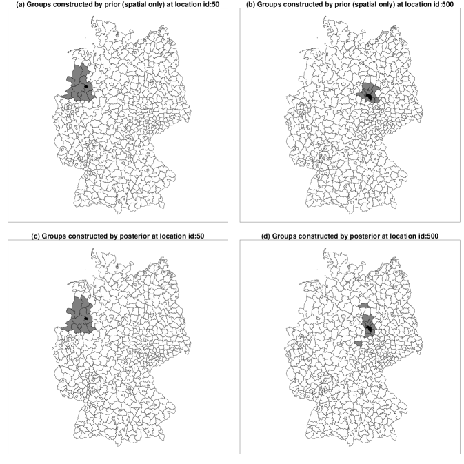
Figure 4: Groups by different automatic construction strategies. The testing point is located in the black region, and the data in the group are located in the grey regions. In (d), the group constructed by posteriors contains some non-spatial patterns.

Dengue Risk in Brazil

In this real-world example, we will demonstrate the scalability and adaptability of the automatic LGOCV method in a complex model structure and a large sample size. The automatically constructed groups are consistent with the domain knowledge that dengue disease is prevalent in summer.

We will repeat the variable selection process as shown in [18] using the automatic LGOCV. The model chosen by LGOCV is considered to have better predictive power than those selected based on other criteria because the most informative data points for predicting the target are excluded from the training set.

The models study the influence of extreme hydrometeorological hazards on dengue risk, factoring in Brazil’s urbanization levels. Our dataset, with $127,224$ samples representing $12,895,293$ dengue cases, covers Brazil’s 558 microregions from January 2001 to December 2019. Given the dataset’s magnitude and the model’s intricacy, LGOCV or LOOCV calculations require the approximation method detailed in Section 4.

Data points include month, year, microregion, and state. The candidate covariates encompass the monthly average of daily minimum ($T_{min}$) and maximum temperatures ($T_{max}$), the palmer drought severity index (PDSI), the urbanization levels: overall ($u$), centered at high ($u_{1}$), intermediate ($u_{2}$), and more rural levels ($u_{3}$) and the access to water supply: overall ($w$) and centered at high-frequency shortages ($w_{1}$), intermediate ($w_{2}$), and low-frequency shortages ($w_{3}$). For preprocessing specifics of these covariates, refer to [23].

The likelihood of the model is chosen to be negative binomial to account for overdispersion. The latent field consists of a temporal component describing a state-specific seasonality using a cyclic first difference prior distribution and a spatial component describing year-specific spatially unstructured and structured random effects using a modified Besag-York-Mollie (BYM2) model with a scaled spatial component [24]. The temporal component has replications for each state, and the spatial component has replications for each year. We can express the base model using the INLA-style formula,

$$\begin{split}\text{y}\sim 1&+\text{covariates}+\text{f(month, model = ``rw1", replicate = state, cyclic = TRUE)}\\ &+\text{f(microregion, model = ``bym2", replicate = year)}.\end{split}$$

In short, we write this model as $\text{y}\sim 1+\text{covariates}+f_{t}+f_{s}.$ The number of parameters in this model is $21,567$ with $127,224$ observations for the full model. The appendix of [18] and its repository [23] provide full details about the models and data.

The model accounts for temporal effects with spatial replicates and spatial effects with temporal replicates, complicated by various constraints. Given its intricacy and the lack of a clear prediction task, crafting groups for LGOCV manually is challenging. Hence, utilizing our automatic group construction through posterior correlation is beneficial. For model comparisons, using the same groups across different models is recommended. The base model, which only incorporates structured components, is chosen for group building. Most automatic groups cluster data from the same year, location, and nearby months to the testing points. Figure 5 displays the relative month frequencies in the group, given the testing points correspond to a specific month. The chart suggests the first half-year data better informs predictions. Even in July and November testing points, the group frequently includes that data, aligning with the known prevalence of dengue during summer. See Figure 5 (c) and (d) for details.

The results of model selection using deviance information criterion (DIC), LOOCV, and LGOCV are presented in Table 1. The candidate models are those referenced in [23]. To transform equation 1 into a loss function, we calculated its negative value. It is worth noting that LOOCV values across various models exhibit high similarities, suggesting that these models’ interpolation capabilities are similar. This observation is reasonable because all models incorporate spatial and temporal effects that typically offer more predictive power than the covariates. The results obtained from LGOCV are particularly different because of the removal of informative data. This leads to weaker predictive power of the spatial and temporal effects. The importance of the covariates is highlighted as a result.

Index	Model	DIC	LOOCV	LGOCV
1	$\text{y}\sim 1+f_{t}+f_{s}$	3615.38	0.0151	0.0206
2	$\text{y}\sim 1+T_{min}+f_{t}+f_{s}$	1562.96	0.0064	0.0088
3	$\text{y}\sim 1+T_{max}+f_{t}+f_{s}$	2228.73	0.0091	0.0133
4	$\text{y}\sim 1+PDSI+f_{t}+f_{s}$	2167.12	0.0092	0.0126
5	$\text{y}\sim 1+PDSI+T_{min}+f_{t}+f_{s}$	160.43	0.0006	0.0012
6	$\text{y}\sim 1+PDSI+T_{max}+f_{t}+f_{s}$	900.65	0.0038	0.0057
7	$\text{y}\sim 1+PDSI+T_{min}+PDSI*u_{1}+u+f_{t}+f_{s}$	38.21	0.0002	0*
8	$\text{y}\sim 1+PDSI+T_{min}+PDSI*u_{2}+u+f_{t}+f_{s}$	39.13	0.0002	0*
9	$\text{y}\sim 1+PDSI+T_{min}+PDSI*u_{3}+u+f_{t}+f_{s}$	28.64	0.0002	0*
10	$\text{y}\sim 1+PDSI+T_{min}+PDSI*w_{1}+w+f_{t}+f_{s}$	6.68	0*	0.0005
11	$\text{y}\sim 1+PDSI+T_{min}+PDSI*w_{2}+w+f_{t}+f_{s}$	0*	0*	0.0005
12	$\text{y}\sim 1+PDSI+T_{min}+PDSI*w_{3}+w+f_{t}+f_{s}$	4.55	0*	0.0006
Note: We offset DIC by 826841.66, LOOCV by 3.2721 and LGOCV by 3.3763.

Table 1: Model selection results

Figure 5: Groups for testing points from a specific month. $y$-axis: relative frequency, $x$-axis: month of data measurement in groups. The first half-year data are more informative for prediction. As shown in (c) and (d), even in July and November, the group often includes data consistent with the known summer prevalence of dengue.

6 Discussion

An over-reliance on LOOCV persists in statistical practice, despite concerns raised in studies like [4, 25]. To address this, we have introduced an automatic LGOCV designed to be convenient across various models and to provide a measure of predictive performance. Alongside this, we present an efficient approximation method for computation applicable to manually designed groups. We aim to steer statistical practice towards a better evaluation of predictive performance. It is pertinent to note that our automatic LGOCV do not replace a custom CV strategy designed by modelers tailored for specific applications. Yet, offering an alternative default strategy that improves LOOCV is a significant advantage.

Appendix A On the computation of $\boldsymbol{\Sigma}_{\boldsymbol{\eta}_{I_{i}}}(\boldsymbol{\theta},\boldsymbol{y}_{-I_{i}})$ and $\boldsymbol{\mu}_{\boldsymbol{\eta}_{I_{i}}}(\boldsymbol{\theta},\boldsymbol{y}_{-I_{i}})$

In this section, we let $I_{i}$ be $I$ and drop $\boldsymbol{\theta}$ to simplify the notation. We have a random vector $\boldsymbol{\eta}_{I}|\boldsymbol{y}\sim N(\boldsymbol{\mu}_{\boldsymbol{\eta}_{I}}(\boldsymbol{y}),\boldsymbol{\Sigma}_{\boldsymbol{\eta}_{I}}(\boldsymbol{y}))$, which can be viewed as a posterior distribution with prior $\boldsymbol{\eta}_{I}|\boldsymbol{y}_{-I}\sim N(\boldsymbol{\mu}_{\boldsymbol{\eta}}(\boldsymbol{y}_{-I}),\boldsymbol{\Sigma}_{\boldsymbol{\eta}}(\boldsymbol{y}_{-I}))$ and likelihood $\pi_{G}(\boldsymbol{y}_{I}|\boldsymbol{\eta}_{I})\propto\exp\bigg{\{}-\frac{1}{2}\boldsymbol{\eta}_{I}^{T}\boldsymbol{C}(\boldsymbol{y}_{I})\boldsymbol{\eta}_{I}+\boldsymbol{b}(\boldsymbol{y}_{I})\boldsymbol{\eta}_{I}\bigg{\}}$. Now, we need to use the posterior and the likelihood to obtain the prior.

If $\boldsymbol{\Sigma}_{\boldsymbol{\eta}_{I}}(\boldsymbol{y})$ is full rank, we have $\boldsymbol{Q}_{\boldsymbol{\eta}_{I}}(\boldsymbol{y})=\boldsymbol{\Sigma}_{\boldsymbol{\eta}_{I}}(\boldsymbol{y})^{-1}$ and $\boldsymbol{b}_{\boldsymbol{\eta}_{I}}(\boldsymbol{y})=\boldsymbol{Q}_{\boldsymbol{\eta}_{I}}(\boldsymbol{y})\boldsymbol{\mu}_{\boldsymbol{\eta}_{I}}(\boldsymbol{y})$. By conjugacy of Gaussian prior and Gaussian likelihood, $\boldsymbol{Q}_{\boldsymbol{\eta}_{I}}(\boldsymbol{y}_{-I})=\boldsymbol{Q}_{\boldsymbol{\eta}_{I}}(\boldsymbol{y})-\boldsymbol{C}(\boldsymbol{y}_{I})$ and $\boldsymbol{b}_{\boldsymbol{\eta}_{I}}(\boldsymbol{y}_{-I})=\boldsymbol{Q}_{\boldsymbol{\eta}_{I}}(\boldsymbol{y})\boldsymbol{\mu}_{\boldsymbol{\eta}_{I}}(\boldsymbol{y})-\boldsymbol{b}(\boldsymbol{y}_{I})$. Then we have desired $\boldsymbol{\mu}_{\boldsymbol{\eta}_{I}}(\boldsymbol{y}_{-I})$ and $\boldsymbol{\Sigma}_{\boldsymbol{\eta}_{I}}(\boldsymbol{y}_{-I})$.

If $\boldsymbol{\Sigma}_{\boldsymbol{\eta}_{I}}(\boldsymbol{y})$ is singular, we let $\boldsymbol{\eta}|\boldsymbol{y}=\boldsymbol{B}\boldsymbol{z}|\boldsymbol{y}$, where $\boldsymbol{B}=\boldsymbol{V}\boldsymbol{\Lambda}$ with $\boldsymbol{V}$ containing eigenvectors corresponding to non-zero eigenvalues, $\boldsymbol{\Lambda}$ containing square root of non-zero eigenvalues on its diagonal, and $\boldsymbol{z}|\boldsymbol{y}\sim N(\boldsymbol{\mu}_{\boldsymbol{z}}(\boldsymbol{y}),\boldsymbol{\mathcal{I}})$, where $\boldsymbol{\mathcal{I}}$ is an identity matrix and $\boldsymbol{\mu}_{\boldsymbol{z}}(\boldsymbol{y})=\boldsymbol{B}^{T}\boldsymbol{\mu}_{\boldsymbol{\eta}_{I}}(\boldsymbol{y})$. By conjugacy, we have $\boldsymbol{Q}_{\boldsymbol{z}}(\boldsymbol{y}_{-I})=\boldsymbol{\mathcal{I}}-\boldsymbol{B}^{T}\boldsymbol{C}(\boldsymbol{y}_{I})\boldsymbol{B}$ and $\boldsymbol{b}_{\boldsymbol{z}}(\boldsymbol{y}_{-I})=\boldsymbol{\mu}_{\boldsymbol{z}}(\boldsymbol{y})-\boldsymbol{B}^{T}\boldsymbol{b}(\boldsymbol{y}_{I})$. It is followed by $\boldsymbol{\mu}_{\boldsymbol{z}}(\boldsymbol{y}_{-I})=\boldsymbol{Q}_{\boldsymbol{z}}(\boldsymbol{y}_{-I})^{-1}\boldsymbol{b}_{\boldsymbol{z}}(\boldsymbol{y}_{-I})$. Then mean and covariance of $\boldsymbol{z}|\boldsymbol{y}_{-I}$ is $\boldsymbol{\mu}_{\boldsymbol{\eta}}(\boldsymbol{y}_{-I})=\boldsymbol{B}\boldsymbol{\mu}_{\boldsymbol{z}}(\boldsymbol{y}_{-I})$, $\boldsymbol{\Sigma}_{\boldsymbol{\eta}}(\boldsymbol{y}_{-I})=\boldsymbol{B}\boldsymbol{\Sigma}_{\boldsymbol{z}}(\boldsymbol{y}_{-I})\boldsymbol{B}^{T}$.

Appendix B On the computation of $\boldsymbol{\Sigma}_{\boldsymbol{\eta}_{I_{i}}}(\boldsymbol{\theta},\boldsymbol{y})$ and $\boldsymbol{\mu}_{\boldsymbol{\eta}_{I_{i}}}(\boldsymbol{\theta},\boldsymbol{y})$ with Linear Constraints

We start by illustrating how to compute $\boldsymbol{\Sigma}_{\boldsymbol{\eta}_{I_{i}}}(\boldsymbol{\theta},\boldsymbol{y})$ and $\boldsymbol{\mu}_{\boldsymbol{\eta}_{I_{i}}}(\boldsymbol{\theta},\boldsymbol{y})$ without linear constraints. $\boldsymbol{\mu}_{\boldsymbol{\eta}_{I_{i}}}(\boldsymbol{\theta},\boldsymbol{y})$ is simply obtained by $\boldsymbol{\mu}_{\boldsymbol{\eta}_{I_{i}}}(\boldsymbol{\theta},\boldsymbol{y})=\boldsymbol{A}_{I_{i}}\boldsymbol{\mu}_{\boldsymbol{f}}(\boldsymbol{\theta},\boldsymbol{y})$. However, we never store large dense matrix like $\boldsymbol{Q}_{\boldsymbol{f}}(\boldsymbol{\theta},\boldsymbol{y})^{-1}$. Thus, $\boldsymbol{\Sigma}_{\boldsymbol{\eta}_{I_{i}}}(\boldsymbol{\theta},\boldsymbol{y})$ cannot be obtained by using matrix multiplication $\boldsymbol{A}_{I_{i}}\boldsymbol{Q}_{\boldsymbol{f}}(\boldsymbol{\theta},\boldsymbol{y})^{-1}\boldsymbol{A}_{I_{i}}^{T}$. Instead, we compute $\boldsymbol{\Sigma}_{\boldsymbol{\eta}}(\boldsymbol{\theta},\boldsymbol{y})$ entry by entry and use the result to fill in entries of $\boldsymbol{\Sigma}_{\boldsymbol{\eta}_{I_{i}}}(\boldsymbol{\theta},\boldsymbol{y})$. We compute $\boldsymbol{\Sigma}_{\boldsymbol{\eta}}(\boldsymbol{\theta},\boldsymbol{y})_{i,j}$ by solving

$$\boldsymbol{Q}_{\boldsymbol{f}}(\boldsymbol{\theta},\boldsymbol{y})\boldsymbol{x}=\boldsymbol{A_{i}}$$

and $\boldsymbol{\Sigma}_{\boldsymbol{\eta}}(\boldsymbol{\theta},\boldsymbol{y})_{i,j}=\boldsymbol{A_{j}}\boldsymbol{x}$. The computation is fast because $\boldsymbol{A}$ and $\boldsymbol{Q}_{\boldsymbol{f}}(\boldsymbol{\theta},\boldsymbol{y})$ are sparse, and the factorization of $\boldsymbol{Q}_{\boldsymbol{f}}(\boldsymbol{\theta},\boldsymbol{y})$ is reused.

When linear constraints $\boldsymbol{\mathcal{C}}\boldsymbol{f}=\boldsymbol{e}$ are applied on $\boldsymbol{f}$, we have

$$\begin{split}&\boldsymbol{\Sigma}_{\boldsymbol{f}}(\boldsymbol{\theta},\boldsymbol{y})^{*}=\boldsymbol{Q}_{\boldsymbol{f}}(\boldsymbol{\theta},\boldsymbol{y})^{-1}-\boldsymbol{Q}_{\boldsymbol{f}}(\boldsymbol{\theta},\boldsymbol{y})^{-1}\boldsymbol{\mathcal{C}}^{T}(\boldsymbol{\mathcal{C}}\boldsymbol{Q}_{\boldsymbol{f}}(\boldsymbol{\theta},\boldsymbol{y})^{-1}\boldsymbol{\mathcal{C}}^{T})^{-1}\boldsymbol{\mathcal{C}}\boldsymbol{Q}_{\boldsymbol{f}}(\boldsymbol{\theta},\boldsymbol{y})^{-1},\\ &\boldsymbol{\mu}_{\boldsymbol{f}}(\boldsymbol{\theta},\boldsymbol{y})^{*}=\boldsymbol{\mu}_{\boldsymbol{f}}(\boldsymbol{\theta},\boldsymbol{y})-\boldsymbol{Q}_{\boldsymbol{f}}(\boldsymbol{\theta},\boldsymbol{y})^{-1}\boldsymbol{\mathcal{C}}^{T}(\boldsymbol{\mathcal{C}}\boldsymbol{Q}_{\boldsymbol{f}}(\boldsymbol{\theta},\boldsymbol{y})^{-1}\boldsymbol{\mathcal{C}}^{T})^{-1}(\boldsymbol{\mathcal{C}}\boldsymbol{\mu}_{\boldsymbol{f}}-\boldsymbol{e}),\end{split}$$

where $\boldsymbol{\Sigma}_{\boldsymbol{f}}(\boldsymbol{\theta},\boldsymbol{y})^{*}$ and $\boldsymbol{\mu}_{\boldsymbol{f}}(\boldsymbol{\theta},\boldsymbol{y})^{*}$ are the mean and the covariance matrix after applying constraints [16]. Because $\boldsymbol{\mu}_{\boldsymbol{f}}(\boldsymbol{\theta},\boldsymbol{y})^{*}$, is always stored, the computation of $\boldsymbol{\mu}_{\boldsymbol{\eta}_{I_{i}}}(\boldsymbol{\theta},\boldsymbol{y})$ is simple. We need to propagate the effects of linear constraints to $\boldsymbol{\Sigma}_{\boldsymbol{\eta}}(\boldsymbol{\theta},\boldsymbol{y})_{i,j}$. This is achieved by computing [16]

$$\boldsymbol{x}^{*}=\boldsymbol{x}-\boldsymbol{Q}_{\boldsymbol{f}}(\boldsymbol{\theta},\boldsymbol{y})^{-1}\boldsymbol{\mathcal{C}}^{T}(\boldsymbol{\mathcal{C}}\boldsymbol{Q}_{\boldsymbol{f}}(\boldsymbol{\theta},\boldsymbol{y})^{-1}\boldsymbol{\mathcal{C}}^{T})^{-1}\boldsymbol{\mathcal{C}}\boldsymbol{x},$$

where $\boldsymbol{x}$ solves $\boldsymbol{Q}_{\boldsymbol{f}}(\boldsymbol{\theta},\boldsymbol{y})\boldsymbol{x}=\boldsymbol{A_{i}}$. Then $\boldsymbol{\Sigma}_{\boldsymbol{\eta}}(\boldsymbol{\theta},\boldsymbol{y})^{*}_{i,j}=\boldsymbol{A_{j}}\boldsymbol{x}^{*}.$

References

• [1] Mervyn Stone. Cross-validatory choice and assessment of statistical predictions. Journal of the royal statistical society: Series B (Methodological), 36(2):111–133, 1974.
• [2] Tilmann Gneiting and AdrianΒ E Raftery. Strictly proper scoring rules, prediction, and estimation. Journal of the American statistical Association, 102(477):359–378, 2007.
• [3] Sohrab Saeb, Luca Lonini, Arun Jayaraman, DavidΒ C Mohr, and KonradΒ P Kording. The need to approximate the use-case in clinical machine learning. Gigascience, 6(5):gix019, 2017.
• [4] DavidΒ R Roberts, Volker Bahn, Simone Ciuti, MarkΒ S Boyce, Jane Elith, Gurutzeta Guillera-Arroita, Severin Hauenstein, José J Lahoz-Monfort, Boris SchrΓΆder, Wilfried Thuiller, etΒ al. Cross-validation strategies for data with temporal, spatial, hierarchical, or phylogenetic structure. Ecography, 40(8):913–929, 2017.
• [5] Paul-Christian BΓΌrkner, Jonah Gabry, and Aki Vehtari. Approximate leave-future-out cross-validation for bayesian time series models. Journal of Statistical Computation and Simulation, 90(14):2499–2523, 2020.
• [6] Andrew Gelman, JohnΒ B Carlin, HalΒ S Stern, and DonaldΒ B Rubin. Bayesian data analysis. Chapman and Hall/CRC, 1995.
• [7] Hvard Rue, Sara Martino, and Nicolas Chopin. Approximate bayesian inference for latent gaussian models by using integrated nested laplace approximations. Journal of the royal statistical society: Series b (statistical methodology), 71(2):319–392, 2009.
• [8] Hvard Rue, Andrea Riebler, SigrunnΒ H SΓΈrbye, JanineΒ B Illian, DanielΒ P Simpson, and FinnΒ K Lindgren. Bayesian computing with inla: a review. Annual Review of Statistics and Its Application, 4:395–421, 2017.
• [9] Janet van Niekerk and Haavard Rue. Correcting the laplace method with variational bayes. arXiv preprint arXiv:2111.12945, 2021.
• [10] Janet VanΒ Niekerk, Elias Krainski, Denis Rustand, and Hvard Rue. A new avenue for bayesian inference with inla. Computational Statistics & Data Analysis, 181:107692, 2023.
• [11] Assaf Rabinowicz and Saharon Rosset. Cross-validation for correlated data. Journal of the American Statistical Association, pages 1–14, 2020.
• [12] Prabir Burman, Edmond Chow, and Deborah Nolan. A cross-validatory method for dependent data. Biometrika, 81(2):351–358, 1994.
• [13] Xiaofeng Wang, YuΒ Ryan Yue, and JulianΒ J Faraway. Bayesian regression modeling with INLA. CRC Press, 2018.
• [14] Elias Krainski, Virgilio GΓ³mez-Rubio, Haakon Bakka, Amanda Lenzi, Daniela Castro-Camilo, Daniel Simpson, Finn Lindgren, and Hvard Rue. Advanced spatial modeling with stochastic partial differential equations using R and INLA. Chapman and Hall/CRC, 2018.
• [15] Virgilio GΓ³mez-Rubio. Bayesian inference with INLA. CRC Press, 2020.
• [16] Havard Rue and Leonhard Held. Gaussian Markov random fields: theory and applications. Chapman and Hall/CRC, 2005.
• [17] Qing Liu and DonaldΒ A Pierce. A note on gaussβ€”hermite quadrature. Biometrika, 81(3):624–629, 1994.
• [18] Rachel Lowe, SophieΒ A Lee, KathleenΒ M O’Reilly, OliverΒ J Brady, Leonardo Bastos, Gabriel Carrasco-Escobar, Rafael deΒ CastroΒ CatΓ£o, FelipeΒ J ColΓ³n-GonzΓ‘lez, Christovam Barcellos, MariliaΒ SΓ‘ Carvalho, etΒ al. Combined effects of hydrometeorological hazards and urbanisation on dengue risk in brazil: a spatiotemporal modelling study. The Lancet Planetary Health, 5(4):e209–e219, 2021.
• [19] Stan Development Team. RStan: the R interface to Stan, 2022. R package version 2.21.5.
• [20] Julian Besag, Jeremy York, and Annie MolliΓ©. Bayesian image restoration, with two applications in spatial statistics. Annals of the institute of statistical mathematics, 43(1):1–20, 1991.
• [21] JonathanΒ C Wakefield, NGΒ Best, and LΒ Waller. Bayesian approaches to disease mapping. Spatial epidemiology: methods and applications, pages 104–127, 2000.
• [22] Leonhard Held, Isabel NatΓ‘rio, SarahΒ Elaine Fenton, Hvard Rue, and Nikolaus Becker. Towards joint disease mapping. Statistical methods in medical research, 14(1):61–82, 2005.
• [23] Rachel Lowe. Data and R code to accompany ’Combined effects of hydrometeorological hazards and urbanisation on dengue risk in Brazil: a spatiotemporal modelling study’, March 2021.
• [24] Andrea Riebler, SigrunnΒ H SΓΈrbye, Daniel Simpson, and Hvard Rue. An intuitive bayesian spatial model for disease mapping that accounts for scaling. Statistical methods in medical research, 25(4):1145–1165, 2016.
• [25] Aki Vehtari, DanielΒ P Simpson, Yuling Yao, and Andrew Gelman. Limitations of β€œlimitations of bayesian leave-one-out cross-validation for model selection”. Computational Brain & Behavior, 2(1):22–27, 2019.