Search for anisotropic, birefringent spacetime-symmetry breaking in gravitational wave propagation from GWTC-3
Abstract
An effective field theory framework, the Standard-Model Extension, is used to investigate the existence of Lorentz and CPT-violating effects during gravitational wave propagation. We implement a modified equation for the dispersion of gravitational waves, that includes isotropic, anisotropic and birefringent dispersion. Using the LIGO-Virgo-KAGRA algorithm library suite, we perform a joint Bayesian inference of the source parameters and coefficients for spacetime symmetry breaking. From a sample of 45 high confidence events selected in the GWTC-3 catalog, we obtain a maximal bound of m at 90% CI for the isotropic coefficient when assuming the anisotropic coefficients to be zero. The combined measurement of all the dispersion parameters yields limits on the order of m for the 16 coefficients. We study the robustness of our inference by comparing the constraints obtained with different waveform models, and find that a lack of physics in the simulated waveform may appear as spacetime symmetry breaking-induced dispersion for a subset of events.
I Introduction
In the search for a fundamental unified theory of physics, it may be imperative to reconsider the axioms underlying General Relativity (GR)and the Standard Model (SM)of particle physics. Many theoretical proposals argue for a possible breaking of spacetime symmetries, including Lorentz invariance (LI)and Charge-Parity-Time (CPT)symmetry [1, 2, 3, 4, 5, 6], in such a way that it may be detectable in sensitive tests. The direct detections of gravitational waves (GWs)reported by the LIGO-Virgo-KAGRA (LVK)collaboration provide a new channel to test the rich phenomenology induced by spacetime-symmetry breaking in the gravitation sector [7, 8, 9, 10, 11].
The effective field theory referred to as the Standard-Model Extension (SME)is a theoretical framework dedicated to derive the observable consequences of spacetime-symmetry breaking that is punctilious and model independent. The framework is comprised of the action of GR and the SM plus all possible terms obtainable from GR and SM field operators contracted with coefficients for spacetime-symmetry breaking, including local Lorentz, CPT, and diffeomorphism breaking terms [12, 13, 14, 15, 16, 17, 18, 19, 20, 21]. Extensive constraints have been derived on these terms within the matter sector and in the gravity sector [22], the latter having been studied with a wide range of astrophysical probes [15, 19, 20, 23, 24, 25]. Existing analysis includes short-range gravity tests [26, 27, 28], gravimetry tests [29, 30, 31, 32, 33, 34, 35], astrophysical tests with pulsars [36, 37, 38], solar system planetary tests [39, 40, 41], near-Earth tests [42, 43, 44, 45], and tests with GWs [46, 19, 47, 48, 49, 50, 51]. We complement those searches with further study of the LI and CPT-violating effects on propagation of GW. We use dynamical equations for the metric fluctuations derived from the action of the SME, and the resulting effects include dispersion, anisotropy, and birefringence.
Several tests of GR have been performed with the GW events detected by the LVK [47, 48, 52, 49, 50, 53, 54]. Some related works focus on parameterizations of the deviations from GR [9, 10, 55, 56], including waveform consistency tests, modification of the GW generation, presence of extra polarization modes, and tests using specific models [57, 58, 59, 60, 61, 55, 62]. The current searches for LI violation performed by the LVK collaboration notably rely on a modified dispersion relation that includes isotropic and polarization-independent effects [53, 63, 64]. Using the SME framework, we extend this phenomenology by measuring the coefficients for LI and CPT violation, including anisotropic and polarization-dependent dispersion. First estimates of those coefficients have been derived using posterior probabilities released with previous GW catalog releases, effectively neglecting the correlations between the parameters describing the source and the spacetime-symmetry breaking coefficients [49, 50]. In this article, we present a joint measurement of the source parameters and the coefficients, alongside studying the robustness of the results we obtain.
Section II summarizes the derivation of the phenomenology induced by LI and CPT violation in the SME framework. Section III details the methodological aspects, including the dataset used for the measurement of the spacetime-symmetry breaking coefficients. Section IV presents the obtained results, as well as a discussion of the impact of the underlying gravitational waveform model and correlations with source parameters. Section V discusses those results in light of existing studies and future GW instrument sensitivities. Theoretical portions of this paper work with natural units, where and Newton’s gravitational constant is , while our data analysis work follows SI units. Greek letters are used for spacetime indices while Latin letters for spatial indices. We work with the spacetime metric signature .
II Theoretical derivation of a dispersion relation for gravitational waves
We summarize previous derivations in [19, 65, 66], focusing on gravity-sector terms within the SME framework. The spacetime metric is expanded as fluctuations about the Minkowski metric, , and we consider up to second order in for the action, which is sufficient to characterize propagation effects. This gives the following action:
| (1) |
The operator , consists of partial derivatives that act on ,
| (2) |
and are general background coefficients that are considered small, constant and control the size of any Lorentz or CPT violation;
Ensuring linearized gauge symmetry, i.e., , and retaining only terms that contribute to the resulting field equations, we arrive at the following Lagrange density [19]:
| (3) | |||||
The first term is the standard GR term written with the totally antisymmetric Levi-Civita tensor density , and the remaining terms contain all additional Lorentz invariant and violating terms, organized into three terms based on symmetry properties: is CPT even with mass dimension ; is CPT odd with mass dimension ; is CPT even with mass dimension . Details of these terms including the corresponding Young Tableaux can be found in Table 1 of Ref. [19]. As an example, for mass dimension ,
| (4) |
where has independent components. Note that the gauge symmetry requirement can be relaxed [20, 67], but we do not consider such terms here. The origin of the effective action for resulted from explicit symmetry breaking or spontaneous-symmetry breaking as discussed elsewhere [15, 68, 19, 69].
Performing the variation with respect to on the action (3), results in the vacuum field equations,
| (5) | |||||
Assuming plane wave solutions, , where is spacetime position and is the four-momentum for the plane wave, and transforming into momentum space with the dispersion relation can be obtained independently of gauge conditions, as shown in references [70, 20]. The dispersion relation for the two propagating modes is given by
| (6) |
where
| (7) |
and
| (8) | |||||
We retrieve the GR case when symmetry-breaking coefficients, i.e. and , vanish. Note that this result holds at leading order in the coefficients for Lorentz violation, hence higher modes do not contribute in this perturbative treatment [70, 20]. Relaxing some of the assumptions in this framework, allowing for other fields to contribute dynamically to the action, could result in additional modes [71, 72].
GR predicts two linearly independent polarizations for GWs propagating in vacuum, traveling at the speed of light. Possible modifications for observable Lorentz and CPT violating effects from (6) include birefringence, e.g., altered relative travel speeds between the polarizations, which result from the two possible signs for in (6), requiring a minimum mass dimension . Furthermore, the presence of higher powers of frequency and momentum in the terms above, indicates beyond GR dispersion as well. All of these effects depend on the sky location of the propagating wave, and thus a breaking of rotational isotropy occurs.
To take into account the sky localization dependence of the source in the detector frame, it is advantageous to project the SME coefficients onto spherical harmonics [70],
| (9) | |||||
| (10) | |||||
| (11) |
where , the are the standard spherical harmonics while are spin-weighted spherical harmonics, and .
Expressions for the two linearly independent GW polarizations, in the transverse-traceless gauge, result in a phase shift from the additional symmetry-breaking effects,
| (12) | |||||
where
and the modified redshift becomes
| (13) |
For notational convenience, the angles in (12) are defined by the expressions below,
| (14) |
One of the key features of spacetime symmetry breaking, as evidenced in the equations above, is the breaking of isotropy. The strength of the LI violation can change with source location [66]. Unless otherwise stated, the spherical coefficients in (9)-(11) are expressed in the Sun-Centered Celestial Equatorial reference frame (SCF), as is standard in the literature [73, 22], and allows comparisons with other non-GW tests in the gravity sector. Rotations and boosts of the spherical coefficients relative to this frame must be taken into account, as discussed elsewhere [74].
III Data and parameter inference
III.1 Bayesian inference of source and symmetry-breaking parameters
For mass dimension , LI violation leads to a modification of the GW group velocity that can be measured with multimessenger signals; constraints on the operator of Eq. (3) have been obtained from the observation of GW170817/GRB170817A [47] comparing light and GW travel time, and travel time across the Earth [48].
In this analysis, we focus on the coefficients for Lorentz and CPT violation contained in the operator for (see Eq (5)), with the first mass dimension in the action series (3) where GW dispersion occurs. We probe the impact of isotropic and anisotropic dispersion, as well as birefringence, with a joint estimation of the source parameters and the a priori independent coefficients of Eq. (11). Specifically, we are considering in this work, a subset of (12), where . In this case the remaining coefficients are contained in . The expression is lengthy but takes the form [66]:
| (15) | |||||
with the superscript meaning all quantities are evaluated with like equation (13).
Using a Bayesian inference framework, we compare the strain detected by the LVK interferometers with a template bank of gravitational waveforms modified as outlined in Eq. (12). The strain takes the form,
| (16) |
where are the expressions (12), and are the standard detector response functions. The rotation angles relating different frames, are included in the expressions for . These are defined in the LALSuite software, including the source frame and the detector frame. Again, the coefficients in (15) are left in the SCF.
We use the LALSuite algorithm package, modifying the LALSimulation subpackage to generate dispersed waveforms and performing the parameter estimation with a custom version of LALInference [75]. For a single event, LALInference evaluates the posterior probability with a Markov chain process using the matched-filtered likelihood:
| (17) | |||||
where is the template signal, is the interferometer datastream, is the duration of the signal, and the power spectral density (PSD)of the detector noise. Included in the vector set of GR prior parameters , are the intrinsic parameters describing the binary system (e.g. the masses and spins), as well as the (extrinsic) astrophysical environment parameters (e.g. the sky location, distance, inclination). The additional parameters , contain the SME coefficients .
The analysis is performed in the frequency domain, as detailed in [66]. The configurations of the Bayesian inferences, including the Markov chain algorithms and parameters, PSD and calibration envelops, are the same as the ones used by the LVK collaboration for parameter estimation. They are retrieved with the PESummary package [76], selecting the options associated with the IMRPhenomPv2 waveform model [77].
For each GW event, we first measure the isotropic dispersion coefficient , by taking a limiting case of (15) where we temporarily ignore the sky angle dependence and assume a flat prior on the SME coefficient. We then combine individual posterior probability densities to obtain a measurement of the 16 anisotropic coefficients while taking into account the source sky localization via the full expression in (15). We perform the combination by interpreting the sampled parameter as the linear combination:
| (18) |
where is the vector of N=45 posteriors of , is the matrix of spherical harmonics with and the sky coordinates, and corresponds to the n=16 SME coefficients. To invert Eq. (18) while the dimensions of the vectors and are unequal,the matrix of size can be decomposed with the Singular Value Decomposition (SVD)method:
| (19) |
where is a matrix of the orthonormal eigenvectors, is a diagonal matrix of the square root of the eigenvalues, and is the transpose of the matrix of the orthonormal eigenvectors. The elements are the singular values , chosen to be in decreasing order : . Inverting Eq. (19) results in:
| (20) |
which is equivalent to performing the linear least square minimization of , as done in the mesurement of without joint inference of the source parameters [78, 49]. We highlight that the results obtained with this method may differ from other type of multi-parameter inference, such as inferring the coefficients from multiple events at the time (currently infeasible due to the long sampling time it requires) or using Bayesian hierarchical inference. We chose this method motivated by two aspects: (i) to compare our results with previous estimates, highlighting the differences due to the joint inference of source and symmetry breaking parameters, and (ii) realising that due to the dimensionality and ordering of the matrix, this method effectively put more weight on the 16 events performing the best combination of parameters, effectively leading to an “optimal” estimate.
III.2 Dataset from the GWTC-3 catalog
We perform our analysis on the events detected during the three first observing runs, corresponding to the cumulative catalog GWTC-3 [11]. All the GW detections originate from the coalescence of binary systems of black holes and/or neutron stars, and the catalog reports 90 events with a probability of astrophysical origin larger than 50%. The study of GW residual shows that after subtraction of the best-fitted waveforms assuming GR, the leftover signals are consistent with noise, indicating that deviations from GR are higher order terms inducing small modification of the signal morphology [53]. Therefore, low-sensitivity events are unsuited for tests of GR as they may lead to false apparent deviations due to transient noise or incomplete modelling of the gravitational waveform [79, 80]. To prevent such undesirable features, we add the following requirements: (i) the false alarm rate (FAR)must be lower than , in order to only use high-confidence signals; and (ii) the event must have been selected by the LVK to test the modified dispersion relation, as while we use a different theoretical framework and phenomenology, we are also performing a measurement of GW dispersion. The final selection contains 45 events (10 events first reported in GWTC-1, 23 events in GWTC-2, and 12 events in GWTC-3), with signal-to-noise ratio (SNR)comprised within [9.2; 26.8] and luminosity distances within Gpc.
IV Measuring spacetime symmetry breaking parameters
IV.1 Constraints with GWTC-3
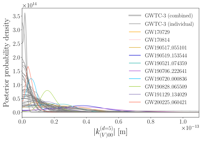
The marginalised posterior distribution of the isotropic dispersion coefficient is obtained for all the events described on Sec. III.2. As shown in Fig. 1, most events are compatible with a zero value of , corresponding to the GR case. The 68.3% upper bounds range between and according to the event, with 10 events presenting a 68.3% credible interval not compatible with GR. Only one event, GW190828_065509, is not compatible with GR at 90% CI. There have not been any transient noise (or “glitch”) requiring data quality mitigation recorded at the same time as the GW signals leading to a deviation, from GR, indicating that instrumental or environmental artifacts are unlikely to be the cause.
The combined constraint from all events on is m at 90% CI. At 68.3% CI, the combined bound is m. This deviation from GR is driven by the events GW190720_000836, GW190828_065509, GW200225_060421, and is alleviated when removing the three posteriors from the combination.
.
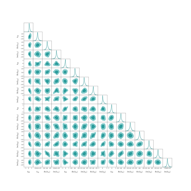
Using the fact that we have more individual events than coefficients, we perform a sky-localisation dependent analysis to extract the 16 coefficients from the posteriors, separating the anisotropic coefficients into real and imaginary components. Applying the SVD inverting method described on Sec. III.1, we obtain the posterior probabilities on the joint estimates shown in Fig. 2 alongside the correlations between the parameters. We note that during the combination of the posteriors from multiple events, information from the sky localisation distributions are transferred to the joint posteriors as explicited in Eq 18. The dimensionality reduction of the SVD method not being suitable to perform the common procedure of variable transform that would alleviate the effect of the non-flat prior, we observed the impact of the angular dependence by performing event-per-event single transformation of one parameter into another (e.g. to , assuming only one non-zero parameter at the time). Comparing posterior probability densities on for single events with and without a flat prior in , we noticed that the distributions were very similar and therefore the impact of the sky localisation prior negligible. The bounds on the spacetime symmetry breaking coefficients are extracted from the marginalised 1-dimensional posterior probability distributions displayed diagonally in Fig. 2, and summarised in Table 1. All the anisotropic coefficients are compatible with the GR case. The isotropic coefficient presents a deviation towards values superior to 0, driven by the events presenting a deviation in Fig. 1. When removing those 10 events, the deviation from GR does not appear anymore. The joint estimation is however less constraining than the individual one, as the bounds are three orders of magnitude larger than the combined constraint of individual events assuming the anisotropic coefficients to be zero.
| 90% | 68.3% | 68.3% | 90% | |
|---|---|---|---|---|
| lower | lower | coefficient | upper | upper |
| 0.51 | 1.21 | 4.38 | 7.37 | |
| -4.54 | -2.13 | 1.19 | 3.91 | |
| -2.30 | -1.00 | 1.73 | 3.39 | |
| -3.64 | -1.21 | 2.35 | 4.45 | |
| -7.40 | -3.75 | 1.10 | 3.78 | |
| -1.75 | -0.61 | 1.43 | 3.02 | |
| -2.77 | -1.16 | 1.71 | 3.67 | |
| -3.58 | -1.72 | 1.02 | 2.55 | |
| -2.49 | -0.96 | 2.80 | 5.58 | |
| -6.40 | -3.31 | 1.17 | 3.57 | |
| -3.34 | -1.65 | 0.98 | 2.48 | |
| -3.90 | -1.92 | 1.75 | 3.87 | |
| -2.76 | -1.23 | 1.34 | 2.87 | |
| -2.26 | -0.90 | 1.82 | 3.60 | |
| -3.95 | -1.95 | 1.28 | 3.18 | |
| -3.22 | -1.35 | 2.25 | 4.78 |
IV.2 Robustness tests
The events shown in color in Fig. 1 present a 68.3% CI not compatible with the GR case of m. We have surveyed the results presented by the LVK in their articles summarising several tests of GR to look for other pathological behaviour from those events [9, 10, 53]. We find two events from O2 (GW170729, GW170814) and two from O3 (GW190828_065509, GW200225_060421) that have been shown to drive a bias in the estimation of the modified dispersion relation parameters. Three O3 events (GW190519_153544, GW190521_074359, and GW190828_065509) present deviations in parameterised post-Newtonian tests, while one O3 event (GW200225_060421) presents poor score in residual tests. Those features indicate a lack of new physics in the model used to generate the GR parts and of Eq. (12), that may originate from the lack of dynamical effects of features of a new theory. The mismodeling or lack of modeling of dynamical phenomena, such as an approximation of precession or assuming circular orbits, can impact the estimation of beyond-GR parameters [80].
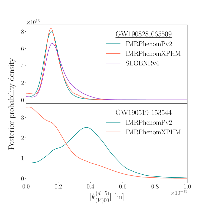
In order to investigate the robustness of the results, we inferred using different waveform models for several binary black hole events, as shown for two cases on Fig. 3. We compared the posterior probability densities obtained with IMRPhenomPv2 with the ones inferred with the SEOBNRv4, that uses an effective one-body description of the dynamics of spinning binaries [81]; and IMRPhenomXPHM, an updated version of IMRPhenomPv2 including higher harmonics and updated calibration to precession [82]. For the 23 events where we compared IMRPhenomPv2 and IMRPhenomXPHM, only four events showed a considerable modification of the credible intervals with a mode different from zero for only one of the model (GW190519_153544, GW190706_222641, GW200219_094415, GW200225_060421). For the four events where we compared IMRPhenomPv2 and SEOBNRv4, two presented a modification of the credible intervals (GW190630_185205, GW190720_000836). When investigating the events presenting a CI not including 0, only three of the ten events are compatible with the GR case with another model (GW190519_153544, GW190706_222641, GW190720_000836). While this rules out mismodelling as the unique source of tension, it points towards a lack of dynamics in the underlying model for some cases, and highlights the sensitivity of our analysis to spot deviations in GW signals. However, as waveform models share some common assumptions, and the uncertainty due to the modeling process (i.e., their mismatch with numerical relativity simulations) is not propagated during the analysis, more detailed study about waveform accuracy must be carried before ruling it out as a cause for apparent deviations from GR.
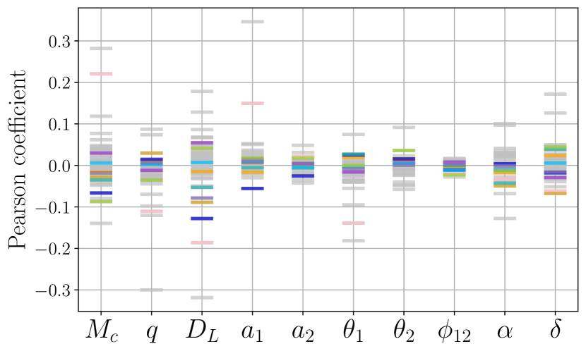
By measuring jointly the source and symmetry breaking parameters, the correlations between the variables are taken into account during the inference. We evaluate them by measuring the Pearson coefficients between and the source parameters as shown in Fig. 4, where the events presenting deviations from GR at 68.3% CI are highlighted. Most events show no or very moderate correlations, and amongst the highlighted events, while GW170814 and GW190519_153544 present large (anti)correlation with the mass and spin parameters, other events in agreement with GR present larger correlations. Those results indicate that a more accurate measurement of the source parameters, as could be obtained from higher SNR or from the detection of higher modes, can lead to an improvement of the constraints on the SME coefficients.
V Discussion
This work presents a new probe of Lorentz and CPT violation with GWs, extending the search for possible signals from a unified theory of physics. Our analysis relies on an effective field theory framework, which allows one to derive phenomenological consequences of spacetime-symmetry breaking across many regimes. This work complements existing parameterizations of LI violation in GWs. We extend the measurement of SME coefficients to higher mass dimension terms in the action, compared to constraints derived from speed of gravity tests, by probing GW dispersion, including anisotropic and birefringence effects. Our method goes beyond existing measurements by performing a joint inference of source parameters and symmetry-breaking coefficients, effectively taking into account correlations. Compared to SME measurements relying on time delay measurements, estimated from posterior probabilities inferred assuming GR, we find milder constraints on the order of instead of [49, 50]. These results indicate that correlations between GR and SME coefficients must be taken into account and the simplified treatments in earlier work should be replaced with proper parameter estimation.
While this work was carried, another team performed an independent measurement of SME coefficients for [51]. Our analysis differs by estimating the joint posterior probability for 16 coefficients, while they perform a measurement of single and dual coefficients only, assuming the remaining coefficients to be zero. Consequently, our analysis includes possible correlations between SME coefficients, as can be seen in Fig. 2. On the methodological side, our analysis relies on the LALInference software, while [51] relies on the bilby software. Using different methods enables us to verify the validity of the inferences provided by each software, and we find our results to be in agreement as we both derive a joint constraint around when assuming that all other coefficients are zero.
Note also that the main measurement results in this paper, the limits on coefficients in Table 1, can be directly compared to the results from other tests in gravity [22]. For example, solar-system tests like lunar laser ranging have yielded measurements on linear combinations of the independent mass dimension coefficients in in Eq. (3), with limits on the order of m [44]. This seems substantially poorer than the limits in this paper from GWs, but the coefficients probed in this paper are distinct linear combinations of the coefficients from those occurring in lunar laser ranging. Similarly, limits from pulsars via orbital tests are on the order of m [37], but probe distinct coefficients from GWs. Should a nonzero detection occur, it will be important to compare measurements in distinct tests.
While our global results are compatible with GR, a subset of events show non-zero estimates. We investigated possible shared features between those events, that do not display similar sky localisation neither other common parameters. Robustness tests indicate that for few events, the addition of higher modes resolves the tension. However, several events do not present modified posterior probability profiles when using other waveform models, pointing to the possibility that existing waveform models may lack dynamical features degenerate with the effects of dispersion. The current efforts in creating more accurate waveform templates, e.g. with the addition of eccentric trajectories, will provide a better understanding of the relevance of modelling accuracy for SME tests in particular and tests of GR in general.
The analysis in this paper studies propagation effects from LI violation. The addition of other possible effects from higher-order (in ) terms in the SME on the waveform itself, for example, via a post-Newtonian multipole expansion in the SME framework, could provide new tests. The latter work is in progess [24, 69].
Acknowledgements.
LH is supported by the Swiss National Science Foundation grant 199307, and by the European Union’s Horizon 2020 research and innovation programme under the Marie Skłodowska-Curie grant agreement No 945298-ParisRegionFP,. She is a Fellow of Paris Region Fellowship Programme supported by the Paris Region, and acknowledges the support of the COST Action CA18108. Work on this project by QGB and KOA was supported by the United States National Science Foundation (NSF) under grant numbers 1806871 and 2207734. Work on this project by JDT and MB was supported by the NSF under grant number 1806990. LS was supported by the National Natural Science Foundation of China (11975027, 11991053, 11721303), the National SKA Program of China (2020SKA0120300), and the Max Planck Partner Group Program funded by the Max Planck Society. The authors would like to thank the LIGO-Virgo-KAGRA collaboration for general support, and particularly Duncan MacLeod, Peter Tsun Ho Pang, Charlie Hoy, Geraint Pratten and John Veitch for the useful discussion concerning the software infrastructure. This research has made use of data or software obtained from the Gravitational Wave Open Science Center (gw-openscience.org), a service of LIGO Laboratory, the LIGO Scientific Collaboration, the Virgo Collaboration, and KAGRA. LIGO Laboratory and Advanced LIGO are funded by the NSF as well as the Science and Technology Facilities Council (STFC) of the United Kingdom, the Max-Planck-Society (MPS), and the State of Niedersachsen/Germany for support of the construction of Advanced LIGO and construction and operation of the GEO600 detector. Additional support for Advanced LIGO was provided by the Australian Research Council. Virgo is funded, through the European Gravitational Observatory (EGO), by the French Centre National de Recherche Scientifique (CNRS), the Italian Istituto Nazionale di Fisica Nucleare (INFN) and the Dutch Nikhef, with contributions by institutions from Belgium, Germany, Greece, Hungary, Ireland, Japan, Monaco, Poland, Portugal, Spain. The construction and operation of KAGRA are funded by Ministry of Education, Culture, Sports, Science and Technology (MEXT), and Japan Society for the Promotion of Science (JSPS), National Research Foundation (NRF) and Ministry of Science and ICT (MSIT) in Korea, Academia Sinica (AS) and the Ministry of Science and Technology (MoST) in Taiwan. The authors are grateful for computational resources provided by the LIGO Laboratory and supported by the NSF PHY-0757058 and PHY-0823459.References
- Kostelecký and Samuel [1989] V. A. Kostelecký and S. Samuel, Spontaneous breaking of lorentz symmetry in string theory, Phys. Rev. D 39, 683 (1989).
- Gambini and Pullin [1999] R. Gambini and J. Pullin, Nonstandard optics from quantum space-time, Phys. Rev. D 59, 124021 (1999).
- Carroll et al. [2001] S. M. Carroll, J. A. Harvey, V. A. Kostelecký, C. D. Lane, and T. Okamoto, Noncommutative field theory and lorentz violation, Phys. Rev. Lett. 87, 141601 (2001).
- Alan Kostelecký and Potting [1991] V. Alan Kostelecký and R. Potting, Cpt and strings, Nuclear Physics B 359, 545 (1991).
- Addazi et al. [2022] A. Addazi et al., Quantum gravity phenomenology at the dawn of the multi-messenger era—A review, Prog. Part. Nucl. Phys. 125, 103948 (2022), arXiv:2111.05659 [hep-ph] .
- Mariz et al. [2022] T. Mariz, J. R. Nascimento, and A. Y. Petrov, Lorentz symmetry breaking – classical and quantum aspects, (2022), arXiv:2205.02594 [hep-th] .
- Abbott et al. [2016a] B. P. Abbott et al. (LIGO Scientific, Virgo), Observation of Gravitational Waves from a Binary Black Hole Merger, Phys. Rev. Lett. 116, 061102 (2016a), arXiv:1602.03837 [gr-qc] .
- Abbott et al. [2016b] B. P. Abbott et al. (LIGO Scientific, Virgo), Tests of general relativity with GW150914, Phys. Rev. Lett. 116, 221101 (2016b), [Erratum: Phys.Rev.Lett. 121, 129902 (2018)], arXiv:1602.03841 [gr-qc] .
- Abbott et al. [2019a] B. P. Abbott et al. (LIGO Scientific, Virgo), Tests of General Relativity with the Binary Black Hole Signals from the LIGO-Virgo Catalog GWTC-1, Phys. Rev. D 100, 104036 (2019a), arXiv:1903.04467 [gr-qc] .
- Abbott et al. [2021a] R. Abbott et al. (LIGO Scientific, Virgo), Tests of general relativity with binary black holes from the second LIGO-Virgo gravitational-wave transient catalog, Phys. Rev. D 103, 122002 (2021a), arXiv:2010.14529 [gr-qc] .
- Abbott et al. [2021b] R. Abbott et al. (LIGO Scientific, VIRGO, KAGRA), GWTC-3: Compact Binary Coalescences Observed by LIGO and Virgo During the Second Part of the Third Observing Run, (2021b), arXiv:2111.03606 [gr-qc] .
- Colladay and Kostelecký [1997] D. Colladay and V. A. Kostelecký, violation and the standard model, Phys. Rev. D 55, 6760 (1997).
- Colladay and Kostelecký [1998] D. Colladay and V. A. Kostelecký, Lorentz-violating extension of the standard model, Phys. Rev. D 58, 116002 (1998).
- Kostelecký [2004] V. A. Kostelecký, Gravity, lorentz violation, and the standard model, Phys. Rev. D 69, 105009 (2004).
- Bailey and Kostelecký [2006] Q. G. Bailey and V. A. Kostelecký, Signals for lorentz violation in post-newtonian gravity, Phys. Rev. D 74, 045001 (2006).
- Kostelecky and Tasson [2011] V. A. Kostelecky and J. D. Tasson, Matter-gravity couplings and Lorentz violation, Phys. Rev. D 83, 016013 (2011), arXiv:1006.4106 [gr-qc] .
- Bailey et al. [2015] Q. G. Bailey, A. Kostelecký, and R. Xu, Short-range gravity and Lorentz violation, Phys. Rev. D 91, 022006 (2015), arXiv:1410.6162 [gr-qc] .
- Bluhm [2015] R. Bluhm, Explicit versus spontaneous diffeomorphism breaking in gravity, Phys. Rev. D 91, 065034 (2015).
- Kostelecký and Mewes [2016] V. A. Kostelecký and M. Mewes, Testing local lorentz invariance with gravitational waves, Phys. Lett. B 757, 510 (2016).
- Kostelecký and Mewes [2018] V. A. Kostelecký and M. Mewes, Lorentz and diffeomorphism violations in linearized gravity, Phys. Lett. B 779, 136 (2018).
- Kostelecký and Li [2021] V. A. Kostelecký and Z. Li, Backgrounds in gravitational effective field theory, Phys. Rev. D 103, 024059 (2021).
- Kostelecký and Russell [2011] V. A. Kostelecký and N. Russell, Data tables for lorentz and violation, Rev. Mod. Phys. 83, 11 (2011).
- Xu [2019] R. Xu, Modifications to Plane Gravitational Waves from Minimal Lorentz Violation, Symmetry 11, 1318 (2019), arXiv:1910.09762 [gr-qc] .
- Xu et al. [2021] R. Xu, Y. Gao, and L. Shao, Signatures of Lorentz Violation in Continuous Gravitational-Wave Spectra of Ellipsoidal Neutron Stars, Galaxies 9, 12 (2021), arXiv:2101.09431 [gr-qc] .
- Nascimento et al. [2021] J. R. Nascimento, A. Y. Petrov, and A. R. Vieira, On plane wave solutions in Lorentz-violating extensions of gravity, Galaxies 9, 32 (2021), arXiv:2104.01651 [gr-qc] .
- Long and Kostelecký [2015] J. C. Long and V. A. Kostelecký, Search for Lorentz violation in short-range gravity, Phys. Rev. D 91, 092003 (2015), arXiv:1412.8362 [hep-ex] .
- Shao et al. [2016] C.-G. Shao et al., Combined search for Lorentz violation in short-range gravity, Phys. Rev. Lett. 117, 071102 (2016), arXiv:1607.06095 [gr-qc] .
- Shao et al. [2019] C.-G. Shao, Y.-F. Chen, Y.-J. Tan, S.-Q. Yang, J. Luo, M. E. Tobar, J. C. Long, E. Weisman, and V. A. Kostelecký, Combined Search for a Lorentz-Violating Force in Short-Range Gravity Varying as the Inverse Sixth Power of Distance, Phys. Rev. Lett. 122, 011102 (2019), arXiv:1812.11123 [gr-qc] .
- Muller et al. [2008] H. Muller, S.-w. Chiow, S. Herrmann, S. Chu, and K.-Y. Chung, Atom Interferometry tests of the isotropy of post-Newtonian gravity, Phys. Rev. Lett. 100, 031101 (2008), arXiv:0710.3768 [gr-qc] .
- Chung et al. [2009] K.-Y. Chung, S.-w. Chiow, S. Herrmann, S. Chu, and H. Muller, Atom interferometry tests of local Lorentz invariance in gravity and electrodynamics, Phys. Rev. D 80, 016002 (2009), arXiv:0905.1929 [gr-qc] .
- Hohensee et al. [2011] M. A. Hohensee, S. Chu, A. Peters, and H. Muller, Equivalence Principle and Gravitational Redshift, Phys. Rev. Lett. 106, 151102 (2011), arXiv:1102.4362 [gr-qc] .
- Hohensee et al. [2013] M. A. Hohensee, H. Mueller, and R. B. Wiringa, Equivalence Principle and Bound Kinetic Energy, Phys. Rev. Lett. 111, 151102 (2013), arXiv:1308.2936 [gr-qc] .
- Flowers et al. [2017] N. A. Flowers, C. Goodge, and J. D. Tasson, Superconducting-Gravimeter Tests of Local Lorentz Invariance, Phys. Rev. Lett. 119, 201101 (2017), arXiv:1612.08495 [gr-qc] .
- Shao et al. [2018] C.-G. Shao, Y.-F. Chen, R. Sun, L.-S. Cao, M.-K. Zhou, Z.-K. Hu, C. Yu, and H. Müller, Limits on Lorentz violation in gravity from worldwide superconducting gravimeters, Phys. Rev. D 97, 024019 (2018), arXiv:1707.02318 [gr-qc] .
- Ivanov et al. [2019] A. N. Ivanov, M. Wellenzohn, and H. Abele, Probing of violation of Lorentz invariance by ultracold neutrons in the Standard Model Extension, Phys. Lett. B 797, 134819 (2019), arXiv:1908.01498 [hep-ph] .
- Shao [2014] L. Shao, Tests of local Lorentz invariance violation of gravity in the standard model extension with pulsars, Phys. Rev. Lett. 112, 111103 (2014), arXiv:1402.6452 [gr-qc] .
- Shao and Bailey [2018] L. Shao and Q. G. Bailey, Testing velocity-dependent CPT-violating gravitational forces with radio pulsars, Phys. Rev. D 98, 084049 (2018), arXiv:1810.06332 [gr-qc] .
- Wex and Kramer [2020] N. Wex and M. Kramer, Gravity Tests with Radio Pulsars, Universe 6, 156 (2020).
- Iorio [2012] L. Iorio, Orbital effects of Lorentz-violating Standard Model Extension gravitomagnetism around a static body: a sensitivity analysis, Class. Quant. Grav. 29, 175007 (2012), arXiv:1203.1859 [gr-qc] .
- Hees et al. [2013] A. Hees, B. Lamine, S. Reynaud, M. T. Jaekel, C. Le Poncin-Lafitte, V. Lainey, A. Fuzfa, J. M. Courty, V. Dehant, and P. Wolf, Simulations of Solar System observations in alternative theories of gravity, in 13th Marcel Grossmann Meeting on Recent Developments in Theoretical and Experimental General Relativity, Astrophysics, and Relativistic Field Theories (2013) arXiv:1301.1658 [gr-qc] .
- Le Poncin-Lafitte et al. [2016] C. Le Poncin-Lafitte, A. Hees, and S. Lambert, Lorentz symmetry and Very Long Baseline Interferometry, Phys. Rev. D 94, 125030 (2016), arXiv:1604.01663 [gr-qc] .
- Bourgoin et al. [2016] A. Bourgoin, A. Hees, S. Bouquillon, C. Le Poncin-Lafitte, G. Francou, and M. C. Angonin, Testing Lorentz symmetry with Lunar Laser Ranging, Phys. Rev. Lett. 117, 241301 (2016), arXiv:1607.00294 [gr-qc] .
- Bourgoin et al. [2017] A. Bourgoin, C. Le Poncin-Lafitte, A. Hees, S. Bouquillon, G. Francou, and M.-C. Angonin, Lorentz Symmetry Violations from Matter-Gravity Couplings with Lunar Laser Ranging, Phys. Rev. Lett. 119, 201102 (2017), arXiv:1706.06294 [gr-qc] .
- Bourgoin et al. [2021] A. Bourgoin et al., Constraining velocity-dependent Lorentz and violations using lunar laser ranging, Phys. Rev. D 103, 064055 (2021), arXiv:2011.06641 [gr-qc] .
- Pihan-Le Bars et al. [2019] H. Pihan-Le Bars et al., New Test of Lorentz Invariance Using the MICROSCOPE Space Mission, Phys. Rev. Lett. 123, 231102 (2019), arXiv:1912.03030 [physics.space-ph] .
- Kostelecký and Tasson [2015] V. A. Kostelecký and J. D. Tasson, Constraints on lorentz violation from gravitational čerenkov radiation, Physics Letters B 749, 551 (2015).
- Abbott et al. [2017] B. P. Abbott et al. (LIGO Scientific, Virgo, Fermi-GBM, INTEGRAL), Gravitational Waves and Gamma-rays from a Binary Neutron Star Merger: GW170817 and GRB 170817A, Astrophys. J. Lett. 848, L13 (2017), arXiv:1710.05834 [astro-ph.HE] .
- Liu et al. [2020] X. Liu, V. F. He, T. M. Mikulski, D. Palenova, C. E. Williams, J. Creighton, and J. D. Tasson, Measuring the speed of gravitational waves from the first and second observing run of Advanced LIGO and Advanced Virgo, Phys. Rev. D 102, 024028 (2020), arXiv:2005.03121 [gr-qc] .
- Shao [2020] L. Shao, Combined search for anisotropic birefringence in the gravitational-wave transient catalog GWTC-1, Phys. Rev. D 101, 104019 (2020), arXiv:2002.01185 [hep-ph] .
- Wang et al. [2021a] Z. Wang, L. Shao, and C. Liu, New Limits on the Lorentz/CPT Symmetry Through 50 Gravitational-wave Events, Astrophys. J. 921, 158 (2021a), arXiv:2108.02974 [gr-qc] .
- Niu et al. [2022] R. Niu, T. Zhu, and W. Zhao, Constraining Anisotropy Birefringence Dispersion in Gravitational Wave Propagation with GWTC-3, (2022), arXiv:2202.05092 [gr-qc] .
- Abbott et al. [2019b] B. P. Abbott et al. (LIGO Scientific, Virgo), Tests of General Relativity with the Binary Black Hole Signals from the LIGO-Virgo Catalog GWTC-1, Phys. Rev. D 100, 104036 (2019b), arXiv:1903.04467 [gr-qc] .
- Abbott et al. [2021c] R. Abbott et al. (LIGO Scientific, VIRGO, KAGRA), Tests of General Relativity with GWTC-3 (2021c), arXiv:2112.06861 [gr-qc] .
- Wang et al. [2021b] Y.-F. Wang, S. M. Brown, L. Shao, and W. Zhao, Tests of Gravitational-Wave Birefringence with the Open Gravitational-Wave Catalog (2021b), arXiv:2109.09718 [astro-ph.HE] .
- Wang and Zhao [2020] S. Wang and Z.-C. Zhao, Tests of CPT invariance in gravitational waves with LIGO-Virgo catalog GWTC-1, Eur. Phys. J. C 80, 1032 (2020), arXiv:2002.00396 [gr-qc] .
- Wang et al. [2021c] Y.-F. Wang, R. Niu, T. Zhu, and W. Zhao, Gravitational Wave Implications for the Parity Symmetry of Gravity in the High Energy Region, Astrophys. J. 908, 58 (2021c), arXiv:2002.05668 [gr-qc] .
- Yunes et al. [2016] N. Yunes, K. Yagi, and F. Pretorius, Theoretical physics implications of the binary black-hole mergers gw150914 and gw151226, Phys. Rev. D 94, 084002 (2016).
- Berti et al. [2018] E. Berti, K. Yagi, and N. Yunes, Extreme Gravity Tests with Gravitational Waves from Compact Binary Coalescences: (I) Inspiral-Merger, Gen. Rel. Grav. 50, 46 (2018), arXiv:1801.03208 [gr-qc] .
- Amarilo et al. [2019] K. M. Amarilo, M. Barroso, F. Filho, and R. V. Maluf, Modification in Gravitational Waves Production Triggered by Spontaneous Lorentz Violation, PoS BHCB2018, 015 (2019).
- Ferrari et al. [2007] A. Ferrari, M. Gomes, J. Nascimento, E. Passos, A. Petrov, and A. da Silva, Lorentz violation in the linearized gravity, Phys. Lett. B 652, 174 (2007).
- Tso and Zanolin [2016] R. Tso and M. Zanolin, Measuring violations of general relativity from single gravitational wave detection by nonspinning binary systems: Higher-order asymptotic analysis, Phys. Rev. D 93, 124033 (2016), arXiv:1509.02248 [gr-qc] .
- Qiao et al. [2019] J. Qiao, T. Zhu, W. Zhao, and A. Wang, Waveform of gravitational waves in the ghost-free parity-violating gravities, Phys. Rev. D 100, 124058 (2019), arXiv:1909.03815 [gr-qc] .
- Mirshekari et al. [2012] S. Mirshekari, N. Yunes, and C. M. Will, Constraining Generic Lorentz Violation and the Speed of the Graviton with Gravitational Waves, Phys. Rev. D 85, 024041 (2012), arXiv:1110.2720 [gr-qc] .
- Haegel [2021] L. Haegel, Searching for new physics during gravitational waves propagation, in 55th Rencontres de Moriond on Gravitation (2021) arXiv:2106.05097 [gr-qc] .
- Mewes [2019] M. Mewes, Signals for Lorentz violation in gravitational waves, Phys. Rev. D 99, 104062 (2019), arXiv:1905.00409 [gr-qc] .
- O’Neal-Ault et al. [2021a] K. O’Neal-Ault, Q. G. Bailey, T. Dumerchat, L. Haegel, and J. Tasson, Analysis of Birefringence and Dispersion Effects from Spacetime-Symmetry Breaking in Gravitational Waves, Universe 7, 380 (2021a), arXiv:2108.06298 [gr-qc] .
- O’Neal-Ault et al. [2021b] K. O’Neal-Ault, Q. G. Bailey, and N. A. Nilsson, 3+1 formulation of the standard model extension gravity sector, Phys. Rev. D 103, 044010 (2021b), arXiv:2009.00949 [gr-qc] .
- Seifert [2009] M. D. Seifert, Vector models of gravitational lorentz symmetry breaking, Phys. Rev. D 79, 124012 (2009).
- Bailey [2021] Q. G. Bailey, Construction of higher-order metric fluctuation terms in spacetime symmetry-breaking effective field theory, Symmetry 13, 834 (2021), arXiv:2104.08930 [gr-qc] .
- Kostelecký and Mewes [2009] V. A. Kostelecký and M. Mewes, Electrodynamics with lorentz-violating operators of arbitrary dimension, Phys. Rev. D 80, 015020 (2009).
- Yagi et al. [2014] K. Yagi, D. Blas, N. Yunes, and E. Barausse, Strong binary pulsar constraints on lorentz violation in gravity, Phys. Rev. Lett. 112, 161101 (2014).
- Liang et al. [2022] D. Liang, R. Xu, X. Lu, and L. Shao, Polarizations of Gravitational Waves in the Bumblebee Gravity Model, (2022), arXiv:2207.14423 [gr-qc] .
- Kostelecky and Mewes [2002] V. A. Kostelecky and M. Mewes, Signals for Lorentz violation in electrodynamics, Phys. Rev. D 66, 056005 (2002), arXiv:hep-ph/0205211 .
- Kostelecký and Vargas [2018] V. A. Kostelecký and A. J. Vargas, Lorentz and CPT Tests with Clock-Comparison Experiments, Phys. Rev. D 98, 036003 (2018), arXiv:1805.04499 [hep-ph] .
- Veitch et al. [2015] J. Veitch, V. Raymond, B. Farr, W. Farr, P. Graff, S. Vitale, B. Aylott, K. Blackburn, N. Christensen, M. Coughlin, and et al., Parameter estimation for compact binaries with ground-based gravitational-wave observations using the lalinference software library, Phys. Rev. D 91, 042003 (2015).
- Hoy and Raymond [2021] C. Hoy and V. Raymond, PESummary: the code agnostic Parameter Estimation Summary page builder, SoftwareX 15, 100765 (2021), arXiv:2006.06639 [astro-ph.IM] .
- Hannam et al. [2014] M. Hannam, P. Schmidt, A. Bohé, L. Haegel, S. Husa, F. Ohme, G. Pratten, and M. Pürrer, Simple Model of Complete Precessing Black-Hole-Binary Gravitational Waveforms, Phys. Rev. Lett. 113, 151101 (2014), arXiv:1308.3271 [gr-qc] .
- Golub and Reinsch [1971] G. H. Golub and C. Reinsch, Singular value decomposition and least squares solutions, in Linear algebra (Springer, 1971) pp. 134–151.
- Kwok et al. [2022] J. Y. L. Kwok, R. K. L. Lo, A. J. Weinstein, and T. G. F. Li, Investigation of the effects of non-Gaussian noise transients and their mitigation in parameterized gravitational-wave tests of general relativity, Phys. Rev. D 105, 024066 (2022), arXiv:2109.07642 [gr-qc] .
- Moore et al. [2021] C. J. Moore, E. Finch, R. Buscicchio, and D. Gerosa, Testing general relativity with gravitational-wave catalogs: The insidious nature of waveform systematics, iScience 24, 102577 (2021).
- Bohé et al. [2017] A. Bohé et al., Improved effective-one-body model of spinning, nonprecessing binary black holes for the era of gravitational-wave astrophysics with advanced detectors, Phys. Rev. D 95, 044028 (2017), arXiv:1611.03703 [gr-qc] .
- Pratten et al. [2021] G. Pratten et al., Computationally efficient models for the dominant and subdominant harmonic modes of precessing binary black holes, Phys. Rev. D 103, 104056 (2021), arXiv:2004.06503 [gr-qc] .