Reconfiguration and oscillations of a vertical, cantilevered-sheet subject to vortex-shedding behind a cylinder

Abstract

The dynamics of a thin low-density polyethylene sheet subject to periodic forcing due to Bénard-Kàrmàn vortices in a long narrow water channel is investigated here. In particular, the time-averaged sheet deflection and its oscillation amplitude are considered. The former is first illustrated to be well-approximated by the static equilibrium between the buoyancy force, the elastic restoring force, and the profile drag based on the depth-averaged water speed. Our observations also indicate that the presence of upstream vortices hinder the overall reconfiguration effect, well-known in an otherwise steady flow. For the sheet tip oscillations, a simple model based on torsional-spring-mounted flat plate correctly captures the measured tip amplitude $\delta_{b}$ over a wide range of sheet physical properties and flow conditions. Furthermore, a rich phenomenology of structural dynamics including vortex-forced-vibration, lock-in with the sheet natural frequency, flow-induced vibration due to the sheet wake, multiple-frequency and modal response is reported.

I Introduction

A rigid circular cylinder, when exposed to a fluid flow, expresses a wide variety of dynamics depending on its mechanical properties, the flow characteristics, and its boundary conditions. Many investigations on the cylinder wake characteristics Roshko (1954, 1961); Berger and Wille (1972); Williamson (1996), and the related Vortex-Induced-Vibration (VIV) Sarpkaya (1979); Bearman (1984); Sarpkaya (1995, 2004); Williamson and Govardhan (2004); Bearman (2011) continue to contribute to a multitude of industrial applications, involving, structural design in both marine and civil engineering, energy harvesting, locomotion, mixing and transfer (Blevins, 1977; Paidoussis, 1998; Sumer and Fredsøe, 2006; Naudascher and Rockwell, 2017, among others). Often in applications and in nature, mechanical structures that are exposed to a fluid flow could be very flexible in order to alleviate flow-generated forces Koehl (1984); Vogel (1984, 1989); Koehl (1996); Vogel (1994); de Langre (2008); Gosselin (2019). The resulting internal bending stresses and the modified flow angle of attack might alter both the structural dynamics and the wake characteristics. Such effects are only recently considered for flow-bent cylinders to explore associated Fluid-Structure Interactions (FSI), namely, reduction in oscillation amplitude, multi-frequency response and lock-in mode, to name a few (Leclerc and de Langre, 2018, and references therein). While, a related topic, namely, the flutter of a flat-plate, be it rigid or flexible, had received a large number of attention during the past two decades (Shelley and Zhang, 2011, for more), rare are the studies on VIV of a single cantilevered slender blades whose one-end is anchored to the flow bed.

In this context, using single specimens of four different freshwater plants in laboratory flumes whose floor is covered with uniform density of shorter artificial grass, Siniscalchi and Nikora (2013) correlated individual plant movement and its drag force fluctuations with respect to upstream turbulence. Also, they remarked spatial flapping-like movement in all plant species, with the propagation velocity of perturbations being comparable to the approach flow velocity. More recently, a series of studies by Jin et al. (2018a, b, c, 2019) put light upon a rich phenomenology of Fluid-Structure Interactions for dynamically reconfigured flexible blades. Firstly, Jin et al. (2018a) point out that moderately-long flexible structures (aspect ratio $L_{b}/w_{b}\in(5,25)$) vibrate in the stream-wise direction at their natural frequency while the wake fluctuations beat at frequency of vortex shedding. Jin et al. (2018b) also illustrated that the structural dynamics of moderately-short flexible plates (aspect ratio $L_{b}/w_{b}\in(2,3)$) are governed by both wake-fluctuations and non-linear modulations of structural bending. These cantilevered-structures presented a maximum tip oscillation intensity at some critical Cauchy number which compares the profile drag force experienced by the structure if it were rigid and the characteristic internal restoring force generated due to an external force. More recently, Jin et al. (2019) used a flexible blade of aspect ratio $4$ at different inclination angles to the incoming flow and highlighted the presence of three modes of tip-oscillations, namely, fluttering, tip-twisting and orbital modes which occur respectively at increasing Cauchy number $C_{y}$. Orbital modes are characterized by large-amplitude coupled twisting and bending deformations, and they occur for sufficiently large inclination angles. Much is to follow in the perspective of these studies, for instance, the influence of mass ratio, Reynolds and Cauchy numbers on the sheet reconfiguration and sheet tip dynamics such as oscillation amplitudes and frequency content.

The effect of wind on trees and terrestrial plant fields, and of water currents on aquatic vegetation de Langre (2008); Nepf (2012); Gosselin (2019) are crucial for sediment transport, water quality and biodiversity of aquatic species. Among the well-known examples, honami (Japanese: ho $=$ crops and nami $=$ wave) Finnigan (1979); Py et al. (2006); Gosselin and de Langre (2009) and monami (Japanese: mo $=$ aquatic plant) Ackerman and Okubo (1993); Ghisalberti and Nepf (2002); Singh et al. (2016); Tschisgale et al. (2021), respectively, represent coherent motion of crops and aquatic canopies when the flow resistance is sufficiently high. The proposed mechanistic views of such wavy motion generally involve the two-way coupling between flow vortices and the flexible canopy of plants de Langre (2008); Nepf (2012); Nikora et al. (2012) so that velocity spectrum and eddies in the incoming flow modulate the motion of flexible structures Jin et al. (2016). Also, there is now some evidence (Barsu, 2016, Chap. $5$) that the mechanical response of flexible blades in a channel flow might depend strongly on the Cauchy number $C_{y}$. It seems, therefore, important to know how vortices of different sizes interact with cantilevered flexible blades at various flow velocities and blade physical characteristics.

In the wake of these previous investigations, we propose to study the motion of a thin flexible sheet anchored to the bottom of a water-channel when it encounters a regular array of eddies generated from vortex shedding behind a cylinder (Figure 1). Thereby, we seek to provide a few insights into the dynamic reconfiguration (III), tip amplitude (IV) and tip frequency (V), for a good range of Cauchy numbers. Such results may not only contribute to the physics of the structural dynamics of plant canopies that exhibit coherent motion such as honami and monami but also, to a novel kind of Fluid-Structure Interactions of a slender flexible cantilevered-element and vortices in an otherwise steady flow.

II Materials, set-up and methods

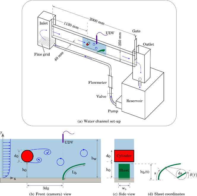
Figure 1: Schematic view of (a) the $2$-meter long water channel along with (b) top and (c) front view showing how the cylindrical obstacle is set-up in order to impose a vortex street forcing on a flexible sheet downstream.

All experiments are performed in a long-narrow water channel as schematized in Figure 1 (a). Water from the pump ($700$ – $2800$ lit/h) passes through a fine grid in the inlet and flows out in to a narrow $2$-meter long channel of width $4$ cm and height $25$ cm. By properly adjusting the outlet gate and the horizontal slope of the channel, it is possible to maintain a free-surface flow of uniform water height across the entire channel. At a little more than $1$-meter, a circular cylinder of diameter $d_{0}$ is fixed with its axis parallel to the floor, but perpendicular to the flow. Behind the cylinder (downstream), a thin flexible rectangular sheet is fixed firmly to the channel bottom. The sheet’s foot is fixed at a distance $3d_{0}$ from the cylinder’s center so that a well-developed vortex street is set-up Roshko (1954); Szepessy and Bearman (1992) in front of the sheet while the latter does not influence the cylinder’s wake flow. Finally, to avoid the effect of free-surface on the Vortex-Forced-Oscillations (VfO) of the sheet, and also for the sake of simplicity, the cylinder’s vertical location is taken as $h_{0}$ equal to the sheet height in a steady, uniform channel flow whose water height is kept identical throughout this work ($h_{w}=22.1$ cm). Figures 1 (b) – (c) illustrate this set-up wherein the cylinder and the sheet are exposed to an uniform channel flow directly orthogonal to the sheet’s section $L_{b}w_{b}$.

In the range of depth-averaged flow speed $U_{0}=2.2$ – $8.8$ cm s^-1 and diameters $d_{0}=10$, $20$, $40$ mm used here, the cylinder Reynolds number $Re_{d}=U_{0}d_{0}/\nu$ varies over a decade, between $236$ and $3773$. An Ultrasonic Doppler Velocimetry (UDV) is used to obtain vortex street characteristics at the center plane of the channel and at a fixed position downstream, equal to $3$ times the cylinder diameter. The probe measures the instantaneous vertical velocity component in the water flow at an acquisition frequency of about $2$ MHz during $3$ minutes. The range of shedding frequency varies between $0.14$ and $2.13$ Hz as indicated in the Table 1 (see also, Supplementary Material).

$d_{0}$	$U_{0}d_{0}/\nu$	$f_{v}$	$f_{v}/f_{n}$
(mm)		(Hz)
$10$	$236$ – $943$	$0.14$ – $0.63$	$2$ – $360$
$20$	$472$ – $1886$	$0.28$ – $1.26$	$1$ – $210$
$40$	$943$ – $3773$	$0.37$ – $2.13$	$0.8$ – $105$

Table 1: Characteristics of Bénard-Kàrmàn vortices for a range of water speed $U_{0}=2.2$ – $8.8$ cm s^-1. The shedding frequency were obtained using Ultrasonic Doppler Velocimetry (UDV). As compared to the cylinder Reynolds number $Re_{d}=U_{0}d_{0}/\nu$, the hydraulic Reynolds number $Re_{h}=U_{0}D_{h}/\nu$ varies from $1730$ to $6920$, wherein the hydraulic diameter is $D_{h}={4h_{w}w_{c}}/{(2h_{w}+w_{c})}$ and the water height $h_{w}=22.1$ cm is kept constant for all experiments. The reduced frequency $u=f_{v}/f_{n}\gtrsim 1$ for all cases considered here and also, it increases almost as $C_{y}^{9/5}$ (not shown here).

Five different cases of low-density polyethylene (density $\rho_{b}=920$ kg m^-3 and mass ratio $0.93$) sheets from GoodFellow Cambridge Limited are used in our experiments. A snap-off blade knife was used to cut large sheets to prepare long blades. This is a delicate task especially for longer and thinner sheets, as the process often leads to some local plastic deformation at its edges. In addition, some defects were initially present in the sheets. See Table 2 for the sheet length $L_{b}$, the thickness $e_{b}$ and other physical properties. The sheet thickness is chosen to be always very small compared to all other dimensions. For the sake of simplicity, the gap between the sheet and the channel walls is taken to be narrow, so that the force exerted by the channel flow on the sheet is predominantly due to profile drag. The Cauchy number

$$C_{y}=\dfrac{C_{d}\dfrac{1}{2}\rho U_{0}^{2}}{E}\left(\dfrac{L_{b}^{3}w_{b}}{I}\right),$$ (1)

which expresses the ratio of the flow drag and the elastic restoring forces, is varied in wide a range between $\mathcal{O}(1)$ and $10^{5}$. Here, $U_{0}$ is the depth-averaged flow speed, $E$ is the Young’s modulus, the second moment of inertia for a thin flexible sheet is taken as $I=w_{b}e_{b}^{3}/12$, and $C_{d}$ is the profile drag coefficient of a thin flat plate perpendicular to the flow direction. Based on measurements from our previous work, namely, Barsu et al. (2016, see fig. $6$a), $C_{d}=6$ is taken throughout the present work.

An estimate for the natural frequency of a fixed-free cantilever beam in a fluid can be found in classical texts such as Blevins (2015); Sumer and Fredsøe (2006):

$$f_{ni}=a_{i}\sqrt{\dfrac{EI/w_{b}L_{b}^{4}}{\rho_{b}e_{b}+{\pi C_{M}\rho w_{b}}/{4}}},$$ (2)

where $a_{i}$ is a non-dimensional constant with ($a_{1}=0.56$ and $a_{2}=3.5$ for the first-order and second-order natural frequency, resp.) and $C_{M}$ is the added mass coefficient. Note that this natural frequency is usually attributed to beams in fluids that undergo small-amplitude vibrations and small deflections. Hence, such a frequency might not be relevant to long flexible sheets considered in this study since they exhibit large deflections. Also, these sheets are pre-tensioned due to the presence of a mean flow drag.

ID	$L_{b}$	$e_{b}$	$E$	$C_{y}=\dfrac{C_{d}\frac{1}{2}\rho U^{2}}{E}\left(\frac{L_{b}^{3}w_{b}}{I}\right)$	$B_{a}=\dfrac{\Delta\rho ge_{b}}{E}\left(\frac{L_{b}^{3}w_{b}}{I}\right)$	$f_{n1}$	Symbol
	(mm)	(mm)	($\times 10^{6}$ Pa)			(Hz)
$S442$	$84$	$0.19$	$210$	$5$ – $88$	$0.55$	$0.286$	$\triangleleft$
$S1263$	$240$	$0.19$	$210$	$130$ – $2000$	$12.8$	$0.035$	$\Box$
$S1400$	$84$	$0.06$	$230$	$908$ – $4200$	$8.3$	$0.042$	$\bigcirc$
$S2000$	$200$	$0.10$	$250$	$2100$ – $9800$	$32.1$	$0.018$	$\medwhitestar$
$S4000$	$240$	$0.06$	$230$	$12500$ – $98200$	$192.4$	$0.005$	$\Diamond$

Table 2: Geometric and mechanical properties of low-density polyethylene sheets along with the range of related Cauchy numbers attained in this work. All sheets are less denser than water (density $\rho_{b}=920$ kg m^-3) and their width ($w_{b}=15$ mm) is kept constant throughout this work. The sheet ID also indicates their stiffness ratio given by $L_{b}/e_{b}$.

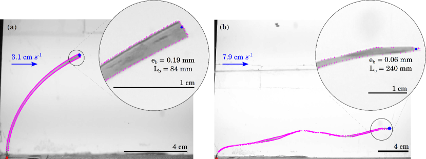
Figure 2: Two examples showing the results of sheet edge detection via ImageJ with insets displaying a zoom on the tip of the sheet. (a) S$442$: $C_{y}=11.3$, $Re_{h}=2.5\times 10^{3}$, $Re_{d}=1.4\times 10^{3}$ and (b) S$4000$: $C_{y}=7.83\times 10^{4}$, $Re_{h}=6.2\times 10^{3}$, $Re_{d}=3.4\times 10^{3}$. Here, dots (pink) show the detected sheet edge while an asterisk (blue) and a cross (red) each indicate the sheet’s tip and foot, respectively.

A high-resolution, full-frame digital camera (Sony $\alpha 7$) is used to image the Vortex-forced-Oscillations (VfO) of the flexible sheet at a rate of $25$ images per second for a time period of $7$ to $8$ minutes (see supplementary videos). The resulting images are analysed using the open-source freeware ImageJ Schindelin et al. (2012) and algorithms therein for brigthness thresholding Kapur et al. (1985); Tsai (1985), edge detection, etc. Sample images and the corresponding edge detection (dots, pink) are shown in figures 2(a) and (b). Clearly, the contour of the sheet is well-detected. The sheet “tip” is taken as the center of the last identified sheet edge. This allows for a well-resolved tip detection amplitudes in the order of a few $10$-th of a millimetre.

In the following sections, all experimental results are presented in terms of the depth-averaged water speed across the time-averaged deflected sheet height $\bar{h}_{b}$. This speed is based on the classical Coles law for the channel velocity profile $U(y)$, so that $U_{h}\bar{h}_{b}=\int_{0}^{\bar{h}_{b}}U(y)dy$. Each symbols, namely, $\triangleleft$, $\Box$, $\bigcirc$, $\medwhitestar$, and $\Diamond$, represent different sheets of increasing stiffness ratio ($L_{b}/e_{b}$), respectively, provided in Table 2.

III Time-averaged sheet reconfiguration

In the absence of a vortex street, at any chosen flow rate and constant water height, a sheet bends in the flow direction and exhibits a deflected height $h_{b}<L_{b}$. This leads to the well-known drag reduction since the profile drag force experienced by a flexible sheet $F_{d}=C_{d}\frac{1}{2}\rho U^{2}h_{b}w_{b}$ is smaller than that experienced by the same sheet, if it was rigid (here, $C_{d}$ is the sheet drag coefficient). Such a drag reduction is often quantified by expressing the so-called static reconfiguration number $\mathcal{R}=h_{b}/L_{b}$ as a function of the flow speed $U_{0}$ and the so-called Vogel number  Vogel (1989) i.e, $h_{b}/L_{b}\sim U_{0}^{\mathcal{V}}$. Thereby, the profile drag can be written as a power law

$$F_{d}\propto\dfrac{1}{2}\rho U_{0}^{2+\mathcal{V}}A_{f},$$

where $A_{f}=L_{b}w_{b}$ is the undeformed sheet frontal area. Then, drag reduction by reconfiguration is observed if the Vogel number is $\mathcal{V}<0$. For example, the Vogel number $\mathcal{V}=-2/3$ for long thin blades which are anchored to the flow bed at its one end de Langre (2008). While the reconfiguration number expresses the frontal area reduction, a more appropriate way to estimate drag reduction by reconfiguration is to compute the effective blade length proposed by (Luhar and Nepf, 2011). Such a length also includes the streamlining effect due to bending at the foot of the sheet. For the sake of simplicity, we consider the reconfiguration number which accounts only area reduction. This provides an upper bound for drag reduction by reconfiguration as well Luhar and Nepf (2011).

In this context, Figure 3 displays the dynamic reconfiguration number $\bar{\mathcal{R}}={\bar{h}_{b}}/{L_{b}}$ against water speed for each of the five sheets in our study. Here, each column correspond to data for a particular cylinder diameter $d_{0}$. Reconfiguration data in the absence of any upstream cylinder is also presented in each figure for comparison (open symbols; light magenta). We observe that the average reconfiguration number is always lesser than unity and the related time-averaged sheet deflection can be as small as one-tenth of its length. Furthermore, in all cases corresponding to a fixed $L_{b}/e_{b}$, $\bar{\mathcal{R}}$ decreases when the flow speed increases. So, the frontal area of a given sheet that is exposed to the incoming flow decreases with speed, leading to an average drag-reduction by reconfiguration. By comparing each filled symbol in Figure 3 with its corresponding open symbol, we note that $\bar{\mathcal{R}}={\bar{h}_{b}}/{L_{b}}$ always falls above the values of ${\mathcal{R}_{0}}={{h}_{0}}/{L_{b}}$. So, the time-averaged sheet-deflection at a given speed is systematically bigger than its counter-part in the case of a flexible sheet free of an upstream cylinder. We refer to this as a “lift-up” effect. It is observed to be more pronounced for bigger cylinder $d_{0}$ and also, at higher water speeds $U_{h}$. However, at a fixed $d_{0}$ and $U_{h}$, the influence of sheet’s stiffness ratio $L_{b}/e_{b}$ on the “lift-up” effect is not straight-forward.

Direct measurement of drag force is not possible in our experimental set-up. However, a measure of the average drag-reduction during the vortex-forced-motion of thin flexible sheets can be inferred from Figure 3 by estimating the so-called Vogel number $\mathcal{V}$. As it is common for the case of a steady flow over a flexible sheet, we associate a power law $\bar{h}_{b}/L_{b}\sim U_{h}^{\mathcal{V}}$ and deduce a Vogel number $\mathcal{V}$ for each stiffness ratio ($L_{b}/e_{b}$). Except for the sheet with the smallest stiffness, all the other sheets present a Vogel number $\mathcal{V}\approx-0.6\pm 0.1$. Note that similar values were previously obtained in the same water channel, but for submerged artificial canopies of kevlar sheets undergoing static reconfiguration (Barsu et al., 2016, , fig $4$(a)). We observe that the Vogel parameter is almost independent of cylinder diameter $d_{0}$ for sheets S$442$, S$1263$ and S$1400$. For more flexible blades (S$2000$ and S$4000$), a decrease in the Vogel parameter with increasing $d_{0}$ is observed. This suggests that vortices perhaps hinder the time-averaged drag reduction by reconfiguration of flow-bent flexible structures. In addition, this effect seems to be stronger for more flexible blades and bigger vortices.

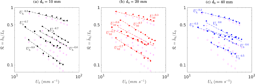
Figure 3: Time-averaged sheet reconfiguration $\bar{\mathcal{R}}_{b}=\bar{h}_{b}/L_{b}$ in the presence of Bénard-Kàrmàn vortices as a function of the depth-averaged water speed across the sheet height ($U_{h}$). All symbols indicate different stiffness ratio ($L_{b}/e_{b}$) as given in Table II. Open symbols represent data for the same cases as filled symbols but in the absence of an upstream cylinder.

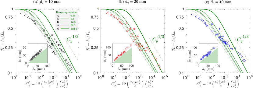
Figure 4: Time-averaged sheet reconfiguration $\bar{\mathcal{R}}_{b}=\bar{h}_{b}/L_{b}$ expressed in terms of the local Cauchy number $C_{y}^{h}=12\left({C_{d}\frac{1}{2}\rho U_{h}^{2}}/{E}\right)\left({L_{b}^{3}}/{e_{b}^{3}}\right)$ and compared with continuous lines (green) as obtained from the bending beam model (eqn. 4). The inset compares the average sheet deflection against the corresponding cylinder’s vertical position.

It is now well-established that a bending beam, accounting for the local flow drag and the Archimedes force due to buoyancy provides a satisfactory mechanical model for static reconfiguration of flexible sheets Alben et al. (2002); Luhar and Nepf (2011); Barsu et al. (2016); Leclercq and de Langre (2016). If $s$ is the curvilinear coordinate along the sheet and $\theta(s)$ the local sheet deflection as represented in fig. 1 (d), the restoring bending moment $\mathrm{M}(s)$ at any arbitrary distance $s$ from the sheet’s foot should be given by

$${{EI}\dfrac{d\theta}{ds}}=\int_{s}^{L_{b}}{\left(x(\xi)-x(s)\right)}dF_{\mathrm{A}}-\int_{s}^{L_{b}}{\left(\xi-s\right)}dF_{\mathrm{D}},$$ (3)

where $dF_{\mathrm{A}}=\Delta\rho g\left(e_{b}w_{b}d\xi\right)$ is the local Archimedes force and $dF_{\mathrm{D}}=C_{d}\frac{1}{2}\rho U^{2}\sin^{2}{\left(\theta(\xi)\right)}dA_{f}$ is the normal component of the local profile drag, with $\Delta\rho=\rho-\rho_{b}$ the density difference between the fluid and the sheet, and $dA_{f}=w_{b}d\xi$ the local frontal area of the reconfigured sheet. The above equation can be further simplified by taking both $U(s)\equiv U_{0}$ and $EI$ to be invariant across the sheet so that

$$\dfrac{d^{3}\theta}{d\tilde{s}^{3}}=B_{a}\left(\sin\theta\left(1-\tilde{s}\right)\dfrac{d\theta}{d\tilde{s}}+\cos\theta\right)-C_{y}\sin^{2}\theta,$$ (4)

where $\tilde{s}=s/L_{b}\in\left[0,1\right]$ is the non-dimensional curvilinear coordinate, $B_{a}=\Delta\rho gw_{b}e_{b}L_{b}^{3}/EI$ is the so-called Buoyancy number and $\mathcal{C}_{y}=C_{d}\rho w_{b}L_{b}^{3}{U}^{2}_{0}/2EI$ is the Cauchy number. The typical values for these non-dimensional numbers are also provided in Table 2. This model equation can be readily solved by applying the boundary conditions at the sheet extremities $\theta=\pi/2$ and $d\theta/ds=d^{2}\theta/ds^{2}=0$, for $\tilde{s}=0$ and $\tilde{s}=1$, respectively.

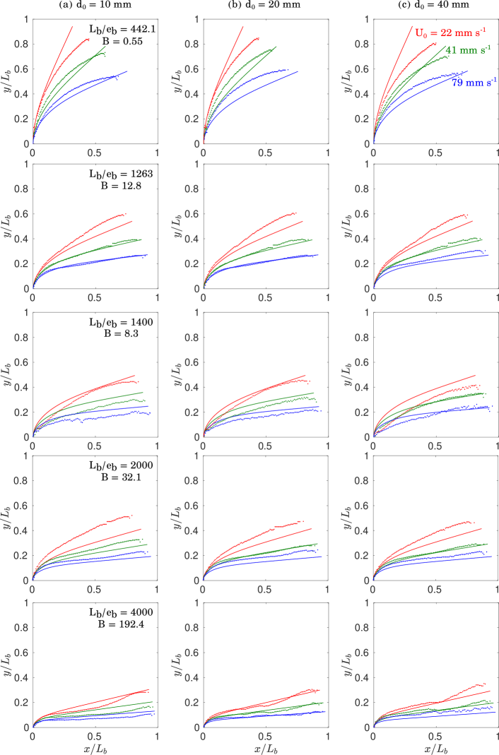
Figure 5: Typical time-averaged sheet shape from experiments (dots) as compared to bending beam model (continuous lines), allowing for the effect of buoyancy in a steady, uniform channel flow (eqn. 4).

Let us now investigate the dynamic reconfiguration number as a function of Cauchy number, as provided in Figure 4. As before, we use the depth-averaged water speed $U_{h}$ across the time-averaged deflected sheet height $\bar{h}_{b}$ to express data in terms of the local Cauchy number $C_{y}^{h}=12{C_{d}\frac{1}{2}\rho U_{h}^{2}}/{E}\left(L_{b}/e_{b}\right)^{3}$. Symbols represent experiments and continuous lines are computed from the bending beam model in eqn. (4) at each various Cauchy and Buoyancy number. For a given blade, say for instance S$442$ as represented by $\triangleleft$, as $C_{y}$ increases, the sheet reconfiguration decreases monotonically. However, at a fixed Cauchy number $C_{y}$, reconfiguration data from all sheets do not collapse on a single master curve. A closer observation reveals that this is due to buoyancy which tends to increase the reconfiguration for sheets of larger Buoyancy number $B_{a}=12{\Delta\rho ge_{b}}/{E}\left({L_{b}}/{e_{b}}\right)^{3}$. Despite the fact that the above-mentioned bending beam model is only valid for the case of a static reconfiguration under a steady uniform flow, it predicts the trend with the Cauchy number and also, the buoyancy number for all cases. It displays a reasonable agreement for $C_{y}>\mathcal{O}(1)$.

Furthermore, figure 5 compares the time-averaged sheet shape with that computed via the bending beam model (eqn. 4). Note that the model provides a satisfactory estimate despite the strong approximations such as uniform, steady flow across the sheet. As already mentioned in Section II, defects were often present in the biaxially oriented thin polyethylene sheets. This is visible for the most flexible blade in our study, namely, S$4000$ at the smallest speed ($U_{0}=22$ mm s^-1, red color). Nevertheless, the influence of non-uniform velocity profile is perhaps more significant on discrepancies between the model and the experiments than any initial plastic deformation.

Finally, an estimation for these differences between experimental data and the steady flow model can be obtained by analysing the “lift-up” effect. As observed in Figure 3 and Figure 4 (insets), the sheet deflection height $h_{b}/L_{b}$ in the absence of vortices is smaller than the dynamic reconfiguration $\bar{\mathcal{R}}=\bar{h}_{b}/L_{b}$. Also, the “lift-up” effect is more pronounced as the diameter of the upstream cylinder increases. And it arises from the presence of an upstream cylinder which leads to an oscillating velocity field in the vicinity of the sheet’s tip, and a velocity defect in the longitudinal component of the mean flow downstream. So, for some average velocity defect $\bar{\delta u}<0$, we deduce an estimate from the well-established power law ${h}_{0}/L_{b}\sim U_{h}^{\mathcal{V}}$ for static reconfiguration to obtain for its dynamic counter-part as $\bar{h}_{b}\sim h_{0}\left(1+\mathcal{V}\bar{\delta u}_{v}/U_{h}\right)$. Suppose that this defect occurs in the sheet tip’s neighbourhood of size $l_{v}$. Since the cylinder’s vertical position is fixed at $h_{0}$ for each experiment, we then have $\bar{\delta u}\sim-U_{h}l_{v}/h_{0}$, upto a first-order correction of the mean flow $U_{h}$. Therefore, it is expected that $\bar{h}_{b}\sim h_{0}-\mathcal{V}l_{v}$, with $\mathcal{V}<0$. Let us now compare this relationship with plots of $\bar{h}_{b}$ against $h_{0}$, as given in the insets of Figure 4. We note that the general trend of data points reasonably agrees with the relation $\bar{h}_{b}\sim h_{0}-\mathcal{V}l_{v}$. Hence, the “lift-up” effect in dynamic reconfiguration could be understood as a consequence of the presence of cylinder wake. It can also be inferred that the lengthscale $l_{v}$ depends on the cylinder diameter $d_{0}$. Nonetheless, the decrease in the Vogel exponent for more flexible sheets can not be completely explained via a small-velocity defect argument as here. This phenomenon is perhaps analogous to time-averaged reconfiguration in wave-induced oscillations of submerged flexible structures Luhar and Nepf (2016); Lei and Nepf (2019a); Lei and Nepf (2019b). They obtain a scaling law for both the effective blade length Luhar and Nepf (2011) and the deflected height is found to be $\bar{h}_{b}/L_{b}\sim C_{y}^{-1/4}$ with a proportionality constant which depends on the ratio of the blade length and the wave amplitude. Thus, our results suggest that the dynamic reconfiguration tends towards to wave-induced mean blade reconfiguration when the cylinder diameter increases.

IV Sheet oscillation amplitude

If $({x}_{b}(t),{y}_{b}(t))$ represent sheet tip’s instantaneous position and $(\bar{x}_{b},\bar{y}_{b})$ their time-average, then let us define the tip oscillation amplitude based on the standard deviation as in

$$\delta_{b}\equiv 2\sqrt{\overline{\left(x_{b}(t)-\bar{x}_{b}\right)^{2}}+\overline{\left(y_{b}(t)-\bar{y}_{b}\right)^{2}}},$$ (5)

where $\bar{\cdot}$ represents mean values. Figure 6 presents such an amplitude as a function of the local water speed $U_{h0}=U(y=h_{0})$ computed from the Coles law channel velocity profile times the cylinder diameter $d_{0}$. Also, $U_{h0}d_{0}$ is proportional to the local cylinder Reynolds number. Each open symbol corresponds to a stiffness ratio as given in Table 2 and other symbols $\cdot$, $+$ and $\times$ indicate cylinder diameters $d_{0}=10$, $20$ and $40$ mm, respectively. For a given sheet and cylinder, the tip fluctuation amplitude increases proportionally with the local water speed $U_{h0}$. Now, as the cylinder diameter is varied similar behaviors are again observed but the tip amplitudes $\delta_{b}$ are smaller for smaller diameters. In addition, sheets with higher stiffness ratio $L_{b}/e_{b}$ show increasingly larger amplitudes while data for sheets with approximatively same stiffness ratio, as in S$1263$ ($\Box$) and S$1400$ ($\bigcirc$) fall almost on the same linear trend line. In general, it is inferred from these observations that the tip amplitude not only increases with the sheet stiffness ratio $L_{b}/e_{b}$, but also with $U_{h0}d_{0}$.

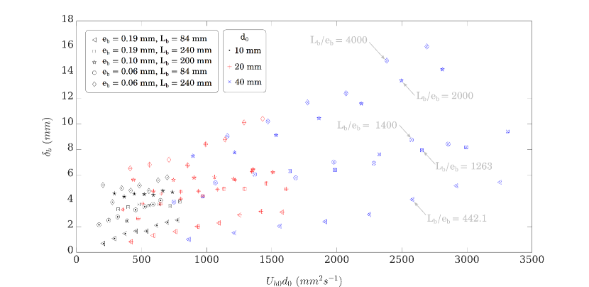
Figure 6: Tip oscillation amplitude $\delta_{b}$ as a function of an equivalent vortex circulation $U_{h0}d_{0}$, where $U_{h0}$ is the water speed at the cylinder center.

A simple model can be derived if we decompose the total work done by the vortex-laden flow on the flexible sheet into two distinct parts : $(i)$ the steady component of the flow leads to the average angular position, say $\bar{\xi}$, and $(ii)$ the periodic interaction between the vortices and spring-supported flat plate results in torsional vibrations of the spring, and hence the plate’s angular position $\xi(t)$. Then, locally, the average profile drag-induced moment should be balanced by the average restoring moment in the deflected sheet $EI{d\theta}/{ds}$, where ${d\theta}/{ds}$ is the sheet’s local curvature ($1/R_{c}$). As already observed in section III, at very large Cauchy number which compares drag force against the elastic restoring force, $\bar{h}_{b}\ll L_{b}$ and hence, it can be safely assumed that $EI{d\theta}/{ds}\approx{EI}/{\bar{h}_{b}}$, since $R_{c}$ is approximately equal to the time-averaged sheet deflection $\bar{h}_{b}$ (see Figure 7). And so, we obtain

$$\dfrac{EI}{\bar{h}_{b}} \sim \left(C_{d}\dfrac{1}{2}\rho U_{0}^{2}w_{b}\bar{h}_{b}\right)\times\bar{h}_{b},$$ (6)

$$\Rightarrow\dfrac{\bar{h}_{b}}{L_{b}} \sim C_{y}^{-1/3},$$

a result analogous to the well-known scaling for the static reconfiguration number de Langre (2008); Gosselin (2019) that leads to drag reduction in flexible plates. When $C_{y}\ll 1$, on the other hand, ${\bar{h}_{b}}\approx{L_{b}}$. Note that the experimental data provided in the previous section, as in Figure 3, match fairly well with the above large-Cauchy number scaling law, irrespective of Buoyancy number. In general, the above result could also be expressed as ${\bar{h}_{b}}/{L_{b}}\sim C_{y}^{\mathcal{V}/2}$, where the Vogel number $\mathcal{V}=-2/3$ at $C_{y}\gg 1$ de Langre (2008).

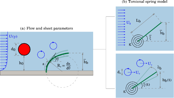
Figure 7: Schematic of the flow and sheet parameters along with that of the torsional spring model.

Furthermore, we propose that the vibrational energy of the sheet is solely taken from Bénard-Kàrmàn vortices at some rate depending on the characteristics of the incoming unsteady flow, and during some time scale proportional to the shedding period $1/f_{v}$. Therefore, for the toy-model, we have

$$\dfrac{1}{2}\mathcal{K}\left(\dfrac{\delta_{b}}{L_{b}}\right)^{2}\sim\left(\dfrac{1}{2}\rho U_{0}^{3}w_{b}d_{v}\right)\dfrac{1}{f_{v}},$$ (7)

where the left-hand-side is the vibrational energy of the torsional spring and the right-hand-side is the product of local kinetic energy transfer rate, taken here as proportional to $1/2\rho U_{0}^{3}w_{b}d_{v}$, and the typical timescale during which the transfer periodically takes place, i.e., $1/f_{v}$. Here, $d_{v}$ is some characteristic lengthscale of Bénard-Karman vortices. Also, in the above expression, the stiffness $\mathcal{K}$ of the pre-tensioned torsional spring can be ascertained from the equilibrium condition that $\mathcal{K}\bar{\xi}\equiv EI{d\theta}/{ds}\approx{EI}/{\bar{h}_{b}}$, with $\bar{\xi}\approx{\bar{h}_{b}}/{L_{b}}$ when $Ca\gg 1$ since ${\bar{h}_{b}}\ll{L_{b}}$. Now, in terms of the Vogel number $\mathcal{V}=-2/3$ at $C_{y}\gg 1$, or $\mathcal{V}=0$ at $C_{y}\ll 1$. By admitting that the dynamic reconfiguration number is $\bar{h}_{b}/{L_{b}}\sim C_{y}^{\mathcal{V}/2}$, it can be deduced that $\mathcal{K}\sim\left({EI}/L_{b}\right)C_{y}^{-\mathcal{V}}$. Thereafter, the expression 7 leads to

$$\left(\dfrac{\delta_{b}}{L_{b}}\right)^{2} \sim \left(\dfrac{\rho U_{0}^{2}w_{b}L_{b}}{EI}\right)\left(\dfrac{U_{0}d_{v}}{f_{v}}\right)C_{y}^{\mathcal{V}},$$ (8)

$$\Rightarrow\dfrac{\delta_{b}}{d_{v}} \sim C_{y}^{n}{St_{v}}^{-1/2},$$ (9)

where $St_{v}=f_{v}d_{v}/U_{0}$ is the Strouhal number based on a typical size of the eddies, and $n\equiv\left(1+\mathcal{V}\right)/2=1/6$, or respectively $1/2$, for sufficiently large Cauchy numbers $C_{y}\gg 1$, or otherwise.

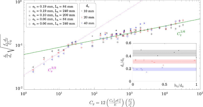
Figure 8: All data from Figure 6 are expressed in terms of the rescaled oscillation amplitude of the sheet’s free-end $\delta_{b}/d_{0}$ as given by the relationship 9 versus the Cauchy number $C_{y}=12\left({C_{d}\frac{1}{2}\rho U_{0}^{2}}/{E}\right)\left({L_{b}^{3}}/{e_{b}^{3}}\right)$. Two distinct regimes are visible here.

Figure 8 presents the same tip amplitude data given in Figure 6 but instead, they are rescaled in terms of the experimentally obtained values of the Strouhal number $St_{h}$, cylinder centreline velocity $U_{h0}$ and the characteristic vortex length scale $d_{v}$ (see supplementary material and also, inset Figure 8). Clearly, experimental data ranging over all Cauchy numbers investigated here are regrouped around two distinct trend lines, namely $C_{y}^{1/2}$ and $C_{y}^{1/6}$, each corresponding to the case of moderately small and large Cauchy numbers, respectively, as expressed by the relation 9. In the former, the sheet reconfiguration is sufficiently small and so, it represents vibration of a rigid sheet forced by a vortex street. Whereas, in the latter case, sheets can be considered to be flexible. These results strongly suggest that the torsional spring model contains the essential mechanism to explain the observed vortex-forced-vibration of thin sheets. They also imply that, analogous to drag-reduction via reconfiguration under an external flow, a flexible sheet experiences a smaller vibration amplitude compared to that of a rigid sheet when excited by a Bénard-Kàrmàn vortex street. Finally, it is pointed out that the expression the dynamic reconfiguration number may not in general be given by $\bar{h}_{b}/{L_{b}}\sim C_{y}^{\mathcal{V}/2}$ and this expression is valid only for either sufficiently small, or large, Cauchy numbers Gosselin et al. (2010). In addition, the reconfiguration number should also depend on the Buoyancy number for intermediate Cauchy numbers Luhar and Nepf (2011). So, it is possible that the transition between the two regimes of vortex-forced-oscillations may perhaps not be as abrupt as in our experiments.

V Sheet beating frequency

The time evolution of tip response of a sheet S$442$ subject to Bénard-Kàrmàn vortices shed by a cylinder ($d_{0}=40$ mm) at the lowest and highest water speed is considered in this section. , respectively are displayed in Figures 9(a) & (b). In Figures 9(a) , at $U_{0}=3.1$ cm s^-1, both vertical and horizontal oscillations are of the same order of magnitude and also, they are synchronous. As the speed increases to $U_{0}=7.9$ cm s^-1, $y$-fluctuations present an almost proportionally-increased back-and-forth amplitude while $x$-fluctuations are much smaller in magnitude. Clearly, $x$-tip detection seems to be not so robust for this case. Their corresponding power spectral density are provided on the immediate right of the same figures. Here, arrows are used to indicate the forcing frequency (vortex shedding) $f_{v}=0.56$ Hz and the first natural frequency $f_{n1}=0.29$ Hz, respectively. Clearly, the sheet tip oscillates at the vortex shedding frequency for these two cases.

The above examples correspond to the sheet for which the relevant Cauchy numbers ($C_{y}=5$ – $88$) are the smallest. In comparison, Figure 9(c) gives the tip fluctuations for S$4000$, at one of the largest Cauchy numbers ($C_{y}=9\times 10^{4}$). This sheet exhibits large amplitude oscillations in the vertical direction as big as the cylinder diameter $d_{0}=40$ mm while the horizontal oscillations remain small ($\lesssim 4$ mm) as before. The corresponding spectra of vertical tip position presents a peak at $0.15$ Hz, along with a smaller second peak at the vortex shedding frequency $f_{v}=0.55$ Hz. Qualitatively similar temporal characteristics are observed for the sheet tip when the diameter $d_{0}$ is decreased. For example, Figure 9(d) provides a typical data at $d_{0}=10$ mm to be compared with its equivalent case at the same water speed and sheet physical properties given in Figure 9(c). Firstly, the vertical oscillations are diminished almost in proportions to the diameter-ratio. Secondly, the power spectral density presents a peak neither at the vortex shedding frequency $f_{v}=0.55$ Hz, nor at the sheet natural frequency $f_{v}=5\times 10^{-3}$ Hz. Instead, the peak occurs at almost the same frequency ($0.16$ Hz $<f_{v}$) as for the case with the larger diameter $d_{0}=40$ mm. In fact, this peak is much closer to the flat-plate shedding frequency based on the average-deflected-height of the sheet, i.e, $0.145U_{h}/\bar{h}_{b}=0.2$ for these cases. In summary, the peak-normalised power spectra suggests that the tip motion in the $y$ direction oscillates either at the vortex shedding frequency $f_{v}$ or at a different frequency lesser than $f_{v}$ as and when $d_{0}$ decreases, or $L_{b}/e_{b}$ increases.

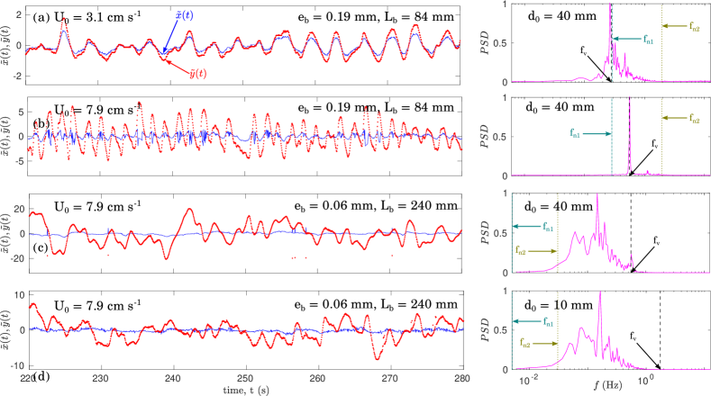
Figure 9: [Left] Blade tip oscillations (in mm) of the “stiffest” sheet S$442$ at different depth-averaged water speed (a) $U_{0}=3.1$ cm s^-1, (b) $U_{0}=7.9$ cm s^-1 as compared with the “most flexible” sheet S$4000$ at (c) $U_{0}=7.9$ cm s^-1 due to vortices shed by a cylinder of diameter $d_{0}=40$ mm. (d) Same as (c) but for $d_{0}=10$ mm. [Right] Power spectral density of the sheet tip’s vertical fluctuations. Arrows indicate various frequencies, namely, the vortex-shedding frequency ($f_{v}$) and the first two sheet natural frequencies ($f_{n1}$ and $f_{n2}$).

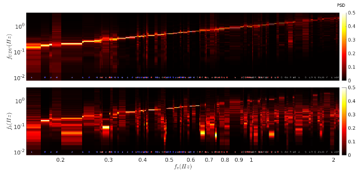
Figure 10: Power spectral density for all experimental cases as a function of the forcing frequency $f_{v}$, corresponding to imposed periodic shedding of Bénard-Kàrmàn vortices. The frequency content of the [TOP] vertical velocity behind the cylinder, as measured using an UDV and [BOTTOM] vertical fluctuations of the sheet’s free-end. Dashed line is given simply to show the trend while symbols are provided for the sake of reference only (see Figure 8, for the corresponding sheet physical properties).

Figure 10 (TOP) displays a color plot of the power spectral density of the UDV-measured, instantaneous vertical velocity at the cylinder mid-span and at a distance $3d_{0}$ downstream the cylinder wake. As already mentioned, UDV measurements were acquired at $2$ MHz during $3$ minutes. Colors, from bright yellow to black, represent the normalised spectra of the $y$-component velocity field across the cylinder diameter. Here, the spectra at each $y$-coordinate ($y\in[h_{0},h_{0}+d_{0}]$) is first computed and then an average in the discrete Fourier space is taken to obtain the normalised spectra. The latter presents a maximum (bright yellow, in Figure 10 (TOP)) at a frequency $f$ which is, by definition, equal to the vortex shedding frequency $f_{v}$.

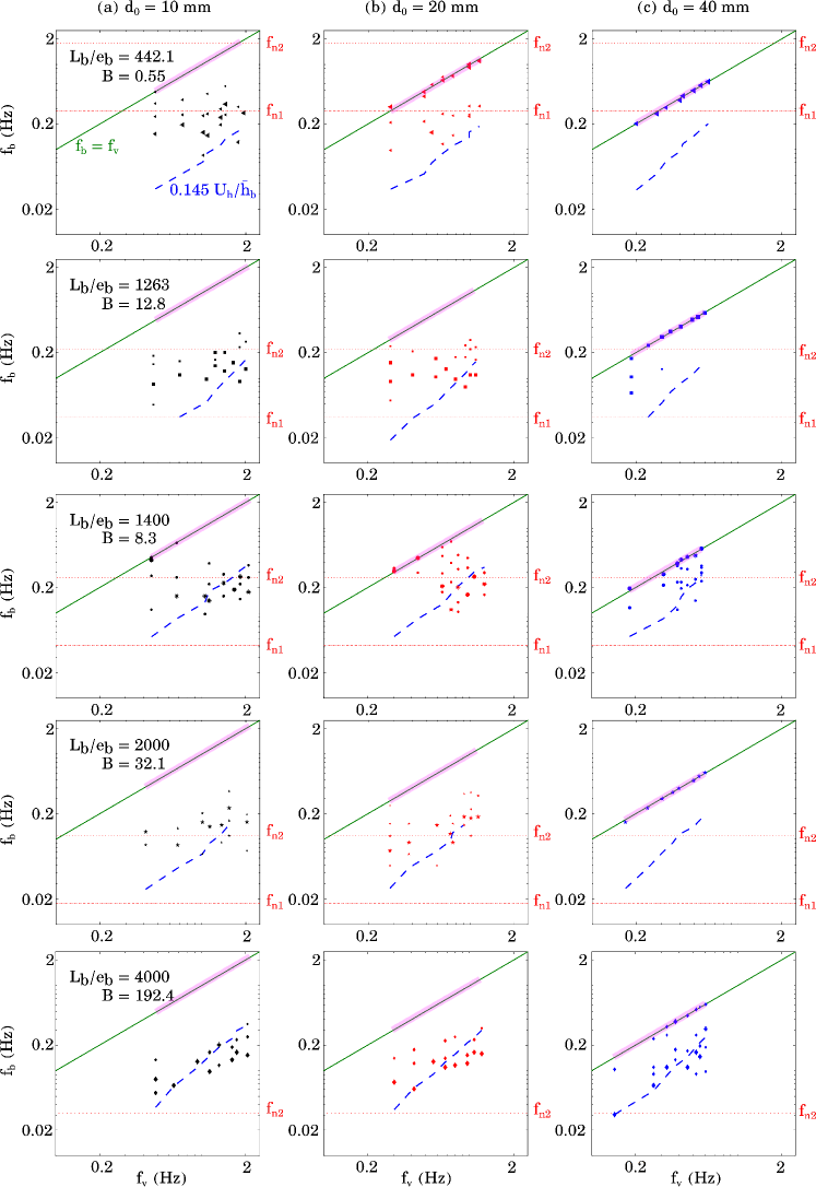
Figure 11: A detailed view of the measured blade peak frequency as a function of the vortex shedding frequency $f_{v}$. Symbols denote the same cases as in Figure 6 while symbol size at each forcing frequency $f_{v}$ is proportional to the normalized power spectral density. Here, the continuous line (——) represents $f_{b}=f_{v}$ while the dot-dash line (${\color[rgb]{1,0,0}-\cdot-}$) and the dotted line (${\color[rgb]{1,0,0}\cdots}$) indicate the sheet’s first and second natural frequency $f_{n1}$ and $f_{n2}$, respectively, and (${\color[rgb]{0,0,1}---}$) is the flat-plate shedding frequency based on the sheet deflected height $f_{h}=0.145U_{h}/\bar{h}_{b}$. Also, in each case, pink bands indicate the forcing frequency range.

Similarly, Figure 10 (BOTTOM) presents the power spectral density for the sheet-tip $y_{b}(t)$. For the sake of comparison, the $x$-axis is kept the same as just before. Therefore, this figure illustrates the energy content of the sheet-tip oscillation for each forcing frequency, equal to the shedding frequency of the Bénard-Kàrmàn vortices $f_{v}$. Note that the sheet tip position spectra is not quite the same as the $y$-component velocity power spectra discussed just before. Clearly, there are many cases where the power spectrum is wide for a fixed $f_{v}$. It is thereby inferred that the sheet’s vibrational energy is distributed across different frequencies and the dominant frequency $f_{b}$ varies from case to case. Nonetheless, the dominant frequency of sheet tip fluctuations is observed, in general, to be lower than the vortex shedding frequency $f_{v}$. Also, a second peak is often visible for some cases in Figure 10 (BOTTOM).

To further elucidate the distribution of vibrational energy in the sheet-tip vertical motion, Figure 11 provides a few dominant tip frequencies $f_{b}$, i.e., those frequencies corresponding to the prominent peaks in the corresponding power spectral density, for various imposed vortex shedding frequency. Size of the data points are proportional to the normalized power spectra. In this figure, data in each row corresponds to a single sheet characteristics, in the ascending order of the sheet stiffness ratio $L_{b}/e_{b}$ while each column denotes data from experiments with the same cylinder diameter $d_{0}$. The cylinder diameter $d_{0}$ increases from left to right. Here, the continuous line (green) provided to indicate the cases when $f_{b}=f_{v}$, i.e., the cases where the observed beating frequency of the sheet is equal to the forcing frequency due to Bénard-Kàrmàn vortices. Now it can be inferred from the data displayed in the last column, for experiments with the largest cylinder ($d_{0}=40$ mm), that the dominant frequency in the sheet-tip fluctuations is simply equal to the forcing frequency $f_{v}$, irrespective of the Cauchy number $C_{y}=12\left({C_{d}\frac{1}{2}\rho U^{2}}/{E}\right)\left({L_{b}^{3}}/{e_{b}^{3}}\right)$. This is in contrast with the case when $d_{0}=10$ mm wherein $f_{b}<f_{v}$ for all sheets and multiple prominent peaks in the power spectra of the tip’s vertical fluctuation $\tilde{y}_{b}(t)$. However, for some case, namely, S$442$ and S$1263$, the prominent frequencies are about the first, or second natural sheet frequency, respectively, as given by eqn. (2). Whereas, for the other cases, the data is scatter around the dashed-line (blue) which denotes the expression $f_{h}=0.145U_{0}/\bar{h}_{b}$, the flat-plate shedding frequency Blevins (1977) based on the sheet deflected height $\bar{h}_{b}$, as known from the dynamic sheet reconfiguration. We also observe similar dynamical regimes for the intermediate cylinder size $d_{0}=20$ mm : (i) For the most rigid sheet S$442$ and for $C_{y}<20$, the dominant blade frequency is seen to be the forcing frequency $f_{v}$, with a few dominant peaks either at the sheet’s first natural frequency $f_{n1}$, (ii) For the most flexible sheets, namely, S$2000$ and S$4000$ and for $C_{y}>10^{3}$ the sheets display oscillations at the vortex shedding frequency of an inclined flat plate given by $f_{h}=0.145U_{0}/\bar{h}_{b}$, and (iii) For moderate stiffness ratio and Cauchy numbers, the sheet oscillates either at one of its natural frequency which is close to the forcing frequency $f_{v}$ or at the inclined plate shedding frequency $f_{h}$. Finally, it is pointed out here that no conclusive evidence for a critical Cauchy number, nor a critical length scale for the vortices, is observed in these data. Nonetheless these observations strongly suggest that, in general, there is a transition from the forced-vortex-synchronous sheet-tip oscillation regime ($f_{b}=f_{v}$) to either a regime wherein the sheet-tip oscillations resemble the classical lock-in mode or a regime wherein the tip vibrations are induced by its wake characteristics. And the transition between these dynamical oscillation modes should depend on the relative size of the Bénard-Kàrmàn vortices and the stiffness ratio.

VI Conclusions

The role of vortical structures in a transverse water flow on the flow-induced reconfiguration and vibration of a thin flexible sheet fixed to the floor at one end are experimentally investigated. Sheets of varying lengths and thicknesses ($L_{b}=84$ – $240$ mm; $e_{b}=0.06$ – $0.19$ mm) and three different cylinder diameters $d_{0}=10$, $20$ and $40$ mm are used for this purpose. Each experiment consist of rigidly anchoring the sheet to the channel bottom and then systematically exciting its free-end by vortices shed by a cylinder upstream. The forcing frequency is $f_{v}=0.14$–$2.1$ $Hz$ for different depth-averaged water speed $U_{0}=22$ – $88$ mm s^-1, so that the cylinder Reynolds number varies between $Re_{d}\equiv\rho U_{0}d_{0}/\mu=240$ – $3800$.

Our experiments show that the time-averaged reconfiguration of a thin sheet follows qualitatively the same scaling with the Cauchy number $C_{y}=12\left({C_{d}\frac{1}{2}\rho U_{0}^{2}}/{E}\right)\left({L_{b}^{3}}/{e_{b}^{3}}\right)$ as in the case of a thin sheet in an uniform, steady flow bends, so that its time-averaged profile drag is reduced. A simple bending beam model for steady flow which takes into account the drag force, and also the buoyancy force, as in Luhar and Nepf (2011), provides a reasonably good match with observations, if the flow speed $U_{0}$ is replaced by that of a local speed based on depth-averaged steady velocity profile given by Coles law Coles (1956). This suggests that the average drag force $\bar{F}_{d}=C_{d}1/2\rho U_{0}^{2}\bar{h}_{b}w_{b}\propto U_{0}^{2+\mathcal{V}}$. Here, $\bar{h}_{b}\propto L_{b}U_{0}^{\mathcal{V}}$ is the time-averaged sheet deflection and $\mathcal{V}<0$ for drag reduction is the so-called Vogel number and it is observed to be $\mathcal{V}\approx-0.6\pm 0.1$ in the present work. The influence of vortices is nonetheless visible for bigger cylinder diameters where there exists a slight “lift-up” effect leading to a small decrease in the sheet reconfiguration and Vogel exponent. This is attributed to the average velocity defect in the cylinder wake so that the mean sheet deflection is given by $\bar{h}_{b}\sim h_{0}-\mathcal{V}l_{v}$, where $h_{0}$ is the deflection in the absence of vortices and $l_{v}$ is a characteristic lengthscale of the wake in the vicinity of the sheet tip.

For a given blade thickness ($e_{b}$) and length ($l_{b}$), the oscillation amplitude ($\delta_{b}$) of the sheet tip increases with the Reynolds number $Re_{d}$. It is also demonstrated that the Cauchy number is the appropriate parameter to scale all data in terms of the non-dimensional amplitude $\delta_{b}/d_{0}$. The underlying mechanism that controls sheet-tip oscillations is then analyzed via a toy-model which consists of torsional spring-mounted rigid flat plate subject to an external flow which is decomposed into a uniform steady flow and a regular array of vortices. If the former is taken to control the average sheet reconfiguration and the latter is assumed to provide the necessary work for the forced vibration the sheet. It is then shown that the rescaled oscillation amplitude $\delta_{b}/d_{v}\sim C_{y}^{(1+\mathcal{V})/2}St_{v}^{-1/2}$, where $d_{v}$ is the typical lengthscale of the vortex core and $St_{v}=f_{v}d_{v}/U_{0}$ the related Strouhal number. In particular, for a relatively rigid sheet wherein the average drag force provides only a very little sheet deflection i.e., $\mathcal{V}\approx 0$, $\delta_{b}/d_{0}\sim C_{y}^{1/2}$. This corresponds to the cases where the Cauchy number is either small, or at most moderate. Also, in this case, the sheet vibrates like a rigid curved plate as its local curvature does not change sign over the sheet’s entire length. On the other hand, at large Cauchy number $C_{y}>10^{2}$, for a relatively flexible sheet wherein the average drag force results in a strong sheet reconfiguration i.e., when $\mathcal{V}\approx-2/3$ de Langre (2008), the non-dimensional vibration amplitude of the sheet free-end $\delta_{b}/d_{0}\sim C_{y}^{1/6}$. Note that, in the second regime, sheet exhibits modal oscillations like a flapping flag wherein transverse waves which travel forward towards the sheet free-end appear (see supplemental videos).

In regards to the beating frequency ($f_{b}$) of the sheet free-end, three dynamical regimes are observed in this study: (i) Tip oscillations follow the forcing frequency $f_{v}$ corresponding to vortex shedding from the upstream cylinder, (ii) Tip oscillation frequency is related to vortex shedding behind a free inclined rigid plate of frontal height equal to the average sheet deflection $\bar{h}_{b}$ such that $f_{b}\sim 0.145U_{h}/\bar{h}_{b}$, and (iii) Sheet vibrations occur at one of its natural frequency $f_{n}$, near the forcing frequency. When the cylinder diameter $d_{0}=40$ mm, sheet tip oscillates at the forcing frequency $f_{v}$, irrespective of the Cauchy number studied here ($C_{y}<10^{5}$). For smaller cylinders, the sheet displays flow-induced vibration controlled by its wake characteristics as in (ii) or a lock-in motion at its natural frequency as in (iii). Furthermore, this transition is possibly dependent on the average sheet reconfiguration and sheet thickness as well.

In a classical textbook by Blevins (1977), many investigations on Flow-Induced-Vibration are classified into two general categories depending on the incoming flow, namely, a steady or an unsteady flow. Our work is a sub-category of the latter case wherein we provide a case study for interactions between eddies and a flexible sheet. Indeed, more work is necessary to understand and hence predict the above-mentioned dynamical regimes via flow visualization, PIV measurements of the flow around the sheet and in its wake. The potential effect of sheet confinement is also left for future investigations.

References

- Roshko (1954) A. Roshko (1954).
- Roshko (1961) A. Roshko, Journal of fluid mechanics 10, 345 (1961).
- Berger and Wille (1972) E. Berger and R. Wille, Annual Review of Fluid Mechanics 4, 313 (1972).
- Williamson (1996) C. H. Williamson, Annual review of fluid mechanics 28, 477 (1996).
- Sarpkaya (1979) T. Sarpkaya, ASME Journal of Applied Mechanics 46, 241 (1979).
- Bearman (1984) P. W. Bearman, Annual review of fluid mechanics 16, 195 (1984).
- Sarpkaya (1995) T. Sarpkaya, ASME Journal of Offshore Mechanics and Arctic Engineering 117 (1995).
- Sarpkaya (2004) T. Sarpkaya, Journal of fluids and structures 19, 389 (2004).
- Williamson and Govardhan (2004) C. H. Williamson and R. Govardhan, Annu. Rev. Fluid Mech. 36, 413 (2004).
- Bearman (2011) P. Bearman, Journal of Fluids and Structures 27, 648 (2011).
- Blevins (1977) R. D. Blevins, Flow-induced vibration (Van Nostrand Reinhold Co., New York, 1977), ISBN 0-442-20828-6.
- Paidoussis (1998) M. P. Paidoussis, Fluid-structure interactions: slender structures and axial flow, vol. 1 (Academic press, 1998).
- Sumer and Fredsøe (2006) B. M. Sumer and J. Fredsøe, Hydrodynamics around cylindrical structures (revised edition), vol. 26 (World Scientific, 2006).
- Naudascher and Rockwell (2017) E. Naudascher and D. Rockwell, Flow-induced vibrations: an engineering guide (Routledge, 2017).
- Koehl (1984) M. Koehl, American Zoologist 24, 57 (1984).
- Vogel (1984) S. Vogel, American Zoologist 24, 37 (1984).
- Vogel (1989) S. Vogel, Journal of Experimental Botany 40, 941 (1989).
- Koehl (1996) M. Koehl, Annual Review of Ecology and Systematics 27, 501 (1996).
- Vogel (1994) S. Vogel, Life in moving fluids: the physical biology of flow (Princeton University Press, 1994).
- de Langre (2008) E. de Langre, Annual Review of Fluid Mechanics 40, 141 (2008), ISSN 0066-4189.
- Gosselin (2019) F. P. Gosselin, Journal of Experimental Botany 70, 3533 (2019).
- Leclerc and de Langre (2018) T. Leclerc and E. de Langre, Journal of Fluid Mechanics 838, 606 (2018).
- Shelley and Zhang (2011) M. J. Shelley and J. Zhang, Annual Review of Fluid Mechanics 43, 449 (2011).
- Siniscalchi and Nikora (2013) F. Siniscalchi and V. Nikora, Journal of hydraulic research 51, 46 (2013).
- Jin et al. (2018a) Y. Jin, J. Kim, and L. P. Chamorro, Physical Review Fluids 3, 044701 (2018a).
- Jin et al. (2018b) Y. Jin, J.-T. Kim, L. Hong, and L. P. Chamorro, Physics of Fluids 30, 097102 (2018b).
- Jin et al. (2018c) Y. Jin, J.-T. Kim, Z. Mao, and L. Chamorro, Journal of Fluid Mechanics 852 (2018c).
- Jin et al. (2019) Y. Jin, J. Kim, S. Fu, and L. P. Chamorro, Journal of Fluid Mechanics 864, 273 (2019).
- Nepf (2012) H. M. Nepf, Annual Review Fluid Mechanics 42, 44 (2012).
- Gosselin and de Langre (2009) F. P. Gosselin and E. de Langre, European journal of Mechanics B/Fluids 28, 271 (2009).
- Finnigan (1979) J. Finnigan, Boundary-Layer Meteorology 16, 181 (1979).
- Py et al. (2006) C. Py, E. de Langre, and B. Moulia, Journal of Fluid Mechanics 568, 425 (2006).
- Ackerman and Okubo (1993) J. Ackerman and A. Okubo, Functional Ecology pp. 305–309 (1993).
- Ghisalberti and Nepf (2002) M. Ghisalberti and H. M. Nepf, Journal of Geophysical Research 107 (2002).
- Singh et al. (2016) R. Singh, M. M. Bandi, A. Mahadevan, and S. Mandre, Journal of Fluid Mechanics 786 (2016).
- Tschisgale et al. (2021) S. Tschisgale, B. Löhrer, R. Meller, and J. Fröhlich, Journal of Fluid Mechanics 916 (2021).
- Nikora et al. (2012) V. Nikora, S. Cameron, I. Albayrak, O. Miler, N. Nikora, F. Siniscalchi, M. Stewart, M. O’HARE, W. Rodi, and M. Uhlmannm, Environmental Fluid Mechanics: Memorial Volume in Honour of Professor Gerhard H. Jirka’. IAHR Monographs.(Eds W. Rodi and M. Uhlmann.) Chapter 11 (2012).
- Jin et al. (2016) Y. Jin, S. Ji, and L. P. Chamorro, Physical Review E 94, 063105 (2016).
- Barsu (2016) S. Barsu, Ph.D. thesis, Université Claude Bernard Lyon (2016).
- Szepessy and Bearman (1992) S. Szepessy and P. Bearman, Journal of Fluid Mechanics 234, 191 (1992).
- Barsu et al. (2016) S. Barsu, D. Doppler, J. John Soundar Jerome, N. Riviere, and M. Lance, Physics of Fluids 28 (2016).
- Blevins (2015) R. D. Blevins, Formulas for dynamics, acoustics and vibration (John Wiley & Sons, 2015).
- Schindelin et al. (2012) J. Schindelin, I. Arganda-Carreras, E. Frise, V. Kaynig, M. Longair, T. Pietzsch, S. Preibisch, C. Rueden, S. Saalfeld, B. Schmid, et al., Nature methods 9, 676 (2012).
- Kapur et al. (1985) J. Kapur, P. Sahoo, and A. Wong, Computer Vision, Graphics, and Image Processing 29, 273 (1985), ISSN 0734-189X.
- Tsai (1985) W.-H. Tsai, Computer Vision, Graphics, and Image Processing 29, 377 (1985), ISSN 0734-189X.
- Luhar and Nepf (2011) M. Luhar and H. M. Nepf, Limnology and Oceanography 56, 2003 (2011), ISSN 00243590.
- Alben et al. (2002) S. Alben, M. Shelley, and J. Zhang, Nature 420, 479 (2002).
- Leclercq and de Langre (2016) T. Leclercq and E. de Langre, Journal of Fluids and Structures 60, 114 (2016).
- Luhar and Nepf (2016) M. Luhar and H. M. Nepf, Journal of Fluids and Structures 61, 20 (2016).
- Lei and Nepf (2019a) J. Lei and H. M. Nepf, Coastal Engineering 147, 138 (2019a), ISSN 0378-3839.
- Lei and Nepf (2019b) J. Lei and H. M. Nepf, Journal of Fluids and Structures 87, 137 (2019b), ISSN 0889-9746.
- Gosselin et al. (2010) F. Gosselin, E. De Langre, and B. A. Machado-Almeida, Journal of Fluid Mechanics 650, 319 (2010).
- Coles (1956) D. Coles, Journal of Fluid Mechanics 1, 191 (1956).