QuTE: decentralized multiple testing on sensor networks with false discovery rate control

Abstract

This paper designs methods for decentralized multiple hypothesis testing on graphs that are equipped with provable guarantees on the false discovery rate (FDR). We consider the setting where distinct agents reside on the nodes of an undirected graph, and each agent possesses p-values corresponding to one or more hypotheses local to its node. Each agent must individually decide whether to reject one or more of its local hypotheses by only communicating with its neighbors, with the joint aim that the global FDR over the entire graph must be controlled at a predefined level. We propose a simple decentralized family of Query-Test-Exchange (QuTE) algorithms and prove that they can control FDR under independence or positive dependence of the p-values. Our algorithm reduces to the Benjamini-Hochberg (BH) algorithm when after graph-diameter rounds of communication, and to the Bonferroni procedure when no communication has occurred or the graph is empty. To avoid communicating real-valued p-values, we develop a quantized BH procedure, and extend it to a quantized QuTE procedure. QuTE works seamlessly in streaming data settings, where anytime-valid p-values may be continually updated at each node. Last, QuTE is robust to arbitrary dropping of packets, or a graph that changes at every step, making it particularly suitable to mobile sensor networks involving drones or other multi-agent systems. We study the power of our procedure using a simulation suite of different levels of connectivity and communication on a variety of graph structures, and also provide an illustrative real-world example.

1 Introduction

Research on decentralized detection and hypothesis testing has a long history, dating back to seminal work from the 1980s (e.g., [25, 24]), and with more recent work motivated in particular by wireless sensor networks (e.g., [6, 1, 16, 26, 4]). A variety of issues have been addressed, including robustness [11], quantization error [13], the sequential nature of data collection [10], battery/energy management of the sensors [23], tolerance of misbehaving nodes [22], nonparametric methods [12, 15], and bandwidth constraints [14]. However, these have focused on the ability to make a decision about a single global hypothesis in a distributed fashion. In contrast, this paper studies the testing of multiple hypotheses in a decentralized manner.

To be more specific, consider a graph with one agent at each node, and suppose that each agent wishes to test one or more binary hypotheses that are local to its node, with each hypothesis corresponding to the presence or absence of some signal. Of this collection of hypotheses, an unknown subset corresponds to true null hypotheses (absence of signal), whereas the rest are false (presence of signal), and should be rejected. Apart from having access to the data and hypotheses at its own node, each agent may also directly communicate with neighboring nodes on the graph. Our setup is directly related to, yet complementary to, the works of [9, 20, 27, 19].

For explicit context, one example of such an agent could be a low-power sensor with the ability to perform local measurements and simple computations. Then, the graph may represent a multitude of such sensors deployed over a widespread area, such as a forest, building or aircraft. Due to power constraints, the agent may communicate locally with agents at neighboring nodes, but only infrequently communicate with a distant centralized server. A rejected hypothesis corresponds to a discovery of some sort, such as a detected anomaly or a deviation from expected or recent measurements, and it is only in such cases that a local node is allowed to communicate with the central server.

Each agent aims to test their local null hypotheses, and reject a subset of nulls, proclaiming them to be false based on its local neighborhood information. We assume that each agent can calculate a $p$-value for each of its local hypotheses, which provides evidence against the respective null. This paper is agnostic to the exact methods that the node uses to calculate its local $p$-values; this topic has received significant attention in past work, and can be done in various ways. Each agent must use the local $p$-values, and possibly those of its neighbors, to decide which hypotheses to reject locally. The challenge is that these local decisions must be made with the aim of controlling a global error metric. In this paper, the error metric is chosen as the overall false discovery rate (FDR) across the whole graph, and we require that the FDR must be controlled at a pre-defined level.

The false discovery rate (FDR) is an error metric that generalizes the notion of type-1 error, or false positive error, to the setting of multiple hypotheses. It is defined as the expected ratio of the number of false discoveries to the total number of discoveries. It was first proposed by Eklund [7], and various heuristic methods were discussed by Eklund and Seeger [8, 21]. Its contemporary usage has been popularized by the seminal paper of Benjamini and Hochberg [2] who rigorously analyzed a procedure that is now known as the Benjamini-Hochberg (BH) procedure.

Algorithms to control the FDR make sense in settings where type-1 errors are possibly more costly than type-2 errors. Since such an asymmetry arises naturally in many situations, the FDR has nevertheless become one of the de-facto standard error metrics employed across a wide range of applied scientific fields. Its most common application is in a batched, centralized setting, where all the $p$-values are pooled, and a decision is made by thresholding them at some data-dependent level, such as the level determined by the Benjamini-Hochberg (BH) procedure [2].

In this paper, we develop a novel family of algorithms for decentralized FDR control on undirected graphs. Both the setting and the family of algorithms are new, to the best of our knowledge. Building on recent theoretical advances, we prove that global FDR over the whole graph is controlled under two types of dependence assumptions between the $p$-values at the different nodes; the setting of independent $p$-values is easiest, but a general type of “positive dependence” termed PRDS can also be handled.

A given instantiation of the QuTE algorithm is simple and scalable, and works as follows. First, a node queries its neighbors for their $p$-values. Second, it conducts a local test on the local neighborhood $p$-values at an appropriate level determined by the ratio of the size of its neighborhood to the size of the graph. Third, if a node thinks that neighboring hypotheses should be rejected, it informs the relevant neighbors. Lastly, each node rejects one or more of its local hypotheses as long as either its local test suggested so, or if any of its neighbors suggested so. We run simulations on a variety of graphs, including Erdös-Rényi random graphs and planar grid graphs, to provide some intuition about their achieved FDR and power. We also give an illustrative example of possible real-world applications of our setup and algorithm using a public Intel Lab dataset involving low-power sensors taking various kinds of measurements in a large open space.

Beyond guarantees on FDR control, our family of QuTE algorithms has another appealing property. When the graph is either complete (contains all edges) or a star, there exists at least one node that can access all the information in the network, in which case our algorithms reduce to the batch Benjamini-Hochberg procedure. When the graph is empty (without edges), and each node tests only one hypothesis without information about other nodes in the network, then our algorithms essentially reduce to the conservative Bonferroni procedure. Hence, one can view our algorithm as bridging the two extremes, depending on how much information is available at each node.

The rest of this paper is organized as follows. Section 2 presents the problem setup, including definitions and assumptions. We formally describe our algorithms and their associated theoretical guarantees in Section 3. We present the proof of our main theorem in Appendix A and Appendix B. We run a variety of simulations in Section 4 and illustrate an application to real data in Section 5. A discussion of our work and future directions can be found in Section LABEL:sec:disc.

2 Background and problem setup

Consider a graph $G=(\mathcal{V},\mathcal{E})$, where each node $a\in\mathcal{V}$ is associated with an agent. A given agent $a$ may communicate directly with any of its neighbors $b$, meaning nodes for which the edge $(a,b)$ belongs to the edge set. Associated with agent $a$ is a collection $\mathcal{H}_{a}=\{H_{a,i}\}_{i=1}^{n_{a}}$ of $n_{a}$ hypotheses to be tested. The sum $N=\sum_{a\in\mathcal{V}}n_{a}$ corresponds to the the total number of hypotheses. Out of these, let $\mathcal{H}^{0}_{a}$ represent the (unknown) subset of true null hypotheses at node $a$, and let $\mathcal{H}^{0}=\cup_{a\in\mathcal{V}}\mathcal{H}^{0}_{a}$ represent the overall set of true null hypotheses. We assume that the agent at each node observes one $p$-value corresponding to each hypothesis at that node, labeled $P_{a,1},\dots,P_{a,n_{a}}$. It is understood that when a null hypothesis is true, the corresponding $p$-value is stochastically larger than the uniform distribution (super-uniform, for short), meaning that

$$\text{ for all $H_{a,i}\in\mathcal{H}^{0}$, we have }\textnormal{Pr}\!\left\{{P_{a,i}\leq u}\right\}\leq u\text{ ~{} for all $u\in[0,1]$}.$$ (1)

Given observations of the $p$-values at its node, each agent may communicate with its neighbors, and must then decide which subset of its hypotheses to reject; each rejection is called a discovery, and rejecting a true null hypothesis corresponds to a false discovery. Let $R$ be the total number of discoveries, and $V$ be the total number of false discoveries. Even though each agent makes a local decision with only local information, we might still desire to control a global measure of error. However, even in the centralized setting, there is no single notion of type-1 error for multiple testing problems; we discuss two common variants below.

2.1 False Discovery Rate (FDR)

One classical quantity is the family-wise error rate (FWER), which is defined as $\textnormal{Pr}\!\left\{{V>0}\right\}$. A procedure that guarantees that $\text{FWER}\leq\alpha$ might be desirable in applications where a false discovery is extremely costly, and must be avoided at all costs. One simple way to control the FWER is the Bonferroni procedure, which rejects every $p$-value that is smaller than $\alpha/N$; the FWER guarantee follows by an application of the union bound.

However, in many practical settings involving even a moderately large number $N$ of hypotheses, the FWER metric is too stringent and the associated procedures (like Bonferroni and its variants) have very low power, making very few discoveries for a given level of FWER control. This issue led Eklund [7], in collaboration with Seeger [8], and more recently Benjamini and Hochberg [2] to propose an alternative notion of error, called the false discovery rate (FDR), which we now define and adopt in this work. We adopt the convenient notation $\mathchoice{\ooalign{$\genfrac{}{}{0.0pt}{0}{a}{b}$\cr\leavevmode\cleaders\hbox to2.20001pt{\hss$\displaystyle\cdot$\hss}\hfill\kern 0.0pt\cr}}{\ooalign{$\genfrac{}{}{0.0pt}{1}{a}{b}$\cr\leavevmode\cleaders\hbox to2.20001pt{\hss$\textstyle\cdot$\hss}\hfill\kern 0.0pt\cr}}{\ooalign{$\genfrac{}{}{0.0pt}{2}{a}{b}$\cr\leavevmode\cleaders\hbox to2.20001pt{\hss$\scriptstyle\cdot$\hss}\hfill\kern 0.0pt\cr}}{\ooalign{$\genfrac{}{}{0.0pt}{3}{a}{b}$\cr\leavevmode\cleaders\hbox to2.20001pt{\hss$\scriptscriptstyle\cdot$\hss}\hfill\kern 0.0pt\cr}}=\frac{a}{\max{b,1}}$, and define the false discovery rate (FDR) to be

$$\small\textnormal{FDR}=\mathbb{E}\left[{\mathchoice{\ooalign{$\genfrac{}{}{0.0pt}{0}{V}{R}$\cr\leavevmode\cleaders\hbox to1.98001pt{\hss$\displaystyle\cdot$\hss}\hfill\kern 0.0pt\cr}}{\ooalign{$\genfrac{}{}{0.0pt}{1}{V}{R}$\cr\leavevmode\cleaders\hbox to1.98001pt{\hss$\textstyle\cdot$\hss}\hfill\kern 0.0pt\cr}}{\ooalign{$\genfrac{}{}{0.0pt}{2}{V}{R}$\cr\leavevmode\cleaders\hbox to1.98001pt{\hss$\scriptstyle\cdot$\hss}\hfill\kern 0.0pt\cr}}{\ooalign{$\genfrac{}{}{0.0pt}{3}{V}{R}$\cr\leavevmode\cleaders\hbox to1.98001pt{\hss$\scriptscriptstyle\cdot$\hss}\hfill\kern 0.0pt\cr}}}\right].$$

As suggested by the name, it corresponds to the expected proportion of false discoveries relative to the total number of discoveries. On average, a procedure with FDR controlled at level $\alpha$ will return a collection of discoveries of which at most an $\alpha$-fraction are false.

2.2 Centralized algorithms for FDR control

All existing algorithms for FDR control have been designed for the centralized setting, where a single agent has access to all $N$ $p$-values. In such a setting, if $P_{(j)}$ is the $j$-th smallest $p$-value, then the Benjamini-Hochberg (BH) algorithm [2] rejects the hypotheses corresponding to the smallest $\widehat{k}$ $p$-values $P_{(1)},\dots,P_{(\widehat{k})}$, where $\widehat{k}$ is a data-dependent integer chosen by the rule

$$\widehat{k}^{BH}=\max\big{\{}k\mid P_{(k)}\leq\alpha\frac{k}{N}\big{\}}.$$

This procedure guarantees that the FDR is controlled at level $\alpha$ when the $p$-values are independent [2]. Equivalently, the BH procedure rejects all $p$-values that are at most $\alpha\frac{\widehat{k}^{BH}}{N}$.

Benjamini and Yekutieli [3] proved that the BH algorithm also guarantees FDR control when the $p$-values satisfy a general notion of positive dependence called positive regression dependence on a subset (PRDS). Since our results also hold under this condition, we define it formally now.

For a pair of vectors $x,y\in[0,1]^{N}$, the notation $x\preceq y$ means that $x\leq y$ in the orthant ordering, i.e., $x_{j}\leq y_{j}$ for all $j\in\{1,\dots,N\}$. We say that a function $f:[0,1]^{N}\mapsto\mathbb{R}^{+}$ is nonincreasing, if $x\preceq y$ implies $f(x)\geq f(y)$. Similarly, we say that a subset $\mathcal{D}$ of $[0,1]^{n}$ is nondecreasing if $x\in\mathcal{D}$ implies $y\in\mathcal{D}$ for all $y\succeq x$.

Definition 1 (PRDS, positive dependence)

For any nondecreasing set $\mathcal{D}\subseteq[0,1]^{N}$ and $H_{a,j}\in\mathcal{H}^{0}$, the function $t~{}\mapsto~{}\textnormal{Pr}\!\left\{{P\in\mathcal{D}}\ \middle|\ {P_{a,j}\leq t}\right\}$ is nondecreasing on $(0,1]$.

The PRDS condition holds trivially if the $p$-values are independent, but also allows for some amount of “positive” dependence. Let us consider a simple example to provide some intuition. Let $Z=(Z_{1},\ldots,Z_{N})$ be a multivariate Gaussian vector with covariance matrix $\Sigma$; the null components correspond to Gaussian variables with zero mean. Letting $\Phi$ be the CDF of a standard Gaussian, the vector $P=(\Phi(Z_{1}),\dots,\Phi(Z_{N}))$ is PRDS (on every null index) if and only if all entries of the covariance matrix $\Sigma$ are non-negative. See the paper [3] for other examples of this type.

The BH algorithm has been extended to a variety of settings; see [17] for a survey. In this paper, we consider the new setting of decentralized multiple testing, for which there are no known algorithms or guarantees for FDR control.

2.3 Communication Protocol

In engineering applications such as low-power wireless sensor networks, often there is no central agent that has access to all $p$-values. Indeed, while it might be possible for each sensor to communicate with a central server, such communication could consume signficant power if the distances involved are large. It would make more sense for each sensor to communicate with a central server only if something anamolous is happening at or around that node, corresponding to a (rare) rejected hypothesis.

A reasonable model is that each agent can communicate only with its neighbors. In this work, we assume that noiseless real numbers (like $p$-values) can be transmitted without error or quantization. Except for possible communication between the agents, the problem we consider is static. This means that the graph structure, the hypotheses at each node, and their associated $p$-values, do not change with time. In other words, we consider a snapshot of network at one point in time, leaving extensions for future work.

Decentralized testing is, almost by definition, harder than centralized testing. Indeed, it should be intuitively clear that among all algorithms that guarantee FDR control, a centralized one will make more discoveries, because it has access to more information. Hence, the price that we will pay by restricting communication, while still demanding FDR control, will be in the achieved power of the algorithms, which is their ability to make true discoveries.

3 The QuTE Algorithm

For simplicity, we first describe a single-step Query-Test-Exchange (QuTE) algorithm. If more communication is feasible, then the extension to a multi-step QuTE algorithm is straightforward, and presented in a later subsection.

We assume that each node has a unique ID, and that the agent knows this ID. Each agent $a$ fixes an order of the hypotheses (and corresponding $p$-values) at its node, and forms a vector $\vec{P}_{a}$ with an ordered list of $p$-values at node $a$. The single-step QuTE algorithm proceeds as follows:

• Query: Each agent queries its neighbors for the vectors that they are in possession of. Each agent receives an ordered vector of $p$-values from every neighbor, and keeps track of which neighbor each $p$-value came from.

• Test: Let $S_{a}$ be the set $p$-values now in possession of agent $a$. Agent $a$ runs the BH procedure on its $|S_{a}|$ $p$-values, at an adjusted target FDR of $\alpha_{a}:=\alpha\frac{|S_{a}|}{N}$. Equivalently, agent $a$ assumes that all $p$-values it does not know equal 1, and runs the BH procedure on all $N$ $p$-values at level $\alpha$. Denoting the number of rejections at node $a$ by $\widehat{k}_{a}$, it is natural that these $\widehat{k}_{a}$ rejections may include some of agent $a$’s own hypotheses, and some from its neighbors.

• Exchange: All agents exchange their rejection decisions with their neighbors by sending back an ordered indicator vector, informing the neighbors to reject every hypothesis that has its indicator location set to unity.

At the end of a single pass of these three steps, each agent then rejects any hypothesis that it has been informed that it should reject. Hence, an agent rejects any local hypothesis rejected by its own test, or by the tests of any of its neighbors. This algorithm comes with the following guarantee.

Theorem 1

Suppose that $p$-values are independent or positively dependent. Then for any graph topology, the aforementioned QuTE algorithm achieves FDR control at level $\alpha\frac{|\mathcal{H}^{0}|}{N}$.

See Appendix A for the proof of Theorem 1. The algorithm is seemingly quite liberal with its rejections, in the sense that when determining whether a hypothesis should be rejected or not, each agent does not take a majority vote amongst its neighbors, but rejects whenever even a single neighbor thinks it should be rejected. Nevertheless, it still manages to guarantee FDR control on any graph.

3.1 Dependence on graph topology

Informally speaking, more edges in the graph results in better connectivity, more information per agent, and higher power. We can precisely characterize what the QuTE algorithm does on some special graph structures below:

• When the graph has no edges, and each agent has only one hypothesis, then QuTE reduces to the Bonferroni correction, where a hypothesis is rejected if and only if its $p$-value is at most $\alpha/N$.

• When there exists at least one node which is connected to all others, like in a star graph or a clique, then after the query step, this agent possesses all the $p$-values, and then QuTE reduces to the classical BH algorithm.

The price that one pays for limited information is power. We can make this somewhat precise, by introducing a partial ordering over graphs. For any two graphs on the same node set, we say that $G_{1}\sqsupset G_{2}$ whenever $E_{1}\supset E_{2}$. The relation $\sqsupset$ defines a partial ordering over such graphs. Fix the number of nodes, and also the hypotheses and $p$-values at every node, and let $\mathcal{R}(G)$ denote the set of rejections made by the QuTE algorithm on graph $G$, and let $R(G)=|\mathcal{R}(G)|$. We then have the following result.

Proposition 1

The number of rejections made by the QuTE algorithm is nondecreasing with respect to $\sqsupset$, meaning that conditioning on the observed $p$-values, we have

$$G_{1}\sqsupset G_{2}\implies\mathcal{R}(G_{1})\supseteq\mathcal{R}(G_{2}).$$

Remark: By taking absolute values, and then expectations over the randomness in $p$-values, we also conclude that $G_{1}\sqsupset G_{2}$ implies that $\mathbb{E}\left[{R(G_{1})}\right]\geq\mathbb{E}\left[{R(G_{2})}\right]$, meaning that the power of QuTE is also nondecreasing with respect to $\sqsupset$.

See Appendix B for the proof of Proposition 1. An immediate consequence of this proposition is that the power of QuTE can never exceed the power of BH. This is simply because the clique dominates all graphs with respect to $\sqsupset$, and QuTE reduces to BH on the clique. Some other effects of graph topology are explored in the simulations.

3.2 Extension to multi-step QuTE algorithms

The essential ingredient in the proof of Proposition 1 is the following fact: the more $p$-values to which a node has access, the more rejections its local test can make. This fact opens up the possibility of having $c>1$ rounds of querying before conducting the local test, followed by $c>1$ rounds of exchanging the results after testing. We call this the multi-step QuTE algorithm.

To be more explicit, multiple rounds of communication allow an agent to access the $p$-values at nodes that are not immediate neighbors. Indeed, with $c$ rounds of communication, it is straightforward that a node can access $p$-values of all nodes that are at a distance $\leq c$ away from it on the graph. After performing its local test, $c$ rounds of exchanging information can once again propagate the results of its local test to nodes that are at a distance $\leq c$ away.

Theorem 2

If the $p$-values are independent or positively dependent, then the multi-step QuTE algorithm with $c\geq 0$ rounds of communication guarantees that $\textnormal{FDR}\leq\alpha\frac{|\mathcal{H}^{0}|}{N}$.

The proof of Theorem 2 is very similar to the proof of Theorem 1, so we do not reproduce it. We can precisely characterize the QuTE algorithm at the two extremes of communication:

• When $c=0$ rounds of communication are allowed, and each agent has only one hypothesis, then QuTE reduces to the Bonferroni correction, where a hypothesis is rejected if and only if its $p$-value is at most $\alpha/N$.

• If $d$ is the diameter of the graph, then $\lceil d/2\rceil$ rounds of communication suffice for QuTE to achieve same power as a centralized BH procedure (and further communication makes no difference).

Note that the above stated bound is a worst-case upper bound on how much communication suffices, and one can often achieve the same power as a centralized algorithm with fewer than $\lceil d/2\rceil$ rounds.

4 Simulations

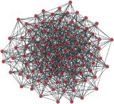
(a)

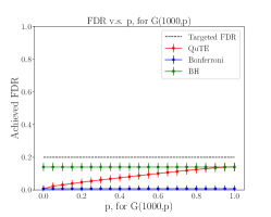
(b)

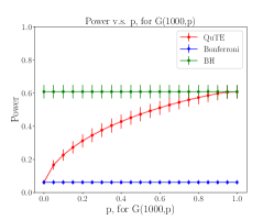
(c)

Figure 1: (a) Illustration of an Erdös-Rényi random graph $G(100,0.15)$. (b) Plot of FDR versus edge probability $p$. (c) Plot of power versus edge probability $p$. Panels (b) and (c) show results for the QuTE, BH and Bonferroni procedures applied to the random graph model $G(1000,p)$, with target FDR $\alpha=0.2$, signal level $\mu=2$ and the null-proportion $\pi_{0}=0.7$ .

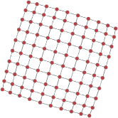
(a)

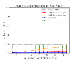
(b)

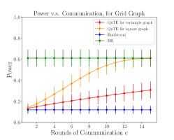
(c)

Figure 2: (a) Illustration of a $10\times 10$ grid graph. Panels (b) and (c) display FDR and power versus rounds of communcation on a $16\times 16$ grid graph and $2\times 128$ grid graph, for multi-step QuTE for a BH procedure, and Bonferroni procedure, with target FDR $\alpha=0.2$, signal level $\mu=2$ and the null proportion $\pi_{0}=0.7$.

We now examine the behavior of QuTE on two different types of graphs, Erdös-Rényi random graphs and grid graphs. In both settings, each node tests a single hypothesis, with a $p$-value independently generated from the following model:

$$\small X\sim\mu+\mathcal{N}(0,1);\text{ $p$-value }P=1-\Phi(X),$$ (2)

where $\Phi$ is the standard Gaussian CDF, with $\mu=0$ for nulls and $\mu>0$ for alternatives. In both experiments, we compare the performance of QuTE with the BH method and the Bonferroni correction, fixing the target FDR as $\alpha=0.2$, signal strength $\mu=2$ and null-proportion $\pi_{0}=\frac{|\mathcal{H}^{0}|}{N}=0.7$. Code for reproducing empirical results is available online.

4.1 Erdös-Rényi Random Graphs

We first study the effects of increasing edge density for Erdös-Rényi random graphs $G(N,p)$. In this model, an edge between any two distinct nodes is included in the graph with probability $p$ independently, as illustrated in Figure 1(a). In our experiments, we set $N=1000$, varying the edge probability $p$ from $0$ to $1$ in steps of $0.05$. We then randomly generate $1000$ $p$-values from model (2), each randomly assigned to one node of the graph.

Results are shown in panels (b) and (c) of Figure 1. We repeat our experiments $100$ times, and the error bars are taken to be the empirical standard deviations. One can observe that both the achieved FDR and power increase with the edge probability $p$. In particular, recall that QuTE reduces to Bonferroni when there is no edge ($p=0$) and reduces to BH test when the graph is complete ($p=1$).

4.2 Grid Graphs

We now study the effect of communication and graph structure on power, within the family of two-dimensional grids, that is, a planar graph whose vertices correspond to points with integer coordinates $(x,y)$, with $x=1,\dots,m$ and $y=1,\dots,n$. Edges exist between any two points with unit distance, as exemplified in Figure 2(a). Variants of such graphs may be encountered in environmental applications, where sensors are placed over a forest or lake. We consider a square grid with $m=n=16$ and a rectangular grid with $m=2,n=128$. In either case, $N=m\times n=256$ $p$-values are first randomly generated from model (2) and then randomly assigned to the nodes. We vary the number of the rounds of communication $c$ in multi-step QuTE on the two grids.

Results as the parameter $c$ varies are shown in Figure 2 (b, c). For each choice of $c$, we repeat the simulation $1000$ times, and the error bars are again taken to be the empirical standard deviations. In both grids, the achieved FDR and the power increase with the rounds of communication $c$. The square grid graph always achieves a higher FDR and power when $c$ is large, as each node can effectively get information from a larger number of nodes. Multi-step QuTE achieves comparable power as BH on the square grid graph when the number of the rounds of communication is close to $c=16$, when the center node can reach all of the nodes on the graph.

5 An Illustrative Example on Real Data

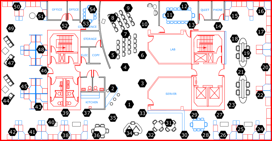
Figure 3: Arrangement of sensors in the lab [5].

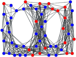
(a) Threshold $\gamma=0.1$

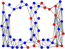
(b) Threshold $\gamma=0.3$

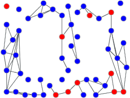
(c) Threshold $\gamma=0.5$

Figure 4: The three figures show the result of test at a common sample ($100$ epochs). The graphs are specified by choosing the threshold on communication probability to be $0.1,0.3,0.5$ for (a),(b),(c) respectively. The nodes in red are rejected.

We now provide an illustrative example for potential applications of QuTE to sensor networks. We use the publicly available Intel Lab dataset [5], which contains data collected from $54$ sensors deployed in the Intel Berkeley Research Lab. The distribution of sensors is shown in Figure 3. Mica2Dot sensors with weather boards collected timestamped topology information, along with humidity, temperature, light and voltage values once every $31$ seconds for $36$ days. Here, we only use the temperature measurement for simplicity, but note that our theory can handle the case when there are several hypotheses per node, possibly with positively dependent $p$-values. Each sensor can communicate with another sensor with certain probability, which is estimated by averaging connectivity data over time. This communication probability is provided in the dataset [5]. For simplicity, we threshold the probability and put an edge between two sensors if their communication probability with each other is larger than a threshold $\gamma\in\{0.1,0.3,0.5\}$.

Data preprocessing

The temperature data has a slowly increasing trend. We detrend the data for each sensor by first fitting a regression line and then subtracting the least squares fit. To reduce noise, we average over every consecutive $100$ epochs for each sensor to get a sample. That is, one sample has $54$ average temperature measurements from respective sensors within a consecutive $100$ epochs.

Hypotheses and $p$-values

At each node, the null hypothesis states that the current temperature at the node is normal over one randomly chosen time sample ($100$ epochs).

Define the empirical distribution of the temperature of the first $500$ samples at sensor $a$ as $\hat{F}_{n,a}$. Then we define the $p$-value at sensor $a$ as $P_{a}=2\min(1-\hat{F}_{n,a}(t_{a}),\hat{F}_{n,a}(t_{a})),$ where $t_{a}$ is the temperature of sensor $a$ in the current sample. We adopt the non-asymptotic calculation of $p$-values instead of using standard student t-tests because the empirical distribution has a heavy tail and is not asymptotically normal. In any case, this choice was made for illustration, and our method is agnostic to the exact method used to construct $p$-values, as long as they satisfy condition (1). As temperature measurements at the same time are positively correlated, the $p$-values are also positively correlated and we are justified in using QuTE to control FDR.

Results

The three subplots of Figure 4 display the results for three graphs formed by thresholding communication probabilities at $\gamma\in\{0.1,0.3,0.5\}$. The nodes in red are rejected, and naturally, there are more rejections on average with increasing density of edges. Given that QuTE provably controls the FDR under positive dependence, one can expect a large number of the rejected nodes to be true discoveries of an anomalous temperature at the current snapshot of time.

6 The quantized Benjamini-Hochberg and QuTE procedures

The aforementioned QuTE algorithm transmits real-valued $p$-values along the edges of the graph at each step. In practice, it is natural to avoid transmitting real-valued observations. Hence, we next introduce the notion of a $p$-rank which are integers between $1$ and $N$, and develop a “quantized BH” procedure that is written in terms of $p$-ranks instead of $p$-values, and makes the same decisions as the original one. This allows one to transmit integers using at most $\lceil\log(N)\rceil$ bits per $p$-rank.

We define the $p$-rank associated with a $p$-value $P_{i}$ as

$$\text{$p$-rank}_{i}=\min(\lceil P_{i}N/\alpha\rceil,N).$$

Since the BH procedure cannot reject $p$-values larger than $\alpha$, the truncation at $N$ does not matter for power. It is important to note that $p$-ranks are always integers between $1$ and $N$, and different $p$-values could be mapped to the same $p$-ranks, since

$$\text{$p$-rank}_{i}=s~{}\iff~{}(s-1)\alpha/N<P_{i}\leq s\alpha/N,$$

and there might be several $p$-values in the same range.

We define the quantized BH algorithm (or BH^Q for short), which works only with $p$-ranks, as follows. It first sorts the $p$-ranks, breaking ties arbitrarily. Calling the $i$-th sorted $p$-rank as $\text{$p$-rank}_{(i)}$, we define

$$\widehat{k}^{Q}:=\max\{k:\text{$p$-rank}_{(k)}\leq k\}.$$

Then BH^Q rejects the first $\widehat{k}^{Q}$ of the sorted hypotheses, meaning it rejects every hypothesis such that $\text{$p$-rank}_{(k)}\leq\widehat{k}^{Q}$.

The quantized QuTE procedure is defined analagously — in every Query and Exchange round, only quantized $p$-values are transmitted, and in each Test round, each node runs BH^Q at level $\alpha$ on its $p$-values (while assuming all unknown $p$-values equal 1). Then, we have the following result.

Theorem 3

The quantized BH procedure makes exactly the same discoveries as the BH procedure. As an immediate consequence, the quantize QuTE procedure makes exactly the same discoveries as the QuTE procedure.

A simple proof is provided in Appendix C.

7 Some extensions

Anytime-valid $p$-values for sequential QuTE.

For simplicity of notation, below we assume that each node is testing just one hypothesis (this is by no means a restriction, and the results go through seamlessly with multiple hypotheses per node).

The presented QuTE algorithm assumed that the $p$-values $P_{a}$ were fixed, and the only dynamism involved was to do with the communication protocol, where the passage of time only affected how much information each node knew about the rest of the graph. Here, we argue that QuTE can be easily extended to settings involving sequential testing, where data streams in over time, and hence the $p$-values $P_{a,t}$ change over time as more data is accumulated.

In the non-sequential setting, null $p$-values $P_{a}$ are constructed to be superuniform when the null hypothesis is true, as seen in condition (1). The natural generalization of this condition to the sequential setting is that the $p$-values $P_{a,t}$ are superuniform at any (possibly random) time:

Definition 2 (Anytime-valid $p$-value)

We call a sequence of $p$-values $(P_{t})_{t\geq 1}$ testing a null hypothesis $H$ as an anytime-valid $p$-value if

$$\text{if $H$ is null, then we have }(\star)~{}\textnormal{Pr}\!\left\{{\exists t\in\mathbb{N}:P_{t}\leq u}\right\}\leq u\text{ ~{} for all $u\in[0,1]$}.$$ (3)

Equivalently, we may replace the condition $(\star)$ with the condition $\textnormal{Pr}\!\left\{{P_{\tau}\leq u}\right\}\leq u$ for any stopping time $\tau$.

Without loss of generality, anytime-valid $p$-values are decreasing sequences: if $(P_{t})_{t\geq 1}$ is anytime-valid, then so is $(\min_{s\leq t}P_{s})$ — the definition insists that under the null they will never drop below $\alpha$, with probability at least $1-\alpha$. The QuTE procedure can be easily seen to work seamlessly with anytime-valid $p$-values instead of fixed $p$-values. In this case nodes work with potentially stale versions of anytime-valid $p$-values (meaning that by the time a version of $P_{a,t}$ reaches node $b$ at time $t^{\prime}>t$, $P_{a,t^{\prime}}$ is already smaller unbeknownst to node $b$). Then, the QuTE procedure will simply produce a subset of discoveries of what a centralized BH procedure would have produced (and a subset of discoveries that a QuTE procedure with nearly instantaneous communication would), but the FDR will be controlled under the same conditions as QuTE itself.

Automatic robustness to dropped packets and changing graphs.

We note that QuTE, even with anytime-valid $p$-values, is automatically robust to dropped packets and graphs that change topology with time (like a set of drones whose relative positions, and thus interconnectivities, keep varying).

As mentioned above, dropped packets can only cause QuTE to become more conservative, but not violate FDR control. The reason is simply because every node, when it does not know a particular $p$-value, just replaces it with $1$ (or whatever it knew last about that $p$-value) for its local multiple test. Every graph can be seen simply as the full graph, but with certain packets (along the missing edges) being systematically dropped at each step. A changing graph can thus be viewed as the full graph, but which packets get dropped changes at each step: this cannot change the FDR control guarantee, only potentially make it take longer for some node to learn the p-value of some other node, thus delaying a potential rejection and hurting power.

Acknowledgments

This material is supported in part by the Office of Naval Research under contract/grant number W911NF-16-1-0368.

Appendix A Proof of Theorem 1

Let $\widehat{k}^{QuTE}$ be the total number of rejections made by the QuTE algorithm, and let $\widehat{k}^{a}$ be the number of rejections made in the testing phase by the agent at node $a$ in the node set of the graph $G=(\mathcal{V},\mathcal{E})$. Since any rejection by the local test of any agent results in a rejection by QuTE, it is necessarily the case that $\widehat{k}^{QuTE}\geq\widehat{k}^{a}$ for all nodes $a\in\mathcal{V}$. Next, recall that the local BH test at node $a$ is performed at level $\alpha_{a}=\alpha\frac{|S_{a}|}{N}$. The BH test at node $a$ effectively rejects all $p$-values that are smaller than $\alpha_{a}\frac{\widehat{k}^{a}}{|S_{a}|}$, which simplifies to $\alpha\frac{\widehat{k}^{a}}{N}$. Now define

$$\small\widehat{k}^{(a)}=\max_{s\in\text{Neighbors}(a)\cup\{a\}}\widehat{k}^{s},$$

and note that it is necessarily the case that $\widehat{k}^{QuTE}\geq\widehat{k}^{(a)}$ for all $a$. Recall that a $p$-value for hypothesis $j\in\{1,\dots,n_{a}\}$ at node $a$ is rejected either when that $p$-value is rejected by the local test at node $a$, or when it is rejected by the local test of one of the neighbors of $a$; hence $P_{a,j}$ is rejected if and only if $P_{a,j}\leq\alpha\frac{\widehat{k}^{(a)}}{N}.$ Recalling that $\mathcal{H}^{0}_{a}$ is the set of true null hypotheses at node $a$, by the definition of FDR, we have

FDR $$=\mathbb{E}\left[{\mathchoice{\ooalign{$\genfrac{}{}{0.0pt}{0}{V}{R}$\cr\leavevmode\cleaders\hbox to2.20001pt{\hss$\displaystyle\cdot$\hss}\hfill\kern 0.0pt\cr}}{\ooalign{$\genfrac{}{}{0.0pt}{1}{V}{R}$\cr\leavevmode\cleaders\hbox to2.20001pt{\hss$\textstyle\cdot$\hss}\hfill\kern 0.0pt\cr}}{\ooalign{$\genfrac{}{}{0.0pt}{2}{V}{R}$\cr\leavevmode\cleaders\hbox to2.20001pt{\hss$\scriptstyle\cdot$\hss}\hfill\kern 0.0pt\cr}}{\ooalign{$\genfrac{}{}{0.0pt}{3}{V}{R}$\cr\leavevmode\cleaders\hbox to2.20001pt{\hss$\scriptscriptstyle\cdot$\hss}\hfill\kern 0.0pt\cr}}}\right]=\mathbb{E}\left[{\mathchoice{\ooalign{$\genfrac{}{}{0.0pt}{0}{\sum_{a\in\mathcal{V}}\sum_{j\in\mathcal{H}^{0}_{a}}{\bf{1}}\left\{{P_{a,j}\leq\alpha\frac{\widehat{k}^{(a)}}{N}}\right\}}{\widehat{k}}$\cr\leavevmode\cleaders\hbox to2.20001pt{\hss$\displaystyle\cdot$\hss}\hfill\kern 0.0pt\cr}}{\ooalign{$\genfrac{}{}{0.0pt}{1}{\sum_{a\in\mathcal{V}}\sum_{j\in\mathcal{H}^{0}_{a}}{\bf{1}}\left\{{P_{a,j}\leq\alpha\frac{\widehat{k}^{(a)}}{N}}\right\}}{\widehat{k}}$\cr\leavevmode\cleaders\hbox to2.20001pt{\hss$\textstyle\cdot$\hss}\hfill\kern 0.0pt\cr}}{\ooalign{$\genfrac{}{}{0.0pt}{2}{\sum_{a\in\mathcal{V}}\sum_{j\in\mathcal{H}^{0}_{a}}{\bf{1}}\left\{{P_{a,j}\leq\alpha\frac{\widehat{k}^{(a)}}{N}}\right\}}{\widehat{k}}$\cr\leavevmode\cleaders\hbox to2.20001pt{\hss$\scriptstyle\cdot$\hss}\hfill\kern 0.0pt\cr}}{\ooalign{$\genfrac{}{}{0.0pt}{3}{\sum_{a\in\mathcal{V}}\sum_{j\in\mathcal{H}^{0}_{a}}{\bf{1}}\left\{{P_{a,j}\leq\alpha\frac{\widehat{k}^{(a)}}{N}}\right\}}{\widehat{k}}$\cr\leavevmode\cleaders\hbox to2.20001pt{\hss$\scriptscriptstyle\cdot$\hss}\hfill\kern 0.0pt\cr}}}\right]$$ (20)

$$\leq\sum_{a\in\mathcal{V}}\sum_{j\in\mathcal{H}^{0}_{a}}\mathbb{E}\left[{\mathchoice{\ooalign{$\genfrac{}{}{0.0pt}{0}{{\bf{1}}\left\{{P_{a,j}\leq\alpha\frac{\widehat{k}^{(a)}}{N}}\right\}}{\widehat{k}^{(a)}}$\cr\leavevmode\cleaders\hbox to2.20001pt{\hss$\displaystyle\cdot$\hss}\hfill\kern 0.0pt\cr}}{\ooalign{$\genfrac{}{}{0.0pt}{1}{{\bf{1}}\left\{{P_{a,j}\leq\alpha\frac{\widehat{k}^{(a)}}{N}}\right\}}{\widehat{k}^{(a)}}$\cr\leavevmode\cleaders\hbox to2.20001pt{\hss$\textstyle\cdot$\hss}\hfill\kern 0.0pt\cr}}{\ooalign{$\genfrac{}{}{0.0pt}{2}{{\bf{1}}\left\{{P_{a,j}\leq\alpha\frac{\widehat{k}^{(a)}}{N}}\right\}}{\widehat{k}^{(a)}}$\cr\leavevmode\cleaders\hbox to2.20001pt{\hss$\scriptstyle\cdot$\hss}\hfill\kern 0.0pt\cr}}{\ooalign{$\genfrac{}{}{0.0pt}{3}{{\bf{1}}\left\{{P_{a,j}\leq\alpha\frac{\widehat{k}^{(a)}}{N}}\right\}}{\widehat{k}^{(a)}}$\cr\leavevmode\cleaders\hbox to2.20001pt{\hss$\scriptscriptstyle\cdot$\hss}\hfill\kern 0.0pt\cr}}}\right]$$ (29)

$$=\sum_{a\in\mathcal{V}}\sum_{j\in\mathcal{H}^{0}_{a}}\frac{\alpha}{N}\mathbb{E}\left[{\mathchoice{\ooalign{$\genfrac{}{}{0.0pt}{0}{{\bf{1}}\left\{{P_{a,j}\leq\alpha\frac{\widehat{k}^{(a)}}{N}}\right\}}{\alpha\frac{\widehat{k}^{(a)}}{N}}$\cr\leavevmode\cleaders\hbox to2.20001pt{\hss$\displaystyle\cdot$\hss}\hfill\kern 0.0pt\cr}}{\ooalign{$\genfrac{}{}{0.0pt}{1}{{\bf{1}}\left\{{P_{a,j}\leq\alpha\frac{\widehat{k}^{(a)}}{N}}\right\}}{\alpha\frac{\widehat{k}^{(a)}}{N}}$\cr\leavevmode\cleaders\hbox to2.20001pt{\hss$\textstyle\cdot$\hss}\hfill\kern 0.0pt\cr}}{\ooalign{$\genfrac{}{}{0.0pt}{2}{{\bf{1}}\left\{{P_{a,j}\leq\alpha\frac{\widehat{k}^{(a)}}{N}}\right\}}{\alpha\frac{\widehat{k}^{(a)}}{N}}$\cr\leavevmode\cleaders\hbox to2.20001pt{\hss$\scriptstyle\cdot$\hss}\hfill\kern 0.0pt\cr}}{\ooalign{$\genfrac{}{}{0.0pt}{3}{{\bf{1}}\left\{{P_{a,j}\leq\alpha\frac{\widehat{k}^{(a)}}{N}}\right\}}{\alpha\frac{\widehat{k}^{(a)}}{N}}$\cr\leavevmode\cleaders\hbox to2.20001pt{\hss$\scriptscriptstyle\cdot$\hss}\hfill\kern 0.0pt\cr}}}\right].$$ (38)

Recalling that $\vec{P}_{a}$ is the vector of $p$-values corresponding to hypotheses at node $a$, we denote the vector of $p$-values in the possession of agent at node $a$ after the querying round of QuTE as $\vec{P}^{(a)}:=\vec{P}_{a}\bigcup\limits_{b\in\text{Neighbors}(a)}\vec{P}_{b}.$ We then define the function $f(\vec{P}^{(a)}):=\alpha\frac{\widehat{k}^{(a)}}{N}$, and notice that the function $\vec{P}^{(a)}\mapsto f(\vec{P}^{(a)})$ is a non-increasing function of $\vec{P}^{(a)}$, since decreasing any of the $p$-values can only possibly increase the number of rejections made by the neighboring local BH tests. Hence, we may apply Lemma 1(b) from [17], to conclude that

$$\small\mathbb{E}\left[{\mathchoice{\ooalign{$\genfrac{}{}{0.0pt}{0}{{\bf{1}}\left\{{P_{a,j}\leq\alpha\frac{\widehat{k}^{(a)}}{N}}\right\}}{\alpha\frac{\widehat{k}^{(a)}}{N}}$\cr\leavevmode\cleaders\hbox to1.98001pt{\hss$\displaystyle\cdot$\hss}\hfill\kern 0.0pt\cr}}{\ooalign{$\genfrac{}{}{0.0pt}{1}{{\bf{1}}\left\{{P_{a,j}\leq\alpha\frac{\widehat{k}^{(a)}}{N}}\right\}}{\alpha\frac{\widehat{k}^{(a)}}{N}}$\cr\leavevmode\cleaders\hbox to1.98001pt{\hss$\textstyle\cdot$\hss}\hfill\kern 0.0pt\cr}}{\ooalign{$\genfrac{}{}{0.0pt}{2}{{\bf{1}}\left\{{P_{a,j}\leq\alpha\frac{\widehat{k}^{(a)}}{N}}\right\}}{\alpha\frac{\widehat{k}^{(a)}}{N}}$\cr\leavevmode\cleaders\hbox to1.98001pt{\hss$\scriptstyle\cdot$\hss}\hfill\kern 0.0pt\cr}}{\ooalign{$\genfrac{}{}{0.0pt}{3}{{\bf{1}}\left\{{P_{a,j}\leq\alpha\frac{\widehat{k}^{(a)}}{N}}\right\}}{\alpha\frac{\widehat{k}^{(a)}}{N}}$\cr\leavevmode\cleaders\hbox to1.98001pt{\hss$\scriptscriptstyle\cdot$\hss}\hfill\kern 0.0pt\cr}}}\right]\leq 1.$$

Plugging this into expression (38), we conclude that

$$\small\textnormal{FDR}\leq\sum_{a\in\mathcal{V}}\sum_{j\in\mathcal{H}^{0}_{a}}\frac{\alpha}{N}=\sum_{a\in\mathcal{V}}\alpha\frac{|\mathcal{H}^{0}_{a}|}{N}=\alpha\frac{|\mathcal{H}^{0}|}{N}.$$

Appendix B Proof of Proposition 1

The proof of this proposition follows from a reinterpretation of the local BH thresholds at each node. Recall that the local BH test at node $a$ is performed at level $\alpha^{(a)}=\alpha\frac{|S_{a}|}{N}$, and hence the local BH test at node $a$ effectively rejects any $p$-value smaller than $\alpha^{(a)}\frac{\widehat{k}^{(a)}}{|S_{a}|}$, which simplifies to $\alpha\frac{\widehat{k}^{(a)}}{N}$. Further, if one had run a fully centralized BH on all $N$ $p$-values, we would have rejected any $p$-value smaller than $\alpha\frac{\widehat{k}^{BH}}{N}$ for some $\widehat{k}^{BH}\geq\widehat{k}^{(a)}$. The similarity of the rejection thresholds of centralized BH and QuTE suggests the following: the local BH test at node $a$ on $|S_{a}|$ $p$-values at level $\alpha^{(a)}$ can be re-interpreted as a centralized BH test on $N$ $p$-values at level $\alpha$ where all unknown $p$-values take the value 1. (While this may seem pessimistic, one may note that without further side information or prior knowledge, a local test cannot assume anything else about the other $p$-values — indeed, all the other hypotheses that it knows nothing about may be true nulls, and the distribution of the corresponding $p$-value might place a point mass at 1, which satisfies the super-uniformity assumption required of null $p$-values.)

The effect of adding one or more edges to a given graph, is that some local nodes will now have more information about other $p$-values. These $p$-values that they now possess while performing their local test might be smaller than 1. Under the reinterpretation of QuTE, we will then be effectively performing a local BH test at level $\alpha$ on $N$ $p$-values, more of which we have access to and fewer of which are presumed to equal 1. It is well known that the function $\vec{P}\mapsto\widehat{k}^{(a)}$ is non-increasing in $\vec{P}$, the number of rejections (on the graph with additional edges) can only possibly increase, and further the set itself (not just its size) can only possible be enlarged. This concludes the proof.

Appendix C Proof of Theorem 3

The proof proceeds by establishing that $\widehat{k}^{Q}=\widehat{k}^{BH}$. First, we know that $\text{$p$-rank}_{(\widehat{k}^{Q})}\leq\widehat{k}^{Q}$. Hence, $P_{\widehat{k}^{Q}}\leq\alpha\widehat{k}^{Q}/N$, which implies that $\widehat{k}^{BH}\geq\widehat{k}^{Q}$. We also know that $P_{(\widehat{k}^{BH})}\leq\alpha\widehat{k}^{BH}/N$. Hence, $\text{$p$-rank}_{(\widehat{k}^{BH})}\leq\widehat{k}^{BH}$, which implies that $\widehat{k}^{Q}\geq\widehat{k}^{BH}$. Together, these establish that $\widehat{k}^{Q}=\widehat{k}^{BH}$. Immediately, the particular hypotheses rejected are also identical, as claimed by the theorem.

References

- [1] M. Alanyali, S. Venkatesh, O. Savas, and S. Aeron. Distributed bayesian hypothesis testing in sensor networks. In American Control Conference, 2004. Proceedings of the 2004, volume 6, pages 5369–5374. IEEE, 2004.
- [2] Y. Benjamini and Y. Hochberg. Controlling the false discovery rate: a practical and powerful approach to multiple testing. Journal of the Royal Statistical Society: Series B (Statistical Methodology), 57(1):289–300, 1995.
- [3] Y. Benjamini and D. Yekutieli. The control of the false discovery rate in multiple testing under dependency. The Annals of statistics, 29(4):1165–1188, 2001.
- [4] R. S. Blum, S. A. Kassam, and H. V. Poor. Distributed detection with multiple sensors: Part ii—advanced topics. Proceedings of the IEEE, 85:64–79, January 1997.
- [5] P. Bodik, W. Hong, C. Guestrin, S. Madden, M. Paskin, and R. Thibaux. Intel lab data. http://db.csail.mit.edu/labdata/labdata.html, 2004.
- [6] J.-F. Chamberland and V. V. Veeravalli. Decentralized detection in sensor networks. IEEE Transactions on Signal Processing, 51(2):407–416, 2003.
- [7] G. Eklund. Massignifikansproblemet. In Unpublished seminar papers, Uppsala University Institute of Statistics, 1961.
- [8] G. Eklund and P. Seeger. Massignifikansanalys. Statistisk tidskrift, 5:355–365, 1965.
- [9] E. B. Ermis and V. Saligrama. Adaptive statistical sampling methods for decentralized estimation and detection of localized phenomena. In IPSN 2005. Fourth International Symposium on Information Processing in Sensor Networks, 2005., pages 143–150. IEEE, 2005.
- [10] G. Fellouris and G. V. Moustakides. Decentralized sequential hypothesis testing using asynchronous communication. IEEE Transactions on Information Theory, 57(1):534–548, 2011.
- [11] G. Gül. Robust decentralized hypothesis testing. In Robust and Distributed Hypothesis Testing, pages 99–111. Springer, 2017.
- [12] J. Han, P. K. Varshney, and V. C. Vannicola. Some results on distributed nonparametric detection. In Proc. 29th Conf. on Decision and Control, pages 2698–2703, 1990.
- [13] M. Longo, T. D. Lookabaugh, and R. M. Gray. Quantization for decentralized hypothesis testing under communication constraints. IEEE Transactions on Information Theory, 36(2):241–255, 1990.
- [14] Z. Luo. Universal decentralized estimation in a bandwidth-constrained sensor network. IEEE Trans. Info. Theory, 51(6):2210–2219, 2005.
- [15] X. Nguyen, M. J. Wainwright, and M. I. Jordan. Nonparametric decentralized detection using kernel methods. IEEE Trans. Signal Processing, 53(11):4053–4066, November 2005.
- [16] R. Olfati-Saber, E. Franco, E. Frazzoli, and J. S. Shamma. Belief consensus and distributed hypothesis testing in sensor networks. In Networked Embedded Sensing and Control, pages 169–182. Springer, 2006.
- [17] A. Ramdas, R. F. Barber, M. J. Wainwright, and M. I. Jordan. A unified treatment of multiple testing with prior knowledge. arXiv preprint arXiv:1703.06222, 2017.
- [18] A. Ramdas, J. Chen, M. J. Wainwright, and M. I. Jordan. Qute: Decentralized multiple testing on sensor networks with false discovery rate control. In Decision and Control (CDC), 2017 IEEE 56th Annual Conference on, pages 6415–6421. IEEE, 2017.
- [19] P. Ray and P. K. Varshney. False discovery rate based sensor decision rules for the network-wide distributed detection problem. IEEE Transactions on Aerospace and Electronic Systems, 47(3):1785–1799, 2011.
- [20] P. Ray, P. K. Varshney, and R. Niu. A novel framework for the network-wide distributed detection problem. In 2007 10th International Conference on Information Fusion, pages 1–8. IEEE, 2007.
- [21] P. Seeger. A note on a method for the analysis of significances en masse. Technometrics, 10(3):586–593, 1968.
- [22] E. Soltanmohammadi, M. Orooji, and M. Naraghi-Pour. Decentralized hypothesis testing in wireless sensor networks in the presence of misbehaving nodes. IEEE Transactions on Information Forensics and Security, 8(1):205–215, 2013.
- [23] A. Tarighati, J. Gross, and J. Jaldén. Decentralized hypothesis testing in energy harvesting wireless sensor networks. arXiv preprint arXiv:1605.03316, 2016.
- [24] R. R. Tenney and N. R. J. Sandell. Detection with distributed sensors. IEEE Trans. Aero. Electron. Sys., 17:501–510, 1981.
- [25] J. N. Tsitsiklis. Problems in decentralized decision making and computation. Technical report, DTIC Document, 1984.
- [26] R. Viswanathan and P. K. Varshney. Distributed detection with multiple sensors: Part i—fundamentals. Proceedings of the IEEE, 85:54–63, January 1997.
- [27] C. Xing, J. Cohen, and E. Boerwinkle. A weighted false discovery rate control procedure reveals alleles at FOXA2 that influence fasting glucose levels. The American Journal of Human Genetics, 86(3):440–446, 2010.