The Elliptical Quartic Exponential Distribution: An Annular Distribution Obtained via Maximum Entropy

Abstract

This paper describes the Elliptical Quartic Exponential distribution in $\mathbb{R}^{D}$, obtained via a maximum entropy construction by imposing second and fourth moment constraints. I discuss relationships to related work, analytical expressions for the normalization constant and the entropy, and the conditional and marginal distributions.

The maximum entropy construction allows the specification of a probability distribution in terms of constraints, see e.g., Cover and Thomas, (1991, ch. 12). Consider a radially symmetric zero-mean distribution in $\mathbb{R}^{D}$ with $r^{2}=\mathbf{x}^{T}\mathbf{x}$. Constraints are imposed on the variance $\mathbb{E}[r^{2}]=c_{2}$ and on $\mathbb{E}[r^{4}]=c_{4}$; the latter implies a constraint on the “variance of the variance”. The intuition behind the construction here is that if this “variance of the variance” is small then the distribution should be similar to an annulus at some radius $R$. We define an annular distribution to be one where the distribution as a function of $r$ is unimodal with the mode away from zero.

The maximum entropy construction gives

$$p(\mathbf{x})=\frac{1}{Z_{D}(\lambda_{1},\lambda_{2})}\exp\left(\lambda_{1}\mathbf{x}^{T}\mathbf{x}-\lambda_{2}(\mathbf{x}^{T}\mathbf{x})^{2}\right),$$ (1)

where $Z_{D}(\lambda_{1},\lambda_{2})$ is the normalization constant in $\mathbb{R}^{D}$. We require $\lambda_{2}>0$ so that the distribution is normalizable. $\lambda_{1}>0$ produces an annular distribution, while for $\lambda_{1}\leq 0$ the density decays monotonically from $r=0$.

Consider the exponential term in eq. 1 as a function of $r$ for $\lambda_{1}>0$. By differentiation we have at the maximum that $2\lambda_{1}r-4\lambda_{2}r^{3}=0$. Let the value of $r$ at which the maximum is reached be denoted by $R$. Hence $\lambda_{2}=\lambda_{1}/(2R^{2})$. By setting $\lambda_{1}=\alpha/R^{2}$ for $\alpha>0$, we have

$$p(\mathbf{x})=\frac{1}{Z_{D}(\alpha,R)}\exp\alpha\left(\frac{\mathbf{x}^{T}\mathbf{x}}{R^{2}}-\frac{(\mathbf{x}^{T}\mathbf{x})^{2}}{2R^{4}}\right).$$ (2)

As $\alpha$ increases the thickness of the ring decreases. A plot of $p(\mathbf{x})$ in 2D with $R=1$ and $\alpha=8$ is shown in Figure 1.

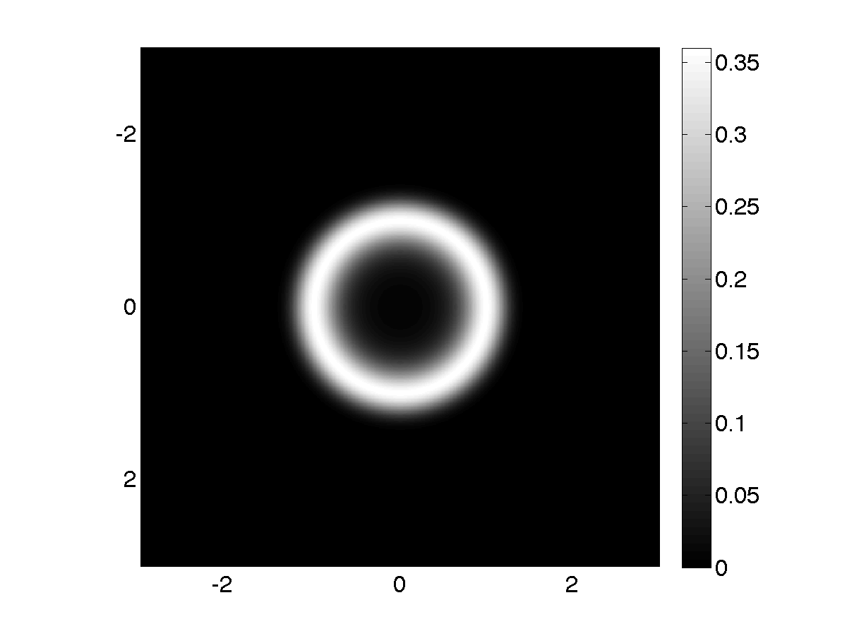
Figure 1: A plot of the annular distribution in 2D for $R=1$ and $\alpha=8$.

The distribution can clearly be shifted to a non-zero mean $\boldsymbol{\mu}$ and $\mathbf{x}^{T}\mathbf{x}$ can transformed to $\mathbf{x}^{T}\Sigma^{-1}\mathbf{x}$ for some SPD matrix $\Sigma$. I term the distribution in eq. 1 under this transformation the Elliptical Quartic Exponential distribution, by analogy with the Elliptical Gamma distribution discussed below; both have elliptical contours.

Below I discuss related work, analytical expressions for the normalization constant and the entropy, and the conditional and marginal distributions of the Elliptical Quartic Exponential distribution.

1.1 Related work

Fisher, (1922) discussed univariate probability densities having the form $p(x)\propto\exp(-Q_{k}(x))$, where $Q_{k}(x)=\sum_{q=1}^{k}\alpha_{q}x^{q}$, with $k$ even and $\alpha_{k}>0$. Matz, (1978) discusses the case with $k=4$ known as the quartic exponential distribution, and the special case of $p(x)\propto\exp(-\beta x^{2}-\gamma x^{4})$ with $\gamma>0$ and $\beta$ unrestricted in sign; this is termed the symmetric quartic exponential distribution. The quartic exponential distribution can be obtained via maximum entropy considerations given the first four moments, see e.g., Zellner and Highfield, (1988).

In the multivariate case, Urzúa, (1997) considers $p(\mathbf{x})\propto\exp(-Q(\mathbf{x}))$. If $Q(\mathbf{x})$ is a polynomial of degree $k$ in $D$ dimensions, it can be written as $Q(\mathbf{x})=\sum_{q=1}^{k}Q^{(q)}(\mathbf{x})$, where each $Q^{(q)}(\mathbf{x})$ is a homogeneous polynomial of degree $q$, i.e.

$$Q^{(q)}(\mathbf{x})=\sum\alpha^{(q)}_{j_{1}\ldots j_{D}}\prod_{i=1}^{D}x^{j_{i}}_{i},$$ (3)

with the summation taken over all non-negative integer $D$-tuples $(j_{1},\ldots,j_{D})$ such that $j_{1}+\ldots+j_{D}=q$. This is known as the multivariate quartic exponential distribution. The maximum possible number of parameters is determined as $(D+k)!/(D!k!)-1$. However, to my knowledge, the specific distribution in eq. 1 derived from the constraints on $r^{2}$ and $r^{4}$ only has not been discussed before in the literature.

Abramov, (2010) discusses numerical methods for obtaining the maximum entropy distribution given moment constraints.

Another route to defining an annular distribution is to first define an distribution on $r$ which is unimodal with its mode away from zero, and then to distribute that mass between $r$ and $r+dr$ over the spherical shell at this radius. Using this construction with the Gamma distribution gives rise to the Elliptical Gamma distribution (Koutras, 1986; see also Sra et al., 2015), defined as

$$p_{EG}(\mathbf{x};\Sigma,a,b) =\frac{\Gamma(D/2)}{\pi^{D/2}\Gamma(a)b^{a}|\Sigma|^{1/2}}\phi(\mathbf{x}^{T}\Sigma^{-1}\mathbf{x}),$$ (4)

where $\phi(t)=t^{a-D/2}e^{-t/b}$, $a,\,b>0$ and $\Sigma$ is a symmetric positive definite (SPD) matrix. Differentiation of $\phi(t)$ for $t=r^{2}=\mathbf{x}^{T}\Sigma^{-1}\mathbf{x}$ shows that it reaches a maximum at $r^{2}=b(a-D/2)$ for $a>D/2$, giving rise to an annular distribution quite similar to the Elliptical Quartic Exponential distribution.

1.2 Normalization constant

A remaining issue is to obtain an analytic expression for $Z_{D}(\lambda_{1},\lambda_{2})$. We have that

$$Z_{D}(\lambda_{1},\lambda_{2})=\int_{0}^{\infty}S_{D-1}r^{D-1}\;e^{(\lambda_{1}r^{2}-\lambda_{2}r^{4})}dr.$$ (5)

where $S_{n}$ denotes the surface area of the unit sphere in $n$-dimensions; for example the unit 1-sphere is the unit circle in $\mathbb{R}^{2}$, so $S_{1}=2\pi$. Now consider the change of variable $y=r^{2}$, with $dy=2rdr$. Hence

$$Z_{D}(\lambda_{1},\lambda_{2})=\frac{S_{D-1}}{2}\int_{0}^{\infty}y^{D/2-1}e^{(\lambda_{1}y-\lambda_{2}y^{2})}dy.$$ (6)

Gradshteyn and Ryzhik, (2007) equation 3.462.1 is

$$\int_{0}^{\infty}y^{\nu-1}e^{-\beta y^{2}-\gamma y}dy=(2\beta)^{-\nu/2}\Gamma(\nu)\exp(\frac{\gamma^{2}}{8\beta})D_{-\nu}(\frac{\gamma}{\sqrt{2\beta}}),$$ (7)

where $D_{\nu}$ is a Parabolic Cylinder Function (Gradshteyn and Ryzhik,, 2007, 9.24-9.25). Hence by identifying $\nu=D/2$, $\beta=\lambda_{2}$ and $\gamma=-\lambda_{1}$ we have that

$$Z_{D}(\lambda_{1},\lambda_{2})=\frac{S_{D-1}}{2}(2\lambda_{2})^{-D/4}\Gamma(D/2)\exp(\frac{\lambda_{1}^{2}}{8\lambda_{2}})D_{-D/2}(\frac{-\lambda_{1}}{\sqrt{2\lambda_{2}}}).$$ (8)

For $D=2$ or $\nu=1$ using the relationship $D_{-1}(z)=\sqrt{\frac{\pi}{2}}e^{z^{2}/4}[1-\Phi(\frac{z}{\sqrt{2}})]$ from Gradshteyn and Ryzhik, (2007, 9.254.1), where $\Phi(\cdot)$ denotes the error function (erf) $\Phi(x)=\frac{2}{\sqrt{\pi}}\int_{0}^{x}e^{-t^{2}}dt$, we have

$$Z_{2}(\lambda_{1},\lambda_{2})=\frac{\pi}{2}\sqrt{\frac{\pi}{\lambda_{2}}}\exp\left(\frac{\lambda_{1}^{2}}{4\lambda_{2}}\right)\left[1-\Phi(\frac{-\lambda_{1}}{2\sqrt{\lambda_{2}}})\right].$$ (9)

In eq. 8 a general expression for $Z_{D}(\lambda_{1},\lambda_{2})$ is given in terms of the Parabolic Cylinder Function $D_{\nu}$. It is of interest to see if this can be expressed in terms of more familiar functions for the case of $D=1$. As discussed in Matz, (1978, sec. 2), the cases of $\lambda_{1}\gtrless 0$ are considered separately. O’Toole, (1933, pp. 5-9) discusses the case for $\lambda_{1}>0$, and obtains a complicated expression involving the Bessel functions $J_{1/4}$ and $J_{-1/4}$. A series expansion (eq. 2) is also given which is recommended for computation. For $\lambda_{1}<0$, the integral 3.323.3 in Gradshteyn and Ryzhik, (2007) results in an expression involving the modified Bessel function $K_{1/4}$. Of course numerical quadrature is straightforward for the 1D case.

1.3 Entropy

We have that $-\log p(\mathbf{x})=\lambda_{2}(\mathbf{x}^{T}\mathbf{x})^{2}-\lambda_{1}(\mathbf{x}^{T}\mathbf{x})+\log Z_{D}(\lambda_{1},\lambda_{2})$, and hence that the entropy is given by

$$H(p)=\mathbb{E}_{p}[-\log p(\mathbf{x})]=\lambda_{2}\mathbb{E}_{p}[r^{4}]-\lambda_{1}\mathbb{E}_{p}[r^{2}]+\log Z_{D}(\lambda_{1},\lambda_{2}).$$ (10)

In general we have that

$$\mathbb{E}_{p}[r^{k}]=S_{D-1}\int_{0}^{\infty}r^{k+D-1}e^{(\lambda_{1}r^{2}-\lambda_{2}r^{4})}dr.$$ (11)

By using the change of variable $y=r^{2}$, this integral can be evaluated as per eq. 7 for $k=2$ and $k=4$, and hence the entropy can be computed.

1.4 Conditional distribution

Let $p(\mathbf{x})\propto e^{J(\mathbf{x})}$, where $J(\mathbf{x})=\lambda_{1}\mathbf{x}^{T}\mathbf{x}-\lambda_{2}(\mathbf{x}^{T}\mathbf{x})^{2}$. Now consider splitting $\mathbf{x}$ into two parts $\mathbf{x}=(\mathbf{x}_{1}^{T},\mathbf{x}_{2}^{T})^{T}$, so that $\mathbf{x}^{T}\mathbf{x}=\mathbf{x}_{1}^{T}\mathbf{x}_{1}+\mathbf{x}_{2}^{T}\mathbf{x}_{2}$. Hence

$$J(\mathbf{x}_{1},\mathbf{x}_{2})=\lambda_{1}(\mathbf{x}_{1}^{T}\mathbf{x}_{1}+\mathbf{x}_{2}^{T}\mathbf{x}_{2})-\lambda_{2}\left((\mathbf{x}_{1}^{T}\mathbf{x}_{1})^{2}+(\mathbf{x}_{2}^{T}\mathbf{x}_{2})^{4}+2(\mathbf{x}_{1}^{T}\mathbf{x}_{1})(\mathbf{x}_{2}^{T}\mathbf{x}_{2})\right).$$ (12)

Consider the conditional distribution $p(\mathbf{x}_{1}|\mathbf{x}_{2})\propto p(\mathbf{x}_{1},\mathbf{x}_{2})$ when keeping $\mathbf{x}_{2}$ fixed. Hence we obtain

$$p(\mathbf{x}_{1}|\mathbf{x}_{2})\propto\exp\left[(\lambda_{1}-2\lambda_{2}(\mathbf{x}_{2}^{T}\mathbf{x}_{2}))\mathbf{x}_{1}^{T}\mathbf{x}_{1}-\lambda_{2}(\mathbf{x}_{1}^{T}\mathbf{x}_{1})^{2}\right].$$ (13)

Let $\lambda^{\prime}_{1}=\lambda_{1}-2\lambda_{2}(\mathbf{x}_{2}^{T}\mathbf{x}_{2})$. Recall that $\lambda_{1}=2R^{2}\lambda_{2}$, hence $\lambda^{\prime}_{1}=\lambda_{1}(1-(\mathbf{x}_{2}^{T}\mathbf{x}_{2})/R^{2})$. If $(\mathbf{x}_{2}^{T}\mathbf{x}_{2})<R^{2}$ then $\lambda^{\prime}_{1}>0$ and the conditional distribution is an annular distribution. But if $(\mathbf{x}_{2}^{T}\mathbf{x}_{2})\geq R^{2}$ then $\lambda^{\prime}_{1}\leq 0$ the conditional distribution is a unimodal distribution centered at the origin.

For a geometric intuition, consider an annular distribution in $D=3$ dimensions, and condition on $x_{3}=c$ to obtain a 2D slice through the 3D dimension. If $c<R$ then this is an annular distribution, while for $c\geq R$ it is a unimodal distribution centered at the origin.

1.5 Marginal distribution

For simplicity we consider the 2D distribution with $\mathbf{x}^{T}\mathbf{x}=x_{1}^{2}+x_{2}^{2}$. Then

$$p(x_{1},x_{2})=\frac{1}{Z_{2}(\lambda_{1},\lambda_{2})}\exp\left(\lambda_{1}(x_{1}^{2}+x_{2}^{2})-\lambda_{2}(x_{1}^{4}+2x_{1}^{2}x_{2}^{2}+x_{2}^{4})\right).$$ (14)

Thus

$$p(x_{1}) =\int_{-\infty}^{\infty}p(x_{1},x_{2})dx_{2}$$ (15)

$$=\frac{1}{Z_{2}(\lambda_{1},\lambda_{2})}\exp(\lambda_{1}x_{1}^{2}-\lambda_{2}x_{1}^{4})\int_{-\infty}^{\infty}\exp((\lambda_{1}-2\lambda_{2}x_{1}^{2})x_{2}^{2}-\lambda_{2}x_{2}^{4})dx_{2}.$$ (16)

Let $\tilde{\lambda}_{1}=(\lambda_{1}-2\lambda_{2}x_{1}^{2})$. Observe that the integral above is equal $Z_{1}(\tilde{\lambda}_{1},\lambda_{2})$. Recalling that $\tilde{\lambda}_{1}=(\lambda_{1}-2\lambda_{2}x_{1}^{2})$ is a function of $x_{1}$, the expression for $Z_{1}(\tilde{\lambda}_{1},\lambda_{2})$ can be combined with the factors before the integral in eq.  16 to obtain the marginal distribution. A plot of the marginal distribution for the case shown in Figure 1 shows that it is bimodal, with peaks just inside $\pm R$.

This marginalization can be extended to multivariate $\mathbf{x}_{1},\,\mathbf{x}_{2}$ by replacing $x^{2}_{1}$ by $\mathbf{x}_{1}^{T}\mathbf{x}_{1}$, and similarly for $\mathbf{x}_{2}$. However, note that in the integration in eq. 16 there will be a factor of $S_{D_{2}-1}r_{2}^{D_{2}-1}$ coming in when changing coordinates to $r_{2}^{2}=\mathbf{x}^{T}_{2}\mathbf{x}_{2}$, corresponding to $Z_{D_{2}}(\tilde{\lambda}_{1},\lambda_{2})$.

References

• Abramov, (2010) Abramov, R.Β V. (2010). The Multidimensional Maximum Entropy Moment Problem: A Review on Numerical Methods. Commum. Math. Sci., 8(2):377–392.
• Cover and Thomas, (1991) Cover, T.Β M. and Thomas, J.Β A. (1991). Elements of Information Theory. Wiley.
• Fisher, (1922) Fisher, R.Β A. (1922). On the Mathematical Foundations of Theoretical Statistics. Phil. Trans. Roy. Soc. A, 222:309–368.