Label-Driven Denoising Framework for Multi-Label Few-Shot
Aspect Category Detection

Abstract

Multi-Label Few-Shot Aspect Category Detection (FS-ACD) is a new sub-task of aspect-based sentiment analysis, which aims to detect aspect categories accurately with limited training instances. Recently, dominant works use the prototypical network to accomplish this task, and employ the attention mechanism to extract keywords of aspect category from the sentences to produce the prototype for each aspect. However, they still suffer from serious noise problems: (1) due to lack of sufficient supervised data, the previous methods easily catch noisy words irrelevant to the current aspect category, which largely affects the quality of the generated prototype; (2) the semantically-close aspect categories usually generate similar prototypes, which are mutually noisy and confuse the classifier seriously. In this paper, we resort to the label information of each aspect to tackle the above problems, along with proposing a novel Label-Driven Denoising Framework (LDF). Extensive experimental results show that our framework achieves better performance than other state-of-the-art methods.

1 Introduction

Aspect Category Detection (ACD) is an important subtask of fine-grained sentiment analysis Pontiki et al. (2014), which aims to detect the aspect categories mentioned in a review sentence from a predefined set of aspect categories. For example, given the sentence “The service is good although rooms are pretty expensive.”, the ACD task is to detect two aspect categories from the sentence, respectively service and price. Obviously, the ACD belongs to a multi-label classification problem.

Support set
Aspect Category	Sentences
(A) food_food_meat_burger	(1) first time, burger was not fully cooked and my smash fries were cold.
	(2) food was over priced, but okay not great.
(B) food_mealtype_lunch	(1) my brother and i stopped in for lunch.
	(2) lunch has a great option of picking one or two food with rice.
(C) restaurant_location	(1) i prefer the other location to be honest.
	(2) there’s a new standard in town.
Query set
Aspect Category	Sentences
(B)	(1) went back today for lunch.
(A) and (C)	(2) food is whats to be expected at a neighborhood grill.

Table 1: An example of 3-way 2-shot meta-task. A sentence (instance) may belong to multiple aspects.

Recently, with the development of deep learning technique, a great number of neural models have been proposed for the ACD task Zhou et al. (2015); Schouten et al. (2018); Hu et al. (2019). The performance of all these models heavily rely on sufficient labeled data. However, the annotation of aspect categories in ACD is extremely expensive. The limited labeled data restrict the effectiveness of neural models. To alleviate the issue,  Hu et al. Hu et al. (2021) refer to few-shot learning (FSL) Ravi and Larochelle (2017); Finn et al. (2017); Snell et al. (2017); Gao et al. (2019) and formalize ACD as a few-shot ACD (FS-ACD) problem, learning aspect categories with limited supervised data.

FS-ACD follows the meta-learning paradigm Vinyals et al. (2016) and builds a collection of $N$-way $K$-shot meta-tasks. Table 1 shows a 3-way 2-shot meta-task, which consists of a support set and a query set. The support set samples three classes (i.e., aspect categories), and each class selects two sentences (instances). A meta-task aims to infer the classes of sentences in the query set with the help of the small labeled support set. By sampling different meta-tasks in the training stage, FS-ACD can learn great generalization ability in few-shot scenario and works well in the testing stage. To perform the FS-ACD task,  Hu et al. Hu et al. (2021) proposes an attention-based prototypical network Proto-AWATT. It first exploits an attention mechanism  Bahdanau et al. (2015) to extract keywords from the sentences corresponding to aspect category in the support set, and then aggregate them as evidence to generate a prototype for each aspect. Next, the query set utilizes the prototypes to generate corresponding query representations. Finally, the prediction is made by measuring the distance between each prototype representation and corresponding query representation in the embedding space.

Though achieving impressive progress, we find the noise is still a crucial problem for the FS-ACD task. The reason comes from two folds. On the one hand, the previous models easily catch noisy words irrelevant to the current aspect category due to the lack of sufficient supervised data, which largely affects the quality of the generated prototype. As shown in Figure 1, take the prototype of aspect category food_food_meat_burger as an example. We highlight its top-10 words based on attention weights of Proto-AWATT. Because of lacking sufficient supervised data, we observe the model tends to focus on these common but noisy words, such as “a”, “the”, “my”. These noisy words fail to produce a representative prototype for each aspect, resulting in the discounted performance. On the other hand, the semantically-close aspect categories usually produce similar prototypes, these close prototypes are mutually noisy and confuse the classifier greatly. According to the statistics, nearly 25% of aspect category pairs in the benchmark dataset have similar semantics, such as food_food_meat_burger and food_mealtype_lunch in Table 1. Apparently, the prototypes generated by these semantically-close aspect categories can interfere with each other and confuse the detection results of FS-ACD seriously.

To tackle the above issues, we propose a novel Label-Driven Denoising Framework (LDF) for the FS-ACD task. Specifically, for the first issue, the label text of aspect category contains rich semantics describing the concept and scope of aspect, such as the text “restaurant location” for the aspect restaurant_location, which intuitively help the attention capture label-relevant words better. Therefore, we propose a label-guided attention strategy to filter noisy words and guide LDF to yield better aspect prototypes. Given the second issue, we propose an effective label-weighted contrastive loss, which incorporates inter-class relationships of support set into a contrastive objective function, thereby enlarging the distance among similar prototypes.

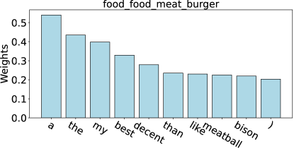
Figure 1: Visualization of the top-10 words for the prototype of aspect category food_food_meat_burger according to the attention weights of Proto-AWATT.

Our contributions are summarized as follows:

• To the best of our knowledge, we are the first to exploit the label information of each aspect to address noise problems in the FS-ACD task.

• We propose a novel Label-Driven Denoising Framework (LDF), which contains a label-guided attention strategy to filter noisy words and generate a representative prototype for each aspect, and a label-weighted contrastive loss to avoid generating similar prototypes for semantically-close aspect categories.

• The LDF framework has good compatibility and can be easily extended to existing models. In this work, we apply it to two latest FS-ACD models, Proto-HATT Gao et al. (2019) and Proto-AWATT Hu et al. (2021). Experimental results on three benchmark datasets prove the superiority of our framework.

2 Notations and Background

In this section, we first present the task formalization of FS-ACD and then give brief introductions to the background.

2.1 Task Formalization

The FS-ACD task follows the meta-learning paradigm Vinyals et al. (2016). Specifically, given labeled instances from a set of classes (i.e., aspect categories) $C_{train}$, the goal is to acquire knowledge from $C_{train}$ and use the knowledge to recognize novel classes, which have only a few labeled instances. These novel classes belong to a set of classes $C_{test}$ and disjoint from $C_{train}$.

To emulate the few-shot scenario, meta-learning algorithms learn from a group of $N$-way $K$-shot meta-tasks sampled from $C_{train}$. Within each meta-task, we randomly select $N$ classes ($N$-way) from $C_{train}$, each with $K$ instances ($K$-shot) to form a support set $\mathcal{S}=\{\mathbf{\emph{s}}_{k}^{n}\,|\,k=1,...,K\}_{n=1}^{N}$. Meanwhile, $M$ instances are sampled from the remaining data of the $N$ classes to construct a query set $\mathcal{Q}=\{(\mathbf{\emph{q}}_{i},\,\mathbf{\emph{y}}_{i})\,|\,\mathbf{\emph{y}}_{i}\in\mathbb{R}^{N}\}_{i=1}^{M}$, where $\mathbf{\emph{y}}_{i}$ is a binary label vector whose $n$-th bit is set to 1 if $\mathbf{\emph{q}}_{i}$ belongs to the $n$-th class (i.e., aspect category), 0 otherwise. A meta-task aims to infer the class(es) of query instance $\mathbf{\emph{q}}_{i}$ in $\mathcal{Q}$ according to a small labeled support set $\mathcal{S}$. By sampling different meta-tasks in the training stage, FS-ACD can learn great generalization ability. During the testing stage, we apply the same manner to test whether our model can adapt quickly to novel classes within $C_{test}$.

2.2 Background

In this work, we abstract a general attention architecture based on the Proto-AWATT Hu et al. (2021) and Proto-HATT Gao et al. (2019) models, which both achieve satisfying performance and thus are chosen as the foundations of our work.

Given a instance $\mathbf{\emph{s}}_{k}^{n}=\{w_{1},w_{2},...,w_{l}\}$ consisting $l$ words, we first map it into an word sequence $\mathbf{\emph{e}}_{k}^{n}=\{\mathbf{\emph{e}}_{1},\mathbf{\emph{e}}_{2},...,\mathbf{\emph{e}}_{l}\}$ by looking up an embedding table. And then, we apply a convolutional neural network (CNN) Zeng et al. (2014); Gao et al. (2019) to encode the word sequence into a contextual representation $H_{k}^{n}$. Next, an attention layer assigns a weight $\beta$ to each word in the instance. The final instance representation is given by:

$$\beta=\text{ATT}_{W}(\mathbf{\emph{H}}_{k}^{n}),$$ (1)

$$\mathbf{\emph{r}}_{k}^{n}=\beta\mathbf{\emph{H}}_{k}^{n},$$ (2)

where $H_{k}^{n}$ is the $k$-th instance representation of the class $n$ in the support set $\mathcal{S}$, $\text{ATT}_{W}(\cdot)$ denotes an attention mechanism. After that, we aggregate all instance representations for the class $n$ to produce the prototype:

$$\mathbf{\emph{r}}^{n}=\text{Aggregation}(\mathbf{\emph{r}}_{1}^{n},...,\mathbf{\emph{r}}_{K}^{n}),$$ (3)

where $\text{Aggregation}(\cdot)$ denotes the attention mechanism or average pooling operation. After processing all classes in the support set $\mathcal{S}$, we obtain $N$ prototypes $\{\mathbf{\emph{r}}^{1},\mathbf{\emph{r}}^{2},...,\mathbf{\emph{r}}^{n},...,\mathbf{\emph{r}}^{N}\}$.

Similarly, for a query instance $\mathbf{\emph{q}}_{i}$, we first encode $\mathbf{\emph{q}}_{i}$ to obtain its contextual representation, and then exploit an attention mechanism to produce $N$ prototype-specific query representations $\mathbf{\emph{r}}_{i}^{n}$ based on the $N$ prototypes. After that, we compute the Euclidean distance (ED) between each prototype and the corresponding prototype-specific query representation. Finally, we normalize the negative Euclidean distances to obtain the ranking of prototypes and use a threshold to select the positive predictions (i.e., aspect categories).

$$\hat{\mathbf{\emph{y}}_{i}}=\text{softmax}(-\text{ED}(\mathbf{\emph{r}}^{n},\mathbf{\emph{r}}_{i}^{n})),n\in[1,N]$$ (4)

The training objective is the mean square error (MSE) loss as follows:

$$\mathcal{L}_{mse}=\sum_{i=1}^{M}(\hat{\mathbf{\emph{y}}_{i}}-\mathbf{\emph{y}}_{i})^{2}$$ (5)

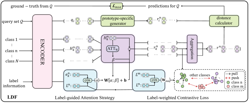
Figure 2: The overview of our proposed LDF framework.

3 Label-Driven Denoising Framework

Figure 2 shows the overall architecture of LDF, which contains two components: Label-guided Attention Strategy and Label-weighted Contrastive Loss. With the aid of label information, the former can focus on the class-relevant words better, thus producing a more accurate prototype for each class, the latter utilizes the inter-class relationships of support set to avoid generating similar prototypes.

3.1 Label-guided Attention Strategy

Due to lack of sufficient supervised data, the attention weights $\beta$ in Equation 1 usually focus on some noisy words irrelevant to the current class (i.e., aspect category), resulting in the prototype in Equation 3 becoming unrepresentative.

Intuitively, the label text of each class contains rich semantics, which can provide guidance for capturing class-relevant words. Thus, we leverage label information to tackle the above problem and propose a Label-guided Attention Strategy.

Specifically, we first locate the keywords of each class by calculating the semantic similarity between the label and each word in the instance:

$$\alpha=\text{cos}(\mathbf{\emph{L}}^{n},\mathbf{\emph{e}}_{k}^{n}),$$ (6)

where $\mathbf{\emph{L}}^{n}$ is the label embedding of class $n$ in the support set and calculated by averaging the multiple word embeddings of each class (e.g., food_food_meat_burger), $\mathbf{\emph{e}}_{k}^{n}$ is the word embedding of instance $\mathbf{\emph{s}}_{k}^{n}$, cos($\cdot$) is the cosine function.

Under the constraints of label information, the similarity weight $\alpha$ tends to focus on the limited words highly relevant to the label text and may neglect other informative words. Thus, we take it as the complementary information of the attention weights $\beta$ to generate a more comprehensive and accurate attention weight $\theta$. Formally,

$$\theta=W_{g}[\alpha;\beta]+b_{g}$$ (7)

where $W_{g}$ and $b_{g}$ are weight matrices and bias, $[\cdot\,;\cdot]$ denotes the concatenation operation.

Then, to regain the probabilistic attention distribution, the attention weight $\theta$ is re-normalized:

$$\widetilde{\theta}=\textrm{softmax}(\theta)$$ (8)

Finally, we replace $\beta$ in Equation 1 with the new attention vector $\widetilde{\theta}$ to obtain a representative prototype for each class in the support set.

3.2 Label-weighted Contrastive Loss

As mentioned before, the semantically-close aspect categories often generate similar prototypes in the support set, which are mutually noisy and confuse the classifier seriously.

Intuitively, a feasible and natural approach is to leverage supervised contrastive learning (CL) Khosla et al. (2020), which can push the prototype of different classes away as follows:

where $P(n,k)$ is the positive set of $r_{k}^{n}$ in Equation 2, which contains all the other samples (e.g., $r_{p}^{n}$) of the same class with $r_{k}^{n}$ in the support set. The rest of the ($N$-1)$\times K$ samples in the support set belong to the negative set, where $r_{k}^{m}$ is one negative sample from class $m$, $\tau$ is a temperature parameter.

However, the supervised CL does not well-resolve our problem since it treats different prototypes equally in the negative set, while our goal is to encourage the more similar prototypes to be farther apart. For example, “food_food_meat_burger” is semantically closer to “food_mealtype_lunch” than “room_bed”. Thus, “food_food_meat_burger” should be farther from “food_mealtype_lunch” than “room_bed” in the negative set.

To achieve this goal, we again leverage the label information and propose to incorporate inter-class relationships into the supervised CL to adaptively distinguish similar prototypes in the negative set:

where $w_{mn}$ denotes the cos similarity between different classes in the negative set and is computed as follows:

$$w_{mn}=\text{cos}(L^{m},L^{n}),$$ (11)

where $L^{m}$ and $L^{n}$ are the label embedding of the class $m$ and $n$. The final loss is formulated as:

$$\mathcal{L}=\mathcal{L}_{mse}+\lambda\mathcal{L}_{lcl}$$ (12)

where $\lambda$ is a hyper-parameter that measures the importance of $\mathcal{L}_{lcl}$ and can be adjusted.

4 Experimental Settings

4.1 Datasets and Implementation Details

To evaluate the effect of our framework, we carry out experiments on three datasets FewAsp(single), FewAsp(multi), and FewAsp from Hu et al. (2021), which share the same 100 aspects, with 64 aspects for training, 16 aspects for validation and 20 aspects for testing. It is notable that a sentence may belong to a single aspect or multiple aspects. FewAsp(single), FewAsp(multi), and FewAsp are composed of single-aspect, multi-aspect, and both types of sentences, respectively. General information for three datasets is presented in Table 2.

In each dataset, we construct four FS-ACD tasks, where $N$ = 5, 10 and $K$ = 5, 10. And the number of query instances per class is 5. All the models are implemented by the Tensorflow framework with an NVIDIA Tesla V100 GPU. The hyperparameters and training details are given in Appendix A.1.

4.2 Evaluation Metrics

Following Hu et al. (2021), we use Macro-F1 and AUC scores as our evaluation metrics, and the thresholds in the 5-way setting and 10-way setting are set to {0.3, 0.2}, respectively. Besides, the paired $t$-test is conducted to test the significance of different approaches. Finally, we report the average performance and standard deviation over 5 runs, where the seeds are set to [5, 10, 15, 20, 25]. Our code and datasets are available at https://github.com/1429904852/LDF.

4.3 Compared Methods

Following Hu et al. (2021), we chose some frequently-used baselines: Matching Network Vinyals et al. (2016), Prototypical Network Snell et al. (2017), Relation Network Sung et al. (2018), Graph Network Satorras and Estrach (2018), IMP Allen et al. (2019), Proto-HATT Gao et al. (2019) and Proto-AWATT Hu et al. (2021).

To verify the superiority of the LDF framework, we chose two dominant models with the best performance as the foundations of our work, i.e., Proto-HATT and Proto-AWATT. Finally, we integrate LDF into Proto-HATT and Proto-AWATT to obtain the model LDF-HATT and LDF-AWATT.

Dataset	#cls.	#inst./cls.	#inst.
FewAsp(single)	100	200	20000
FewAsp(multi)	100	400	40000
FewAsp	100	630	63000

Table 2: Statistics of three datasets. #cls. is the number of classes. #inst. is the total number of instances. #inst./cls. is the number of instances per class.

Models	5-way 5-shot		5-way 10-shot		10-way 5-shot		10-way 10-shot
	F1	AUC	F1	AUC	F1	AUC	F1	AUC
FewAsp
Proto-HATT	70.26	91.54	75.24	93.43	57.26	90.63	61.51	92.86
LDF-HATT	73.56${}^{\dagger}\pm$0.47	92.60${}^{\dagger}\pm$0.23	78.81${}^{\dagger}\pm$0.93	94.75${}^{\dagger}\pm$0.43	60.68${}^{\dagger}\pm$0.92	91.22$\pm$0.53	67.13${}^{\dagger}\pm$0.94	94.12${}^{\dagger}\pm$0.29
$\Delta$	+3.30	+1.06	+3.57	+1.32	+3.42	+0.59	+5.62	+1.26
Proto-AWATT	75.37	93.35	80.16	95.28	65.65	92.06	69.70	93.42
LDF-AWATT	78.27${}^{\dagger}\pm$0.89	94.65${}^{\dagger}\pm$0.41	81.87${}^{\dagger}\pm$0.48	95.71$\pm$0.26	67.13${}^{\dagger}\pm$0.41	92.74$\pm$0.12	71.97${}^{\dagger}\pm$0.49	94.29$\pm$0.25
$\Delta$	+2.90	+1.30	+1.71	+0.43	+1.48	+0.68	+2.27	+0.87
FewAsp(single)
Proto-HATT	83.33	96.45	86.71	97.62	73.42	95.71	77.65	97.00
LDF-HATT	84.41${}^{\dagger}\pm$0.46	97.06$\pm$0.16	88.15${}^{\dagger}\pm$1.00	98.12$\pm$0.31	76.27${}^{\dagger}\pm$1.08	96.38$\pm$0.37	80.54${}^{\dagger}\pm$0.97	97.45$\pm$0.14
$\Delta$	+1.08	+0.61	+1.44	+0.50	+2.85	+0.67	+2.89	+0.45
Proto-AWATT	86.71	97.56	88.54	97.96	80.28	97.01	82.97	97.55
LDF-AWATT	88.16${}^{\dagger}\pm$0.62	98.29$\pm$0.32	89.32$\pm$0.92	98.38$\pm$0.13	81.73${}^{\dagger}\pm$0.96	97.51$\pm$0.33	84.20${}^{\dagger}\pm$0.21	97.96$\pm$0.30
$\Delta$	+1.45	+0.73	+0.78	+0.42	+1.45	+0.50	+1.23	+0.41
FewAsp(multi)
Proto-HATT	69.15	91.10	73.91	93.03	55.34	90.44	60.21	92.38
LDF-HATT	72.13${}^{\dagger}\pm$0.79	92.19${}^{\dagger}\pm$0.33	76.52${}^{\dagger}\pm$0.74	93.68$\pm$0.36	59.10${}^{\dagger}\pm$1.04	91.00$\pm$0.51	65.31${}^{\dagger}\pm$0.57	92.99$\pm$0.24
$\Delta$	+2.98	+1.09	+2.61	+0.65	+3.76	+0.56	+5.10	+0.61
Proto-AWATT	71.72	91.45	77.19	93.89	58.89	89.80	66.76	92.34
LDF-AWATT	73.38${}^{\dagger}\pm$0.73	92.62${}^{\dagger}\pm$0.32	78.81${}^{\dagger}\pm$0.19	94.34$\pm$0.15	62.06${}^{\dagger}\pm$0.54	90.87${}^{\dagger}\pm$0.48	68.23${}^{\dagger}\pm$0.98	92.93$\pm$0.44
$\Delta$	+1.66	+1.17	+1.62	+0.44	+3.17	+1.07	+1.47	+0.59

Table 3: Test Macro-F1 and AUC score on the FewAsp, FewAsp(single), and FewAsp(multi) datasets (%). The results of Proto-HATT and Proto-AWATT are retrieved from Hu et al. (2021). We report the average performance and standard deviation over 5 runs, the thresholds in the 5-way setting and 10-way setting are set to {0.3, 0.2}. Best results are in bold. The marker ^† refers to significant test p-value $<$ 0.05 when comparing with Proto-HATT and Proto-AWATT. $\Delta$ denotes the difference between the performance of Proto-HATT and LDF-HATT, as well as Proto-AWATT and LDF-AWATT. Due to space constraints, we report other baseline results in Appendix A.2.

Models	5-way 5-shot		5-way 10-shot		10-way 5-shot		10-way 10-shot
	F1	AUC	F1	AUC	F1	AUC	F1	AUC
Proto-AWATT	75.37	93.35	80.16	95.28	65.65	92.06	69.70	93.42
Proto-AWATT+LAS	77.31$\pm$1.96	94.42$\pm$0.67	81.19$\pm$0.84	95.49$\pm$0.36	66.48$\pm$3.02	92.54$\pm$0.70	71.12$\pm$1.14	94.26$\pm$0.40
Proto-AWATT+LCL	77.06$\pm$0.71	94.20$\pm$0.26	80.78$\pm$0.39	95.44$\pm$0.22	66.20$\pm$1.26	92.38$\pm$0.45	70.83$\pm$0.66	94.07$\pm$0.33
Proto-AWATT+SCL	76.11$\pm$1.76	93.67$\pm$0.80	80.24$\pm$2.99	95.31$\pm$1.01	65.76$\pm$2.17	92.36$\pm$0.60	70.03$\pm$2.69	93.93$\pm$0.67
LDF-AWATT	78.27$\pm$0.89	94.65$\pm$0.41	81.87$\pm$0.48	95.71$\pm$0.26	67.13$\pm$0.41	92.74$\pm$0.12	71.97$\pm$0.49	94.29$\pm$0.25

Table 4: Ablation study over two main components on FewAsp dataset. The ablation results of FewAsp(single) and FewAsp(multi) datasets are included in Appendix A.3.

5 Results and Discussion

5.1 Main Results

The main experiment results are shown in Table 3. From this table, we can see that: (1) LDF-HATT and LDF-AWATT consistently outperform their base models on three datasets. It is worth mentioning that LDF-HATT at most obtains 5.62% and 1.32% improvements in Macro-F1 and AUC scores. In contrast, LDF-AWATT outperforms Proto-AWATT by 3.17% and 1.30% at most. These results reveal that our framework has good compatibility; (2) It is a fact that the Macro-F1 of LDF-AWATT is improved by about 2% in most settings, while that of LDF-HATT is improved by about 3% on average. This is consistent with our expectations since the original Proto-AWATT has a more powerful performance; (3) LDF-HATT and LDF-AWATT perform better on the FewAsp(multi) dataset than on the FewAsp(single) dataset. A possible reason is that each class in the FewAsp(multi) dataset contains more instances, which allows LDF-HATT and LDF-AWATT to generate a more accurate prototype in multi-label classification.

5.2 Ablation Study

Without loss of generality, we choose LDF-AWATT model for the ablation study to investigate the effects of different components in LDF.

Effect of Label-Driven Denoising Framework.

We study the two main components of LDF: Label-guided Attention Strategy (LAS) and Label-weighted Contrastive Loss (LCL). Based on the results in Table 4, we can make a couple of observations: (1) Compared to the base model Proto-AWATT, Proto-AWATT+LAS achieves competitive performance on three datasets, which validates the rationality of exploiting label information to generate a better prototype for each class; (2) After integrating LCL into Proto-AWATT+LAS, LDF-AWATT achieve the state-of-the-art performance, which demonstrates that LCL is beneficial to distinguish similar prototypes; (3) LAS is more effective than LCL. A possible reason is that the attention mechanism is the core factor in producing the prototype. Hence, it contributes more to our framework.

Analysis of Label in Contrastive Loss.

We compare Lable-weighted Contrastive Loss (LCL) with the Supervised Contrastive Loss (SCL) to see the contribution of label. It can be seen from Table 4 that: (1) Proto-AWATT+SCL performs slightly better than Proto-AWATT on FewAsp dataset, but their results are much lower than Proto-AWATT+LCL. These results further highlight the effectiveness of LCL; (2) After integrating inter-class relationships into Proto-AWATT+SCL, Proto-AWATT+LCL achieve better performance, which indicates that the inter-class relationships play a crucial role in distinguishing similar prototypes.

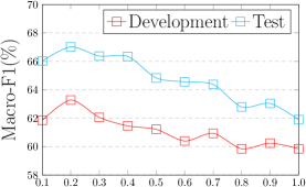
(a) FewAsp

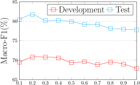
(b) FewAsp(single)

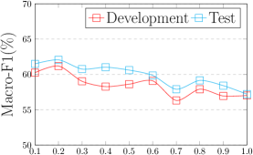
(c) FewAsp(multi)

Figure 3: Effect of $\lambda$ in the 10-way 5-shot setting on three dataset.

Models	GloVe + CNN		BERT
	F1	AUC	F1	AUC
Proto-HATT♣	57.26	90.63	57.33	89.70
LDF-HATT	60.68$\pm$0.92	91.22$\pm$0.53	63.72$\pm$0.27	91.99$\pm$0.12
Proto-AWATT♣	65.65	92.06	70.09	94.59
LDF-AWATT	67.13$\pm$0.41	92.74$\pm$0.12	72.76$\pm$0.29	95.31$\pm$0.19

Table 5: The effect of different encoders in the 10-way 5-shot scenario on FewAsp dataset. The results with symbol ^♣ are retrieved from Hu et al. (2021).

5.3 Discussion

Effect of Encoder.

We also conduct experiments (shown in Table 5) using the pre-trained BERT model Devlin et al. (2019). Concretely, we replace the Glove+CNN encoder with BERT and keep the other components the same as our original model. It’s clear that LDF-AWATT and LDF-HATT perform remarkably well than the base model Proto-AWATT and Proto-HATT on all encoders, which proves that our framework has good scalability.

Models	10-way 5-shot
	F1	AUC
Proto-AWATT	65.65	92.06
Proto-AWATT (LSW)	57.84$\pm$0.49	90.85$\pm$0.22

Table 6: The effect of label similarity weight $\alpha$ in the 10-way 5-shot scenario on FewAsp dataset.

Effect of Label Similarity Weight $\alpha$.

To illustrate the role of the similarity weight $\alpha$, we directly replace the attention weight $\beta$ in Equation 1 with the similarity weight $\alpha$ in Equation 6, and name this method as Proto-AWATT(LSW). From the results in Table 6, we can see that the performance of Proto-AWATT(LSW) is far inferior to Proto-AWATT, which implies that the similarity weight only plays a supporting role to the attention weight, and cannot be treated independently for the FS-ACD task.

Effect of hyper-parameter $\lambda$.

We tune the hyper-parameter $\lambda$ on the development set of each dataset, and then evaluate the performance of LDF-AWATT on the test set. Specifically, we conduct experiments for values set at 0.1 intervals in the range (0, 1). Figure 3 shows the performance of LDF-AWATT with different $\lambda$ on three dataset. Actually, as $\lambda$ increases, the performance of LDF-AWATT has an initial upward trend, and then flattens out or begins to fall. In the upward part, the Label-weighted Contrastive Loss (LCL) is useful guidance to help the LDF-AWATT distinguish similar prototypes more accurately, thus improving the performance. However, once the weight $\lambda$ exceeds 0.2, the LCL begins to dominate and performs poorly. The reason behind this may be that the bigger $\lambda$ has a negative effect on the MSE loss of the model. Therefore, we set $\lambda$ to be 0.2 on three datasets. In addition, we find that the best results of the development set and test set are basically consistent, which indicates that our framework has good robustness.

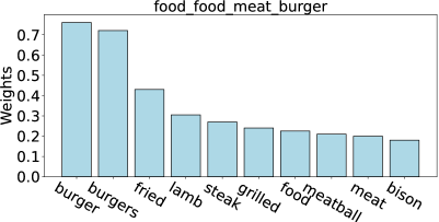
Figure 4: Visualize the top-10 words for the prototype of aspect category food_food_meat_burger based on the attention weights of Proto-AWATT+LAS.

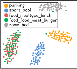
(a) Proto-AWATT

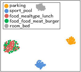
(b) Proto-AWATT+LAS

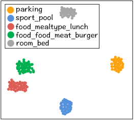
(c) LDF-AWATT

Figure 5: Visualization of prototype representations for Proto-AWATT, Proto-AWATT+LAS and LDF-AWATT.

5.4 Case Study

To better understand the advantage of our framework, we select some samples from FewAsp dataset for a case study. Specifically, we randomly sample 5 classes and then sample 50 times of 5-way 5-shot meta-tasks for the five classes. Finally for each class, we obtain 50 prototype vectors.

Proto-AWATT vs. Proto-AWATT+LAS.

As shown in Figure 5(a) and Figure 5(b), we can see that the prototype representation for each class learned by Proto-AWATT+LAS are obviously more concentrated than those by Proto-AWATT. Besides, in contrast to Proto-AWATT, Proto-AWATT+LAS can focus on class-relevant words better (shown in Figure 1 and Figure 4). These observations suggest that Proto-AWATT+LAS can indeed generate a more accurate prototype for each class.

Proto-AWATT+LAS vs. LDF-AWATT.

As depicted in Figure 5(b) and 5(c), after incorporating LCL into Proto-AWATT+LAS, the prototype representation of “food_mealtype_lunch” and “food_food_meat_burger” learned by LDF-AWATT are more separable than those by Proto-AWATT+LAS. This reveals that LCL can indeed distinguish similar prototypes.

5.5 Error Analysis

We present the error analysis in the Appendix A.4.

6 Related Work

Aspect Category Detection.

Previous works formulate ACD in a data-driven scenario, and can be generally divided into two kinds: one is unsupervised approach, which detects aspect categories by exploiting semantic association Su et al. (2006) or co-occurrence frequency Hai et al. (2011); Schouten et al. (2018); the other is supervised approach, which uses hand-crafted features Kiritchenko et al. (2014), learns useful representations automatically Zhou et al. (2015), adopts a multi-task learning strategy Hu et al. (2019), or utilizes a topic-attention model Movahedi et al. (2019) to address the ACD task. However, the above methods heavily rely on large-scale training data, which is time-consuming to annotate.

Multi-Label Few-Shot Learning.

In comparison with single-label FSL, multi-label FSL is more difficult and less explored, as it aims to identify multiple labels for an instance.  Rios and Kavuluru Rios and Kavuluru (2018) propose few-shot learning methods for multi-label text classification over a structured label space. Further research on multi-label FSL are developed on image synthesis  Alfassy et al. (2019), signal processing  Cheng et al. (2019), and intent detection  Hou et al. (2021). Recently,  Hu et al. Hu et al. (2021) formalize aspect category detection in a multi-label few-shot scenario to alleviate the dependency on large-scale labeled data. However,  Hu et al. Hu et al. (2021) ignore the label information of each class, which is crucial for generating a representative prototype in the FS-ACD task.

Contrastive Learning.

Contrastive Learning is a representation learning technique and has proven its effectiveness in the field of natural language processing Gunel et al. (2021); Kim et al. (2021); Ye et al. (2021). With the help of label information, Khosla et al. Khosla et al. (2020) propose supervised contrastive learning, which aims to improve the quality of learnt representations in a supervised setting. Different from their work, we do not treat label information equally and propose a label-weighted contrastive loss to distinguish similar prototypes.

7 Conclusion

In this paper, we propose a novel Label-Driven Denoising Framework (LDF) to alleviate the noise problems for the FS-ACD task. Specifically, we design two reasonable components: Label-guided Attention Strategy and Label-weighted Contrastive Loss, which aim to produce a better prototype for each class and distinguish similar prototypes. Results from numerous experiments indicate that our framework LDF achieves better performance than other state-of-the-art methods.

Limitations

We consider two major limitations in the FS-ACD task that need to be addressed in current research and related fields: (1) Existing studies for few-shot learning (FSL) require both the training and testing data have the same number of classes (denoted as $N$-way) and the same number of instances in each class (denoted as $K$-shot) in the support set. However, little investigation has been done towards inconsistent classes and inconsistent instances per class during training and testing. As far as we know, inconsistent FSL is more realistic and meaningful, which may be extremely helpful in low-resource scenarios; (2) The FS-ACD models usually give incorrect predictions when a sentence belongs to more than four aspect categories. A possible reason is that these sentences account for a small proportion of the dataset. Thus, it is also important to find effective methods to tackle the long-tail problem in multi-label classification. In general, the above limitations are of practical meaning and need us to do further research and exploration.

Appendix A Appendices

A.1 Implementation Details

Hyperparameters.

We initialize word embedding with 50-dimension Glove vectors. All other parameters are initialized by sampling from a normal distribution $\mathcal{N}(0,0.1)$. The hyper-parameter $\lambda$ is set to 0.2 on three datasets. The dimension of the hidden state is set to 50. The convolutional window size is set as 3. The optimizer is Adam with a learning rate 10^-3 and the temperature $\tau$ is set to 0.1. In each dataset, we construct four FS-ACD tasks, where N = 5, 10 and K = 5, 10. And the number of query instances per class is 5. For example, in a 5-way 10-shot meta-task, there are 5 $\times$ 10 = 50 instances in the support set and 5 $\times$ 5 = 25 instances in the query set.

Training Details.

During training, we train each model for a fixed 30 epochs, and then select the model with the best AUC score on the development set. Finally, we evaluate its performance on the test set. In every epoch, we randomly sample 800 meta-tasks for training. The number of meta-tasks during validation and testing are both set as 600. Besides, we employ an early stop strategy if the AUC score of the validation set is not improved in 3 epochs. For all baselines and our model, we report the average testing results from 5 runs, where the seeds are set to [5, 10, 15, 20, 25]. All the models are implemented by the Tensorflow framework with an NVIDIA Tesla V100 GPU.

Models	5-way 5-shot		5-way 10-shot		10-way 5-shot		10-way 10-shot
	F1	AUC	F1	AUC	F1	AUC	F1	AUC
FewAsp
Relation Network	59.52	85.56	62.78	86.98	45.62	84.94	44.70	83.77
Matching Network	67.14	90.76	70.09	92.39	51.27	88.44	54.61	89.90
Graph Network	61.49	89.48	69.89	92.35	47.91	87.35	56.06	90.19
Prototypical Network	66.96	88.88	73.27	91.77	52.06	87.35	59.03	90.13
IMP	68.96	89.95	74.13	92.30	54.14	88.50	59.84	90.81
Proto-HATT	70.26	91.54	75.24	93.43	57.26	90.63	61.51	92.86
LDF-HATT	73.56${}^{\dagger}\pm$0.47	92.60${}^{\dagger}\pm$0.23	78.81${}^{\dagger}\pm$0.93	94.75${}^{\dagger}\pm$0.43	60.68${}^{\dagger}\pm$0.92	91.22$\pm$0.53	67.13${}^{\dagger}\pm$0.94	94.12${}^{\dagger}\pm$0.29
Proto-AWATT	75.37	93.35	80.16	95.28	65.65	92.06	69.70	93.42
LDF-AWATT	78.27${}^{\dagger}\pm$0.89	94.65${}^{\dagger}\pm$0.41	81.87${}^{\dagger}\pm$0.48	95.71$\pm$0.26	67.13${}^{\dagger}\pm$0.41	92.74$\pm$0.12	71.97${}^{\dagger}\pm$0.49	94.29$\pm$0.25
FewAsp(single)
Relation Network	75.79	93.31	72.02	90.86	63.78	91.81	61.15	90.54
Matching Network	81.89	97.05	84.62	97.49	70.95	96.30	73.28	96.72
Graph Network	81.45	96.54	85.04	97.46	70.75	95.45	77.84	96.97
Prototypical Network	83.30	96.49	86.29	97.53	74.23	95.97	76.83	96.71
IMP	83.69	96.65	86.14	97.47	73.80	96.00	77.09	96.91
Proto-HATT	83.33	96.45	86.71	97.62	73.42	95.71	77.65	97.00
LDF-HATT	84.41${}^{\dagger}\pm$0.46	97.06$\pm$0.16	88.15${}^{\dagger}\pm$1.00	98.12$\pm$0.31	76.27${}^{\dagger}\pm$1.08	96.38$\pm$0.37	80.54${}^{\dagger}\pm$0.97	97.45$\pm$0.14
Proto-AWATT	86.71	97.56	88.54	97.96	80.28	97.01	82.97	97.55
LDF-AWATT	88.16${}^{\dagger}\pm$0.62	98.29$\pm$0.32	89.32$\pm$0.92	98.38$\pm$0.13	81.73${}^{\dagger}\pm$0.96	97.51$\pm$0.33	84.20${}^{\dagger}\pm$0.21	97.96$\pm$0.30
FewAsp(multi)
Relation Network	58.38	84.91	61.37	86.21	43.71	84.22	44.85	84.72
Matching Network	65.70	89.54	69.02	91.38	50.86	88.28	54.42	89.94
Graph Network	59.25	87.97	64.63	90.45	45.42	86.05	48.49	88.44
Prototypical Network	67.88	89.67	72.32	91.60	52.72	88.01	58.92	90.68
IMP	68.86	90.12	73.51	92.29	53.96	88.71	59.86	91.10
Proto-HATT	69.15	91.10	73.91	93.03	55.34	90.44	60.21	92.38
LDF-HATT	72.13${}^{\dagger}\pm$0.79	92.19${}^{\dagger}\pm$0.33	76.52${}^{\dagger}\pm$0.74	93.68$\pm$0.36	59.10${}^{\dagger}\pm$1.04	91.00$\pm$0.51	65.31${}^{\dagger}\pm$0.57	92.99$\pm$0.24
Proto-AWATT	71.72	91.45	77.19	93.89	58.89	89.80	66.76	92.34
LDF-AWATT	73.38${}^{\dagger}\pm$0.73	92.62${}^{\dagger}\pm$0.32	78.81${}^{\dagger}\pm$0.19	94.34$\pm$0.15	62.06${}^{\dagger}\pm$0.54	90.87${}^{\dagger}\pm$0.48	68.23${}^{\dagger}\pm$0.98	92.93$\pm$0.44

Table 7: Test Macro-F1 and AUC score on the FewAsp, FewAsp(single), and FewAsp(multi) datasets (%) . The baseline results are retrieved from Hu et al. (2021). We report the average performance and standard deviation over 5 runs, the thresholds in the 5-way setting and 10-way setting are set to {0.3, 0.2}. Best results are in bold. The marker ^† refers to significant test p-value $<$ 0.05 when comparing with Proto-HATT and Proto-AWATT.

A.2 Main Result

As shown in Table 7, we list all the frequently-used baselines and our enhanced version. It is clear that Proto-HATT and Proto-AWATT consistently outperform other baselines, thus we chose them as the foundation of our work. Besides, we observe that our framework achieves better performance compared to all the baselines.

A.3 Ablation Study

In Table 8 and 9, we present the ablation results of LDF-HATT and LDF-AWATT in details.

Models	5-way 5-shot		5-way 10-shot		10-way 5-shot		10-way 10-shot
	F1	AUC	F1	AUC	F1	AUC	F1	AUC
FewAsp
Proto-HATT	70.26	91.54	75.24	93.43	57.26	90.63	61.51	92.86
Proto-HATT+LAS	73.02$\pm$0.69	92.56$\pm$0.37	78.09$\pm$0.90	94.16$\pm$0.29	60.10$\pm$1.24	90.95$\pm$0.62	65.95$\pm$1.39	93.88$\pm$0.52
Proto-HATT+LCL	72.77$\pm$0.75	92.43$\pm$0.88	77.42$\pm$0.46	94.04$\pm$0.20	59.85$\pm$1.37	90.89$\pm$0.74	65.05$\pm$0.70	93.48$\pm$0.14
Proto-HATT+SCL	71.56$\pm$1.07	91.85$\pm$0.53	76.20$\pm$0.42	93.63$\pm$0.18	58.51$\pm$0.56	90.85$\pm$0.45	62.86$\pm$0.68	93.27$\pm$0.28
FewAsp(single)
Proto-HATT	83.33	96.45	86.71	97.62	73.42	95.71	77.65	97.00
Proto-HATT+LAS	83.96$\pm$0.23	96.92$\pm$0.27	87.80$\pm$1.02	98.12$\pm$0.30	75.82$\pm$0.49	96.15$\pm$0.14	79.90$\pm$1.04	97.24$\pm$0.24
Proto-HATT+LCL	83.89$\pm$0.81	96.88$\pm$0.27	87.54$\pm$1.19	97.86$\pm$0.36	75.48$\pm$0.61	96.12$\pm$0.14	79.66$\pm$1.05	97.16$\pm$0.55
Proto-HATT+SCL	83.35$\pm$0.70	96.80$\pm$0.23	86.96$\pm$0.79	97.67$\pm$0.44	74.60$\pm$0.47	96.00$\pm$0.16	78.55$\pm$1.06	97.16$\pm$0.18
FewAsp(multi)
Proto-HATT	69.15	91.10	73.91	93.03	55.34	90.44	60.21	92.38
Proto-HATT+LAS	71.44$\pm$0.54	91.74$\pm$0.25	76.17$\pm$1.14	93.50$\pm$0.45	58.50$\pm$0.65	90.72$\pm$0.48	64.76$\pm$0.83	92.62$\pm$0.47
Proto-HATT+LCL	71.15$\pm$0.38	91.59$\pm$0.10	75.86$\pm$0.49	93.47$\pm$0.58	57.90$\pm$0.96	90.50$\pm$0.45	64.65$\pm$0.72	92.57$\pm$0.47
Proto-HATT+SCL	70.37$\pm$0.39	91.41$\pm$0.15	74.82$\pm$0.88	93.32$\pm$0.50	56.72$\pm$0.91	90.49$\pm$0.40	62.77$\pm$0.96	92.40$\pm$0.37

Table 8: Ablation study over two main components of LDF-HATT. Besides, we also report the ablation result of Proto-HATT+LCL. We report the average performance and standard deviation over 5 runs.

Models	5-way 5-shot		5-way 10-shot		10-way 5-shot		10-way 10-shot
	F1	AUC	F1	AUC	F1	AUC	F1	AUC
FewAsp
Proto-AWATT	75.37	93.35	80.16	95.28	65.65	92.06	69.70	93.42
Proto-AWATT+LAS	77.31$\pm$0.96	94.42$\pm$0.36	81.19$\pm$0.84	95.49$\pm$0.36	66.48$\pm$1.32	92.54$\pm$0.64	71.12$\pm$1.14	94.26$\pm$0.40
Proto-AWATT+LCL	77.06$\pm$0.71	94.20$\pm$0.26	80.78$\pm$0.39	95.44$\pm$0.22	66.20$\pm$1.02	92.38$\pm$0.45	70.83$\pm$0.66	94.07$\pm$0.33
Proto-AWATT+SCL	76.11$\pm$0.92	93.67$\pm$0.55	80.24$\pm$0.60	95.31$\pm$0.25	65.76$\pm$0.97	92.36$\pm$0.33	70.03$\pm$1.15	93.93$\pm$0.21
FewAsp(single)
Proto-AWATT	86.71	97.56	88.54	97.96	80.28	97.01	82.97	97.55
Proto-AWATT+LAS	87.64$\pm$0.89	98.22$\pm$0.24	89.23$\pm$0.37	98.38$\pm$0.15	81.27$\pm$0.96	97.49$\pm$0.23	83.62$\pm$0.60	97.95$\pm$0.24
Proto-AWATT+LCL	87.44$\pm$0.88	98.09$\pm$0.25	89.08$\pm$0.73	98.31$\pm$0.11	81.11$\pm$0.95	97.49$\pm$0.13	83.29$\pm$0.94	97.93$\pm$0.22
Proto-AWATT+SCL	86.76$\pm$0.51	97.84$\pm$0.23	88.69$\pm$0.97	98.28$\pm$0.19	80.33$\pm$1.08	97.34$\pm$0.13	83.02$\pm$0.65	97.89$\pm$0.54
FewAsp(multi)
Proto-AWATT	71.72	91.45	77.19	93.89	58.89	89.80	66.76	92.34
Proto-AWATT+LAS	72.63$\pm$0.88	92.29$\pm$0.54	78.06$\pm$0.43	94.12$\pm$0.24	61.50$\pm$0.30	90.81$\pm$0.21	67.30$\pm$0.51	92.84$\pm$0.25
Proto-AWATT+LCL	72.61$\pm$0.82	92.08$\pm$0.36	77.78$\pm$0.92	93.92$\pm$0.53	60.42$\pm$0.47	89.93$\pm$0.37	67.12$\pm$0.78	92.52$\pm$0.67
Proto-AWATT+SCL	72.03$\pm$0.31	91.78$\pm$0.17	77.39$\pm$0.86	93.90$\pm$0.35	59.42$\pm$0.97	89.89$\pm$0.31	66.89$\pm$0.85	92.38$\pm$0.72

Table 9: Ablation study over two main components of LDF-AWATT. Besides, we also report the ablation result of Proto-AWATT+LCL. We report the average performance and standard deviation over 5 runs.

A.4 Error Analysis

To analyze the limitations of our framework, we randomly sample 100 error cases by LDF-AWATT from the FewAsp dataset, and roughly classify them into two categories. Table 10 shows the proportions and some representative examples for each category. The primary category is Complex, which includes examples that require deep comprehension to be understood. As shown in example (1), the word fragment “Chandler downtown Serrano” related to restaurant_location appears no more than five times in the dataset, the low frequency of those expressions makes it hard for our model to capture their patterns, so it is really challenging to give a right prediction. The second category is no obvious clues, which includes examples with insufficient information. As shown in example (2), the sentence is very short and unable to provide abundant information to predict the true label.

Through the error analysis, we can conclude that although current models have achieved appealing progress, there are still some complicated sentences beyond their capabilities. There ought to be more advanced natural language processing techniques to further address them.

Category	Proportion	Example	True Label	Predict Label
Complex	41%	(1) fast forward to december 2014, we have a company gathering in one of the many banquet rooms at the chandler downtown serrano.	restaurant_location	room_interior ✘
No obvious clues	22%	(2) overall, this is a great salon, and I will be back !	procedure_beauty_nails experience_wait	salon_interior_room ✘

Table 10: Error analysis of LDF-AWATT.

References

- Alfassy et al. (2019) Amit Alfassy, Leonid Karlinsky, Amit Aides, Joseph Shtok, Sivan Harary, Rogério Schmidt Feris, Raja Giryes, and Alexander M. Bronstein. 2019. Laso: Label-set operations networks for multi-label few-shot learning. In IEEE Conference on Computer Vision and Pattern Recognition, CVPR 2019, Long Beach, CA, USA, June 16-20, 2019, pages 6548–6557. Computer Vision Foundation / IEEE.
- Allen et al. (2019) Kelsey R. Allen, Evan Shelhamer, Hanul Shin, and Joshua B. Tenenbaum. 2019. Infinite mixture prototypes for few-shot learning. In Proceedings of the 36th International Conference on Machine Learning, ICML 2019, 9-15 June 2019, Long Beach, California, USA, volume 97 of Proceedings of Machine Learning Research, pages 232–241. PMLR.
- Bahdanau et al. (2015) Dzmitry Bahdanau, Kyunghyun Cho, and Yoshua Bengio. 2015. Neural machine translation by jointly learning to align and translate. In 3rd International Conference on Learning Representations, ICLR 2015, San Diego, CA, USA, May 7-9, 2015, Conference Track Proceedings.
- Cheng et al. (2019) Kai-Hsiang Cheng, Szu-Yu Chou, and Yi-Hsuan Yang. 2019. Multi-label few-shot learning for sound event recognition. In 21st IEEE International Workshop on Multimedia Signal Processing, MMSP 2019, Kuala Lumpur, Malaysia, September 27-29, 2019, pages 1–5. IEEE.
- Devlin et al. (2019) Jacob Devlin, Ming-Wei Chang, Kenton Lee, and Kristina Toutanova. 2019. BERT: pre-training of deep bidirectional transformers for language understanding. In NAACL 2019, pages 4171–4186. Association for Computational Linguistics.
- Finn et al. (2017) Chelsea Finn, Pieter Abbeel, and Sergey Levine. 2017. Model-agnostic meta-learning for fast adaptation of deep networks. In Proceedings of the 34th International Conference on Machine Learning, ICML 2017, Sydney, NSW, Australia, 6-11 August 2017, volume 70 of Proceedings of Machine Learning Research, pages 1126–1135. PMLR.
- Gao et al. (2019) Tianyu Gao, Xu Han, Zhiyuan Liu, and Maosong Sun. 2019. Hybrid attention-based prototypical networks for noisy few-shot relation classification. In The Thirty-Third AAAI Conference on Artificial Intelligence, AAAI 2019, The Thirty-First Innovative Applications of Artificial Intelligence Conference, IAAI 2019, The Ninth AAAI Symposium on Educational Advances in Artificial Intelligence, EAAI 2019, Honolulu, Hawaii, USA, January 27 - February 1, 2019, pages 6407–6414. AAAI Press.
- Gunel et al. (2021) Beliz Gunel, Jingfei Du, Alexis Conneau, and Veselin Stoyanov. 2021. Supervised contrastive learning for pre-trained language model fine-tuning. In 9th International Conference on Learning Representations, ICLR 2021, Virtual Event, Austria, May 3-7, 2021. OpenReview.net.
- Hai et al. (2011) Zhen Hai, Kuiyu Chang, and Jung-Jae Kim. 2011. Implicit feature identification via co-occurrence association rule mining. In Computational Linguistics and Intelligent Text Processing - 12th International Conference, CICLing 2011, Tokyo, Japan, February 20-26, 2011. Proceedings, Part I, volume 6608 of Lecture Notes in Computer Science, pages 393–404.
- Hou et al. (2021) Yutai Hou, Yongkui Lai, Yushan Wu, Wanxiang Che, and Ting Liu. 2021. Few-shot learning for multi-label intent detection. In Thirty-Fifth AAAI Conference on Artificial Intelligence, AAAI 2021, Thirty-Third Conference on Innovative Applications of Artificial Intelligence, IAAI 2021, The Eleventh Symposium on Educational Advances in Artificial Intelligence, EAAI 2021, Virtual Event, February 2-9, 2021, pages 13036–13044. AAAI Press.
- Hu et al. (2021) Mengting Hu, Shiwan Zhao, Honglei Guo, Chao Xue, Hang Gao, Tiegang Gao, Renhong Cheng, and Zhong Su. 2021. Multi-label few-shot learning for aspect category detection. In ACL/IJCNLP 2021, pages 6330–6340. Association for Computational Linguistics.
- Hu et al. (2019) Mengting Hu, Shiwan Zhao, Li Zhang, Keke Cai, Zhong Su, Renhong Cheng, and Xiaowei Shen. 2019. CAN: constrained attention networks for multi-aspect sentiment analysis. In EMNLP-IJCNLP 2019, Hong Kong, China, November 3-7, 2019, pages 4600–4609.
- Khosla et al. (2020) Prannay Khosla, Piotr Teterwak, Chen Wang, Aaron Sarna, Yonglong Tian, Phillip Isola, Aaron Maschinot, Ce Liu, and Dilip Krishnan. 2020. Supervised contrastive learning. In Advances in Neural Information Processing Systems 33: Annual Conference on Neural Information Processing Systems 2020, NeurIPS 2020, December 6-12, 2020, virtual.
- Kim et al. (2021) Taeuk Kim, Kang Min Yoo, and Sang-goo Lee. 2021. Self-guided contrastive learning for BERT sentence representations. In Proceedings of the 59th Annual Meeting of the Association for Computational Linguistics and the 11th International Joint Conference on Natural Language Processing, ACL/IJCNLP 2021, (Volume 1: Long Papers), Virtual Event, August 1-6, 2021, pages 2528–2540.
- Kiritchenko et al. (2014) Svetlana Kiritchenko, Xiaodan Zhu, Colin Cherry, and Saif Mohammad. 2014. Nrc-canada-2014: Detecting aspects and sentiment in customer reviews. In Proceedings of the 8th International Workshop on Semantic Evaluation, SemEval@COLING 2014, Dublin, Ireland, August 23-24, 2014, pages 437–442. The Association for Computer Linguistics.
- Movahedi et al. (2019) Sajad Movahedi, Erfan Ghadery, Heshaam Faili, and Azadeh Shakery. 2019. Aspect category detection via topic-attention network. CoRR, abs/1901.01183.
- Pontiki et al. (2014) Maria Pontiki, Dimitris Galanis, John Pavlopoulos, Harris Papageorgiou, Ion Androutsopoulos, and Suresh Manandhar. 2014. Semeval-2014 task 4: Aspect based sentiment analysis. In Proceedings of the 8th International Workshop on Semantic Evaluation, pages 27–35.
- Ravi and Larochelle (2017) Sachin Ravi and Hugo Larochelle. 2017. Optimization as a model for few-shot learning. In 5th International Conference on Learning Representations, ICLR 2017, Toulon, France, April 24-26, 2017, Conference Track Proceedings. OpenReview.net.
- Rios and Kavuluru (2018) Anthony Rios and Ramakanth Kavuluru. 2018. Few-shot and zero-shot multi-label learning for structured label spaces. In Proceedings of the 2018 Conference on Empirical Methods in Natural Language Processing, Brussels, Belgium, October 31 - November 4, 2018, pages 3132–3142. Association for Computational Linguistics.
- Satorras and Estrach (2018) Victor Garcia Satorras and Joan Bruna Estrach. 2018. Few-shot learning with graph neural networks. In 6th International Conference on Learning Representations, ICLR 2018, Vancouver, BC, Canada, April 30 - May 3, 2018, Conference Track Proceedings.
- Schouten et al. (2018) Kim Schouten, Onne van der Weijde, Flavius Frasincar, and Rommert Dekker. 2018. Supervised and unsupervised aspect category detection for sentiment analysis with co-occurrence data. IEEE Trans. Cybern., 48(4):1263–1275.
- Snell et al. (2017) Jake Snell, Kevin Swersky, and Richard S. Zemel. 2017. Prototypical networks for few-shot learning. In Advances in Neural Information Processing Systems 30: Annual Conference on Neural Information Processing Systems 2017, December 4-9, 2017, Long Beach, CA, USA, pages 4077–4087.
- Su et al. (2006) Qi Su, Kun Xiang, Houfeng Wang, Bin Sun, and Shiwen Yu. 2006. Using pointwise mutual information to identify implicit features in customer reviews. In Computer Processing of Oriental Languages. Beyond the Orient: The Research Challenges Ahead, 21st International Conference, ICCPOL 2006, Singapore, December 17-19, 2006, Proceedings, volume 4285 of Lecture Notes in Computer Science, pages 22–30.
- Sung et al. (2018) Flood Sung, Yongxin Yang, Li Zhang, Tao Xiang, Philip H. S. Torr, and Timothy M. Hospedales. 2018. Learning to compare: Relation network for few-shot learning. In 2018 IEEE Conference on Computer Vision and Pattern Recognition, CVPR 2018, Salt Lake City, UT, USA, June 18-22, 2018, pages 1199–1208. Computer Vision Foundation / IEEE Computer Society.
- Van der Maaten and Hinton (2008) Laurens Van der Maaten and Geoffrey Hinton. 2008. Visualizing data using t-sne. Journal of machine learning research, 9(11).
- Vinyals et al. (2016) Oriol Vinyals, Charles Blundell, Tim Lillicrap, Koray Kavukcuoglu, and Daan Wierstra. 2016. Matching networks for one shot learning. In Advances in Neural Information Processing Systems 29: Annual Conference on Neural Information Processing Systems 2016, December 5-10, 2016, Barcelona, Spain, pages 3630–3638.
- Ye et al. (2021) Seonghyeon Ye, Jiseon Kim, and Alice Oh. 2021. Efficient contrastive learning via novel data augmentation and curriculum learning. In Proceedings of the 2021 Conference on Empirical Methods in Natural Language Processing, EMNLP 2021, Virtual Event / Punta Cana, Dominican Republic, 7-11 November, 2021, pages 1832–1838. Association for Computational Linguistics.
- Zeng et al. (2014) Daojian Zeng, Kang Liu, Siwei Lai, Guangyou Zhou, and Jun Zhao. 2014. Relation classification via convolutional deep neural network. In COLING 2014, 25th International Conference on Computational Linguistics, Proceedings of the Conference: Technical Papers, August 23-29, 2014, Dublin, Ireland, pages 2335–2344. ACL.
- Zhou et al. (2015) Xinjie Zhou, Xiaojun Wan, and Jianguo Xiao. 2015. Representation learning for aspect category detection in online reviews. In Proceedings of the Twenty-Ninth AAAI Conference on Artificial Intelligence, January 25-30, 2015, Austin, Texas, USA, pages 417–424. AAAI Press.