Granite: A Graph Neural Network Model for
Basic Block Throughput Estimation

Abstract

Analytical hardware performance models yield swift estimation of desired hardware performance metrics. However, developing these analytical models for modern processors with sophisticated microarchitectures is an extremely laborious task and requires a firm understanding of target microarchitecture’s internal structure. In this paper, we introduce Granite, a new machine learning model that estimates the throughput of basic blocks across different microarchitectures. Granite uses a graph representation of basic blocks that captures both structural and data dependencies between instructions. This representation is processed using a graph neural network that takes advantage of the relational information captured in the graph and learns a rich neural representation of the basic block that allows more precise throughput estimation. Our results establish a new state-of-the-art for basic block performance estimation with an average test error of 6.9$\%$ across a wide range of basic blocks and microarchitectures for the x86-64 target. Compared to recent work, this reduced the error by 1.7$\%$ wile improving training and inference throughput by approximately 3.0$\times$. In addition, we propose the use of multi-task learning with independent multi-layer feed forward decoder networks. Our results show that this technique further improves precision of all learned models while significantly reducing per-microarchitecture training costs. We perform an extensive set of ablation studies and comparisons with prior work, concluding a set of methods to achieve high accuracy for basic block performance estimation.

1 Introduction

A basic block is a sequence of instructions with neither incoming nor outgoing branches. Basic blocks are natural input objects to many code optimization algorithms because the instructions of a basic block can be modified, as long as the invariants at the beginning and at the end of the basic block are preserved. See Table 1 for an example basic block. Accurate and fast performance estimation of basic blocks is often crucial at the various stages of compilation and software optimization [1, 2, 3, 4, 5, 6, 7] because real hardware measurements are expensive to collect and tedious to obtain. For example, various performance estimation methods are used for inlining [8], register allocation [1], fusing [9], hardware-software co-design [10, 11, 12, 13], and critical path analysis [14]. To provide a fast performance estimation, hand-tuned analytical models [15, 16, 17, 18], tailored for one or few sets of microarchitectures, have been developed. However, these analytical models are often lack generality across different processors and require domain expertise and thorough knowledge of internal organization of microarchitectural components, which are generally obscured by hardware companies. Even with sufficient domain knowledge, developing a complete and thorough analytical model for modern processors is an error-prone and work-intensive task. In addition, due to the increasing complexity of modern microarchitectures, these analytical models may overlook some corner cases in performance estimation and underperform in generalizing the estimation to these cases. As such, using the analytical models can mislead the optimization algorithm and yield sub-optimal solutions.

Learned models for throughput estimation. To address the aforementioned challenges, a handful of work delegated the task of performance estimation to machine learning [11, 12, 8]. For basic block throughput estimation specifically, Ithemal [19] uses a machine learning model based on a sequential Long-Short Term Memory (LSTM) to learn a representation of basic blocks followed by a linear transformation to predict the throughput values. While Ithemal [19] delivered a notable accuracy improvement across multiple x86-64 microarchitectures compared to analytical models of the time, it represents a basic block as a sequence of instructions without any additional information about its structure. We argue that adding information such as data dependency could contribute to the inductive bias of a model and enables the model to reason about code with higher accuracy.

Graph-based representation learning of basic blocks. Data and control flow in basic blocks can be naturally expressed using a graph [20]. This paper sets out to use graph neural networks on this representation of code to learn an expressive representation of basic blocks. The proposed representation learning method, dubbed Granite, does not commit to any feature engineering of the input basic blocks. Compared to prior work, we believe that leveraging a graph representation is a more natural and intuitive approach to represent basic blocks, better capturing the dependencies and interactions between instructions.

Granite outperforms Ithemal [19] in terms of accuracy and establishes a new state-of-the-arts results on x86-64 basic block throughput estimation. We evaluate Granite for the task of throughput estimation, achieving a new state of the art accuracy, with a nearly $1.7\%$ lower MAPE across multiple x86-64 microarchitectures, compared to the most recent prior work [19]. We argue that using a graph representation of basic blocks is a key contributing factor in achieving higher prediction accuracy, which is a direct consequence of better generalization to unseen basic blocks.

Multi-task throughput estimation model. While there are differences in performance of different microarchitectures, there are often also many similarities because of how their design evolved, but also due to instruction set semantics that are microarchitecture-independent. Multi-task learning [21] is a technique that uses a collection of related tasks to train the same model. By exploiting the relatedness of the tasks, the model learns a better internal representation of the problem domain and it often leads to improved performance on the individual tasks. To our best knowledge, existing work [19] did not take full advantage of these similarities and focused on developing or training a separate model for each target microarchitecture. We argue that the similarities between microarchitectures can be exploited to achieve faster training and learning richer representations of code. To this end, we propose a multi-headed task-dedicated representation learning where the graph network is shared by all microarchitectures and each head is trained for a different microarchitecture.

We evaluated a multi-task model against models that were trained only for a single microarchitecture. Our results demonstrate that it is feasible to learn a shared representation of basic blocks that support performance predictions for all target microarchitectures. The computational costs of training a model supporting multiple microarchitectures are only marginally higher than the cost of training a single single-task model. In addition, we found that employing multi-task learning further reduces the prediction errors on all microarchitectures compared to training exclusively on data from a single microarchitecture.

2 Motivation and Background

Table 1: An example basic block in x86-64 assembly from the BHive dataset [22].

0:	CMP	R15D, 1
1:	SBB	EAX, EAX
2:	AND	EAX, 0x8
3:	TEST	ECX, ECX
4:	MOV	DWORD PTR[RBP - 3], EAX
5:	MOV	EAX, 1
6:	CMOVG	EAX, ECX
7:	CMP	EDX, EAX

2.1 Manual Tuning of Simulator Parameters

Recent work [18] proposes an analytical model to predict the throughput of basic blocks for Intel microarchitectures with sufficient accuracy (< 1$\%$). To develop this analytical model, the authors performed a detailed study of the underlying Intel microarchitectures and manually tuned the microarchitecture-specific parameters of their simulator to match the ground-truth values. The suggested analytical model establishes stronger baselines for learned throughput estimation across a limited set of microarchitectures and provides interpretable insights about the underlying bottlenecks of the target microarchitecture. However, the hand-tuned analytical models generally suffer from: (1) a lack of generality across wide-range of unseen microarchitectures, (2) a tedious task of maintaining such an analytical model after each generation of microarchitectures, and finally (3) the demand of expert knowledge about the details of the underlying microarchitecture. On the other hand, learned models (such as our work and Ithemal [19]), marginally trade off prediction accuracy and interpretability of the results for generality across wide range of microarchitectures and eliminating the need for expert knowledge in the development process. In summary, analytical and learned models have different objectives and could be beneficial in downstream tasks with different objectives.

2.2 Learned Model for Throughput Estimation

Ithemal [19], the most recent learned model for basic block throughput estimation, formulates the throughput estimation problem as a regression problem with the objective to minimize the mean absolute percentage error between ground-truth data (obtained from hardware measurements) and the output of the learned model. It employs a two-level LSTM [23] network that generates an embedding vector for each input basic block. The objective of the first level LSTM network is to generate an embedding vector for each instruction of the input basic block. The second level uses the instruction embedding vectors to compute an embedding vector for the whole basic block.

In the input, Ithemal receives a sequence of instructions for each basic block (e.g. “SBB EAX, EAX”, as illustrated in Table 1). When presenting instructions to the model, Ithemal tokenizes each assembly instruction into (1) instruction mnemonic, (2) input operands, and (3) output operands. For example, “SBB EAX, EBX” is tokenized as “SBB | <S> | EAX | EBX | <D> | EAX | <E>” tokens, where “<S>”, “<D>”, and “<E>” are special tokens that separate the three groups of tokens. Each token is mapped to a learned embedding vector (each embedding vector is a real-valued vector of a fixed size), and these vectors are fed to the first-level LSTM network. Finally, the generated instruction embeddings pass through the second LSTM layer to obtain an embedding vector per basic block. The generated basic block embedding is then passed to a decoder network to obtain an estimation of the basic block throughput. In the Ithemal model, the decoder is a dot product of the basic block embedding vector with a vector of learned weights.

While Ithemal demonstrates a promising path forward for performance estimation of basic blocks, its input data format presents the instructions to the model linearly, as they are laid out in memory, and it relies on the model and the training process to discover dependencies between the instructions on it own. Since these dependencies are well defined and easy to extract using existing tools, we suggest including them in the basic block representation explicitly, to guide the computation of the model. This work wields graphs as a natural and intuitive way to represent basic blocks and the underlying dependencies, expecting that a graph neural network model will be able to benefit from the additional information and produce more precise throughput estimates.

2.3 Graph Neural Network

The family of graph neural networks (GNNs) [24, 25, 26, 27, 28] has shown to be effective in a diverse range of applications and domains [29, 30, 31, 32]. Generally, GNNs yield promising results in applications with highly structured inputs where the relationships between elements of the input can be easily expressed using a graph. The main objective of a GNN is to learn to map the information structured as a graph into an embedding space (a vector representation). In a nutshell, the learning process of a GNN model consists of propagating information between graph nodes and edges via multiple message passing iterations, followed by an aggregation step. At each message passing iteration, the node and edge embeddings are updated according to received messages from their neighbors in the graph. The final learned embeddings are then employed in downstream tasks such as regression, classification, and ranking.

3 Granite Model Architecture

The Granite model is composed of the following building blocks:

• Graph encoding of basic blocks $\rightarrow$ The first step in Granite is to transform basic blocks into a graph representation and convert the instructions and basic block dependencies into node and edge labels according to their types. The constructed graph representation for basic blocks is used as input to the graph neural network.

• Graph neural network $\rightarrow$ Next, Granite uses a GNN model with the objective to learn an expressive embedding for each basic block. As part of the training process, the GNN model iteratively exchanges relevant information between basic block elements with the objective of computing the embedding vectors.

• Decoder network $\rightarrow$ Each instruction embedding vector passes through an additional decoder network with non-linearity that computes the contribution of the instruction to the basic block throughput. Granite predicts the final throughput values for each basic block by adding all individual instructions’ contributions to the overall throughput.

• Multi-task decoder network $\rightarrow$ The multi-task version of Granite uses a multi-task decoder that predicts the throughput values across multiple microarchitectures simultaneously. Other parts of the model are shared across all target microarchitectures. Intuitively, the task of the shared parts is to learn an internal representation of basic block structure, while the decoder networks are responsible for throughput estimation.

3.1 Graph Encoding of Basic Blocks

We model each basic block as a dependency graph inspired by [20], but using a more compact format. The Granite graph is designed to capture the semantic relationships between instructions as well as the type and category of instructions and registers. The nodes of the graph consist of a set of instruction and value nodes (e.g. values in registers, immediate values, etc.), whereas the edges indicate data and structural dependencies between the instructions and values represented by the nodes. Figure 1 shows an example basic block in the Granite encoding.

Each node of the graph corresponds to an element of the assembly language, similar to one token in the Ithemal model [19]. Broadly, we can categorize node types into two groups: instruction nodes that represent instructions, and value nodes that model the input and output values passed between instructions. Table 2 summarizes the node types in Granite graph representation and assembly language tokens that can be associated with them. We represent each assembly instruction by a unique instruction mnemonic node. Infrequently, an assembly instruction may have prefixes that modify their behavior, such as “LOCK” or “REP”. We represent each prefix by a separate graph node that is connected to the instruction mnemonic node by an edge.

Each instruction node is connected to zero or more value nodes representing the instruction operands. The operands are values stored in registers or memory, immediate values, and results of address computation. Each value node has zero or one incoming edge from the instruction mnemonic node of the instruction that produces it (no incoming edge means that the value is not produced by an instruction of the block), and zero or more outgoing edges to instructions that consume the value. These edges represent the data dependencies between instructions. The token associated with a value node is the name of a register if the value is stored in a register, or a special token if the value is stored in memory, it is an immediate value, or it is the result of an address computation.

Note that the nodes represent a value in a storage location, not the storage location itself and the graph may contain multiple value nodes with a given register name, if multiple instructions in the block write to this register. For example, in Figure 1, register “RAX” is a destination operand for “MOV” instruction and is used as a source operand to calculate the memory address for “ADD” instruction. In the same example, you can see two different “Memory” nodes; one is used as an input operand, the other as an output operand. Since the value written by the “ADD” instruction maybe different from the value it reads, they are represented as two distinct nodes.

Table 3 summarizes the list of all edge types in the Granite graph representation. In a nutshell, the existence of an edge between two graph nodes captures the semantic relationships of the connected nodes as well as their sequential ordering. As such, all the edges in the graph are directed. The last column in Table 3 depicts the color code that we used to show the dependency between graph nodes in the example of a basic block in Figure 1.

3.2 Graph Neural Network

The objective of a graph neural network model is to learn representative feature vectors for graph nodes and edges that express their underlying characteristics in a latent space. The graph neural network propagates information between graph elements through message passing iterations. Before training starts, the graph elements (e.g. nodes and edges) are initialized to unique vector values that are representative of a particular property of each graph element. Granite uses the “full GN block” architecture as described in Section 4.2 of [28]. In each message passing iteration, all feature vectors are updated using Algorithm 1 from [28], employing multi-layer feed forward ReLU networks with residual connections [33] and layer normalization [34] at input as update functions. The initial values of the feature vectors of elements of the graph depend on the type of the element and the associated elements of the assembly language:

Table 2: The node types in Granite graph representation.

Node Type	Token
Instruction Nodes
Mnemonic	The mnemonic of the instruction (e.g. ADD).
Prefix	The prefix of an instruction (e.g. LOCK)
Value Nodes
Register	Register name (e.g. RBX).
FP immediate value	Special token shared by all floating-point immediate values.
Immediate value	Special token shared by all immediate value nodes.
Address computation	Special token shared by all address computation nodes.
Memory value	Special token shared by all values stored in memory.

Table 3: The edge types in Granite graph representation.

Edge Type	Description	Color Code
Structural Dependency	From an instruction mnemonic node to the instruction mnemonic node of the following instruction.
Input Operand	From a value node to an instruction mnemonic node.
Output Operand	From an instruction mnemonic node to a register or a memory value node.
Address Base	From a register node to an address computation node.
Address Index	From a register node to an address computation node.
Address Segment	From a register node to an address computation node.
Address Displacement	From an immediate value node to an address computation node.

• Node: The initial feature vector of a node is a learnable embedding vector corresponding to the assembly language token associated with the node. The vector size of the node embedding vector is a model hyper-parameter.

• Edge: Similar to node initial embedding, the initial feature vector for an edge is a learnable embedding vector corresponding to the type of the edge. The vector size of the edge embedding vector is a model hyper-parameter.

• Graph: Finally, we also assemble an initial feature vector for the whole graph, called global feature in [28]. The initial value of global feature vector indicates the relative frequencies of the tokens and edge types used in the graph. The size of global feature vector is equal to the number of token and edge types in the model.

    MOV RAX, 12345
    ADD DWORD PTR [RAX + 16], EBX
    

Figure 1: An example basic block with two instructions and its graph representation. The first instruction stores an immediate value (12345) to a register (RAX). The second instruction adds a 32-bit value from the register EBX to a 32-bit value in memory at the address RAX + 16.

3.3 Decoder Network

Once the graph embedding vectors are produced by the GNN, the decoder network uses these vectors to predict the estimated basic block throughput values. The decoder is a multi-layer feed forward ReLU network with residual connections and layer normalization [34] at input that is applied to the feature vector of each instruction mnemonic node and returns a scalar output. Intuitively, an instruction mnemonic node represents the instruction, and the decoder network computes the contribution of the instruction to the overall throughput. We sum the outputs of the decoder for each instruction mnemonic node to compute the throughput estimation for the whole basic block.

3.4 Multi-task Decoder Network

The multi-task version of the model uses the same decoder network architecture as the single-task decoder, but there is a separate decoder network for each target microarchitecture. The graph neural network is shared across all tasks, learning a shared representation of basic blocks regardless of their target microarchitectures, whereas the dedicated decoder networks are used to predict the throughput values for different microarchitectures.

Figure 2: High-level schematic of the Granite model with multi-task heads.

Figure 2 shows a high-level architecture of a multi-task Granite model.

4 Methodology

Dataset. We trained and tested the Granite model on two existing datasets: (1) the dataset used in the Ithemal paper [19] with more than 1.4M basic blocks and (2) BHive [22], an open-source benchmark suite with more than 300K basic blocks. Both datasets provide throughputs from measurements on three recent Intel microarchitectures: Ivy Bridge, Haswell, and Skylake. However, Ithemal [19] and BHive [22] datasets were constructed using different measurement tools and it is challenging to blend the measurements from these datasets. These datasets embody various domains, including database, compiler [35] and performance optimization benchmarks [36, 37], scientific computing, and machine learning.

To evaluate, we randomly split each dataset into a training part comprising $83\%$ of blocks and a test part containing $17\%$ of blocks. We use the same split of the data set in all experiments to isolate the impact of dataset distribution on the final results. When training the models, we let the training algorithm run for $\geq$6M training steps (roughly one week of real time). We further split the training data into training ($98\%$) and validation ($2\%$). We use the validation split to select the best checkpoint during training.

Implementation. We implemented Granite using TensorFlow 1.x [38] and DeepMind’s Graph Nets library [39]. For the embedding update functions, we used a two-layer feedforward ReLU network. For the purpose of evaluation, we re-implemented the Ithemal [19] model using the same version of TensorFlow. To ensure consistency between the models, we employ the same setup for training and evaluation. In all the comparisons, we regard Ithemal [19] as the baseline model. We employ Mean Absolute Percentage Error (MAPE) as the loss function, an identical loss function to Ithemal [19]:

$$\textrm{$\mathcal{L}$(actual, predicted)}=\frac{\lvert\textrm{actual - predicted}\rvert}{|\textrm{actual}|}$$

where actual and predicted indicate the measured throughput from hardware and predicted throughput from learned models, respectively. We use Adam [40] optimizer with a learning rate of 1e-3 and the default decay rates for moment estimations. Table 4 summarizes the rest of default hyperparameters and the architecture of learned models. Unless otherwise specified, we use the default hyperparameter values in all the experiments.

Table 4: Granite hyper-parameters used during training.

Hyper-parameter	Value
Learning Rate	1e-3
Number of Basic Blocks / Batch	100
Node Update Layers	2$\times$256
Node Embedding Size	256
Edge Update Layers	2$\times$256
Edge Embedding Size	256
Global Update Layers	2$\times$256
Global Embedding Size	256
Task Decoder Layers	2$\times$256
Number of Message Passing Iterations	4-8
Layer/Decoder Normalization	True
Layer/Decoder Residual Connections	True
Aggregation Type	$\sum$ Node Embeddings

Extensions to the Ithemal model. The Ithemal model as described in [19] is trained to predict throughput values for a single microarchitecture. In addition, the Ithemal [19] model uses a single dot-product operation as its decoder network. In our evaluations, we find that a multi-task decoder network using a multi-layer ReLU feed forward network can boost model accuracy. To have a head-to-head comparison and isolate the impact of the GNN on the quality of the predictions, we augmented the Ithemal [19] model with these extensions. We add these extensions, replacing the single dot-product operation with the same decoder network as described in Section 3.4. We refer to this extended Ithemal model as “$\text{Ithemal}^{\textbf{+}}$”.

5 Evaluation

5.1 Baseline Comparisons

This section provides the model accuracy comparison results with baseline learned model [19] on the Ithemal dataset. In summary, Granite outperforms Ithemal by a margin of roughly 1.7$\%$, and by 1.93$\%$ on average across all microarchitectures.

Comparison with Ithemal. We evaluate the accuracy of Granite, Ithemal (baseline), and $\text{Ithemal}^{\textbf{+}}$ (Ithemal with our proposed extensions) with respect to the ground truth throughput data across three x86-64 microarchitectures. We trained all models on the Ithemal training dataset and we report their accuracy on Ithemal testing dataset. Table 5 presents the accuracy comparisons and two correlation metrics (e.g. Spearman and Pearson). The Spearman correlation metric measures the rank correlation between two variables, whereas Pearson correlation metric gauges the linear relation between them.

Table 5: Comparison of best accuracy results achieved with Granite (ours), Ithemal [19], and $\text{Ithemal}^{\textbf{+}}$ when trained and tested on the Ithemal dataset. Bold and underline values show the best and second best results, respectively.

Dataset	Microarchitecture	Model	MAPE	Spearman / Pearson
Ithemal	Ivy Bridge	Ithemal	$8.34\%$	$0.9640$ / $0.2768$
		$\text{Ithemal}^{\textbf{+}}$	7.89$\%$	$0.9744$ / 0.9631
		Granite	6.67$\%$	$0.9721$ / 0.8936
	Haswell	Ithemal ∗	$9.90\%$	$0.9720$ / $0.3615$
		$\text{Ithemal}^{\textbf{+}}$	8.82$\%$	$0.9777$ / 0.9231
		Granite	7.61$\%$	$0.9752$ / 0.8255
	Skylake	Ithemal	$8.30\%$	$0.9643$ / $0.2871$
		$\text{Ithemal}^{\textbf{+}}$	7.51$\%$	$0.9754$ / 0.9035
		Granite	6.47$\%$	$0.9717$ / 0.7888

^∗ We obtained the results by training the models with mean squared percentage error. The accuracy results when training the models with mean absolute percentage error was significantly worse.

On the Ithemal testing dataset, Granite outperforms Ithemal across all the microarchitectures by at least $1.67\%$, and by 1.93$\%$ on average.

When model trained on the Ithemal dataset is tested on the BHive dataset, the prediction accuracy for both learned models drops significantly. This trend is expected because the BHive dataset uses a different methodology to measure the throughput values. Nevertheless, under this setting Granite still yields lower prediction error in comparison to Ithemal model, on average, by 0.39$\%$. The prediction accuracy on the BHive dataset between $\text{Ithemal}^{\textbf{+}}$ and Granite are comparable. Granite consistently outperforms $\text{Ithemal}^{\textbf{+}}$ on Ivy Bridge (10.47$\%$ vs. 11.01$\%$) and Skylake (11.26$\%$ vs. 11.39$\%$) microarchitectures, whereas $\text{Ithemal}^{\textbf{+}}$ yields marginally lower accuracy on Haswell microarchitecture (11.64$\%$ vs. 11.57$\%$). All the learned models yield comparable Spearman correlations (0.96-0.98). However, we obtain the best Pearson correlations with $\text{Ithemal}^{\textbf{+}}$ and Granite, significantly outperforming Ithemal vanilla model.

Table 6 summarizes the test error when Granite and $\text{Ithemal}^{\textbf{+}}$ are trained and tested on the BHive dataset (with a proper split between and training and testing). We did not include vanilla Ithemal in this comparison because of consistent numerical instability in the training process. Granite consistently outperforms $\text{Ithemal}^{\textbf{+}}$ across the three microarchitectures in terms of test error as well as Pearson correlation. On average, Granite yields 0.64$\%$ lower test error, while providing considerably better Pearson correlation. Both models yield comparable Spearman correlation.

Table 6: Performance of Granite, trained and tested on the BHive dataset. The correlation metrics use the same terminology as [19].

Microarchitecture	Model	MAPE	Spearman / Pearson
Ivy Bridge	$\text{Ithemal}^{\textbf{+}}$	$9.25\%$	$0.9725$ / $0.5424$
	Granite	8.44$\%$	$0.9593$ / 0.9873
Haswell	$\text{Ithemal}^{\textbf{+}}$	$9.19\%$	$0.9684$ / $0.5334$
	Granite	8.41$\%$	$0.9550$ / 0.9633
Skylake	$\text{Ithemal}^{\textbf{+}}$	$9.45\%$	$0.9698$ / $0.8402$
	Granite	9.12$\%$	$0.9524$ / 0.9423

Analysis of learned models on Ithemal dataset. Figure 3 shows the prediction heatmap analysis for each microarchitecture. We use the same methodology as [19] to obtain the heatmaps, except we normalize the throughput values to a single run of each basic block. The first row shows the results for Ithemal, whereas the second one shows the results for Granite. Our model uniformly yields higher density along the $y$ = $x$ line (perfect estimator line). The Ithemal model has a tendency to underestimate (higher density under the $y$ = $x$ line), which is avoided by Granite. We conjecture that this is due to the per-instruction decoding of the Granite model. To better illustrate this behavior, Figure 4 shows the distribution of relative errors of both models across various microarchitectures.

(a) Ivy Bridge - Ithemal

(b) Haswell - Ithemal

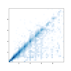
(c) Skylake - Ithemal

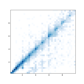
(d) Ivy Bridge - Granite

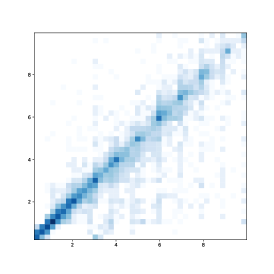
(e) Haswell - Granite

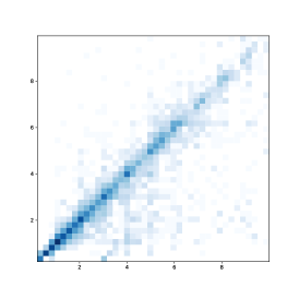
(f) Skylake - Granite

Figure 3: Heatmaps for ground-truth (x axis) and predicted values (y axis) for Ithemal [19] and multi-task Granite learned models on the Ithemal dataset [19] across three different x86-64 microarchitectures for the throughput values under 10 cycles.

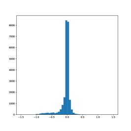
(a) Ivy Bridge - Ithemal

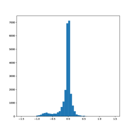
(b) Haswell - Ithemal

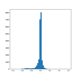
(c) Skylake - Ithemal

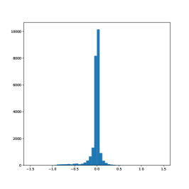
(d) Ivy Bridge - Granite

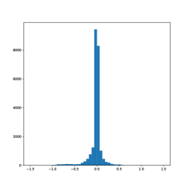
(e) Haswell - Granite

(f) Skylake - Granite

Figure 4: Distribution of relative error (x axis) and the number of basic blocks (y axis) for Ithemal [19] and multi-task Granite learned models on the Ithemal dataset [19] across three different x86-64 microarchitectures, corresponding to heatmaps in Figure 3.

Analysis of learned models on the BHive dataset. Figure 5 illustrates the same analysis for Granite model when trained and tested on the BHive dataset. Note that the Ithemal data set is 5$\times$ bigger than the BHive dataset; hence, the heatmaps in Figure 5 appear to be sparser than heatmaps in Figure 3. Similar to the trend observed in Figure 3, Granite on the BHive dataset yields a comparable performance between underestimated and overestimated predicted values. These detailed analysis of the learned models indicates that Granite consistently outperforms Ithemal [19] across the measured throughput spectrum.

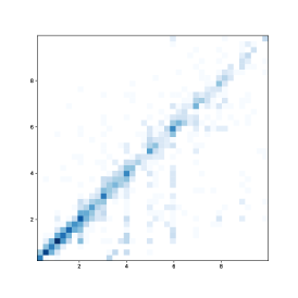
(a) Ivy Bridge - Granite

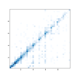
(b) Haswell - Granite

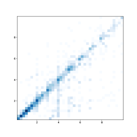
(c) Skylake - Granite

Figure 5: Heatmaps for ground-truth (x axis) and predicted values (y axis) for Ithemal and Granite learned models on the BHive dataset across three different x86-64 microarchitectures for the throughput values under 10 cycles. Note that the BHive [22] dataset contains 5$\times$ less data compared to the Ithemal dataset [19]; Hence the sparser heatmaps.

Table 7: Sensitivity of Granite to the number of message passing iterations on Ithemal dataset [19] across three different microarchitectures.

Microarchitecture	# of Message Passing Iterations	Mean Absolute Error
Ivy Bridge	1	$8.48\%$
	2	$7.85\%$
	4	$7.49\%$
	8	6.67$\%$
	12	$7.30\%$
Haswell	1	$9.42\%$
	2	$9.09\%$
	4	$8.40\%$
	8	7.61$\%$
	12	$8.44\%$
Skylake	1	$8.40\%$
	2	$7.47\%$
	4	$7.05\%$
	8	6.47$\%$
	12	$6.97\%$

5.2 Ablation Studies

In this section, we perform detailed ablation studies across various hyper-parameters of the learned model and summarize our observations.

Sensitivity to the number of message passing iterations. We first sweep the number of message passing iterations in the graph neural network with one, two, four, eight, and twelve. Each message passing iteration constitutes a synchronous exchange of embedding vectors between adjacent graph nodes and edges. The number of message passing iterations limits the distance that information from each node and edge can “travel” in the graph. Increasing the number of iterations allows information exchange between more distant nodes, but at the same time it makes training and inference more computationally expensive.

Table 7 summarizes the results across all three microarchitectures. With eight message passing iterations, Granite achieves the lowest test prediction error, on average, $6.67\%$ and $0.65\%$ lower than Granite with two and six message passing iterations, respectively. The results show that Granite’s performance is indeed sensitive to the number of message passing iterations, suggesting a search to find the sweet spot for this hyper-parameter. We postulate that as the number of nodes (instructions) increases, a higher number of message passing iterations could potentially further reduce the prediction error, owing to better capturing the underlying dependencies between nodes. However, increasing the number of message passing iterations more than a certain value (eight in our setup) could lead to a higher inductive bias to training dataset.

Impact of the decoder network. To determine the effect of the decoder network on the quality of the model, we modified the Ithemal model [19] to use the same multi-layer feed forward network with ReLU non-linearity. We observed that adding the decoder network improved the $\text{Ithemal}^{\textbf{+}}$ model accuracy by $0.25\%$, $0.39\%$, and $1.1\%$ for Ivy Bridge, Haswell, and Skylake, respectively. We attribute these improvement to the additional non-linearity of the decoder network that incorporate more inductive bias to the network. We observe a similar trend in multi-task training, where multi-task learning is most effective in the presence of multi-layer feed forward network. The following provides a possible explanation for this trend. In the vanilla Ithemal model [19], a simple dot-product operation is used to model the throughput computation. We hypothesize that such modeling imposes the task of throughput prediction as well as semantic modeling of basic block dependencies onto LSTM layers, which possibly hinders the capability of the model to construct an expressive representation of basic blocks.

Sensitivity to layer normalization. Layer normalization has proved to be effective in stabilizing the training for recurrent neural networks [34]. As part of the sensitivity study, we explore the impact of layer normalization on Granite accuracy. For this experiment, we remove all the layer normalization from node and edge update networks and the decoder network. The results show that without layer normalization the test prediction error, significantly increases by $15.19\%$, $12.87\%$, and $12.27\%$ for Ivy Bridge, Haswell, and Skylake microarchitectures, respectively. We also observed that disabling layer normalization significantly increases numerical instability that we had to counter by using gradient clipping. This significant increase in the test prediction error suggests the importance of layer normalization in achieving the state-of-the-art accuracy for basic block throughout estimation as well as improving the numerical stability of the training.

Sensitivity to loss function. Finally, we analyze the impact of various loss functions on the final model error. The vanilla Ithemal [19] model trains and evaluates the models using MAPE. However, employing different loss functions may potentially lead to better generalization to unseen data and less overfitting [41]. To verify that MAPE is indeed the best loss function for Granite, we trained the model with other loss functions and evaluated the model MAPE against an equivalent model trained with MAPE. The additional loss functions that we studied are mean squared error (MSE) and Huber loss [42] in two setups: (1) with absolute error, calculated as the difference between predicted and ground-truth values and (2) relative error, computed as the absolute error normalized by the ground-truth value. Compared to MSE, the Huber loss is known to be less sensitive to outliers in the dataset. In all the experiments with Huber loss, we set $\delta$ = 1.

Table 9 summarizes the comparison between different loss function across different microarchitectures. We report various comparison metrics (columns three to six of Table 9) for each loss function. While training with MAPE generally provides best results, we observe that relative MSE may also be a viable option. Other loss functions and in particular loss functions that do not use normalization perform significantly worse due to the high dynamic range of the predicted throughput values.

5.3 Multi-Task Learning

Table 8: The effects of multi-task training on Granite and Ithemal models [19] across different x86-64 microarchitectures.

Microarchitecture	Model	MAPE (Single-Task)	MAPE (Multi-Task)
Ivy Bridge	Ithemal	$8.34\%$	$8.82\%$
	$\text{Ithemal}^{\textbf{+}}$	$8.37\%$	$7.89\%$
	Granite	7.02$\%$	6.67$\%$
Haswell	Ithemal	$9.90\%$	$9.62\%$
	$\text{Ithemal}^{\textbf{+}}$	$8.87\%$	$8.82\%$
	Granite	7.76 $\%$	7.82$\%$
Skylake	Ithemal	$8.30\%$	$8.77\%$
	$\text{Ithemal}^{\textbf{+}}$	$7.65\%$	$7.51\%$
	Granite	7.34 $\%$	6.75 $\%$

In this section, we evaluate the impact of multi-task learning on performance prediction. Each task in this context represents a target microarchitecture (e.g. Ivy Bridge, Haswell, and Skylake). Our goal is to explore whether it is feasible to design a generalized model that works across different microarchitectures, likely with disparate characteristics. When training a multi-task model, we selected basic blocks where we had ground truth data for all target microarchitectures. In addition, for each basic block, we update the weights for all target microarchitectures at the same time.

Table 8 compares the performance of Granite multi-task model and $\text{Ithemal}^{\textbf{+}}$ with multi-task heads. It shows that in most cases using multi-task learning (1) improves the quality of the trained model, and (2) it makes training more efficient by training a single model for multiple microarchitectures at once. The main case where multi-task learning has negative impact on the results is in case of the unmodified Ithemal model [19]. We attribute this to the simplicity of the task-specific decoder part in this model; we see that when the model is augmented with a more complex task-specific decoder, the model can benefit from multi-task training. We also take this as an indication that the shared part of the network learns a representation of code that is sufficiently powerful to support multiple target microarchitectures.

Table 9: Comparison between different loss functions in Granite on Ithemal dataset [19]. Note that in our data sets, throughput values are per 100 iterations of each basic block which explains higher MSE and Huber loss values.

Microarchitecture	Loss Function	MAPE	MSE	Relative MSE	Mean Huber	Mean Relative Huber
Ivy Bridge	MAPE	7.49$\%$	2353023.37	0.926	91.23	0.022
	MSE	$24.94\%$	1709602.44	1.670	124.28	0.072
	Relative MSE	7.72$\%$	1922472.84	0.044	86.85	0.016
	Huber	$10.21\%$	1941646.88	0.966	87.52	0.036
	Relative Huber	$8.34\%$	1702852.03	0.676	88.72	0.022
Haswell	MAPE	8.33$\%$	4883716.03	0.923	146.7	0.024
	MSE	$27.07\%$	16328409.43	2.651	221.21	0.092
	Relative MSE	8.88$\%$	4138913.04	0.056	145.62	0.019
	Huber	$11.51\%$	4175191.19	0.931	142.59	0.039
	Relative Huber	$9.44\%$	3777885.85	0.632	147.65	0.025
Skylake	MAPE	7.32$\%$	1407284.56	0.651	83.52	0.021
	MSE	$26.78\%$	1202691.79	1.570	110.10	0.086
	Relative MSE	7.31$\%$	1282483.60	0.032	80.24	0.013
	Huber	$9.54\%$	820971.73	0.579	66.44	0.029
	Relative Huber	$7.93\%$	1334057.40	0.491	81.31	0.019

5.4 Computational efficiency

Last, we consider the computational efficiency of the models. Efficiency is an important aspect of machine learning models deployed in practical applications. We have evaluated the training and inference throughput of Granite and compared it to the efficiency of other models discussed in this paper. We used a Linux workstation with an Intel Xeon E5-1650-v3 CPU running at 3.50GHz, 128GB RAM, and an NVIDIA RTX 2080 Ti GPU. For training, we report the average time per batch over 300 training steps of each model, whereas for inference, we report the average time per batch on the whole BHive data set of ca 300k basic blocks. In both cases, we used batches of 100 basic blocks.

Table 10 summarizes our results. Overall, we found that Granite is roughly 3x faster than Ithemal and $\text{Ithemal}^{\textbf{+}}$ models both in training an inference when running on a GPU. When running inference on a CPU, Granite is 27% slower. We did not include CPU training time in our evaluation based on the observation that training is virtually always done using GPUs or other accelerators.

Moreover, our measurement have also shown that the overhead of training a multi-task models is negligible compared to training a similar model for a single task both for Granite and models based on the Ithemal architecture. That is, the training cost per microarchitecture of a multi-task model with three heads is almost one third of the cost of training three equivalent single-task models.

Table 10: Run time per batch of 100 blocks of training and inference (in seconds)

Model	Microarchitecture	GPU training	GPU inference	CPU inference
Ithemal single task	Ivy Bridge	0.0996s	0.0491s	0.0551s
	Haswell	0.1236s	0.0501s	0.0558s
	Skylake	0.0775s	0.0502s	0.0556s
Granite single task	Ivy Bridge	0.0354s	0.0147s	0.0749s
	Haswell	0.0367s	0.0147s	0.0750s
	Skylake	0.0349s	0.0146s	0.0751s
$\text{Ithemal}^{\textbf{+}}$ multi-task	Ivy Bridge & Haswell & Skylake	0.1086s	0.0515s	0.0602s
Granite multi-task	Ivy Bridge & Haswell & Skylake	0.0361s	0.0157s	0.0768s

6 Related Work

Granite takes a fundamentally different approach than the prior proposals for performance estimation of basic blocks. In contrast to prior performance estimation work, Granite takes one step further and leverages graph neural network theory to obtain expressive architecture embedding that translates to higher accuracy in the learned models. Below, we overview the most relevant work.

Performance estimation. There is a growing body of work on developing models for performance estimation that can be categorized into analytical models [43, 17, 15, 44, 45, 46, 47, 48, 49, 50, 51, 52, 53, 54, 55, 56] and learning based models [57, 58, 19, 59, 60, 61, 62, 63]. Generally, developing analytical models is an intricate and tedious task in terms of human development, require meticulous understanding of internal microarchitectural details, and are rarely generalizable to different architectures. In contrast, Granite is a learning based model that aims to mitigate these challenges by leveraging machine learning techniques.

In the learned model category, Ithemal [19] is the closest work to this paper in terms of overall approach. Ithemal uses a sequential LSTM-based model in which only the structural dependencies between adjacent instructions are present in an explicit form. In contrast, Granite uses GNNs to capture both short- and long-range dependencies between instructions in a graph representation of the basic block. In addition, this work takes one step further and, for the first time to the best of our knowledge, presents multi-task learning [21] for throughput estimation across different architectures. Kaufman et al. [57] introduce a GNN-based performance model for tensor computation graphs on TPUs [64]. While tensor computation kernels are more complex than straight-line code like basic blocks, the in-order execution model of TPUs and the lack of hardware caching simplifies the task significantly. In contrast, Granite targets throughout prediction in architectures with complex out-of-order execution models and multi-level caching.

Graph neural networks. There is a growing interest of using graph neural networks in various reasoning tasks and to construct expressive low-dimensional representations from graph structures [28, 65, 66, 67, 68, 69, 70, 71, 71, 72, 73]. These learned low-dimensional representations are then generally processed to estimate desired metrics. Computer programs can be represented naturally as graphs in which the nodes are associated with different elements of the assembly language representation of the code and the edges model different dependencies between these elements. Recent work [74, 20, 75, 76] explores the idea of constructing graphs from source code and shows the strength of graph neural networks in various prediction tasks. As a natural step, we also use graphs to represent the dependencies in basic blocks and leverages the recent progress in graph neural networks [67] to construct expressive representations for throughput estimation.

7 Conclusion

We present Granite, a graph neural network model that establishes the state-of-the-art model accuracy for throughput estimation of basic blocks across various x86-64 microarchitectures. Our results show that Granite estimates the throughput of basic blocks with average test error of 6.91$\%$ across different microarchitectures, 1.7$\%$ over the previous state-of-the-art model [19], while also achieving  3x higher throughput in training and inference, which can be further multiplied by training a single model to predict throughput for multiple target microarchitectures at the same time. We have achieved these results by bringing in ideas from other fields of machine learning, such as graph neural networks [28] and multi-task learning [21].

These promising results reinforce our claim about the expressiveness of the low-dimensional representations of basic blocks using graph neural networks. We argue that using graphs to represent programs not only leads to richer low-dimensional representations which translate to higher accuracy and better generalization, but also paves the way to associate low-level microarchitectural features, such as performance counters, to each instruction. This relational association between low-level microarchitectural features and programs is an exciting future research direction.

References

- [1] R. C. Lozano, M. Carlsson, F. Drejhammar, and C. Schulte, “Constraint-based Register Allocation and Instruction Scheduling,” in CP, 2012.
- [2] M. Stephenson, S. Amarasinghe, M. Martin, and U.-M. O’Reilly, “Meta Optimization: Improving Compiler Heuristics with Machine Learning,” ACM sigplan notices, 2003.
- [3] A. McGovern and J. E. B. Moss, “Scheduling Straight-line Code Using Reinforcement Learning and Rollouts,” in NeurIPS, 1999.
- [4] D. Nuzman and A. Zaks, “Autovectorization in GCC–Two Years Later,” in GCC Developers Summit, 2006.
- [5] Z. Jia, J. Thomas, T. Warszawski, M. Gao, M. Zaharia, and A. Aiken, “Optimizing DNN Computation with Relaxed Graph Substitutions,” SysML, 2019.
- [6] D. Narayanan, A. Harlap, A. Phanishayee, V. Seshadri, N. R. Devanur, G. R. Ganger, P. B. Gibbons, and M. Zaharia, “PipeDream: Generalized Pipeline Parallelism for DNN Training,” in SOSP, 2019.
- [7] D. Narayanan, K. Santhanam, F. Kazhamiaka, A. Phanishayee, and M. Zaharia, “Heterogeneity-Aware Cluster Scheduling Policies for Deep Learning Workloads,” in OSDI, 2020.
- [8] M. Trofin, Y. Qian, E. Brevdo, Z. Lin, K. Choromanski, and D. Li, “MLGO: A Machine Learning Guided Compiler Optimizations Framework,” arXiv preprint arXiv:2101.04808, 2021.
- [9] T. Gysi, T. Grosser, and T. Hoefler, “Absinthe: Learning an Analytical Performance Model to Fuse and Tile Stencil Codes in One Shot,” in PACT, 2019.
- [10] A. Yazdanbakhsh, C. Angermueller, B. Akin, Y. Zhou, A. Jones, M. Hashemi, K. Swersky, S. Chatterjee, R. Narayanaswami, and J. Laudon, “Apollo: Transferable Architecture Exploration,” arXiv preprint arXiv:2102.01723, 2021.
- [11] Y. Zhou, X. Dong, T. Meng, M. Tan, B. Akin, D. Peng, A. Yazdanbakhsh, D. Huang, R. Narayanaswami, and J. Laudon, “Towards the Co-design of Neural Networks and Accelerators,” MLSys, 2022.
- [12] K. Hegde, P.-A. Tsai, S. Huang, V. Chandra, A. Parashar, and C. W. Fletcher, “Mind Mappings: Enabling Efficient Algorithm-Accelerator Mapping Space Search,” in ASPLOS, 2021.
- [13] A. Kumar, A. Yazdanbakhsh, M. Hashemi, K. Swersky, and S. Levine, “Data-Driven Offline Optimization For Architecting Hardware Accelerators,” ICLR, 2022.
- [14] J. Laukemann, J. Hammer, G. Hager, and G. Wellein, “Automatic Throughput and Critical Path Analysis of x86 and ARM Assembly Kernels,” in PMBS, 2019.
- [15] A. D. Biagio and M. Davis, “LLVM Machine Code Analyzer,” https://llvm.org/docs/CommandGuide/llvm-mca.html, 2019, accessed: 2020-09-10.
- [16] C. Courbet and G. Chatelet, “Static Execution Performance Analysis with LLVM,” https://github.com/google/EXEgesis/tree/master/llvm_sim, 2020, accessed: 2020-09-10.
- [17] I. Corporation, “Intel Architecture Code Analyzer,” https://software.intel.com/content/www/us/en/develop/articles/intel-architecture-code-analyzer.html, 2019, accessed: 2020-09-10.
- [18] A. Abel and J. Reineke, “UiCA: Accurate Throughput Prediction of Basic Blocks on Recent Intel Microarchitectures,” in ICS, 2022.
- [19] C. Mendis, A. Renda, S. P. Amarasinghe, and M. Carbin, “Ithemal: Accurate, Portable and Fast Basic Block Throughput Estimation using Deep Neural Networks,” in ICML, 2019.
- [20] Z. Shi, K. Swersky, D. Tarlow, P. Ranganathan, and M. Hashemi, “Learning Execution through Neural Code Fusion,” in ICLR, 2019.
- [21] R. Caruana, “Multitask Learning,” Machine Learning, 1997.
- [22] Y. Chen, A. Brahmakshatriya, C. Mendis, A. Renda, E. Atkinson, O. Sỳkora, S. Amarasinghe, and M. Carbin, “BHive: A Benchmark Suite and Measurement Framework for Validating x86-64 Basic Block Performance Models,” in IISWC, 2019.
- [23] S. Hochreiter and J. Schmidhuber, “Long Short-term Memory,” Neural computation, 1997.
- [24] M. Gori, G. Monfardini, and F. Scarselli, “A New Model for Learning in Graph Domains,” in IJCNN, 2005.
- [25] F. Scarselli, S. L. Yong, M. Gori, M. Hagenbuchner, A. C. Tsoi, and M. Maggini, “Graph Neural Networks for Ranking Web Pages,” in WI, 2005.
- [26] T. N. Kipf and M. Welling, “Semi-supervised Classification with Graph Convolutional Networks,” arXiv preprint arXiv:1609.02907, 2016.
- [27] Z. Wu, S. Pan, F. Chen, G. Long, C. Zhang, and S. Y. Philip, “A Comprehensive Survey on Graph Neural Networks,” IEEE Transactions on Neural Networks and Learning Systems, 2020.
- [28] P. W. Battaglia, J. B. Hamrick, V. Bapst, A. Sanchez-Gonzalez, V. Zambaldi, M. Malinowski, A. Tacchetti, D. Raposo, A. Santoro, R. Faulkner, C. Gulcehre, F. Song, A. Ballard, J. Gilmer, G. Dahl, A. Vaswani, K. Allen, C. Nash, V. Langston, C. Dyer, N. Heess, D. Wierstra, P. Kohli, M. Botvinick, O. Vinyals, Y. Li, and R. Pascanu, “Relational Inductive Biases, Deep Learning, and Graph Networks,” arXiv preprint arXiv:1806.01261, 2018.
- [29] N. Park, A. Kan, X. L. Dong, T. Zhao, and C. Faloutsos, “Estimating Node Importance in Knowledge Graphs using Graph Neural Networks,” in KDD, 2019.
- [30] A. LeClair, S. Haque, L. Wu, and C. McMillan, “Improved Code Summarization via a Graph Neural Network,” arXiv preprint arXiv:2004.02843, 2020.
- [31] J. Gilmer, S. S. Schoenholz, P. F. Riley, O. Vinyals, and G. E. Dahl, “Neural Message Passing for Quantum Chemistry,” arXiv preprint arXiv:1704.01212, 2017.
- [32] M. Bajaj, L. Wang, and L. Sigal, “G3raphGround: Graph-Based Language Grounding,” in ICCV, 2019.
- [33] K. He, X. Zhang, S. Ren, and J. Sun, “Deep residual learning for image recognition,” in Proceedings of the IEEE Conference on Computer Vision and Pattern Recognition (CVPR), June 2016.
- [34] J. L. Ba, J. R. Kiros, and G. E. Hinton, “Layer Normalization,” arXiv preprint arXiv:1607.06450, 2016.
- [35] C. Lattner and V. Adve, “LLVM: A Compilation Framework for Lifelong Program Analysis & Transformation,” in CGO, 2004.
- [36] SPEC, “SPEC CPU®2006,” https://www.spec.org/cpu2006/, 2006, accessed: 2022-07-06.
- [37] ——, “SPEC CPU®2017,” https://www.spec.org/cpu2017/, 2017, accessed: 2022-07-06.
- [38] M. Abadi, A. Agarwal, P. Barham, E. Brevdo, Z. Chen, C. Citro, G. S. Corrado, A. Davis, J. Dean, M. Devin, S. Ghemawat, I. Goodfellow, A. Harp, G. Irving, M. Isard, Y. Jia, R. Jozefowicz, L. Kaiser, M. Kudlur, J. Levenberg, D. Mané, R. Monga, S. Moore, D. Murray, C. Olah, M. Schuster, J. Shlens, B. Steiner, I. Sutskever, K. Talwar, P. Tucker, V. Vanhoucke, V. Vasudevan, F. Viégas, O. Vinyals, P. Warden, M. Wattenberg, M. Wicke, Y. Yu, and X. Zheng, “TensorFlow: Large-Scale Machine Learning on Heterogeneous Systems,” 2015, software available from tensorflow.org. [Online]. Available: http://tensorflow.org/
- [39] “Graph Nets Library,” https://github.com/deepmind/graph_nets, 2020.
- [40] D. P. Kingma and J. Ba, “Adam: A Method for Stochastic Optimization,” arXiv preprint arXiv:1412.6980, 2014.
- [41] H. Li, Z. Xu, G. Taylor, C. Studer, and T. Goldstein, “Visualizing the Loss Landscape of Neural Nets,” NeurIPS, 2018.
- [42] P. J. Huber, “Robust Estimation of a Location Parameter,” in Breakthroughs in statistics, 1992.
- [43] J. Laukemann, J. Hammer, G. Hager, and G. Wellein, “Automatic Throughput and Critical Path Analysis of x86 and ARM Assembly Kernels,” in PMBS, 2019.
- [44] J. Laukemann, J. Hammer, J. Hofmann, G. Hager, and G. Wellein, “Automated Instruction Stream Throughput Prediction for Intel and AMD Microarchitectures,” in PMBS, 2018.
- [45] D. Sanchez and C. Kozyrakis, “ZSim: Fast and Accurate Microarchitectural Simulation of Thousand-core Systems,” ACM SIGARCH Computer architecture news, 2013.
- [46] A. Patel, F. Afram, S. Chen, and K. Ghose, “MARSS: A Full System Simulator for Multicore x86 CPUs,” in DAC, 2011.
- [47] X. E. Chen and T. M. Aamodt, “A First-order Fine-grained Multithreaded Throughput Model,” in HPCA, 2009.
- [48] T. M. Taha and S. Wills, “An Instruction Throughput Model of Superscalar Processors,” IEEE Transactions on Computers, 2008.
- [49] X. Li, Y. Liang, T. Mitra, and A. Roychoudhury, “Chronos: A Timing Analyzer for Embedded Software,” Science of Computer Programming, 2007.
- [50] V. S. Adve and M. K. Vernon, “Parallel Program Performance Prediction using Deterministic Task Graph Analysis,” TOCS, 2004.
- [51] V. Blanco, J. A. González, C. León, C. Rodrıguez, G. Rodrıguez, and M. Printista, “Predicting the Performance of Parallel Programs,” Parallel Computing, 2004.
- [52] C. Ferdinand, R. Heckmann, M. Langenbach, F. Martin, M. Schmidt, H. Theiling, S. Thesing, and R. Wilhelm, “Reliable and Precise WCET Determination for a Real-life Processor,” in International Workshop on Embedded Software, 2001.
- [53] R. Rugina and K. E. Schauser, “Predicting the Running Times of Parallel Programs by Simulation,” in IPDPS, 1998.
- [54] T. Fahringer and H. P. Zima, “A Static Parameter based Performance Prediction Tool for Parallel Programs,” in ICS, 1993.
- [55] C. Y. Park, “Predicting Program Execution Times by Analyzing Static and Dynamic Program Paths,” Real-Time Systems, 1993.
- [56] F. Hartleb and V. Mertsiotakis, “Bounds for the Mean Runtime of Parallel Programs,” in Proceedings of the Sixth International Conference on Modelling Techniques and Tools for Computer Performance Evaluation, 1992.
- [57] S. Kaufman, P. Phothilimthana, Y. Zhou, C. Mendis, S. Roy, A. Sabne, and M. Burrows, “A Learned Performance Model for Tensor Processing Units,” MLSys, 2021.
- [58] A. Adams, K. Ma, L. Anderson, R. Baghdadi, T.-M. Li, M. Gharbi, B. Steiner, S. Johnson, K. Fatahalian, F. Durand, and J. Ragan-Kelley, “Learning to Optimize Halide with Tree Search and Random Programs,” TOG, 2019.
- [59] S. A. Seshia and A. Rakhlin, “Quantitative Analysis of Systems using Game-theoretic Learning,” TECS, 2012.
- [60] S. A. Seshia and J. Kotker, “GameTime: A Toolkit for Timing Analysis of Software,” in TACAS, 2011.
- [61] L. Huang, J. Jia, B. Yu, B.-G. Chun, P. Maniatis, and M. Naik, “Predicting Execution Time of Computer Programs using Sparse Polynomial Regression,” in NeurIPS, 2010.
- [62] C. Dubach, J. Cavazos, B. Franke, G. Fursin, M. F. O’Boyle, and O. Temam, “Fast Compiler Optimisation Evaluation using Code-feature based Performance Prediction,” in CF, 2007.
- [63] K. Seshadri, B. Akin, J. Laudon, R. Narayanaswami, and A. Yazdanbakhsh, “An Evaluation of Edge TPU Accelerators for Convolutional Neural Networks,” in IISWC, 2022.
- [64] N. P. Jouppi, C. Young, N. Patil, D. Patterson, G. Agrawal, R. Bajwa, S. Bates, S. Bhatia, N. Boden, A. Borchers, R. Boyle, P.-l. Cantin, C. Chao, C. Clark, J. Coriell, M. Daley, M. Dau, J. Dean, B. Gelb, T. V. Ghaemmaghami, R. Gottipati, W. Gulland, R. Hagmann, C. R. Ho, D. Hogberg, J. Hu, R. Hundt, D. Hurt, J. Ibarz, A. Jaffey, A. Jaworski, A. Kaplan, H. Khaitan, A. Koch, N. Kumar, S. Lacy, J. Laudon, J. Law, D. Le, C. Leary, Z. Liu, K. Lucke, A. Lundin, G. MacKean, A. Maggiore, M. Mahony, K. Miller, R. Nagarajan, R. Narayanaswami, R. Ni, K. Nix, T. Norrie, M. Omernick, N. Penukonda, A. Phelps, J. Ross, M. Ross, A. Salek, E. Samadiani, C. Severn, G. Sizikov, M. Snelham, J. Souter, D. Steinberg, A. Swing, M. Tan, G. Thorson, B. Tian, H. Toma, E. Tuttle, V. Vasudevan, R. Walter, W. Wang, E. Wilcox, and D. H. Yoon, “In-Datacenter Performance Analysis of a Tensor Processing Unit,” in ISCA, 2017.
- [65] D. Beck, G. Haffari, and T. Cohn, “Graph-to-Sequence Learning using Gated Graph Neural Networks,” arXiv preprint arXiv:1806.09835, 2018.
- [66] T. H. Nguyen and R. Grishman, “Graph Convolutional Networks With Argument-Aware Pooling for Event Detection,” in AAAI, 2018.
- [67] J. Zhou, G. Cui, Z. Zhang, C. Yang, Z. Liu, L. Wang, C. Li, and M. Sun, “Graph Neural Networks: A Review of Methods and Applications,” arXiv preprint arXiv:1812.08434, 2018.
- [68] D. Marcheggiani, J. Bastings, and I. Titov, “Exploiting Semantics in Neural Machine Translation with Graph Convolutional Networks,” arXiv preprint arXiv:1804.08313, 2018.
- [69] J. Bastings, I. Titov, W. Aziz, D. Marcheggiani, and K. Sima’an, “Graph Convolutional Encoders for Syntax-aware Neural Machine Translation,” arXiv preprint arXiv:1704.04675, 2017.
- [70] A. Santoro, D. Raposo, D. G. Barrett, M. Malinowski, R. Pascanu, P. Battaglia, and T. Lillicrap, “A Simple Neural Network Module for Relational Reasoning,” in NeurIPS, 2017.
- [71] N. Peng, H. Poon, C. Quirk, K. Toutanova, and W.-t. Yih, “Cross-Sentence N-ary Relation Extraction with Graph LSTMs,” TACL, 2017.
- [72] M. Miwa and M. Bansal, “End-to-end Relation Extraction using LSTMs on Sequences and Tree Structures,” arXiv preprint arXiv:1601.00770, 2016.
- [73] P. Battaglia, R. Pascanu, M. Lai, D. J. Rezende, and K. Kavukcuoglu, “Interaction Networks for Learning about Objects, Relations and Physics,” in NeurIPS, 2016.
- [74] U. Alon, M. Zilberstein, O. Levy, and E. Yahav, “code2vec: Learning Distributed Representations of Code,” POPL, 2019.
- [75] M. Allamanis, M. Brockschmidt, and M. Khademi, “Learning to Represent Programs with Graphs,” arXiv preprint arXiv:1711.00740, 2017.
- [76] C. Cummins, Z. V. Fisches, T. Ben-Nun, T. Hoefler, and H. Leather, “ProGraML: Graph-based Deep Learning for Program Optimization and Analysis,” arXiv preprint arXiv:2003.10536, 2020.