Hybrid Simulator for Space Docking and Robotic Proximity Operations

Abstract

In this work, we present a hybrid simulator for space docking and robotic proximity operations methodology. This methodology also allows for the emulation of a target robot operating in a complex environment by using an actual robot. The emulation scheme aims to replicate the dynamic behavior of the target robot interacting with the environment, without dealing with a complex calculation of the contact dynamics. This method forms a basis for the task verification of a flexible space robot. The actual emulating robot is structurally rigid, while the target robot can represent any class of robots, e.g., flexible, redundant, or space robots. Although the emulating robot is not dynamically equivalent to the target robot, the dynamical similarity can be achieved by using a control law developed herein. The effect of disturbances and actuator dynamics on the fidelity and the contact stability of the robot emulation is thoroughly analyzed.

1 Introduction and Motivation

There is growing interest in employing robotic manipulators to perform assembly tasks. In particular, space robots have become a viable means to perform extra-vehicular robotic tasks [1, 2, 3, 4, 5, 6, 7, 8, 9, 10]. For instance, the Special Purpose Dextrous Manipulator (SPDM) will be used to handle various orbital replacement units (ORU) for maintenance operations performed on the International Space Station.

The complexity of a robotic operation associated with a task demands a verification facility on the ground to ensure that the task can be performed on orbit as intended. This requirement has motivated the development of the SPDM task verification facility at Canadian Space Agency [11, 12, 13, 14, 15, 16, 7]. The verification operation on the ground is challenging as space robots are designed to work only in a micro-g environment. Actually, thanks to weightlessness on orbit, the SPDM can handle payloads as massive as $600\;kg$. On the ground, however, it cannot even support itself against gravity. Although this problem could be fixed by using a system of weights and pullies to counterbalance gravity, the weights change the robot inertia and its dynamic behavior. Moreover, it is difficult to replicate the dynamic effects induced by the flexibility of the space robot or space structure on which the manipulator is stowed.

Simulation is another tool that can be used to validate the functionality of a space manipulator [17]. Although the dynamics and kinematics models of space manipulators are more complex that those of terrestrial manipulators due to dynamic coupling between the manipulator and its spacecraft, Vafa et al. [18, 19] showed that the space-robot dynamics can be captured by the concept of a Virtual-Manipulator, which has a fixed base in inertial space at a point called Virtual Ground. Today, with the advent of powerful computers, faithful and real-time simulators exist, which are able to capture dynamics of almost any type of manipulator with many degrees of freedom. However, simulation of a robot interacting with its environment with a high fidelity requires accurate modelling of both the manipulator and the contact interface between the manipulator and its environment. Faithful models of space-robots are available; it is the calculation of the contact force which poses many technical difficulties associated with contact dynamics [20]. In the literature, many models for the contact force, comprised of normal and friction forces, have been reported [21, 20, 22]. Hertzian contact theory is used to estimate local forces [22]. However, predicting the contact point locations requires calling an optimization routine [20], thus demanding substantial computational effort. In particular, the complexity of contact-dynamics modelling tends to increase exponentially when the two objects have multi-point contacts [17]. Moreover, since the SPDM is tele-operated by a human operator, the validation process requires inclusion of a real-time simulation environment since the simulation should allow human operators to drive the simulation in real-time. All these difficulties can be avoided by emulating the contact dynamics.

Figure 1: Schematics of the space manipulator (A) and the terrestrial manipulator (B) performing a task involving contact.

Design and implementation of a laboratory test-bed for study the dynamics coupling between a space-manipulator and its spacecraft operating in free space are presented in [23]. Similar concepts have been also pursued by other space agencies for different applications [24, 25, 26, 27, 28, 29, 30, 31, 32, 33, 34, 35, 34, 36]. In this work we develop an emulation technique which can replicate the dynamic behavior of a robot interacting with a complex environment, without actually simulating the environment [1]. Fig.1B schematically illustrates the concept of the robot emulation system. The system consists of three main functional elements: a real-time simulator capturing the dynamics of the space robot, the mock-up of the payload and its work-site, and a rigid robot which handles the payload. Interconnecting the simulator and the emulating robot, the entire system works in a hardware-in-loop simulation configuration that permits us to replicate the dynamic behavior of the space robot [1, 12, 7].

The purpose of the control system is to make the constrained-motion dynamical behavior of the emulating robot as close as possible to that actually encountered by the space robot [1]. The obvious advantage of this methodology is that there is no need for modeling a complex environment. Moreover, because of using the real hardware, a visual cue of the payload and the work-site is available which otherwise, must be simulated. The main contribution of this paper is to layout a control architecture for the emulation of a robot operating in free space and in contact with the environment. It follows by an analysis of the fidelity and the stability of the robot emulation; the validity of the analysis is demonstrated by experimental results.

This paper is organized as follows: In section 2, we formulate the emulation problem and develop the control law. Section 3 describes the equations of motion of independent coordinate which arise in the case of flexible target robots. A thorough analysis of the robot emulation, including fidelity of the emulation with respect to the disturbance and stability conditions are given in section 4.

2 Control of Emulating Robot

Let’s consider an emulating robot and a target robot, referred to by subscripts $r$ and $s$, with $n$ and $m$ degrees-of-freedom (DOF), respectively, operating in an $n$-dimensional task space. The generalized coordinates of the robots are represented by vectors $q_{r}\in\mathbb{R}^{n}$ and $q_{s}\in\mathbb{R}^{m}$, respectively. Note that the emulating robot is rigid but the space robot is typically a flexible one with many degrees-of-freedom. Hence, we can say

$$\mbox{dim}(q_{s})=m\geq\mbox{dim}(q_{r})=n.$$

Let vector $p_{r}^{T}=[x_{r}^{T},\phi_{r}^{T}]$ denote the pose of the end-effector of the emulating robot, where $x_{r}$ and $\phi_{r}$ describe, respectively, the position and a minimal representation of the orientation of the end-effector expressed in the base frame attached to the work-site; see Fig.1. Similarly, the pose of the target robot is denoted by vector $p_{s}$.

Assumption 1

1. Both robots have identical end-effector pose configuration with respect to their base frames, i.e., $p_{r}=p_{s}=p$ and

2. they experience the same contact force/moment $f\in\mathbb{R}^{n}$.

Moreover, we assume that $M_{r}\in\mathbb{R}^{n\times n}$ and $M_{s}\in\mathbb{R}^{m\times m}$ are the inertia matrices of the two manipulators; $h_{r}\in\mathbb{R}^{n}$ and $h_{r}\in\mathbb{R}^{m}$ contain Coriolis, centrifugal, friction, gravity (for the emulating robot), and stiffness (for the space robot); $\tau_{r}\in\mathbb{R}^{n}$ and $\tau_{s}\in\mathbb{R}^{n}$ are the joint torque vectors; and that $J_{r}=\partial p_{r}/\partial q_{r}\in\mathbb{R}^{n\times n}$ and $J_{s}=\partial p_{s}/\partial q_{s}\in\mathbb{R}^{n\times m}$ are the analytical Jacobian matrices. Then, the equations of motion of the robots can be described by [37, 38, 39]

$$M_{r}\ddot{q}_{r}+h_{r}(q_{r},\dot{q}_{r})=\tau_{r}+J_{r}^{T}f_{a},$$ (1)

$$M_{s}\ddot{q}_{s}+h_{s}(q_{s},\dot{q}_{s})=B\tau_{s}+J_{s}^{T}f_{a},$$ (2)

where $B=\left[\begin{array}[]{c}I\\ 0\end{array}\right]\in\mathbb{R}^{m\times n}$, and $f_{a}\in\mathbb{R}^{n}$ is the vector of generalized constraint force expressed in the base frame. Note that $f_{a}$ performs work on $\dot{p}$, and it is related to the contact force $f$ by

$$f_{a}=\Lambda(\phi)f,$$ (3)

where $\Lambda(\phi)=\mbox{diag}\{I,\Lambda_{1}(\phi)\}$ is a transformation matrix that depends on a particular set of parameters used to represent the end-effector orientation [37]; $\phi_{s}=\phi_{r}=\phi$ because of Assumption 1.

Now, assume that a real-time simulator captures the dynamics of the space robot. Also, assume that the endpoint pose of the simulated robot is constrained by that of the emulating robot, i.e., the following rheonomic constraint

$${\Phi}({q}_{s},{q}_{r}(t))=p_{r}(q_{r}(t))-p_{s}(q_{s})\equiv 0$$ (4)

holds. Enforcing the constraint ensures that the end-effector of the simulated robot is constrained by the pose of the environment barriers, which physically constrains the emulating robot [40, 41, 42]. The Lagrange equations of the simulated robot can be formally expressed by a set of Differential Algebraic Equations (DAE) as

$$M_{s}\ddot{q}_{s}+{\Phi}_{q_{s}}^{T}\lambda=-h_{s}+B\tau_{s}.$$ (5)

$${\Phi}(q_{s},t)=0$$ (6)

where ${\Phi}_{qs}=\partial{\Phi}/\partial q_{s}=-J_{s}\in\mathbb{R}^{m\times n}$ denotes the Jacobian of the constraint with respect to $q_{s}$, and $\lambda\in\mathbb{R}^{n}$ represents the Lagrange multiplier which can be solved from equation (5) together with the second time derivative of the constraint equation (6). That is,

$${\lambda}=(J_{s}M_{s}^{-1}{J}_{s}^{T})^{-1}\left(c+J_{s}M_{s}^{-1}(h_{s}-B\tau_{s})\right),$$ (7)

where $c=\ddot{p}_{r}(t)-\dot{J}_{s}\dot{q}_{s}$; note that the constraint force $\lambda$ can be measured only if a measurement of pose acceleration $\ddot{p}_{r}$ is available, say via an accelerometer.

A comparison of equations (5) and (2) reveals that the Lagrange multiplier ${\lambda}$ acts as a constraint force/moment on the simulated robot. Therefore, our goal is to equate the constraint force and the Lagrange multiplier, i.e., $f_{a}={\lambda}$. This can be achieved by using the computed torque method in the task space [38, 43, 37, 31, 44]. Substituting the joint acceleration from (1) into the second time derivative of the pose, $\ddot{p}_{r}=J_{r}\ddot{q}_{r}+\dot{J}_{r}\dot{q}_{r}$, yields

$$\ddot{p}_{r}=J_{r}M_{r}^{-1}(\tau_{r}+J_{r}^{T}f_{a}-h_{r})+\dot{J}_{r}\dot{q}_{r}.$$ (8)

This equation can then be substituted into (7) to obtain the joint torque solution, assuming $f_{a}=\lambda$. That is

$$\tau_{r}^{c} = h_{r}+M_{r}J_{r}^{-1}(J_{s}M_{s}^{-1}(B\tau_{s}-h_{s})+\dot{J}_{s}\dot{q}_{s}-\dot{J}_{r}\dot{q}_{r})$$ (9)

$$-\underbrace{J_{r}^{T}(I-{\cal M}_{r}{\cal M}_{s}^{-1})f_{a}}_{\mbox{force feedback}},$$

where ${\cal M}:=\left[JM^{-1}J^{T}\right]^{-1}$ is the Cartesian inertia matrix whose inverse can be interpreted as mechanical impedance. The torque control (9) can be grouped into force and motion feedback terms.

Remark 1

The force feedback gain tends to decrease when the inertia ratio approaches one. In the limit, i.e., when ${\cal M}_{s}={\cal M}_{r}$, the force feedback is disabled, and hence the robot emulation can be realized without using force feedback.

In free space, where $f_{a}=0$, the controller matches the end-point poses of two robots at acceleration level and that inevitably leads to drift. We can improve the control law by incorporating a feedback loop to minimize the drift error, i.e.,

$$\tau_{r}^{c} = h_{r}-M_{r}J_{r}^{-1}\dot{J}_{r}\dot{q}_{r}-J_{r}^{T}f_{r}+M_{r}J_{r}^{-1}u$$ (10)

where

$$u:=\tilde{a}_{s}-G_{v}(J_{r}\dot{q}_{r}-\int\tilde{a}_{s}dt)-G_{p}(p_{r}(q_{r})-\int\int\tilde{a}_{s}dt)$$ (11)

is the auxiliary input, $\tilde{a}_{s}:=J_{s}M_{s}^{-1}(B\tau_{s}-h_{s})+\dot{J}_{s}\dot{q}_{s}+J_{s}M_{s}^{-1}J_{s}^{T}f_{a}$ is the estimated pose acceleration of the target robot calculated from the unconstrained dynamics model, and $G_{v}>0$ and $G_{p}>0$ are drift compensation gains. In the following, we show that the constraint force asymptotically tracks the Lagrange multiplier. Denoting

$$\ddot{e}_{p}:=\ddot{p}_{r}-\tilde{a}_{s},$$

then the dynamics of the errors under the control law (10) is

$$\ddot{e}_{p}+G_{v}\dot{e}_{p}+G_{p}e_{p}=0.$$ (12)

The dynamics is asymptotically stable if the gain parameters are adequately chosen, i.e., $e_{p},\dot{e}_{p},\ddot{e}_{p}\rightarrow 0$ as $t\rightarrow\infty$. Furthermore, let

$$e_{f}:=f_{a}-\lambda,$$ (13)

represent the force error. Then, one can show from (7) that the force error is related to the acceleration error by

$$e_{f}={\cal M}_{s}\ddot{e}_{p}.$$ (14)

Since the mass matrix is bounded, i.e. $\exists\kappa>0$ such that ${\cal M}_{s}(q_{s})\leq\kappa I$, then

$$\|e_{f}\|\leq\kappa\|\ddot{e}_{p}\|$$

and hence $e_{f}\rightarrow 0$ as $t\rightarrow\infty$. Therefore, the error between the constraint force and the Lagrange multiplier is asymptotically stable under the control law (10). The above mathematical development can be summarized in the following proposition.

Proposition 1

Assuming the following: (i) the endpoint pose of the simulated robot is constrained with that of the emulating robot performing a contact task, (ii) the torque control law (10) is applied on the emulating robot. Then, (i) the emulating robot produces the end-effector motion of the space robot, (ii) the constraint force asymptotically approaches the Lagrange multiplier: $f_{a}\rightarrow\lambda$.

In this case, the simulated robot behaves as if it interacts virtually with the same environment as the emulating robot does. In other words, the combined system of the simulator and the emulating robot is dynamically equivalent to the original target robot.

2.1 Force Error Feedback

Incorporating a feedback of the force error into the control law (10)-(11) can improve the force response of the emulating system, particularly during the non-contact to contact transition. However, to establish such a feedback requires an estimation of the force error, which, in turn, can be obtained from (14) provided that a measurement of the pose acceleration is available. Then one can show that changing the auxiliary input (11) to $u=\tilde{a}_{s}-G_{v}\dot{e}_{p}-G_{p}e_{p}-G_{f}e_{f}$, where $G_{f}>0$ is the force feedback gain, yields the following error dynamics

$$[I+{\cal M}_{s}G_{f}]\ddot{e}_{p}+G_{v}\dot{e}_{p}+G_{p}e_{p}=0.$$

The above differential equation is asymptotically stable if the force feedback gain is sufficiently small— see Appendix A.

3 Calculating States of the Flexible Robot

To implement control law (10) the values of $q_{r}$, $q_{s}$, and their time derivatives are required. Vectors $q_{r}$ and $\dot{q}_{r}$ can be measured, but $q_{s}$ and its time derivative should be obtained by calculation. Consider the rheonomic constraint ${\Phi}(q_{r}(t),q_{s})=0$ whose differentiation with respect to time leads to

$$J_{s}\dot{q}_{s}=J_{r}\dot{q}_{r}(t)=\dot{p}_{r}(t)$$ (15)

In the case that both robots have the same number of degrees of freedom, i.e., $m=n$, one can obtain $\dot{q}_{s}$ uniquely from the above equation. Subsequently, $q_{s}$ can be found algebraically through solving inverse kinematics $\Phi(q_{r}(t),q_{s})=0$, that is $q_{s}=\Omega(q_{r}(t))$. Although, more often an explicit function may not exist, one can solve the set of nonlinear constraint equations numerically, e.g., by using the Newton-Raphson method, as elaborated in Appendix B. Alternatively, an estimation of $q_{s}$, can be solved by resorting to a closed-loop inverse kinematic (CLIK) scheme based on either the Jacobian transpose [45, 46] or the Jacobian pseudoinverse [47].

Figure 2: The CLIK jacobian transpose scheme for extracting the generalized coordinate of the target manipulator.

Since the emulating robot is structurally rigid while the simulated robot is usually flexible, we can say $n<m$. Therefore, there are less equations than unknowns in (15). The theory of linear systems equations establishes [48] that the general solution can be expressed by

$$\dot{q}_{s}=\dot{q}_{s}^{p}+P\xi,$$ (16)

where

$$\dot{q}_{s}^{p}:=J_{s}^{+}\dot{p}_{r}(t)=J_{s}^{+}J_{r}\dot{q}_{r}(t).$$ (17)

is the particular solution and $P\xi$ represents the general solution of the homogenous velocity. In the above $J_{s}^{+}=J_{s}^{T}(J_{s}J_{s}^{T})^{-1}$ is the pseudoinverse of $J_{s}$, and $P$ is a projection matrix whose columns annihilate the constraints [48], i.e., $J_{s}P=0$, and $\xi\in\mathbb{R}^{n-m}$ is the independent coordinate, which represents the self-motion of the robot.

Similarly, the general solution of acceleration can be found from the second derivative of the constraint equations as

$$\ddot{q}_{s}=P\dot{\xi}+J_{s}^{+}c$$ (18)

with $c$ defined previously below (7). Now, substituting the acceleration from (18) into (5) and premultiplying by $P^{T}$ and knowing that that $P^{T}$ annihilates the constraint force, i.e., $P^{T}J_{s}^{T}=0$, we arrive at

$$N\dot{\xi}=P^{T}h_{s}+v,$$ (19)

where $N=P^{T}M_{s}P$ and $v=P^{T}M_{s}J_{s}^{+}c$. Equation (19) expresses the acceleration of the independent coordinates in closed-form that constitutes the dynamics of the independent coordinates.

Now, one can make use of the dynamics equation to obtain the velocity of the independent coordinate $\xi$ by numerical integration; that, in turn, can be substituted in (16) to yield the velocity $\dot{q}_{s}$. Subsequently, $q_{s}$ can be obtained as a result of numerical integration. However, since integration inevitably leads to drift, we need to correct the generalized coordinate, e.g., by using the Newton-Raphson method, in order to satisfy the constraint precisely. Alternatively, an estimate of the generalized coordinates of the target robot can be solved by resorting to a closed-loop inverse kinematics (CLIK) scheme, where the inverse kinematics problem is solved by reformulating it in terms of the convergence of an equivalent feedback control systems [46, 45]. Fig.2 illustrates the Jacobian transpose CLIK scheme to extract the generalized coordinates of a redundant system whose null-space component $P\xi$ and $q_{r}$ are considered as input channels. The feedback loop after the integration of the velocity ensures that constraint error can be diminished by increasing the feedback gain [46]. More specifically,

Theorem 1

Assume that a gain matrix $K$ is positive-definite and that the Jacobian matrix $J_{s}$ is of full rank. Then, the closed-loop inverse kinematics solution based on a control law $\dot{q}_{s}=P\xi+J_{s}^{T}K\Phi(q_{s},q_{r}(T))$, see Fig.2, ensures that the constraint error is ultimately bounded into an attractive ball centered at $\Phi=0$; the radius of the ball can be reduced arbitrarily by increasing the minimum eigenvalue of the gain matrix.

The proof of the theorem is given in Appendix C and is similar to the proof of convergence of the CLIK solution for redundant manipulators presented by Chiacchio et al. [46].

To summarize, the robot emulation can proceed in the following steps:

1. Start at the time when the entire system states, i.e., $\{q_{s},\dot{q}_{s},q_{r},\dot{q}_{r}\}$, are known.

2. Apply the control law (10).

3. Upon the measurement of the emulating-robot joint angles and velocities, simulate independent states of the target robot by making use of the acceleration model (19).

4. Solve the inverse kinematics, e.g., by using the CLIK, to solve the generalized coordinate of the target robot; then go to step ii.

Fig.3 illustrates the implementation of the robot-emulation scheme with the application of the rheonomic constraint. Note that the target robot is modelled as a rheonomically constrained manipulator and the equations of motion are represented by the DAE system (5)-(6).

Figure 3: The robot-emulation scheme with the application of the rheonomic constraint; the simulator comprises the DAE model of the target robot.

3.1 Flexible-Joint Case Study

This subsection is devoted to derivation of the emulation scheme pertaining to robot with flexible-joints. The generalized coordinates of the simulated flexible-joint robot are given by ${q}_{s}^{T}=[{q}_{s1}^{T}\;\;{q}_{s2}^{T}]$, where vectors $q_{s1}$ and $q_{s2}$ represent the joint angles and motor angles, respectively. Since only the joint angles contribute to the robot end-effector motion, we have $\Phi(q_{s1},q_{r})=0$, which implies that the Jacobian of flexible-joint manipulators should be of this form

$$J_{s}=\left[\begin{array}[]{cc}J_{s1}&0\end{array}\right]$$ (20)

Assuming submatrix ${J}_{s1}$ is invertible means that the joint variables can be derived uniquely from the mapping below

$$\dot{q}_{s1}=J_{s1}^{-1}J_{r}\dot{q}_{r}.$$ (21)

The independent coordinates, which are comprised of the motor rotor angles, should be obtained through simulation. The structure of Jacobian (20) specifies the projection matrix as

$$P=\left[\begin{array}[]{c}0\\ I\end{array}\right].$$ (22)

Moreover, the dynamics model of flexible-joint manipulators [49, 50] can be written as

$$\left[\begin{array}[]{cc}M_{s1}&M_{s12}\\ M_{s12}^{T}&M_{s2}\end{array}\right]\left[\begin{array}[]{c}\ddot{q}_{s1}\\ \ddot{q}_{s2}\end{array}\right]=\left[\begin{array}[]{c}h_{s1}\\ h_{s2}\end{array}\right]+\left[\begin{array}[]{c}0\\ \tau_{s}\end{array}\right]$$ (23)

Finally, substituting the parameters from (22) and (23) into (19) yields $N=M_{s2}$ and $v=M_{s21}J_{s1}^{-1}c$. Hence, the acceleration model of the independent coordinates is given by

$$\ddot{q}_{s2}=\dot{\xi}=M_{s2}^{-1}(h_{s2}+\tau_{s}+M_{s12}J_{s1}^{-1}c),$$ (24)

which can be numerically integrated to obtain $\dot{q}_{s2}$.

3.2 Simulation Without Applying the Constraints

In this section, we reformulate the robot emulation problem without imposing the kinematic constraint. Indeed, one can show that the control law can maintain the asymptotic stability of the constraint condition if the dynamics model of the emulating robot is accurately known. Assume that the constraint is no longer applied to the simulated robot. In other words, the dynamics of the target robot is described by (2), which is an Ordinary Differential Equation (ODE). Then, we can obtain the complete states of the target robot from integration of the acceleration

$$\ddot{q}_{s}=M_{s}^{-1}(B\tau_{s}-h_{s}+J_{s}^{T}f_{a}).$$

It can be readily shown that the dynamics of the constraint error under the control law (10) is described by

$$\ddot{\Phi}+G_{v}\dot{\Phi}+G_{p}\Phi=0.$$ (25)

Therefore, by selecting adequate gains, the constraint error is exponentially stable, $\Phi,\dot{\Phi}\rightarrow 0$ as $t\rightarrow\infty$.

Fig.4 illustrates the concept of robot emulation without the application of the constraint. Note that the simulator contains the dynamics model of the target robot in the ODE form.

Figure 4: The robot-emulation scheme without the application of the constraint; the simulator comprises the ODE model of the target robot.

3.3 Topological Difference Between the Two Robot-Emulation Schemes

Both emulation schemes establish identical force/motion dynamics between the end-effector of the emulating-robot and that of the target robot. The difference between the two schemes, however, lies in how the simulator is synchronized with the actual emulating robot. In the first scheme, Fig.3, the end-effector pose of the simulated robot is rheonomically constrained with that of the actual robot, and the controller matches trajectories of the simulated constraint force, i.e. the Lagrange multiplier, and that of physical constraint force. On the other hand, in the second scheme, Fig.4, the physical constraint force is input to the simulator and the controller matches the pose trajectories of the simulated and the actual robots. The former scheme requires that the simulated robot be rheonomically constrained and hence the simulator comprises a DAE system, whereas the latter scheme does not require the application of the constraint and hence the simulator comprises an ODE system. Ideally, both schemes should yield the same result. But in presence of lumped uncertainty and external disturbance, as shall be discussed in the next section, the first and the second schemes result in pose error and constraint force error, respectively.

4 Stability and Performance Analysis

In this section, we limit our attention to stability and performance analysis of robot emulation in presence of external disturbance or actuator dynamics to the case where the manipulator is fully constrained by environment.

Since there is small displacement during the contact phase, the velocities and centripetal and Coriolis forces go to zero and also the mass inertia matrices and the Jacobian matrices can be assumed constant. Hence we will proceed with the frequency domain analysis.

4.1 Effect of Disturbance

In practice, the fidelity of the robot-emulation is adversely affected by disturbance and sensor noise. Assume vector $d$ captures the disturbance caused by error in contact force/moment measurement, sensor noise, and lumped uncertainty in the robot parameters such as uncompensated gravitational forces and joint frictions. Then, the robot dynamics in presence of the disturbance can be written as

$$M_{r}\ddot{q}_{r}+h_{r}=\tau_{r}+J_{r}^{T}(f_{a}+d).$$ (26)

In the following, the effect of the additive disturbance on the two schemes shall be investigated. In the case of the robot-emulation without application of the constraint, the dynamics of the constraint error (25) is no longer homogeneous. The transmissivity from the disturbance to the constraint error can be obtained in the Laplace domain by

$$\Phi=s^{2}Z(s)^{-1}{\cal M}_{r}^{-1}d,$$ (27)

where $Z(s)=\frac{s^{2}}{s^{2}+G_{v}s+G_{p}}$ can be interpreted as the admittance of the motion controller. It is apparent from (27) that decreasing the inertia of the emulating-robot makes the constraint error more sensitive to the disturbance and the sensor noise.

In contrast, the robot emulation scheme with the application of the constraint naturally fulfills the constraint condition even in the presence of external disturbance. However, the simulated and emulating robots may no longer experience identical constraint forces. One can obtain the transmissivity from the disturbance to the force error in the Laplace domain by

$$e_{f}=-Z(s){\cal Q}d,$$ (28)

where ${\cal Q}={\cal M}_{s}{\cal M}_{r}^{-1}$ is the inertia ratio of the two robots. Adequate choice of gains implies that $\|Z\|_{\infty}=1$. Hence, we can say $\|e_{f}\|\leq\bar{\sigma}({\cal Q})\|d\|$, where $\bar{\sigma}(\cdot)$ denotes the maximum singular value.

Remark 2

The magnitude of the sensitivity of the force error to the disturbance depends on the inertia ratio; the higher the ratio $\|{\cal Q}\|$, the more sensitivity. Roughly speaking, choosing a massive emulating robot is preferable because it minimizes the disturbance sensitivity of the emulating system to sensor noise and disturbance.

4.2 Actuator Dynamics and Contact Stability

Practical implementation of the control law requires ideal actuators. In free space, the actuator dynamics can be neglected, because the fast dynamics of the actuators is well masked by relatively slow dynamics of the manipulator. In contact phase, however, where the velocity tends to be zero, the manipulator loses its link dynamics. In this case, the simulator and actuators form a closed-loop configuration which may lead to instability.

In the contact phase, the emulating-robot develops constraint force/moment as a result of its joint torques, i.e. $f_{a}=-J_{r}^{-T}\tau_{r}$. The joint torques, in turn, are a function of the contact force according to the torque-control law (10). This input-output connection forms an algebraic loop which cannot be realized in a physical system unless the actuator dynamics is taken into account. In fact, the emulating-robot cannot produce joint torque instantaneously due to finite bandwidth of its actuators and time delay. Let transfer function $H(s)$ represent the actuator dynamics, i.e., $\tau_{r}=H(s)\tau_{r}^{c}$, where $\tau_{r}^{c}$ is the joint torque command. Then, the contact force developed by the emulating-robot is

$$f_{a}=-H(s)J_{r}^{-T}\tau_{r}^{c}$$ (29)

Assuming negligible velocity and acceleration at the contact, i.e. $\dot{q}_{r}\approx 0$, and substituting the torque-control law (10) into (29) yields

$$f_{a} = H(s)f_{a}-H(s)Z(s)^{-1}{\cal Q}^{-1}f_{a}-H(s)Z(s)^{-1}{\cal Q}^{-1}\lambda$$ (30)

$$= -L(s)(f_{a}-\lambda),$$

where $L(s)={\cal Q}^{-1}L^{\prime}(s)$ is the loop-gain transfer function and $L^{\prime}(s)=H(s)/(Z(s)-Z(s)H(s))$; recall that $Z(s)$ and ${\cal Q}$ have been already defined in the previous section. It is clear from (30) that the actuator dynamics is responsible to form a force feedback loop which only exist if the actuator has finite bandwidth, otherwise the force terms from both sides of equation (30) are cancelled out.

According to the Nyquist stability criterion for a multi-variable system [51], the closed-loop system is stable if and only if the Nyquist plot of $\det(I+L(s))$ does not encircle the origin. This is equivalent to saying that there must exist a gain $\epsilon\in(0\;1]$ such that [51]

$$\det\left(I+\epsilon L(s)\right)\neq 0\;\;\;\;\;\forall s>0$$ (31)

Since $\det(I+\epsilon L)=\prod_{i}\lambda_{i}(I+\epsilon L)$, $\lambda_{i}(I+\epsilon{\cal Q}^{-1}L^{\prime})=1+\epsilon L^{\prime}\lambda_{i}({\cal Q}^{-1})$, and $\lambda_{i}({\cal Q}^{-1})=1/\lambda_{i}({\cal Q})$, the stability condition (31) is equivalent to the following

$$\epsilon L^{\prime}(s)/\lambda_{i}({\cal Q})+1\neq 0\;\;\;\;\;\forall s>0,\;\forall i,\;\forall\epsilon\in(0,1]$$ (32)

Let the actuator dynamics (or time delay) be captured by a first-order system $H(s)=\frac{1}{1+\omega_{a}^{-1}s}$, where $\omega_{a}$ is the actuator’s bandwidth, i.e.,

$$L^{\prime}(s)=\frac{s^{2}+G_{v}s+G_{p}}{\omega_{a}^{-1}s^{3}}.$$

Then, the characteristic equation of (32) is given by

$$\frac{\lambda_{i}({\cal Q})}{\epsilon\omega_{a}}s^{3}+s^{2}+G_{v}s+G_{p}\neq 0\;\;\;\;\;\forall s>0,\;\forall i,\;\forall\epsilon\in(0,1]$$

Since the inertia matrices are always positive definite, one expects that matrix ${\cal Q}$ to be positive definite too. Assume that $\lambda_{i}({\cal Q})>0$, $G_{p}>0$, and $G_{v}>0$. Then, according to the Routh-Hurwitz stability criterion [52], one can show that the above equation has no roots in the right-half plane—the schedule of the characteristic equation is written in Appendix D—if and only if $\lambda_{i}({\cal Q})>0$ and

$$-\lambda_{i}({\cal Q})(\epsilon\omega_{a})^{-1}G_{p}+G_{v}>0\;\;\;\;\;\forall i,\;\forall\epsilon\in(0,1]$$ (33)

$$\Leftrightarrow \lambda_{max}({\cal Q})<\frac{2\omega_{a}}{\omega_{p}},$$

where $\omega_{P}=2G_{p}/G_{v}$ is the bandwidth of the controller. The above development can be summarized in the following proposition

Proposition 2

Assume matrices ${\cal M}_{r}$ and ${\cal M}_{s}$ represent the Cartesian inertia of the emulating and the target robots, respectively. Also assume that the control law (10) with bandwidth $\omega_{p}$ be applied to the emulating-robot whose actuators have bandwidth $\omega_{a}$. Then, the emulating-robot can establish a stable contact if matrix ${\cal Q}={\cal M}_{s}{\cal M}_{r}^{-1}$ remains positive-definite and its maximum eigenvalue is bounded by $2\omega_{a}/\omega_{p}$.

Remark 3

The stability condition (33) imposes a lower bound limit on the ratio of Cartesian inertia matrix of the emulating robot to that of the simulated robot.

Remark 4

Since $|\lambda_{max}({\cal Q})|\leq\bar{\sigma}({\cal Q})$, remarks 2 and 3 imply that the low disturbance sensitivity and contact stability requirements relating to ${\cal Q}$ are not in conflict.

4.3 Force Transmissivity

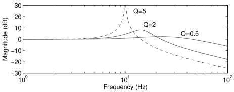
Figure 5: Graph of $|T(j\omega)|$.

The Lagrange multiplier is no longer consistent with ${\lambda}\equiv f_{a}$ in presence of actuator dynamics. Assuming stable contact, one can show from (30) that the constraint force $f_{a}$ is related to the Lagrange multiplier $\lambda$ by

$$f_{a}=T(s)\lambda$$

where

$$T(s) = [I+L(s)]^{-1}L(s)$$ (34)

$$= [{\cal Q}+L^{\prime}(s)I]^{-1}L^{\prime}(s)$$

is the transmissivity transfer function.

Remark 5

Observe that in the presence of actuator dynamics, the force response of the emulating-robot depends on the inertia ratio of the two robots.

A high fidelity emulation requires that $|T(s)|$ be flat over a wide bandwidth and then roll-off at high frequency. The graph of $|T(j\omega)|$ for a scaler case is shown in Fig.5 for $\omega_{p}=10$, $\omega_{a}=25$, and different values of ${\cal Q}$. Note that according to (33), contact stability requires ${\cal Q}<5$. It is evident from the figure that ${\cal Q}$ has to be sufficiently larger than the critical value ${\cal Q}=5$ in order to avoid the resonance.

5 Conclusion

We have presented the development of a methodology for emulation of a target robot, say a space robot, operating in a complex environment by using an actual robot. Although the actual emulating-robot is not dynamically equivalent to the target robot, the former is controlled such that the dynamic similarity is achieved. The emulation scheme aims to replicate the dynamic behavior of the target robot interacting with environment, without dealing with a complex calculation of the contact dynamics. In our approach, the target robot is modelled as a rheonomically constrained manipulator that constitutes a real-time simulator, which together with the control system, drives the actual robot. It has been shown that the Lagrange multipliers corresponding to the constraint is tantamount to a constraint force seen by the simulated robot. Consequently, the difference between the Lagrange multipliers and the physical constraint force is chosen as the force error to be minimized by the controller. To this end, an emulating-robot controller has been developed such that it (i) produces the endpoint motion of the target robot and (ii) regulates the force error to zero.

The fidelity and the stability of the emulation scheme has been analyzed. In this regard, the inertia ratio of the two robots, ${\cal Q}={\cal M}_{s}{\cal M}_{r}^{-1}$, turned out to be an important factor. Specifically, the analysis has yielded the following results:

1. $\|{\cal Q}\|\gg 1$ makes the emulating system sensitive to force/moment sensor noise and disturbance; a low-noise force/moment sensor is required.

2. $\lambda_{max}({\cal Q})\gg 1$ may lead to contact instability due to actuator dynamics and delay; a high bandwidth actuator is required.

3. $\|{\cal Q}\|=1$ minimizes actuation effort; a large deviation from one requires actuators with large torque capacity.

Theses remarks should be considered in design of the emulating robot.

In addition, a number of preliminary experiments for emulation of flexible-joint robots have been performed to support the concept of robot-emulation.

Appendix A

Choose the following Lyapunov function

$$V_{1}=\frac{1}{2}\dot{e}_{p}^{T}\dot{e}_{p}+\frac{1}{2}\dot{e}_{p}^{T}G_{f}{\cal M}_{s}\dot{e}_{p}+\frac{1}{2}e_{p}^{T}G_{p}e_{p},$$

whose time derivative is

$$\dot{V}_{1}=-\frac{1}{2}\dot{e}_{p}^{T}(2G_{v}I-G_{f}\dot{\cal M}_{s})\dot{e}_{p}.$$

Since $\lambda_{i}(2G_{v}I-G_{f}\dot{\cal M}_{s})=2G_{v}-G_{f}\lambda_{i}(\dot{\cal M}_{s})$, we can say $\dot{V}_{1}<0$ if

$$G_{f}<\frac{2G_{v}}{\lambda_{max}(\dot{\cal M}_{s})}.$$

Appendix B

The constraint equations can be linearized up to a first-order approximation by writing the Taylor expansion around a neighborhood, say initial guess $q_{s}^{0}$, as

$$\Phi(q_{s},q_{r})+\Phi_{q_{s}}(q_{s}-q_{s}^{0})\approx 0.$$ (35)

Where the variables $q_{r}$ is considered as a constant value, and $\Phi_{q_{s}}=-J_{s}$. Then, the following loop

$$q_{s}^{k+1}=q_{s}^{k}+J_{s}^{+}{\Phi}(q_{s}^{k},q_{r})$$

can be worked out iteratively until the error in the constraint falls within an acceptable tolerance range, e.g. $\|\Phi\|\leq\epsilon$.

Appendix C

Consider the positive definite function candidate

$$V=\frac{1}{2}\Phi^{T}K\Phi.$$

Its derivative along the trajectories of the system is

$$\dot{V} = \Phi^{T}K\dot{p}_{r}-\Phi^{T}KJ_{s}J_{s}^{T}K\Phi-\Phi^{T}KJ_{s}P\xi$$

$$= \Phi^{T}K\dot{p}_{r}-\Phi^{T}KJ_{s}J_{s}^{T}K\Phi.$$

where the last term in the right-hand side of (C) vanishes because $J_{s}P=0$. An upper bound of $\dot{V}$ is

$$\dot{V}\leq\|\Phi\|\lambda_{M}(K)\|\dot{p}_{r}\|-\|\Phi\|^{2}\lambda_{m}^{2}(K)\lambda_{m}(J_{s}J_{s}^{T}).$$ (37)

Denoting $\lambda_{M}(A)$ and $\lambda_{m}(A)$ as maximum and minimum eigenvalues of matrix $A$, we can find the following condition for negative $\dot{V}$

$$\dot{V}\leq 0,\;\;\;\;\;\forall\|\Phi\|\geq\mu=\frac{\lambda_{M}(K)\|\dot{p}_{r}\|_{max}}{\lambda^{2}_{m}(K)\lambda_{m}(J_{s}J_{s}^{T})}.$$ (38)

Furthermore, we can say the following bounds on the Lyapunov function as

$$\frac{1}{2}\lambda_{m}(K)\|\Phi\|^{2}\leq V\leq\frac{1}{2}\lambda_{M}(K)\|\Phi\|^{2}$$

Therefore, according to the uniform ultimate boundedness theorem of uncertain dynamic system [53, 54], one can say from (37) and (C) that the constraint error $\Phi$ is then uniformly ultimately bounded into the ball centered at $\Phi=0$ and radius

$$\rho=\frac{\gamma^{3/2}(K)\|\dot{p}_{r}\|_{max}}{\lambda_{m}(K)\lambda_{m}(J_{s}J_{s}^{T})},$$

where $\gamma(A)=\lambda_{M}(A)/\lambda_{m}(A)$ is the condition number of matrix A, which concludes the proof. Note that $K$ can be conveniently chosen as a diagonal matrix $K=kI$, and hence $\gamma=1$ and $\lambda_{m}(K)=k$. Then, the error can be diminished at will by increasing $k$ [37].

Appendix D

The Routh-Hurwitz schedule of the coefficients of the characteristic equation is

$$\begin{array}[]{rl}{\begin{array}[]{l}s^{3}\\ s^{2}\\ s\\ 1\end{array}}&{\left|\begin{array}[]{ll}\lambda_{i}({\cal Q})/\epsilon\omega_{a}&G_{v}\\ 1&G_{p}\\ G_{v}-\lambda_{i}({\cal Q})G_{p}/\epsilon\omega_{a}&0\\ G_{p}&0\end{array}\right.}\end{array}$$

The Routh-Hurwitz criterion states that the number of roots of the characteristic equation with positive real parts is equal to the number of changes in the sign of the first column array.

Appendix E

In this appendix, the control algorithm for emulation of 1-dof flexible joint arm is developed. The dynamics of a 1-dof flexible joint arm can be expressed by [49, 50]

$$\!\!\left[\begin{array}[]{c}m_{s1}\ddot{q}_{s1}\\ m_{s2}\ddot{q}_{s2}\end{array}\right]\!\!=\!\!\left[\begin{array}[]{c}k(q_{s2}-q_{s1})+\zeta(\dot{q}_{s2}-\dot{q}_{s1})\\ -k(q_{s2}-q_{s1})-\zeta(\dot{q}_{s2}-\dot{q}_{s1})-c_{s}\dot{q}_{s2}+\tau_{s}(t)\end{array}\right]$$

where $m_{s1}=0.05kgm^{2}$ and $m_{s2}=0.1kgm^{2}$ are the link inertia and the drive inertia, $l=0.3m$ is the arm length, $k=3.0Nm/rad$ represents joint stiffness, $\zeta=0.1Nm.s/rad$ is damping at joint, and $\tau_{s}(t)$ is real-time control input of the simulated robot – in this particular illustration, the control law is comprised of the resolved-rate controller accompanied with a force-moment accommodation (FMA) loop [55].

The dynamics of the rigid joint robot is simply described by

$$m_{r}\ddot{q}_{r}+c_{r}\dot{q}_{r}+w\cos(q_{r})=\tau_{r}+fl$$

where $c_{r}=0.022Nm.s/rad$ represents joint viscous friction, and $m_{r}=0.05kgm^{2}$ is the collective arm inertia, and $w=0.5Nm$ is the maximum gravity torque. Since $J_{s1}=J_{r}=l$, we have $q_{s1}\equiv q_{r}$. Hence, the control law for the rigid robot makes it behave as a flexible joint robot whose dynamics is expressed by

$$\tau_{r} = c_{r}\dot{q}_{r}+w\cos(q_{r})-fl+m_{r}m_{s1}^{-1}[\ddot{q}_{s1}$$

$$+ G_{v}(\dot{q}_{r}-\dot{q}_{s1})+G_{p}(q_{r}-q_{s1})],$$

where

$$\dot{\xi}=m_{s2}^{-1}[-k(\xi-q_{r})-\zeta(\dot{\xi}-\dot{q}_{r})+\tau_{s}(t)],$$

and

$$\ddot{q}_{s1}=m_{s1}^{-1}[k(\xi-q_{r})+\zeta(\dot{\xi}-\dot{q}_{r})].$$

References

- [1] F. Aghili and J.-C. Piedboeuf, “Emulation of robots interacting with environment,” IEEE/ASME Trans. on Mechatronics, vol. 11, no. 1, pp. 35–46, Feb. 2006.
- [2] S. B. Skaar, C. F. Rouff, and A. R. Seebass, Teleoperation and Robotics in Space. Washington, DC: American Institute of Aeronautics and Astronautics, Inc., 1994.
- [3] F. Aghili, “Cartesian control of space manipulators for on-orbit servicing,” in AIAA Guidance, Navigation and Control Conference, Toronto, Canada, August 2010.
- [4] F. Aghili and C.-Y. Su, “Reconfigurable space manipulators for in-orbit servicing and space exploration,” in International Symposium on Artificial Intelligence, Robotics and Automation in Space i-SAIRAS, Turin, Italy, Sep. 4–6 2012.
- [5] F. Aghili, “Active orbital debris removal using space robotics,” in International Symposium on Artificial Intelligence, Robotics and Automation in Space i-SAIRAS, Turin, Italy, Sep. 4–6 2012.
- [6] J.-C. Piedbœuf, F. Aghili, M. Doyon, and E. Martin, “Dynamic emulation of space robot in one-g environment using hardware-in-loop simulation,” in CISM-IFToMM Symposium on Robotics Design, Dynamics and Control, Italy, July 3–6 2002.
- [7] F. Aghili and J.-C. Piedbœuf, “Contact dynamics emulation for hardware-in-loop simulation of robots interacting with environment,” in IEEE International Conference on Robotics & Automation, Washington, USA, May 11–15 2002, pp. 534–529.
- [8] F. Aghili, “A prediction and motion-planning scheme for visually guided robotic capturing of free-floating tumbling objects with uncertain dynamics,” IEEE Transactions on Robotics, vol. 28, no. 3, pp. 634–649, June 2012.
- [9] F. Aghili and A. Salerno, Multisensor Attitude Estimation and Applications, 1st ed. CRC Press, 2016, ch. Adaptive Data Fusion of Multiple Sensors for Vehicle Pose Estimation.
- [10] F. Aghili and K. Parsa, “Adaptive motion estimation of a tumbling satellite using laser-vision data with unknown noise characteristics,” in 2007 IEEE/RSJ International Conference on Intelligent Robots and Systems, Oct 2007, pp. 839–846.
- [11] J.-C. Piedbœuf, E. Dupuis, and J. de Carufel, “STVF concept document,” Canadian Space Agency, St-Hubert, Quebec, Tech. Rep. CSA-SS-ST-016, Feb. 1998.
- [12] F. Aghili, E. Dupuis, J.-C. Piedbœuf, and J. de Carufel, “Hardware-in-the-loop simulations of robots performing contact tasks,” in International Symposium on Artificial Intelligence and Robotics & Automation in Space: i-SAIRAS, M. Perry, Ed. Noordwijk, The Netherland: ESA Publication Division, 1999, pp. 583–588.
- [13] F. Aghili, “Robust impedance-matching of manipulators interacting with uncertain environments: Application to task verification of the space station’s dexterous manipulator,” IEEE/ASME Transactions on Mechatronics, vol. 24, no. 4, pp. 1565–1576, Aug 2019.
- [14] J.-C. Piedbœuf, F. Aghili, M. Doyon, Y. Gonthier, E. Martin, and W.-H. Zhu, “Emulation of space robot through hardware-in-the-loop simulation,” in The 6th International Symposium on Artificial Intelligence and Robotics & Automation in Space: i-SAIRAS, Canadian Space Agency, St-Hubert, Quebec, Canada, Jun. 18–22 2001.
- [15] J.-C. Piedbœuf, J. de Carufel, F. Aghili, and E. Dupuis, “Task verification facility for the Canadian special purpose dextrous manipulator,” in IEEE Int. Conf. on Robotics & Automation, Detroit, Michigan, May 10–15 1999, pp. 1077–1083.
- [16] J. de Carufel, E. Martin, and J.-C. Piedbœuf, “Control strategies for hardware-in-the-loop simulation of flexible space robots,” IEEE Proceedings-D: Control Theory and Applications, vol. 147, no. 6, pp. 569–579, 2000.
- [17] O. Ma, K. Buhariwala, N. Roger, J. MacLean, and R. Carr, “MDSF- A generic development and simulation facility for flexible, complex robotic systems,” vol. 15, pp. 49–62, 1997.
- [18] Z. Vafa and S. Dubowsky, “The kinematics and dynamics of space manipulators: The virtual manipulator approach,” vol. 9, no. 4, pp. 3–21, Aug. 1990.
- [19] ——, “On the dynamics of space manipulators using the virtual manipulator, with applications to path planning,” vol. 38, no. 4, pp. 441–472, Oct.–Dec. 1990.
- [20] O. Ma and M. Nahon, “A general method for computing the distance between two moving objects using optimization techniques,” ASME Advances in Design Automation, vol. 1, pp. 109–117, 1992, dE-Vol.44-1.
- [21] H. M. Lankarani and P. E. Nikravesh, “Application of the canonical equations of motion in problems of constrained multibody systems with intermittent motion,” in ASME Design Automation Conference. Orland (Florida): ASME, 1988, aSME-Paper No. 88-DAC-51.
- [22] K. L. Johnson, Contact Mechanics. London: Cambridge University Press, 1985.
- [23] S. Dubowsky, W. Durfee, A. Kulinski, U. Müller, I. Paul, and J. Pennington, “The design and implementation of a laboratory test bed for space robotics: The ves mod II,” in ASME Conf. DE-Vol. 72, Robotics: Kinematics, Dynamics and Control, 1994, pp. 99–108.
- [24] R. Krenn and B. Schäfer, “Limitations of hardware-in-the-loop simulations of space robotics dynamics using industrial robots,” M. Perry, Ed. Noordwijk, The Netherland: ESA Publication Division, 1999, pp. 681–686.
- [25] S. Ananthakrishnan, R. Teders, and K. Alder, “Role of estimation in real-time contact dynamics enhancement of space station engineering facility,” IEEE Robotics & Automation Magazine, no. 3, pp. 20–28, Sep. 1996.
- [26] F. Aghili, “A mechatronics testbed for manipulator joints,” in IEEE Int. Conference on Robotics & Automation, Orlando, Florida, May 2006, pp. 2188–2194.
- [27] S. Tarao, E. Inohira, and M. Uchiyama, “Motion simulation using a high-speed parallel link mechanism,” in The 2000 IEEE/RSJ Int. Conf. On Intelligent Robots and Systems, Takamatsu, Japan, 2000.
- [28] F. Aghili and M. Namvar, “Scaling inertia properties of a manipulator payload for 0-g emulation of spacecraft,” The International Journal of Robotics Research, vol. 28, no. 7, pp. 883–894, July 2009.
- [29] F. Aghili, “A robotic testbed for zero-g emulation of spacecraft,” in IEEE/RSJ Int. Conference on Intelligent Robots and Systems, Edmonton, Alberta, Canada, 2005, pp. 1033–1040.
- [30] F. Aghili, M. Namvar, and G. Vukovich, “Satellite simulator with a hydraulic manipulator,” in IEEE Int. Conference on Robotics & Automation, Orlando, Florida, May 2006, pp. 3886–3892.
- [31] F. Aghili and K. Parsa, “Motion and parameter estimation of space objects using laser-vision data,” AIAA Journal of Guidance, Control, and Dynamics, vol. 32, no. 2, pp. 538–550, March 2009.
- [32] F. Aghili, “A mechatronic testbed for revolute-joint prototypes of a manipulator,” IEEE Trans. on Robotics, vol. 22, no. 6, pp. 1265–1273, Dec. 2006.
- [33] F. Aghili, K. Parsa, and E. Martin, “Robotic docking of a free-falling space object with occluded visual condition,” in 9th Int. Symp. on Artificial Intelligence, Robotics & Automation in Space, Los Angeles, CA, Feb. 26 – 29 2008.
- [34] F. Aghili and C. Y. Su, “Robust relative navigation by integration of icp and adaptive kalman filter using laser scanner and imu,” IEEE/ASME Transactions on Mechatronics, vol. 21, no. 4, pp. 2015–2026, Aug 2016.
- [35] F. Aghili, “Optimal control for robotic capturing and passivation of a tumbling satellite with unknown dyanmcis,” in AIAA Guidance, Navigation and Control Conference, Honolulu, Hawaii, August 2008.
- [36] ——, “Automated rendezvous & docking (AR&D) without impact using a reliable 3d vision system,” in AIAA Guidance, Navigation and Control Conference, Toronto, Canada, August 2010.
- [37] C. Canudas de Wit, B. Siciliano, and G. Bastin, Eds., Theory of Robot Control. London, Great Britain: Springer, 1996.
- [38] J. J. Craig, Introduction to Robotics: Mechanical and Control, 2nd ed. Reading, Massachusetts: Addison-Wesley Publishing Company, 1989.
- [39] J. G. de Jalon and E. Bayo, Kinematic and Dynamic Simulation of Multibody Systems. Springer-Verlag, 1989.
- [40] F. Aghili, “A unified approach for inverse and direct dynamics of constrained multibody systems based on linear projection operator: Applications to control and simulation,” IEEE Trans. on Robotics, vol. 21, no. 5, pp. 834–849, Oct. 2005.
- [41] F. Aghili and J.-C. Piedbœuf, “Simulation of motion of constrained multibody systems based on projection operator,” Journal of Multibody System Dynamics, vol. 10, pp. 3–16, 2003.
- [42] F. Aghili and K. Parsa, “An adaptive vision system for guidance of a robotic manipulator to capture a tumbling satellite with unknown dynamics,” in IEEE/RSJ Int. Conf. on Intelligent Robots and Systems, Nice, France, September 2008, pp. 3064–3071.
- [43] M. W. Spong and M. Vidyasagar, Robot Dynamics and Control. New York, NY: Wiley, 1989.
- [44] F. Aghili, “Robust impedance control of manipulators carrying heavy payload,” ASME Journal of Dynamic Systems, Measurements, and Control, vol. 132, September 2010.
- [45] W. A. Wolovich and H. Elliott, “A computational technique for inverse kinematics,” in IEEE Conf. On Decision and Control, New York, 1984, pp. 1359–1363.
- [46] P. Chiacchio, S. Chiaverini, L. Sciavicco, and B. Siciliano, “Closed-loop inverse kinematics schemes for constrained redundant manipulators with task space augmentation and task priority strategy,” The Int. Journal of Robotics Research, vol. 10, no. 4, pp. 410–425, Aug. 1991.
- [47] A. Balestrino, G. D. Maria, and L. Sciavicco, “Robust control of robotic manipulators,” Reprint of the 9th IFAC World Congress, vol. 6, pp. 80–85, Jul. 1984.
- [48] J. Garcia de Jalón and E. Bayo, Kinematic and Dynamic Simulation of Multibody Systems: The Real-Time Challenge. New York: Springer-Verlag, 1994.
- [49] P. Tomei, “A simple PD controller for robots with elastic joints,” IEEE Trans. on Automatic Control, vol. 36, pp. 1208–1213, 1991.
- [50] K. P. Jankowski and H. A. ElMaraghy, “Dynamic control of flexible joint robots with constrained end-effector motion,” in Prepr. 3rd IFAC Symp. On Robot Control, Vienna, 1991, pp. 345–350.
- [51] S. Skogestad and I. Postlethwaite, Multivariable Feedback Control Analysis and Design. West Sussex PO19 1UD, England: John Wiley & Sons, 1996.
- [52] W. R. Evans, “Control system synthesis by root locus method,” Transactions of the AIEE, vol. 69, pp. 1–4, 1954.
- [53] M. J. Corless and G. Letmann, “Continous state feedback guaranteeing uniform ultimate boundedness for uncertain dynmamic systems,” IEEE Trans. on Automatic Control, vol. AC-26, no. 5, pp. 1139–1144, Oct. 1981.
- [54] H. K. Khalil, Nonlinear Systems. New-York: Macmillan Publishing Company, 1992.
- [55] F. Aghili, E. Dupuis, E. Martin, and J.-C. Piedbœuf, “Force/Moment accommodation control for tele-operated manipulators performing contact tasks in stiff environment,” in Proceedings of the 2001 IEEE/RSJ International Conference on Intelligent Robotics and Systems, Maui, Hawaii, USA, Oct. 29–Nov. 03 2001, pp. 2227 – 2233.