Time-resolved Coulomb collision of single electrons

Abstract

Precise control over interactions between ballistic electrons will enable us to exploit Coulomb interactions in novel ways, to develop high-speed sensing,¹ to reach a non-linear regime in electron quantum optics and to realise schemes for fundamental two-qubit operations² on flying electrons. Time-resolved collisions between electrons have been used to probe the indistinguishability,³ Wigner function^{4, 5} and decoherence⁶ of single electron wavepackets. Due to the effects of screening, none of these experiments were performed in a regime where Coulomb interactions were particularly strong. Here we explore the Coulomb collision of two high energy electrons in counter-propagating ballistic edge states.^{7, 8} We show that, in this kind of unscreened device, the partitioning probabilities at different electron arrival times and barrier height are shaped by Coulomb repulsion between the electrons. This prevents the wavepacket overlap required for the manifestation of fermionic exchange statistics but suggests a new class of devices for studying and manipulating interactions of ballistic single electrons.

In principle, time-resolved electronic interactions can be studied with a wavepacket collider like that sketched in Fig. 1. Single electron sources S1 and S2 emit particles with relative delay $t_{\rm 21}$ into an experimentally-defined collision region. Interactions determine how particles are partitioned into detectors D1 and D2 for different injection time.^{3, 9} Under some conditions, fermionic exchange effects can create antibunching of wavepackets, detected via reduced current noise at the detectors.³ This effect can be used as a measurement of the indistinguishability of the wavepackets, an important figure of merit for quantum coherent transport.¹⁰ However, in general, understanding the behaviour of the electrons in the interaction region is not straightforward if direct Coulomb effects are present in addition to exchange effects.¹¹

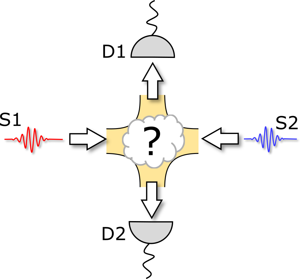
Figure 1: Idealised electronic wavepacket collider Sources S1, S2 inject electrons into a collision region with a variable time delay. They interact and scatter into detectors D1 and D2. This can be used to study interactions between electrons, interactions with the environment, and behaviour of the electron sources.

For sources injecting electrons near the Fermi energy, the impact of the Coulomb interaction on the electron trajectory is diminished by screening.³ Changes to the single electron trajectories or velocity from direct Coulomb interactions between single electrons has not been seen, although coupling to nearby conducting channels has been detected via decoherence of the wavepackets.⁶ Where electronic density is reduced, or for particles injected at higher energy, the trajectories and velocity of electrons are expected to be significantly modified.^{12, 13} Understanding this regime is important for the controlled use of Coulomb interactions for quantum logic gates.¹⁴

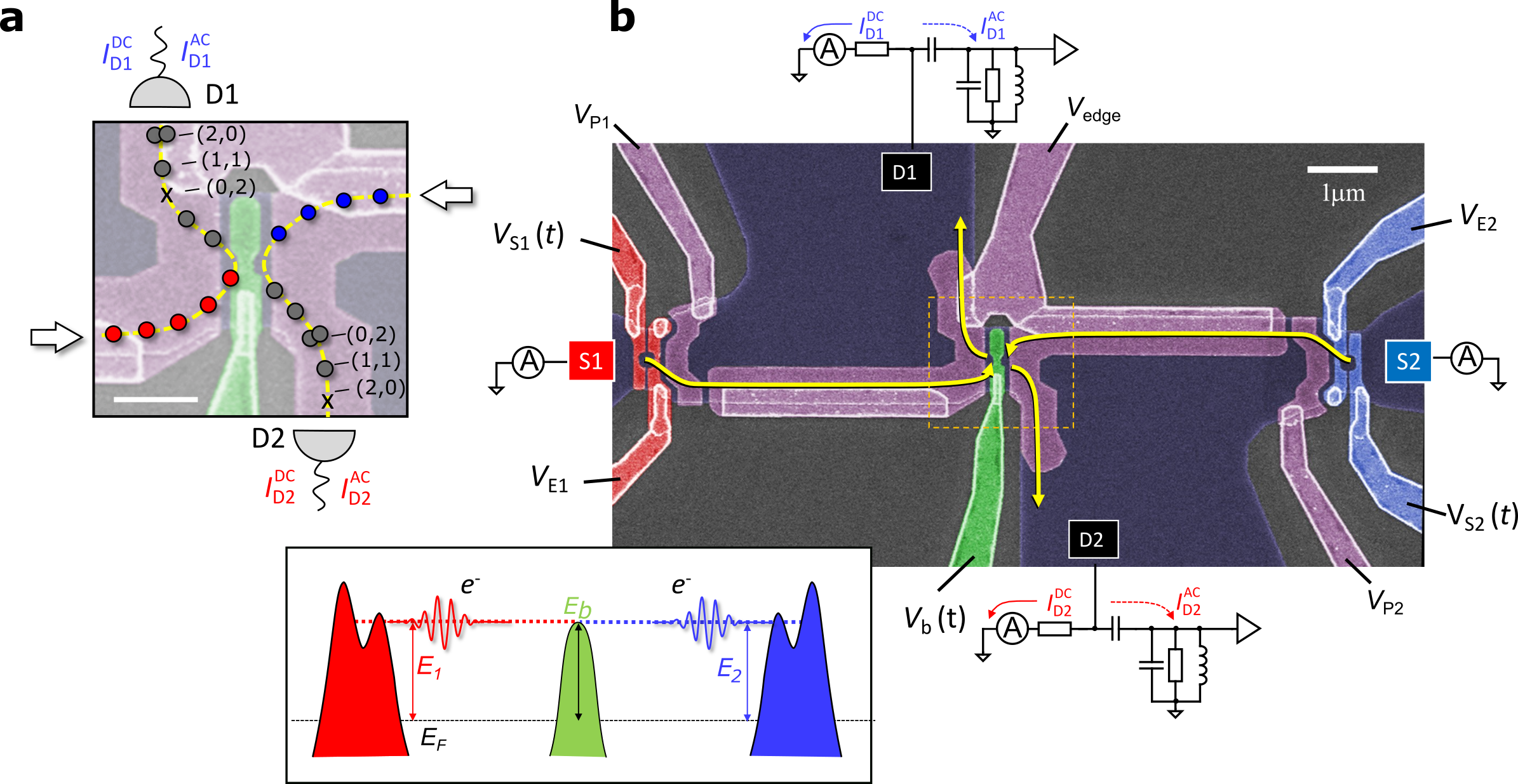
Figure 2: Electron collider implemented with high energy single electrons (a) Partitioning of electrons in a high energy device. Three outcomes are characterised by charge distributions (2,0) when both electrons enter D1, (0,2) when both enter D2, and (1,1) one enters each. Scalebar length is 500 nm. Proximity of electrons is exaggerated for clarity (see methods for timing information). (b) False colour scanning electron microscopy image of overall device structure and measurement system. See methods for details. Electrons emitted from sources S1 (left, red) and S2 (right, blue) eject electrons follow trajectories indicated by arrows, colliding at the central barrier (green). Dashed region indicates the collision region shown in (a). Inset: Energy level drawing to show adjustable ejection energy.

To learn how to harness the Coulomb repulsion in ballistic electron systems, we have studied an electron collider based on electron pumps which emit electrons into edge states at high energy ($E>100$ meV).^{7, 8, 15, 16} In this case, the time-resolved Coulomb interaction between ballistic single electrons can be directly detected.

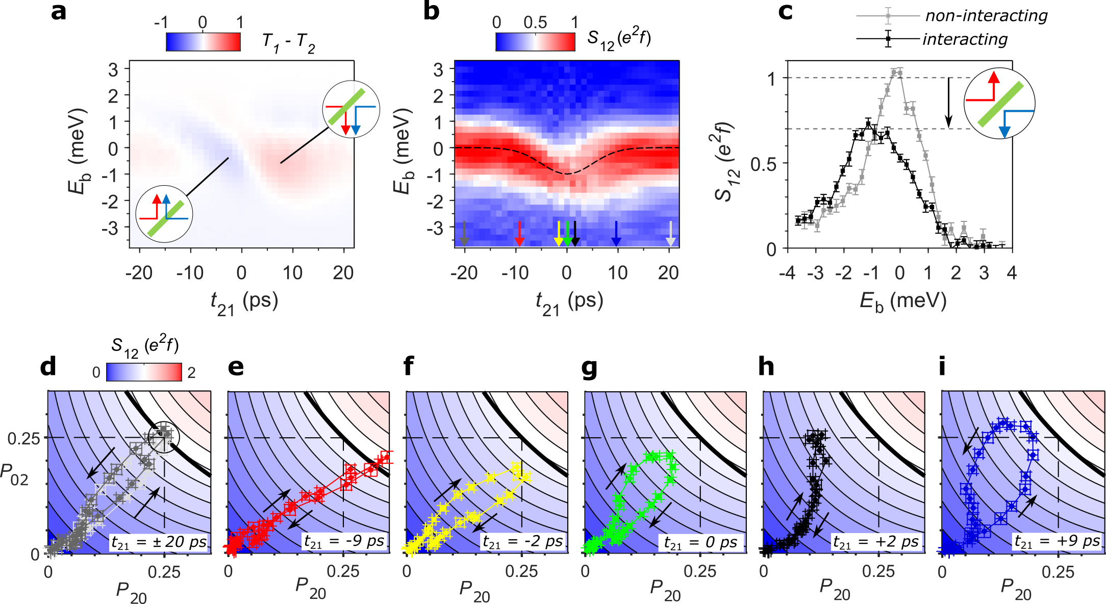
Figure 3: Current imbalance, shot noise suppression and partition statistics (a) Current imbalance $T_{1}-T_{2}$ for different barrier height $E_{\rm b}$ and time delay $t_{\rm 21}$. Favoured events associated with the negative and positive current imbalances are indicated schematically. (b) Map of shot noise $S_{12}$ for barrier height $E_{\rm b}$ and time delay $t_{\rm 21}$. Dashed line is a guide to peak noise position. (c) Shot noise $S_{12}$ in the non-interacting ($t_{\rm 21}=-20$ ps) and strongly interacting regime ($t_{\rm 21}=+2$ ps) where the effect is most pronounced. Reduction in noise is associated with repulsion events as indicated. For estimation of errors bars, see Supplementary Section 1. Each panel (d-i) shows partition probabilities ($P_{20}$, $P_{02}$) at different barrier heights for a chosen $t_{21}$. Underlying colour map shows noise $S_{12}$ (contour lines are at $0.1e^{2}f$ intervals). (d) The non-interacting case (electrons miss each other) at $t_{\rm 21}=-20$ ps (dark grey) +$20$ ps (light grey). Arrows show the sweep from high to low barrier height, reaching the maximum noise at independent scattering limit (thick solid line). At this point $(P_{20},P_{02})=(0.25,0.25)$ (circled) there are an equal statistical mixture of each outcome event. (e-i) as (d) but for selected interacting cases $t_{\rm 21}=-9,-2,0,+2,+9$ ps corresponding to arrows in panel b. These cases show a strongly modified behaviour as described in the text.

The collision region of the electron collider is shown in Fig. 2a and the overall device structure in Fig. 2b. Electron pump sources S1 (left) and S2 (right) each inject an electron every $\tau=2$ ns.¹⁷ In a perpendicular magnetic field these are confined to states on the mesa-edge with energies $E_{1}$ and $E_{2}$ typically in excess of 100 meV.⁷ These can be individually tuned⁷ such that $E_{1}\simeq E_{2}$. Trajectories meet at a barrier with height $E_{\rm b}$ set by a gate voltage (see methods). At the barrier, electrons from source 1 and 2 are transmitted with probabilities $T_{1}$ and $T_{2}$ into output arms D2 and D1, respectively. The emission times from the two sources can be fine-tuned so that the nominal difference between arrival times at the centre barrier $t_{\rm 21}=t_{2}-t_{1}$ can be chosen arbitrarily. For $t_{\rm 21}=0$ arrival is synchronised (see methods), down to a residual uncertainty determined by the emission time variation of the sources, typically of order picoseconds.¹⁶

When only one source is active, individual $T_{n}(E_{\rm b})$ can be measured from the time-averaged current.^{7, 16} For our two sources we find that $T_{1}(E_{\rm b})\simeq T_{2}(E_{\rm b})$. When both sources are active, the current at detector D2 is $I_{\rm D2}^{\rm DC}=ef(T_{1}+1-T_{2})$ i.e. collecting any electrons from source S1 transmitted through the barrier and those from source S2 reflected by the barrier. Similarly $I_{\rm D1}^{\rm DC}=ef(T_{2}+1-T_{1})$.

For deliberately mismatched arrival times $I_{\rm D1}^{\rm DC}=I_{\rm D2}^{\rm DC}\simeq ef$, a nearly constant background. When arrival times are synchronised to within a few picoseconds (Supplementary Section 1) an imbalance in transmission is seen. We show this, calculated using $T_{1}-T_{2}=(I_{\rm D2}^{\rm DC}-I_{\rm D1}^{\rm DC})/2ef$, in Fig. 3a. For values near $t_{\rm 21}=0$ we see a pronounced current imbalance with $T_{1}-T_{2}\simeq+0.2$ for $t_{\rm 21}>0$ and $T_{1}-T_{2}\simeq-0.2$ for $t_{\rm 21}<0$. The polarity of this signal corresponds to preferential transmission of the earlier electron.

Measuring the time-dependent noise current, $I_{\rm D1}^{\rm AC},I_{\rm D2}^{\rm AC}$ using the additional connections shown in Fig. 2b enables us to measure correlations^{3, 8} in partitioning outcomes from individual scattering cycles that are not accessible in a time-averaged measurement. The shot noise current $S_{12}$, simultaneously measured in contacts D1 and D2 (see methods), is mapped as a function of $E_{\rm b}$ and $t_{\rm 21}$ in Fig. 3b. In the case $|t_{\rm 21}|\gg 0$, electrons arrive at very different times and do not interact. The noise signal in this regime is explained by independent stochastic transmission of the electrons into either D1 or D2 given by $S_{12}=2e^{2}f\sum_{n=1,2}[T_{n}(1-T_{n})]$.⁸ The noise $S_{12}\simeq 0$ when the barrier is much higher or lower than the injection energy, but reaches a peak $S_{12}|_{\rm max}=e^{2}f$ when $E_{\rm b}\simeq E_{1}\simeq E_{2}$ and $T_{1},T_{2}\simeq 0.5$ (i.e. the noise peak can pick out the electron energy).

The noise is modified in several ways by Coulomb interactions. Firstly, for values of $t_{\rm 21}\simeq 0$ (i.e. electrons collide), the position of the noise peak moves to a lower value of the programmed barrier height $E_{\rm b}$. This apparent shift in detected energy, $E_{1}\rightarrow E_{1}^{\prime}$ and $E_{2}\rightarrow E_{2}^{\prime}$ is a manifestation of the Coulomb repulsion between the electrons which gives a transient increase in the effective barrier height of $\simeq 0.5-1$ meV. Conservation of energy is preserved by a reduction in the kinetic energy corresponding to the increased Coulomb repulsion.¹³ Secondly, at delay times near $t_{\rm 21}=0$ the maximum partition noise $S_{12}|_{\rm max}$ is reduced from the independent scattering limit by up to $\simeq 30$%, as shown in Fig.3(c). This effect is driven by an increase in the number of events where both electrons are reflected due to a repulsive interaction. While the noise reduction is in superficial resemblance to a partial Pauli dip,³ we show below that the full partitioning statistics, calculated from the time-averaged current and noise data,⁸ reveal a Coulomb-dominated system.

The partition probabilities for the three possible detector charge states $P_{ij}$ are $P_{20},P_{11},P_{02}$ where $i,j$ are the number of electrons in detector D1, D2 and $\sum P_{ij}=1$. Particular values of $P_{02},P_{20}$ map directly to current noise and time-averaged current distribution.^{8, 18} Computed values of $P_{02},P_{20}$ at different barrier height are shown in Fig. 3d-i. The non-interacting case in Fig. 3d ($|t_{\rm 21}|=20$ ps) has $P_{02},P_{20}\simeq 0,P_{11}\simeq 1$ for high and low barriers and the expected statistical mixture of outcomes when $E_{\rm b}\simeq E_{1},E_{2}$ namely $P_{02}|_{\rm max},P_{20}|_{\rm max}\simeq 0.25$ and $P_{11}|_{\rm min}\simeq 0.5$. The results in the interacting regime ($|t_{\rm 21}|<10$ ps) are shown in Fig. 3e-i. Preferential transmission into D1 or D2 causes an imbalance in $P_{20}$ and $P_{02}$ (a tilt toward the $P_{02}$ or $P_{20}$ axis). $P_{20}|_{\rm max}$ and $P_{02}|_{\rm max}$ are also suppressed below the independent scattering value $\sqrt{P_{20}}+\sqrt{P_{02}}=1$ (thick solid line in Fig. 3d-i). This corresponds to a reduction in noise or an excess antibunching $\Delta P_{11}=P_{11}|_{\rm min}-0.5\simeq 0.15$.

We show below that the full partitioning dataset is fully captured by a model of the microscopic trajectories which follow the $E\times B$ drift motion. The shape of these trajectories is set by the partitioning barrier potential and the (weakly screened) Coulomb interaction. We also show that the small timing and energy fluctuations of the source¹⁶ are important in determining the statistical outcomes seen experimentally.

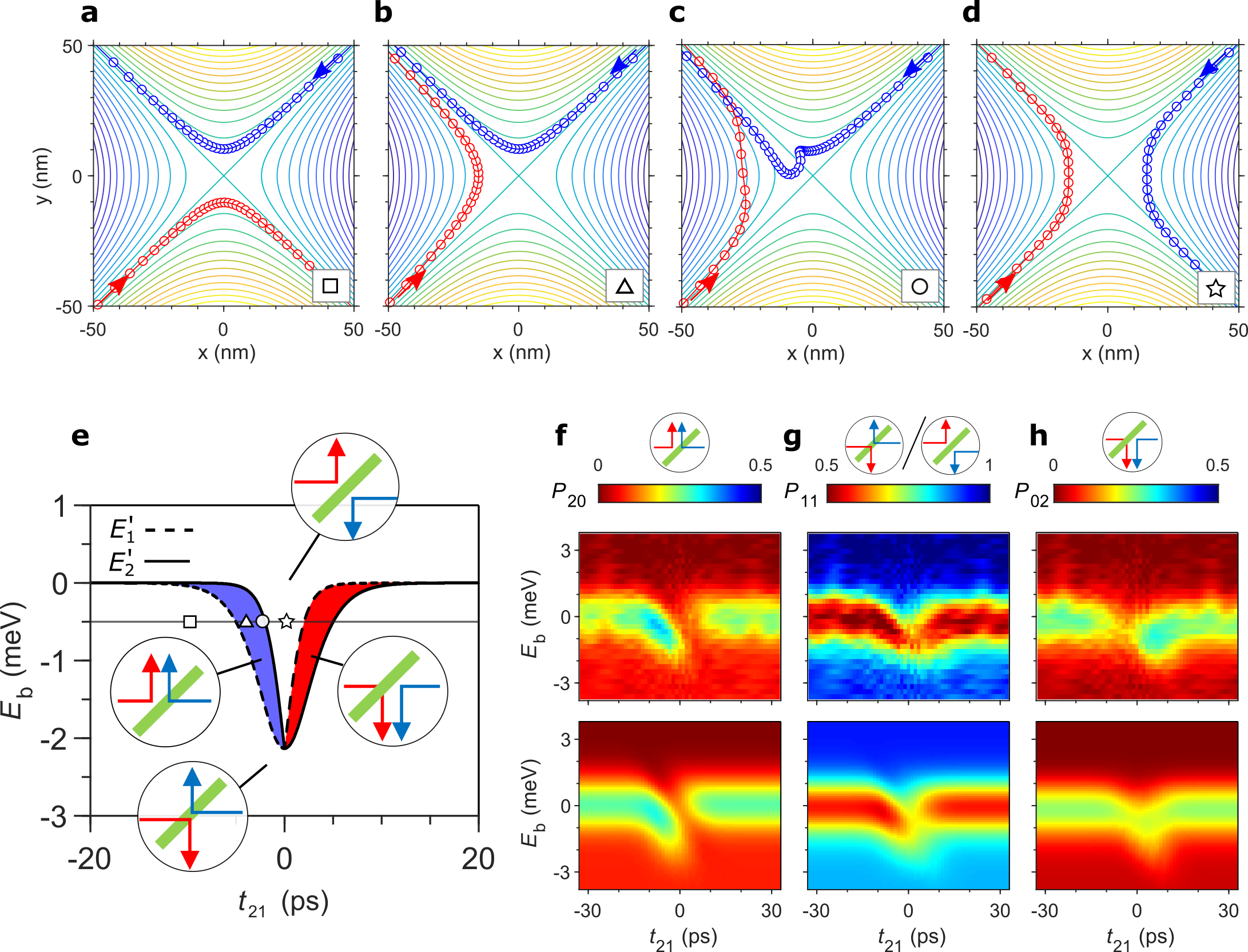
Figure 4: Trajectory of interacting electrons and the resulting partition statistics: (a-d) Electron trajectories for electrons colliding near the saddle point barrier at $E_{1}=E_{2}=E_{\rm b}+0.5$ meV. (a) $t_{\rm 21}=-10$ ps non-interacting case; the electron from source S2 arrives first. Electrons from source S1 and S2 are both transmitted. (b) $t_{\rm 21}=-4$ ps; S2 electron arrives first and is transmitted, but blocks S1 electron. (c) $t_{\rm 21}=-2.5$ ps; same outcome as (b), but exit of the S2 electron from the scattering region is delayed. (d) $t_{\rm 21}=0$ ps; electrons block each other at the barrier and both are reflected. By symmetry, corresponding trajectories are found for $t_{\rm 21}>0$ (not shown). (e) Transmission imbalance $T_{1}-T_{2}=-1,0,1$ (blue, white, red) as a function of $t_{\rm 21}$ and $E_{\rm b}$ for $E_{1}\simeq E_{2}$. Four regions of uniform $T_{1}-T_{2}$ are seen. Two have uneven transmission distribution (areas shaded red and blue) while two have an even charge distribution (shaded white) which correspond to cases where electrons are are both reflected or both transmitted. Dotted ($E_{1}^{\prime}$) and solid ($E_{2}^{\prime}$) lines mark individual transmission thresholds for electrons from source S1 and S2. Symbols ($\square,\triangle,\medcircle,\medstar$) indicate the specific values of $(t_{\rm 21},E_{\rm b})$ used for the trajectories in panels a-d. (f), (g), (h) upper panels show full maps of experimentally obtained probabilities $P_{20}$, $P_{11}$, $P_{02}$. Lower panels show calculation of ensemble average over classical outcomes

We compute the trajectories for an assumed form of the potential¹⁹ near the barrier $U_{\rm 2D}(x,y)$ and an interaction potential $U_{ee}(\vec{r_{1}},\vec{r_{2}})\propto 1/r$ at short range, but which weakens at longer distances ($r_{12}\gg 90$ nm, see methods) due to screening by metallic surface gates.²⁰ Interactions are limited to a region within the screening length near the effective tunneling point, making a saddle point barrier potential an appropriate approximation.¹⁹ Calculations based on the $E\times B$ trajectories are valid in the regime of our experiments where the energy window of quantum scattering (over which the barrier transmission probability changes from 0 to 1) is much smaller than the energy uncertainty of the electrons and/or the purity of the electrons is sufficiently low ¹⁶ (see Supplementary Section 2).

Example trajectories are shown in Fig. 4 for injection energy exceeding the barrier height $E_{n}-E_{\rm b}=0.5$ meV. This illustrates three important cases; completely mismatched arrival Fig. 4a, near-synchronised Fig. 4b,c and closely synchronised Fig. 4d. In the non-interacting case Fig. 4a, trajectories follow the equipotential contours of $U_{2D}$ and the transmitted charge $(Q_{T1},Q_{T2})=(1e,1e)$. In contrast, close to synchronisation as in Fig. 4d, both electrons are deflected such that $(Q_{T1},Q_{T2})=(0e,0e)$. For the near-synchronised cases in Fig. 4b,c interactions modify the trajectory of the electrons in a more complicated way. The late-arriving electron (from S1 in these examples) tends to be deflected by the earlier-arriving electron (here from S2) which blocks the barrier region. This leads to $(Q_{T1},Q_{T2})=(0e,1e)$ for a range of $t_{\rm 21}$ including examples like those shown in Fig. 4b and c.

Establishing that the order-of-arrival effect described above is accessible experimentally would show that the Coulomb interaction can be controlled on the time-scales relevant for interactions in edge states. We numerically compute a large number of trajectories at different injection energies $E_{1}-E_{b},E_{2}-E_{b}$ and relative arrival time $t_{21}$, making a detailed map of the charge partitioning outcomes (see Supplementary Section 2). We use this to reveal how details of the Coulomb interaction appear in experimental partitioning data.

The transmission imbalance $T_{1}-T_{2}$ is plotted in Fig. 4e, computed from the charge distribution $(Q_{T1},Q_{T2})$ at various arrival time delays and barrier heights for equal injection energy $E_{1}=E_{2}$. This map consists of four regions, encompassing the specific example trajectories in Fig. 4a-d (see markers). Each region is bounded by the values of $E_{\rm b}=E_{n}^{\prime}$, the programmed barrier height at which the first or second electrons stop being transmitted in the presence of Coulomb repulsion. The functional form of $E_{n}^{\prime}(t_{\rm 21})$ is an asymmetric peak created by the accumulated effect of the Coulomb interaction during the interaction. In the region where the peaks overlap, there is a regime where the electrons repel, as in Fig.4(d). At larger values of $|t_{\rm 21}|$, when electron arrival is not exactly synchronised, the asymmetry gives $E_{1}^{\prime}(t_{\rm 21})\neq E_{2}^{\prime}(t_{\rm 21})$. This is because generally the effective kinetic energy loss of each particle is different. This creates an intermediate region where only the late-arriving electron is blocked. This predicts a current imbalance in $T_{1}-T_{2}=-1,0,+1$ with the same polarity as that measured experimentally in Fig. 3a. This suggests that the fine structure in the time-resolved Coulomb collision described above is indeed visible experimentally, but appears broadened.

In this calculation, we find that the exact values of $E_{n}^{\prime}$ and the range of $t_{\rm 21}$ over which the interaction extends $t_{\omega}$ are governed by the cyclotron frequency, the curvature of the saddle point $\omega_{xy}=\sqrt{\omega_{x}\omega_{y}}$ and the inclusion of screening. However, the qualitative behaviour of the partitioning map is not sensitive to the precise parameters used. A more important consideration for comparison with experiment is that the map of outcomes in Fig. 4e captures classical behaviour for well-defined injection energies and times. A finite phase-space area for electronic injection energy and time is expected²¹ along with extrinsic emission time and energy fluctuations of the source.¹⁶ These effects will broaden the boundaries of the different scattering outcomes as the barrier height and time of arrival vary. This has an impact on the maximum visibility of the order-of-arrival effects, completely smearing them out in the case of grossly time-broadened emission (see Supplementary Section 1).

We compute the partition probabilities $P_{20},P_{11},P_{02}$ from the ensemble average of the charge distribution $(Q_{T1},Q_{T2})$ over the initial conditions $(E_{1},E_{2},t_{21})$ of the trajectories obtained from the source energy-time distribution (i.e. energy, time widths $\sigma_{t}$ and $\sigma_{E}$ measured for each source, see methods).

The full experimental partition statistics and the computed ensemble average are shown together in Fig 4f-h. The agreement between the experimental data (upper panels) and model calculations (lower panels) show that the Coulomb interaction, broadened by the fluctuations of the electrons sources, is accessible experimentally. Overall, the ensemble effects blurs the sharp boundaries of the classical outcomes, reducing the size of the shift in the noise peak. The energy-time correlation present in the emission distributions, a characteristic feature of the source,¹⁶ and mismatches between the exact source emission distributions explains the fine structure of the partitioning data. That the energy shift and the order-of-arrival effect are visible shows that that the sharpness of our emission distributions are on the same picosecond time scale required to control single electron interactions with high fidelity.

Single-electron antibunching signatures driven by the Pauli effect were observed with ‘mesoscopic capacitor’ sources which alternately emit electrons and holes.²² In that case, as expected of fermionic identical-particle exchange statistics, noise suppression was seen for electron-electron synchronisation but not for electron-hole synchronisation.³ This was an important observation to rule out the possible roles of Coulomb effects. We have to consider here the reverse question: In a system with relatively strong Coulomb interactions, is it ever possible for fermionic exchange effects to play a role? The technical factors that might prevent this include the limited purity of the sources¹⁶ and the energy selectivity of the barrier, which modifies the electronic wavepacket.^{11, 13} More fundamentally, it appears from our measurements and a realistic model that the trajectories of the electrons are so strongly repelled that achieving a high overlap of the incoming wavepackets is unlikely, at least in this parameter regime, and there would be no manifestation of fermionic exchange effects even for perfect sources and an energy-independent barrier.

As far as we have seen, Coulomb effects are visible provided the fluctuations in arrival difference $|t_{2}-t_{1}|$ of the sources are not too much larger than the interaction time scale $t_{\omega}$ of the barrier (in the present devices $\sigma_{t1},\sigma_{t2}\geq t_{\omega}$). This technique actually provides a very sensitive readout of the emission-time distribution of single electron sources without the use of high bandwidth probe signals.¹⁶ This is somewhat in the spirit of the original Hong Ou Mandel²³ experiment in optics which first used two particle interference to measure the properties of laser sources on sub-picosecond time scales. Particle colliders, as considered in Figure 1, can provide information, regardless of the nature of the interaction. Here this approach can be used to optimise the emission characteristics of on-demand sources¹⁶ for applications in time-resolved sensing¹ and other high speed applications.

In summary we have revealed the effect of mutual repulsion between single electrons in high-energy chiral ballistic channels using an electron collider. The partition statistics which probe indistinguishability in highly screened regimes instead reveal here Coulomb-dominated perturbations of electron trajectories in a depleted channel at high magnetic field. It will be interesting to further trace the perturbation of the trajectories by performing tomographic measurements.¹⁶ At much lower energy, the interplay of the fermionic exchange statistics and the Coulomb interactions may be accessible in a weak interaction regime achieved by electrostatic gate arrangements.²⁴

We have recently learned of experiments performed with electrons sources similar to this, but operating slightly closer to the Fermi Energy (30-60 meV) using single shot charge detection.²⁵ These experiments also suggest a Coulomb-dominated regime that extends over a broad range of energy. Experiments with electrons confined in travelling surface acoustic wave minima²⁶ also shown an apparent antibunching that may be driven by Coulomb repulsion. This shows that the Coulomb interaction may dominate in a range of scenarios relevant for electron quantum optics or flying qubits.

I Acknowledgements

We acknowledge experimental assistance from Nathan Johnson and Shota Norimoto. W.P. and H.-S.S. acknowledge support by Korea NRF via the SRC Center for Quantum Coherence in Condensed Matter (Grant No. 2016R1A5A1008184). This work was supported by the UK government’s Department for Business, Energy and Industrial Strategy and from the Joint Research Projects 17FUN04 SEQUOIA from the European Metrology Programme for Innovation and Research (EMPIR) cofinanced by the Participating States and from the European Unions Horizon 2020 research and innovation programme. SR acknowledges support from the Maria de Maeztu Program for Units of Excellence No. MDM2017-0711 funded by MCIN/AEI/10.13039/501100011033.

II Methods

Device: Our sources are fabricated on GaAs/AlGaAs two dimensional electron gas (2DEG) wafer depth $d_{\rm 2DEG}=90$ nm, carrier density $n_{\rm 2d}=2.4\times 10^{11}$cm^-2 mobility $\mu=2.5\times 10^{6}$cm²/(V.s). Each pump is a gate-defined quantum dot in a channel 800 nm wide at a distance of 5 $\mu$m from the centre barrier. Entrance gates, adjacent to the source reservoir, are controlled by $V_{\rm S1,S2}(t)$, modulated to load electrons from the source reservoirs. The same modulation pushes the trapped electron towards the exit barriers controlled by $V_{\rm E1,E2}(t)$ ^{27, 7, 28}. Interaction effects have been explored with both sinusoidal and tailored pump waveforms at several frequencies. Data presented here is from a sinusoidal drive at $f=500$ MHz. The device is measured in a perpendicular magnetic field $B=10$ T (into the plane of Figure 2) in a dry dilution refrigerator with mixing chamber $T_{\rm mc}<0.1$ K.

Energy tuning and measurement: The pump exit barrier controls the number of electrons collected as well as the energy of the injected electrons.⁷ This is used to adjust/match the injection energies of the two sources. Relative electron energy can be measured from the setting of $E_{\rm b}$ required to block transmission. Gate voltage values scaled to energy using the phonon emission features in the energy distribution at multiples of $\hbar\omega_{\rm LO}=36$ meV.¹ The absolute injection energy requires a separate calibration experiments not performed here, but the presence of $n_{\rm LO}=3$ side-bands to the main electron distribution at a spacing of $\hbar\omega_{\rm LO}$ indicates an energy of at least $\sim 100~{}$meV as in previous reports.⁷

Edge state transport: In a perpendicular magnetic field, $B=10~{}T$, the electrons emitted from the pump follows a chiral edge channel towards the centre of the device. Electrons follow high energy Landau levels with drift velocity $v_{d}=(\vec{E}\times\vec{B})/B^{2}$ governed by the edge electric field $\vec{E}$ and magnetic field.²⁹. Relaxation to lower energy states is strongly inhibited by the edge gates³⁰ here controlled by $V_{\rm P1}$, $V_{\rm P2}$, $V_{\rm edge}$ as described in the Supplementary. A small residual phonon emission means that $\sim 5\%$ of the injected electron are always reflected. This creates a small residual noise when $E_{n}-\hbar\omega_{\rm LO}>E_{b}<E_{n}$, visible as a residual value of $P_{20},P_{02}>0$ in Figure 3d-i for low barriers. This effect is included in the computed partition statistics in Figure 4.

Time-of-arrival synchronisation: To find the delay setting corresponding to $t_{12}=0$ a synchronisation pulse is applied to the centre barrier synchronised with both electron pumps but with an adjustable delay $t_{b}$. Maps of drain current versus $E_{\rm b}$ and $t_{b}$ reveal the shape of the synchronisation pulse, referenced to each electron’s arrival time (see Ref.¹ and Supplementary). Note that the transit time estmated from the velocity²⁹ $t_{\rm path}\leq 100~{}ps$ is shorter than the repeat period $1/f_{p}=$2000 ps so there are no interactions between electrons emitted in different cycles.

Partition readout: Average current in output channels $I_{D1}$ and $I_{D2}$ is read with current-to-voltage converters. Using $I_{\rm D2}+I_{\rm D2}=2ef$ the data in Fig.3a is calculated from $T_{1}-T_{2}=(I_{\rm D2}^{\rm DC}-I_{\rm D1}^{\rm DC})/2ef=I_{\rm D2}/ef-1$. Cross-correlated shot noise $S_{12}$ is also measured on D1 and D2, calibrated using single electron partitioning. Here we consider the absolute value only; the measured value of $S_{12}$ is negative due to the detector configuration.⁸ See Supplementary Section 1 for further details.

Calculation of trajectories: The trajectories of electrons in a 2D plane are obtained based with a total potential $U_{\rm tot}(\vec{r_{1}},\vec{r_{2}})=U_{\rm 2D}(\vec{r_{1}})+U_{\rm 2D}(\vec{r_{2}})+U_{ee}(\vec{r_{1}},\vec{r_{2}})$ with $U_{\rm 2D}=E_{\rm b}-m^{*}\omega_{x}^{2}x^{2}/2+m^{*}\omega_{y}^{2}y^{2}/2$. Numerical integration of the equations of motion gives trajectories and the final charge distribution can be evaluated after electrons leave the scattering area (see Supplementary Section 2). These calculations are similar to those of Ref.¹². We define $U_{ee}$ to include a direct contribution from the interaction between electrons in the GaAs material ($\epsilon_{r}=12.9$) and an interaction with an image charge at a distance $2d_{\rm 2DEG}$ from the plane²⁰ which screens the interaction at distances $r_{12}\gg d_{\rm 2DEG}=90$ nm. This weakens the interaction and makes the effects of the potential away from the scattering region less significant. Selection of initial particle positions sets both electronic energy and the relative injection time (this uses the analytical solutions to the non-interacting equations of motion appropriate for large $r_{12}$). See Supplementary Section 2. We choose a single value of $\omega_{x}=\omega_{y}=5\times 10^{12}$ s^-1 to reproduce the experimentally observed features after accounting for the effect of the input energy-time distributions (see below). The qualitative features of the scattering outcome map (the regions labelled in Fig. 4e do not change significantly in this 2D regime with exact choice of $\omega_{x},\omega_{y}$.¹² The temporal width of the dip in $E_{1}^{\prime}$ and $E_{2}^{\prime}$ become narrower with increasing $\omega_{x},\omega_{y}$ as the electrons are forced closer together.

Ensemble average over input energy, time distributions:

To simulate the effect of stochastic fluctuations in the initial energy-time distribution we first compute classical outcomes for discrete values of different input energies $E_{1},E_{2}$ and times $t_{1},t_{2}$ in a high resolution grid, then sample these outcomes using distributions based on experimentally observed input distributions for the two sources $W_{1}(E_{1},t_{1})$ and $W_{2}(E_{2},t_{2})$. See Supplementary Section 2. The partition noise, current imbalance are readily computed from the sampled outcomes, from which the partition statistics can be calculated. Rather than a full tomography of the incoming Wigner distributions ¹⁶ we use a simpler technique which parameterises the Wigner distribution as a bivariate gaussian $W_{n}(\sigma_{t},\sigma_{E},r)$ with energy and time widths $\sigma_{E}$ and $\sigma_{t}$ and energy time correlation coefficient $r$.

$$W_{n}=\frac{1}{2\pi\sigma_{t}\sigma_{E}\sqrt{1-r^{2}}}\exp{\left[-\frac{1}{2(1-r^{2})}\left(\frac{E^{2}}{\sigma_{E}^{2}}+\frac{t^{2}}{\sigma_{t}^{2}}-\frac{2rEt}{\sigma_{E}\sigma_{t}}\right)\right]}$$ (1)

We find the size of the emission distributions similar to that found previously¹⁶ with the most significant difference being the temporal length of the two electrons is different $\sigma_{t1}=$1.7 $\pm$ 0.5 ps $\sigma_{t2}=$5.2 $\pm$ 1 ps while the injected energy distributions are similar, $\sigma_{E1}=0.85\pm 0.2$  meV and $\sigma_{E2}=1.05\pm 0.2$ meV (See Supplementary Section 1). We compute the partition statistics over $N=10^{4}$ samples from distributions with these parameters over the maps of scattering outcomes.

III Author contributions

JDF designed and developed measurement system and experimental methodology. With input from PS and MK, designed samples. Performed experiment, data acquisition and analysis. With WP, helped to explore numerical calculation of particle trajectories and comparison with data.

WP developed a method of calculation of classical particle trajectories. Performed numerical calculations to compare with experimental data. Investigate methods to establish the validity of the classical model.

SR developed 1D quantum collision model (published separately) and helped to develop a classical method of calculation of particle trajectories and advise on its realm of validity.

PS developed fabrication techniques for electron pump devices. Fabricated samples used in this paper and preliminary batches of prototype electron colliders.

JPG, GACJ provided electron beam sample patterning.

IF, DAR provided wafers for the device substrates.

HSS oversaw the development of both quantum and classical models of particle collision.

MK directed this research project. Supported JDF for experiments and data analysis. Suggested the underpinning mechanisms that result in positive and negative correlation in two electron transmission/reflection observed experimentally.

The manuscript was written by JDF, MK, WP, SR and HSS with review by other authors.

References

- Johnson et al. [2017] N. Johnson, J. D. Fletcher, D. A. Humphreys, P. See, J. P. Griffiths, G. A. C. Jones, I. Farrer, D. A. Ritchie, M. Pepper, T. J. B. M. Jannsen, et al., Appl. Phys. Lett. 110, 102105 (2017).
- Zajac et al. [2018] D. M. Zajac, A. J. Sigillito, M. Russ, F. Borjans, J. M. Taylor, G. Burkard, and J. R. Petta, Science 359, 439 (2018).
- Bocquillon et al. [2013] E. Bocquillon, V. Freulon, J.-M. Berroir, P. Degiovanni, B. Plaçais, A. Cavanna, Y. Jin, and G. Fève, Science 339, 1054 (2013).
- Jullien et al. [2014] T. Jullien, P. Roulleau, P. Roche, A. Cavanna, Y. Jin, and D. C. Glattli, Nature 514, 603 (2014).
- Bisognin et al. [2019] R. Bisognin, A. Marguerite, B. Roussel, M. Kumar, C. Cabart, C. Chapdelaine, A. Mohammad-Djafari, J. M. Berroir, E. Bocquillon, B. Plaçais, et al., Nature Communications 10, 3379 (2019).
- Freulon et al. [2015] V. Freulon, A. Marguerite, J.-M. Berroir, B. Plaçais, A. Cavanna, Y. Jin, and G. Fève, Nature communications 6, 1 (2015).
- Fletcher et al. [2013] J. D. Fletcher, P. See, H. Howe, M. Pepper, S. P. Giblin, J. P. Griffiths, G. A. C. Jones, I. Farrer, D. A. Ritchie, T. J. B. M. Janssen, et al., Physical Review Letters 111, 216807 (2013).
- Ubbelohde et al. [2015] N. Ubbelohde, F. Hohls, V. Kashcheyevs, T. Wagner, L. Fricke, B. Kästner, K. Pierz, H. W. Schumacher, and R. J. Haug, Nature Nanotechnology 10, 46 (2015).
- Dubois et al. [2013] J. Dubois, T. Jullien, F. Portier, P. Roche, A. Cavann, Y. Jin, W. Wegscheider, P. Roulleau, and D. C. Glattli, Nature 502, 659 (2013).
- Ferraro et al. [2014] D. Ferraro, B. Roussel, C. Cabart, E. Thibierge, G. Fève, C. Grenier, and P. Degiovanni, Phys. Rev. Lett. 113, 166403 (2014).
- Bellentani et al. [2019] L. Bellentani, P. Bordone, X. Oriols, and A. Bertoni, Phys. Rev. B 99, 245415 (2019).
- [12] E. Pavlovska, P. G. Silvestrov, P. Recher, G. Barinovs, and V. Kashcheyevs, eprint arxiv.2201.13439 (2022).
- [13] S. Ryu and H.-S. Sim, eprint arXiv.2207.01473 (2022).
- Bellentani et al. [2020] L. Bellentani, G. Forghieri, P. Bordone, and A. Bertoni, Phys. Rev. B 102, 035417 (2020).
- Waldie et al. [2015] J. Waldie, P. See, V. Kashcheyevs, J. P. Griffiths, I. Farrer, G. A. C. Jones, D. Ritchie, T. Janssen, and M. Kataoka, Physical Review B 92, 125305 (2015).
- Fletcher et al. [2019] J. Fletcher, N. Johnson, E. Locane, P. See, J. Griffiths, I. Farrer, D. Ritchie, P. Brouwer, V. Kashcheyevs, and M. Kataoka, Nature communications 10, 1 (2019).
- Giblin et al. [2012] S. P. Giblin, M. Kataoka, J. D. Fletcher, P. See, T. J. B. M. Janssen, J. P. Griffiths, G. A. C. Jones, I. Farrer, and D. A. Ritchie, Nature communications 3, 1 (2012).
- Hassler et al. [2007] F. Hassler, G. B. Lesovik, and G. Blatter, Phys. Rev. Lett. 99, 076804 (2007).
- Fertig and Halperin [1987] H. Fertig and B. Halperin, Physical Review B 36, 7969 (1987).
- Skinner and Shklovskii [2010] B. Skinner and B. I. Shklovskii, Phys. Rev. B 82, 155111 (2010).
- Kashcheyevs and Samuelsson [2017] V. Kashcheyevs and P. Samuelsson, Physical Review B 95, 245424 (2017).
- Bocquillon et al. [2014] E. Bocquillon, V. Freulon, F. Parmentier, J. Berroir, B. Plaçais, C. Wahl, J. Rech, T. Jonckheere, T. Martin, C. Grenier, et al., Ann. Phys. (Berlin) 526, 1 (2014).
- Hong et al. [1987] C. Hong, Z. Ou, and L. Mandel, Phys. Rev. Lett. 59, 2044 (1987).
- Duprez et al. [2019] H. Duprez, E. Sivre, A. Anthore, A. Aassime, A. Cavanna, A. Ouerghi, U. Gennser, and F. Pierre, Phys. Rev. X 9, 021030 (2019).
- [25] N. Ubbelohde et al., unpublished.
- [26] J. Wang et al., unpublished.
- Giblin et al. [2020] S. P. Giblin, E. Mykkänen, A. Kemppinen, P. Immonen, A. Manninen, M. Jenei, M. Möttönen, G. Yamahata, A. Fujiwara, and M. Kataoka, Metrologia 57, 025013 (2020).
- Leicht et al. [2011] C. Leicht, P. Mirovsky, B. Kaestner, F. Hohls, V. Kashcheyevs, E. V. Kurganova, U. Zeitler, T. Weimann, K. Pierz, and H. W. Schumacher, Semiconductor Science and Technology 26, 055010 (2011).
- Kataoka et al. [2016] M. Kataoka, N. Johnson, C. Emary, P. See, J. P. Griffiths, G. A. C. Jones, I. Farrer, D. A. Ritchie, M. Pepper, and T. J. B. M. Janssen, Phys. Rev. Lett. 116 (2016).
- Johnson et al. [2018] N. Johnson, C. Emary, S. Ryu, H.-S. Sim, P. See, J. D. Fletcher, J. P. Griffiths, G. A. C. Jones, I. Farrer, D. A. Ritchie, et al., Phys. Rev. Lett. 121 (2018).