Effective low energy Hamiltonians and unconventional Landau level spectrum of monolayer C₃N

Abstract

We derive a low-energy effective $\mathbf{k}\cdot\mathbf{p}$ Hamiltonians for monolayer C₃N at the $\Gamma$ and $M$ points of the Brillouin zone where the band edge in the conduction and valence band can be found. Our analysis of the electronic band symmetries helps to better understand several results of recent ab-initio calculations [1, 2] for the optical properties of this material. We also calculate the Landau level spectrum. We find that the Landau level spectrum in the degenerate conduction bands at the $\Gamma$ point acquires properties that are reminiscent of the corresponding results in bilayer graphene, but there are important differences as well. Moreover, because of the heavy effective mass, $n$-doped samples may host interesting electron-electron interaction effects.

I Introduction

Graphene[3] has received a great deal of attention due to its unique mechanical, electronic, thermal and optoelectronic properties [4, 5, 6]. However, having a zero band gap limited the applications of graphene in electronic nano-devices and motivated the search for atomically thin two-dimensional (2D) materials which have a finite band gap. This lead to the discovery of, e.g., monolayer transition metal dichalcogenides [7, 8, 9], silicene [10, 11], phosphorene [12, 13], germanene [14]. In recent years, compounds of carbon-nitrides C_xN_y have also become attractive 2D materials [15, 16, 17]. For example graphitic carbon nitride (g-C₃N₄), which is a direct band gap semiconductor, has potential applications in photocatalysis and in solar energy conversion due to its strong optical absorption at visible frequencies [18, 19]. Another carbon-nitride compound, two-dimensional crystalline C₃N has also been recently synthesized [20, 21]. C₃N is an indirect band gap semiconductor with energy gap of $0.39$ eV [21]. Moreover, it has shown favorable properties, such as high mechanical stiffness [22] and interesting excitonic effects [2, 1]. In addition, its thermal conductivity properties have been investigated [23, 24, 22] and it has been predicted that the electronic, optical and thermal properties of monolayer C₃N can be tuned by strain engineering [25, 26].

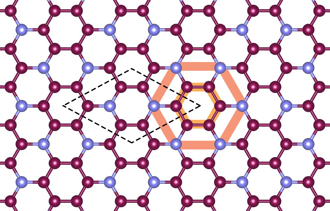
Figure 1: a) Crystal structure of C₃N monolayer. Purple and blue circles refer to carbon and nitrogen atoms, respectively. Dashed black lines show the unit cell. The orange line show the hexagonal unit cell, which can be useful to understand certain optical properties, see Sec. IV.

In this work we will employ the $\mathbf{k}\cdot\mathbf{p}$ [27, 28] approach in order to study the electronic properties of the monolayer C₃N. We obtain the materials specific parameters appearing in the $\mathbf{k}\cdot\mathbf{p}$ model from fitting it to density functional theory (DFT) band structure calculations. A similar methodology has been successfully used, e.g., for monolayers of transition metal dichalcogenides [29, 30]. In particular, since the conduction band (CB) minimum and valence band (VB) maximum are located at $\Gamma$ and $M$ points of the Brillouin zone, respectively, we obtain $\mathbf{k}\cdot\mathbf{p}$ Hamiltonians valid in the vicinity of these points. The insight given by the $\mathbf{k}\cdot\mathbf{p}$ model allows us to comment on certain optical properties as well. Moreover, we will also study the Landau level spectrum of C₃N, which, to our knowledge, has not been considered before.

This paper is organized as follows. In Sec. II we start with a short recap of the band structure obtained with the help of the density functional theory calculations. In Sec. III, effective $\mathbf{k}\cdot\mathbf{p}$ Hamiltonians at $\Gamma$and $M$ points are obtained, using symmetry groups and perturbation theory. Certain optical properties of this material are discussed in Sec. IV. In Sec. V the spectra of Landau levels for this material are calculated at the $\Gamma$ and $M$ points. Finally, our main results are summarized in Sec. VI.

II Band structure calculations

The band structure of monolayer C₃N has been calculated before at the DFT level of theory [31, 32, 25] and also using the GW approach[33, 2, 1]. The main effect of the GW approach is to enhance the band gap and this does not affect our main conclusions below. To be self-contained, we repeat the band structure calculations at the DFT level. The schematics of the crystal lattice of single-layer C₃N is shown in the Fig. 1. The lattice of C₃N possess P6/mmm space group with a planar hexagonal lattice and the unit cell contains six carbon and two nitrogen atoms. We used the Wien2K package[34] to perform first-principles calculations based on density functional theory (DFT). For the exchange-correlation potential we used the generalized gradient approximation (GGA) [35]. The optimized input parameters such as RKmax, lmax, and k-point were selected to be $8.5$, $10$, and $14\times 14\times 3$, respectively. The convergence accuracy of self-consistent calculations for the electron charge up to $0.0001$ was chosen and the forces acting on the atoms were optimized to $0.1$dyn/a.u.

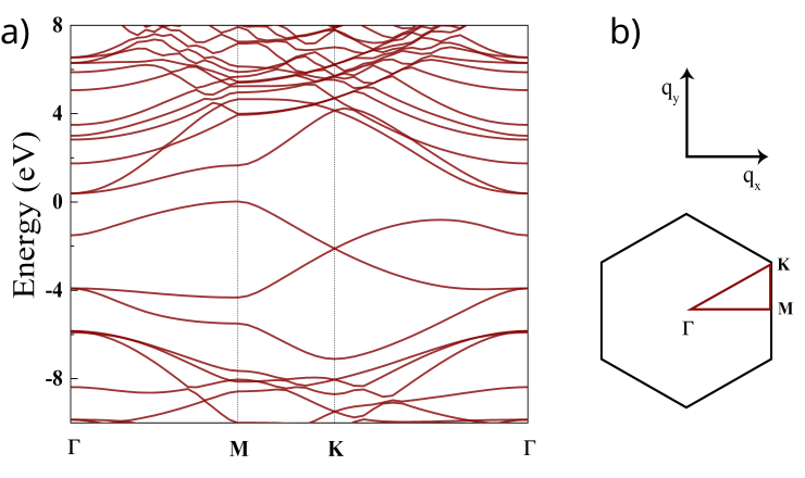
Figure 2: a) DFT band structure calculations for C₃N along the $\Gamma-K-M-\Gamma$ line in the BZ. b) orientation of the BZ and the high symmetry points $\Gamma$, $K$, $M$.

The optimized lattice constant is $a_{0}=4.86\AA{}$, in good agreement with previous studies [31, 36].

The calculated band structure is shown in Fig. 2. The conduction band minimum is located at the $\Gamma$ point, while the valence band maximum can be found at the $M$ of the BZ. Thus, at the DFT level C₃N is an indirect band gap semiconductor with a band gap of $E_{bg}=0.48$ eV which is in good agreement with previous works [21, 37]. We have checked that the magnitude of the spin-orbit coupling is small at the band-edge points of interest and therefore in the following we will neglect it. The main effect of spin-orbit coupling is to lift degeneracies at certain high-symmetry points and lines, e.g., the four-fold degeneracy of the conduction band at the $\Gamma$ point would be split into two, two-fold degenerate bands.

III Effective $\mathbf{k}\cdot\mathbf{p}$ Hamiltonians

We now introduce the $\mathbf{k}\cdot\mathbf{p}$ for the $\Gamma$ point, where the band edge of the CB is located, and for the $M$ point, where the band edge of the VB can be found.

III.1 $\Gamma$ point

The pertinent point group at the $\Gamma$ point of the BZ is $D_{6h}$. We obtained the corresponding irreducible representations of the nine bands around the Fermi level at the $\Gamma$ point with the help of the Wien2k package. Using this information one can then set up a nine bands $\mathbf{k}\cdot\mathbf{p}$ model along the lines of Ref. [30], see Appendix A for details. Here we only mention that there is no $\mathbf{k}\cdot\mathbf{p}$ matrix element between the VB and the degenerate CB, CB+1 which means that direct optical transitions are not allowed between these two bands. Since it is usually difficult to work with a nine-band Hamiltonian, we derived an effective low-energy Hamiltonian which describes the two (degenerate) conduction bands and the valence band. Using the Löwdin partitioning technique [38, 39] we find that

$$H_{\rm eff}^{\Gamma}=H_{0}^{\Gamma}+H_{\mathbf{k}\cdot\mathbf{p}}^{\Gamma},$$ (1a)

$$H_{0}^{\Gamma}=\begin{pmatrix}\varepsilon_{vb}&0&0\\ 0&\varepsilon_{cb}&0\\ 0&0&\varepsilon_{cb+1}\\ \end{pmatrix}$$ (1b)

$$H_{\mathbf{k}\cdot\mathbf{p}}^{\Gamma}=\begin{pmatrix}\alpha_{1}q^{2}&0&0\\ 0&(\alpha_{2}+\alpha_{3})q^{2}&-\alpha_{3}(q_{+})^{2}\\ 0&-\alpha_{3}(q_{-})^{2}&(\alpha_{2}+\alpha_{3})q^{2}\end{pmatrix}.$$ (1c)

Here $\varepsilon_{cb}=\varepsilon_{cb+1}=0.386$ eV and $\varepsilon_{vb}=-1.50$ eV are band edge energies of the degenerate CB minimum and VB maximum. The wavenumbers $q_{x}$, $q_{y}$ are measured from the $\Gamma$ point, $q_{\pm}=q_{x}\pm iq_{y}$ and $q^{2}=q_{x}^{2}+q_{y}^{2}$ and in $\alpha_{2}$ we took into account the free electron term[29].

Note, that there are no linear-in-$\mathbf{q}$ matrix elements between the VB and the degenerate CB, CB+1 bands. In higher order of $\mathbf{q}$ these bands do couple, but this is neglected in the minimal model given in Eq. (1c). The minimal model given in Eq. (1) already captures an important property of the degenerate CB and CB+1 bands from the DFT calculations, which is that their effective masses are different. One finds from Eq.(1c) that the effective masses are $1/m_{cb}^{\Gamma}=\frac{2}{\hbar^{2}}\alpha_{2}$ and $1/m_{cb+1}^{\Gamma}=\frac{2}{\hbar^{2}}(\alpha_{2}+2\alpha_{3})$. The material parameters $\alpha_{i}$ can be obtained, e.g., by fitting these effective masses to the DFT band structure calculations. We found that $\alpha_{1}=13.77$ eVŲ, $\alpha_{2}=5.19$ eVŲ and $\alpha_{3}=3.95$ eVŲ. The corresponding effective masses at the $\Gamma$ point are shown in Table 1.

Table 1: Effective masses at the $\Gamma$ and M points

	All directions	M - $\Gamma$ line	M - K line
$m_{vb}^{\Gamma}/m_{e}$	0.27	-	-
$m_{cb}^{\Gamma}/m_{e}$	0.73	-	-
$m_{cb+1}^{\Gamma}/m_{e}$	0.29	-	-
$m_{vb}^{M}/m_{e}$	-	-0.82	-0.12
$m_{cb}^{M}/m_{e}$	-	-0.87	0.10

III.2 M point

Next we consider the $M$ point, where the location of the VB maximum is. The relevant point group is $D_{2h}$. Since this point group has only one-dimensional irreducible representation, one expects that there are no degenerate bands near the $M$ point. This is in agreement with our DFT calculations, see Fig. 2. Because of the dense spectrum in the conduction band, we start with a $13$ bands $\mathbf{k}\cdot\mathbf{p}$ Hamiltonian (see Appendix B for details) and by projecting out the higher energy bands we obtain an effective two band model for the VB and the CB.

This effective model reads

$$H_{\rm eff}^{M}=H_{0}^{M}+H_{\mathbf{k}\cdot\mathbf{p}}^{M},$$ (2a)

$$H_{0}^{M}=\begin{pmatrix}\varepsilon_{vb}&0\\ 0&\varepsilon_{cb}\\ \end{pmatrix},$$ (2b)

$$H_{\mathbf{k}\cdot\mathbf{p}}^{M}=\begin{pmatrix}\dfrac{\hslash^{2}}{2m_{e}}q_{x}^{2}+\beta_{1}q_{y}^{2}&\gamma_{21}q_{x}\\ \gamma_{21}^{*}q_{x}&\beta_{2}q_{x}^{2}+\beta_{3}q_{y}^{2}\\ \end{pmatrix}.$$ (2c)

Here $\varepsilon_{vb}=0.021$ eV and $\varepsilon_{cb}=1.65$ eV refer to band edges energies of the VB and the CB, respectively and the $q_{x}$ direction is along the $\Gamma-M$ line. We note that $H_{\mathbf{k}\cdot\mathbf{p}}^{M}$ includes free electron term as well[29]. It is interesting to note that $H_{\mathbf{k}\cdot\mathbf{p}}^{M}$ has the same general form as the $\mathbf{k}\cdot\mathbf{p}$ model for the $\Gamma$ point of phosphorene [40, 41]. An important difference between the two cases, apart from the fact that the multiplicity of the $\Gamma$ and $M$ points are different, is that in the case of C₃N there is a saddle point in the dispersion at the $M$ points, whereas in the case of phosphorene the dispersion has a positive slope in every direction at the $\Gamma$ point. The material parameters appearing Eq. (2c) can be obtained by fitting the dispersion to the DFT band structure calculations. The range of fitting was $\%0.5$ of both the $M-K$ and $M-\Gamma$ directions. We found $\beta_{1}=-31.36$ eVŲ, $\beta_{2}=-10.02$ eVŲ, $\beta_{3}=34.87$ eVŲ, and $\gamma_{21}=3.41$ eVÅ. The corresponding effective masses are given in Table 1. One can indeed see that the effective masses have a different sign along the $M-K$ and $M-\Gamma$ directions.

IV Comments on the optical properties

Recently, Ref. [1, 2] have studied the optical properties of C₃N based on the DFT+G₀W₀ methodology to obtain an improved value for the band gap and the Bethe-Salpeter approach to calculate the excitonic properties. Several findings of Ref. [1, 2] can be interpreted with the help of the results presented in Sec. III.

According to the numerical calculations of Ref. [2], the lowest energy direct excitonic state is doubly-degenerate and dark. The corresponding electron-hole transitions are located in the vicinity of the $\Gamma$ point and the electron part of the exciton wavefunction is localized on the benzene rings of C₃N if the hole is fixed on an N atom.

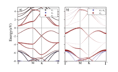
Figure 3: Atomic orbital weight of a) carbon and b) nitrogen atoms in the energy bands of C₃N monolayer.

Firstly, we note that there is no $\mathbf{k}\cdot\mathbf{p}$ matrix element between the VB and the doubly degenerate CB at the $\Gamma$ point (see Appendix A) which indicates that direct optical transitions are forbidden by symmetry. Furthermore, as shown in Fig. 3, at the $\Gamma$ point the $p_{z}$ atomic orbitals of the C atoms have a large weight in the CB, CB+1 bands and the same applies to the $p_{z}$ atomic orbitals of the N atoms in the VB. According to Table 3, the degenerate CB, CB+1 bands correspond to the two-dimensional $E_{2u}$ irreducible representation of $D_{6h}$. One can check that the following linear combinations of the $p_{z}$ atomic orbitals of the C atoms transform as the partners of the $E_{2u}$ irreducible representation:

$$\varphi_{1}=\frac{1}{\sqrt{6}}\left[p^{(1,C)}_{z}+\omega p^{(2,C)}_{z}+\omega^{2}p^{(3,C)}_{z}\right.$$

$$\qquad+\left.p^{(4,C)}_{z}+\omega p^{(5,C)}_{z}+\omega^{2}p^{(6,C)}_{z}\right],$$ (3a)

$$\varphi_{2}=\frac{1}{\sqrt{6}}\left[p^{(1,C)}_{z}+\omega^{2}p^{(2,C)}_{z}+\omega p^{(3,C)}_{z}\right.$$

$$\qquad+\left.p^{(4,C)}_{z}+\omega^{2}p^{(5,C)}_{z}+\omega p^{(6,C)}_{z}\right],$$ (3b)

where $\omega=e^{2\pi i/3}$, and $p^{(i,C)}_{z}$, $i=1,2,...,6$ denotes the $p_{z}$ orbitals of the six carbon atoms in the unit cell, see Fig. 1. Bloch wavefunctions based on $\varphi_{1}$ and $\varphi_{2}$ would indeed have a large weight on the benzene rings in each unit cell, and this helps to explain the corresponding finding of Ref. [2].

On the other hand, the $\mathbf{k}\cdot\mathbf{p}$ matrix elements are non-zero between pairs of the degenerate VB-1, VB-2 and CB, CB+1 bands, see Table 4. This means that optical transitions are allowed by symmetry and if circularly polarized light is used for excitation then $\sigma^{+}$ and $\sigma^{-}$ would excite transitions between different pairs of bands. Some of the higher energy bright excitonic states found in Ref. [2] should correspond to this transition.

At the $M$ point, on the other hand, there is finite matrix element between the VB and the CB, see Eq. (2c), which suggests that optical transitions are allowed by symmetry along the $\Gamma-M$ line. Moreover, one can expect that the optical density of states is large going from $M$ towards $\Gamma$ because the VB and the CB are approximately parallel. Note that the time reversed states can be found at $-q_{x}$, i.e., on the other side of the $\Gamma$ point. Therefore one can expect that in zero magnetic field two, degenerate bright excitonic states can be excited, and in $\mathbf{k}$ space they are localized on opposite sides of the $\Gamma$ point along the $\Gamma-M$ lines. This correspond to the findings of Ref. [2]. In external magnetic field, which breaks time reversal symmetry, the degeneracy of the two excitonic states would be broken. This is reminiscent of the valley degeneracy breaking for magnetoexcitons in monolayer TMDCs [42, 43, 44, 45, 46].

The transition along the $\Gamma-M$ line can be excited by linearly polarized light. For a general direction of the linear polarization with respect to the crystal lattice, transitions along all three $\Gamma-M$ directions in the BZ would be excited. However, when the polarization of the light is perpendicular to one of the $\Gamma-M$ line, then the interband transitions are excited only in the remaining two $\Gamma-M$ “valleys”. In contrast, when circularly polarized light is used for excitation, all three $\Gamma-M$ “valleys” are excited.

V Landau levels

We now consider the Landau levels spectrum of monolayer C₃N. Using the $\mathbf{k}\cdot\mathbf{p}$ Hamiltonians, one can employ the Kohn–Luttinger prescription, see, e.g., Ref. [39]. This means that one can replace the wavenumber $\mathbf{q}=(q_{x},q_{y})$ by the operator $\mathbf{\hat{q}}=\frac{1}{i}\nabla+\frac{e}{\hbar}\mathbf{A}$, where $e>0$ is the magnitude of electron charge and $\mathbf{A}$ is the vector potential describing the magnetic field. In the following we will use the Landau gauge and $\mathbf{A}=(0,B_{z}x,0)^{T}$. Since the components of $\mathbf{\hat{q}}$ do not commute, the Kohn–Luttinger prescription should be performed in the original nine-band ($\Gamma$ point) or thirteen-band ($M$ point) $\mathbf{k}\cdot\mathbf{p}$ Hamiltonians (see Appendices A, B) and not in the low energy effective ones given in Eq. (1) and Eq. (2c), respectively. After the Kohn–Luttinger prescription in the higher dimensional $\mathbf{k}\cdot\mathbf{p}$ model one can again use the Löwdin-partitioning to obtain low-energy effective Hamiltonians by taking care of the order of the non-commuting operators appearing in the downfolding procedure. This approach was used, e.g., in the case of monolayer TMDCs to study the valley-degeneracy breaking effect of the magnetic field [47].

V.1 Effective model at the $\Gamma$ point

The low-energy model can be expressed in terms of $\hat{q}_{\pm}=\hat{q}_{x}\pm i\hat{q}_{y}$. Note, that $\hat{q}_{+}$ and $\hat{q}_{-}$ do not commute, so that $[\hat{q}_{-},\hat{q}_{+}]=\frac{2e\mathit{B}_{z}}{\hslash}$, where $\mathit{B}_{z}$ is a perpendicular magnetic field.

$$\mathcal{H}_{\rm eff}^{\Gamma}=\mathcal{H}_{0}^{\Gamma}+\mathcal{H}^{\Gamma}(B_{z})+\mathcal{H}_{Z},$$ (4)

where $\mathcal{H}_{0}^{\Gamma}$ was defined in Eq. (1), $\mathcal{H}_{Z}=\frac{1}{2}g_{e}\mu_{b}\mathit{B}_{z}\mathit{S}_{z}$ is the Zeeman term, and

$$\mathcal{H}^{\Gamma}(B_{z})=\begin{pmatrix}\hat{\mathit{h}}_{11}&0&0\\ 0&\hat{\mathit{h}}_{22}&\hat{\mathit{h}}_{23}\\ 0&\hat{\mathit{h}}_{32}&\hat{\mathit{h}}_{33}\\ \end{pmatrix}.$$ (5)

The operators $\hat{h}_{ij}$ in $\mathcal{H}^{\Gamma}(B_{z})$ are defined as follows:

$$\hat{\mathit{h}}_{11}=\frac{1}{2m_{vb}^{\Gamma}}\left(\hat{q}_{+}\hat{q}_{-}+e\hbar B_{z}\right).$$ (6)

$$\hat{\mathit{h}}_{22}=(\alpha_{2}+\alpha_{3})\hat{q}_{+}\hat{q}_{-}+\alpha_{2}\frac{2eB_{z}}{\hbar}-\frac{\hbar eB_{z}}{2m_{e}}$$ (7a)

$$\hat{\mathit{h}}_{23}=-\alpha_{3}(\hat{q}_{+})^{2},\hskip 14.22636pt\hat{\mathit{h}}_{32}=-\alpha_{3}(\hat{q}_{-})^{2},$$ (7b)

$$\hat{\mathit{h}}_{33}=(\alpha_{2}+\alpha_{3})\hat{q}_{+}\hat{q}_{-}+\alpha_{3}\frac{2eB_{z}}{\hbar}+\frac{\hbar eB_{z}}{2m_{e}}.$$ (7c)

Here $\hat{h}_{11}$ corresponds to the VB, while the degenerate CB, CB+1 are described by the $2\times 2$ block in Eq. (5). One can introduce the creation and annihilation operators $a^{\dagger}$, $a$ by $\hat{q}_{-}=\frac{\sqrt{2}}{l_{B}}a$, $\hat{q}_{+}=\frac{\sqrt{2}}{l_{B}}a^{\dagger}$, where $l_{B}=\sqrt{\hslash/eB_{z}}$ is the magnetic length. The LLs are obtained from $\hat{\mathit{h}}_{11}$ correspond to the usual harmonic oscillator spectrum $E_{vb}^{\Gamma}=\hbar\omega_{vb}^{\Gamma}(n+1/2)$, where $\omega_{vb}=eB_{z}/m_{vb}^{\Gamma}$ and $n=0,1,2\dots$ is a positive integer.

Regarding the LLs of the degenerate CB, CB+1 bands, one can anticipate from Eq. (7) that the Landau level spectrum of this minimal model exhibits an interplay of features known from bilayer graphene and conventional semiconductors. Two eigenstates read

$$\Psi_{0}=\left(\begin{array}[]{c}|0\rangle\\ 0\end{array}\right),\hskip 14.22636pt\Psi_{1}=\left(\begin{array}[]{c}|1\rangle\\ 0\end{array}\right),$$ (8)

where $|0\rangle$ and $|1\rangle$ are harmonic oscillator eigenfunctions. The corresponding eigenvalues are $E_{0}^{\Gamma}=\alpha_{2}\frac{2eB_{z}}{\hbar}-\frac{\hbar eB_{z}}{2m_{e}}$ and $E_{1}^{\Gamma}=(2\alpha_{2}+\alpha_{3})\frac{2eB_{z}}{\hbar}-\frac{\hbar eB_{z}}{2m_{e}}$, respectively. The eigenstates in Eq. (8) have the same form as the two lowest energy eigenstates of bilayer graphene. However, the $E_{0}$ and $E_{1}$ are not degenerate and they do depend on magnetic field, unlike in the case of bilayer graphene.

The rest of the eigenvalues can be obtained by using the Ansatz

$$\Psi_{n}=\left(\begin{array}[]{c}a_{1}|n+2\rangle\\ a_{2}|n\rangle\end{array}\right),$$ (9)

where $n=0,1,2\dots$ and $a_{1}$,$a_{2}$ are constants. This Ansatz leads to a $2\times 2$ eigenvalue equation yielding the energy of two LLs for each $n$. The eigenvalues can be analytically calculated, but the resulting expression is quite lengthy and not particularly insightful.

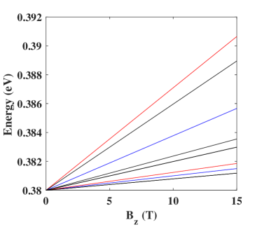
Figure 4: Landau levels in the CB at the $\Gamma$ point of the BZ as a function of the out-of-plane magnetic field $B_{z}$. Blue lines show $E_{0}^{\Gamma}$ and $E_{1}^{\Gamma}$ given below Eq. (8) and red lines indicate the first two LLs that can be obtained from the Ansatz in Eq. (9). Black lines show the ”conventional” LLs, see the text.

We plot the first four LLs as a function of magnetic field in Fig. 4. They correspond to $E_{0}^{\Gamma}$ and $E_{1}^{\Gamma}$ given below Eq. (8) and the two LLs that can be obtained using the Ansatz in Eq. (9) for $n=0$. For comparison, we also plot the energies of ”conventional” LLs $E_{n}^{cb}=\hbar\omega_{cb}^{\Gamma}(n+\frac{1}{2})$ and $E_{n}^{cb+1}=\hbar\omega_{cb+1}^{\Gamma}(n+\frac{1}{2})$, where $\omega_{cb}^{\Gamma}={eB_{z}}/{m_{cb}^{\Gamma}}$ ($\omega_{cb+1}^{\Gamma}={eB_{z}}/{m_{cb+1}^{\Gamma}}$) and the effective mass $m_{cb}^{\Gamma}$ ($m_{cb+1}^{\Gamma}$) was defined below Eq. (1). One can see that the LLs calculated using Eqs. (8) and (9) are different from the conventional LLs, which indicates the important effect of the interband coupling. In Fig. 5 we show the LL energies as a function of the LL index $n$ for a fixed magnetic field $B_{z}=10$ T. One can see that for large $n$ the LLs energies obtained from Eq. 9 (magenta dots) run parallel with the conventional LLs (black dots). This means that in this limit both set of LLs can be described by cyclotron energies $\hbar\omega_{cb}^{\Gamma}$ and $\hbar\omega_{cb+1}^{\Gamma}$, but there is an energy difference between them. However, in the deep quantum regime ($n=0,1$) the two sets of LLs cannot be characterized by the same cyclotron frequencies.

Figure 5: Landau levels in the CB at the $\Gamma$ point of the BZ as a function of the LL index n for $B_{z}=10$ T. Magenta dots indicate LLs which can be obtained from the Ansatz in Eq. (9). Black dots show the ”conventional” LLs, see the text.

We note, however, that electron-electron interactions may modify the above single particle LL picture, similarly to what has recently been found in monolayer MoS₂ [48]. Namely, the obtained effective masses of the degenerate CB and CB+1 bands are quite large, which means that the kinetic energy of the electrons is suppressed. The importance of the electron-electron interactions can be characterized by the dimensionless Wigner-Seitz radius $r_{s}=1/(\sqrt{\pi n_{e}}a_{B}^{\ast})$. Here $n_{e}$ is the electron density, $a_{B}^{\ast}=a_{B}(\kappa m_{e}/m^{\ast})$ is the effective Bohr radius, $m^{\ast}$ is the effective mass, $\kappa$ is the dielectric constant and $a_{B}$ is the Bohr radius. Taking [31] $\kappa=5$ and an electron density of $n=4\cdot 10^{12}$ cm², one finds $r_{s}=7.79$ for the heavier band, where $m^{\ast}/m_{e}=0.73$. This value of $r_{s}$ indicates that electron-electron interactions can be important. Therefore this material may offer an interesting system to study the interplay of electron-electron interactions and interband coupling.

V.2 $M$ point

We obtain the following low-energy effective Hamiltonian in terms of the operators $\hat{q}_{x}$ and $\hat{q}_{y}$:

$$\mathcal{H}_{\rm eff}^{M}=\mathcal{H}_{0}^{M}+\mathcal{H}^{M}(B_{z})+\mathcal{H}_{Z}$$ (10)

where $\mathcal{H}_{0}^{M}$ was defined in Eq. (2b) and $\mathcal{H}^{M}(B_{z})$ corresponds to Eq. (2c):

$$\mathcal{H}^{M}(B_{z})=\begin{pmatrix}\hat{\mathit{h}}_{11}&\hat{\mathit{h}}_{12}\\ \hat{\mathit{h}}_{21}&\hat{\mathit{h}}_{22}\\ \end{pmatrix},$$ (11)

where

$$\hat{\mathit{h}}_{11}=\dfrac{\hslash^{2}}{2m_{e}}\hat{q}_{x}^{2}+\beta_{1}\hat{q}_{y}^{2},$$ (12a)

$$\hat{\mathit{h}}_{12}=\gamma_{21}\hat{q}_{x},\hskip 14.22636pt\hat{\mathit{h}}_{21}=\gamma_{21}^{*}\hat{q}_{x},$$ (12b)

$$\hat{\mathit{h}}_{22}=\beta_{2}\hat{q}_{x}^{2}+\beta_{3}\hat{q}_{y}^{2}.$$ (12c)

The off-diagonal elements of $\mathcal{H}^{M}(B_{z})$ are significantly smaller then the diagonal ones for magnetic fields $B_{z}\lesssim 15$ T, therefore one can again use the Löwdin partitioning to transform them out. Since the band edge at the $M$ point is in the VB, in the following we consider the LLs in this band. By rewriting $\hat{q}_{x}$ and $\hat{q}_{y}$ in terms of annihilation and creation operators $\hat{q}_{x}=\dfrac{1}{\sqrt{2}l_{B}}(\hat{a}^{\dagger}+\hat{a})$, and $\hat{q}_{y}=\dfrac{-i}{\sqrt{2}l_{B}}(\hat{a}^{\dagger}-\hat{a})$, one finds that the LLs for VB are given by

$${E}_{n,vb}=\varepsilon_{vb}+\hslash\omega_{vb}^{M}(n+\frac{1}{2})+\dfrac{1}{2}g_{e}\mu_{b}B_{z}S_{z}.$$ (13)

Here $\omega_{vb}^{M}=\dfrac{e\mathit{B}_{z}}{2m_{vb}^{*}}$ is cyclotron frequency, where $m_{vb}=\sqrt{m_{vb,x}m_{vb,y}}$ and $m_{vb,x}$ and $m_{vb,y}$ refer to the effective masses along the $\Gamma$-$M$ and $M$-$K$ directions, see Table 1.

VI Summary

In summary, we derived effective low energy Hamiltonians for monolayer C₃N at the $\Gamma$ and $M$ points of the Brillouin zone. We showed that at the $\Gamma$ point there are no linear-in-$\mathbf{q}$ matrix elements between the VB and the degenerate CB bands, which means that optical transition are not allowed. We showed that optical transitions are allowed between the degenerate VB-1, VB-2 and the CB, CB+1 bands at the $\Gamma$ point if circularly polarized light is used. We also found that there is a saddle point in the energy dispersion of $M$ point. In addition, we suggested that the transition along the $\Gamma-M$ line can be excited by linearly polarized light at the $M$ point. Moreover, we obtained the Landau level spectra by employing the Kohn–Luttinger prescription for the $\mathbf{k}\cdot\mathbf{p}$ Hamiltonians at the $\Gamma$ and $M$ points. We pointed out the important effect of the interband coupling on the Landau level spectrum at the $\Gamma$ point. An interesting further direction could be the study of electron-electron interaction effects on the Landau level splittings, which can be important due to the heavy effective mass.

VII Acknowledgments

We thank Martin Gmitra for his technical help at the early stages of this project. This work was supported by the ÚNKP-21-5 New National Excellence Program of the Ministry for Innovation and Technology from the source of the National Research, Development and Innovation Fund and by the Hungarian Scientific Research Fund (OTKA) Grant No. K134437. A.K. also acknowledges support from the Hungarian Academy of Sciences through the Bólyai János Stipendium (BO/00603/20/11).

Appendix A Nine-band model at the $\Gamma$ point

In this Appendix, we provide some details of the nine-band $\mathbf{k}\cdot\mathbf{p}$ Hamiltonian mentioned in the main text, which is valid at $\Gamma$ point of the BZ. The small group of the $\mathbf{k}$ vector at the $\Gamma$ point is a $D_{6h}$, the character table of this point group is given in Table 2.

Table 2: Character table for $D_{6h}$ point group.

$D_{6h}$	$E$	$2C_{6}(z)$	$2C_{3}$	$C_{2}$	$3C_{2}^{{}^{\prime}}$	$3C_{2}^{"}$	$i$	$2S_{3}$	$2S_{6}$	$\sigma_{h}(xy)$	$3\sigma_{d}$	$3\sigma_{v}$	Linear functions, rotations
$A_{1g}$	+1	+1	+1	+1	+1	+1	+1	+1	+1	+1	+1	+1	-
$A_{2g}$	+1	+1	+1	+1	-1	-1	+1	+1	+1	+1	-1	-1	$R_{z}$
$B_{1g}$	+1	-1	+1	-1	+1	-1	+1	-1	+1	-1	+1	-1	-
$B_{2g}$	+1	-1	+1	-1	-1	+1	+1	-1	+1	-1	-1	+1	-
$E_{1g}$	+2	+1	-1	-2	0	0	+2	+1	-1	-2	0	0	$(R_{x},R_{y})$
$E_{2g}$	+2	-1	-1	+2	0	0	+2	-1	-1	+2	0	0	-
$A_{1u}$	+1	+1	+1	+1	+1	+1	-1	-1	-1	-1	-1	-1	-
$A_{2u}$	+1	+1	+1	+1	-1	-1	-1	-1	-1	-1	+1	+1	z
$B_{1u}$	+1	-1	+1	-1	+1	-1	-1	+1	-1	+1	-1	+1	-
$B_{2u}$	+1	-1	+1	-1	+1	-1	+1	-1	-1	+1	+1	-1	-
$E_{1u}$	+2	+1	-1	-2	0	0	-2	-1	+1	+2	0	0	$(x,y)$
$E_{2u}$	+2	-1	-1	+2	0	0	-2	+1	+1	-2	0	0	-

The Bloch wavefunctions of each band transform according to one of the irreducible representations of $D_{6h}$. This “symmetry label” of the bands can be determined, e.g., by considering which atomic orbitals have a large weight at a given $\mathbf{k}$-space point [30]. We used the corresponding output of the Wien2k code to obtain the symmetries of nine bands that we will use to set up a $\mathbf{k}\cdot\mathbf{p}$ model, see Table 3. Here VB-1, VB-2…(CB+1, CB+2…) denotes the first, second band below the VB (above the CB).

Table 3: Irreducible representations for nine bands at the $\Gamma$ point. Note, that VB-1 and VB-2 are degenerate, and they are described by the partners of the two-dimensional $E_{1g}$ representation. Similarly, CB and CB+1 are degenerate, and they are described by the partners of the two-dimensional $E_{2u}$ representation.

Band	Irreducible representation
VB-3	$B_{1g}$
VB-2	$E_{1g}$
VB-1	$E_{1g}$
VB	$A_{2u}$
CB	$E_{2u}$
CB+1	$E_{2u}$
CB+2	$A_{1g}$
CB+3	$A_{1g}$
CB+4	$A_{2u}$

One can then determine the non-zero matrix elements of the operator $\mathcal{H}=\frac{1}{2}\left(\hat{p}_{+}q+\hat{p}_{-}q_{+}\right)$, where $\hat{p}_{\pm}=\hat{p}_{x}\pm i\hat{p}_{y}$ are momentum operators, using similar arguments as in Ref. [30]. The result is given in Table 4.

Table 4: $\mathbf{k}\cdot\mathbf{p}$ matrix elements at $\Gamma$ point.

$H_{k.p}$	CB+4	CB+3	CB+2	VB-1	VB-2	VB-3	VB	CB	CB+1
CB+4	0	0	0	$\lambda_{1}q_{-}$	$\lambda_{2}q_{+}$	0	0	0	0
CB+3	0	0	0	0	0	0	0	0	0
CB+2	0	0	0	0	0	0	0	0	0
VB-1	$\lambda_{1}^{*}q_{+}$	0	0	0	0	0	$\lambda_{3}q_{+}$	0	$\lambda_{4}q_{-}$
VB-2	$\lambda_{2}^{*}q_{-}$	0	0	0	0	0	$\lambda_{5}q_{-}$	$\lambda_{6}q_{+}$	0
VB-3	0	0	0	0	0	0	0	$\lambda_{7}q_{-}$	$\lambda_{8}q_{+}$
VB	0	0	0	$\lambda_{3}^{*}q_{-}$	$\lambda_{5}^{*}q_{+}$	0	0	0	0
CB	0	0	0	0	$\lambda_{6}^{*}q_{-}$	$\lambda_{7}^{*}q_{+}$	0	0	0
CB+1	0	0	0	$\lambda_{4}^{*}q_{+}$	0	$\lambda_{8}^{*}q_{-}$	0	0	0

Some useful relations between the non-zero matrix elements of the $\mathbf{k}\cdot\mathbf{p}$ Hamiltonian can be derived by considering the symmetries of the basis functions. The degenerate VB-1, VB-2 bands transform as the $E_{1g}$ irreducible representation of $D_{6h}$ at the $\Gamma$ point, see Table 3. Similarly to the degenerate CB, CB+1 bands, the $p_{z}$ orbitals of the carbon atoms have a large weight in these bands. One can check that the following linear combinations of the $p_{z}$ atomic orbitals of the C atoms transform as the partners of the $E_{1g}$ irreducible representation:

$$\varphi_{3}=\frac{1}{\sqrt{6}}\left[p_{z}^{1,C}+\Omega p_{z}^{2,C}+\Omega^{2}p_{z}^{3,C}\right.$$

$$\qquad\left.-p_{z}^{4,C}+\Omega^{4}p_{z}^{5,C}+\Omega^{5}p_{z}^{6,C}\right]$$ (14a)

$$\varphi_{4}=\frac{1}{\sqrt{6}}\left[p_{Z}^{1,C}+\Omega^{5}p_{z}^{2,C}+\Omega^{4}p_{z}^{3,C}\right.$$

$$\qquad\left.-p_{z}^{4,C}+\Omega^{2}p_{z}^{5,C}+\Omega P_{6,C}\right]$$ (14b)

where $\Omega=e^{i\pi/3}$. For simplicity, we denote the Bloch wavefunction based on $\varphi_{i}$ by $|\varphi_{i}\rangle$. The non-zero matrix elements between the degenerate {CB,CB+1} and {VB-1,VB-2} bands are $\langle\varphi_{3}|\hat{p}_{-}|\varphi_{1}\rangle$ and $\langle\varphi_{4}|\hat{p}_{+}|\varphi_{2}\rangle$. One can easily check that $\left(\langle\varphi_{4}|\hat{p}_{+}|\varphi_{2}\rangle\right)^{*}=\langle\varphi_{3}|\hat{p}_{-}|\varphi_{1}\rangle$, where $*$ denotes complex conjugation.

We will denote the Bloch wavefunction corresponding to VB-3 by $|\varphi_{B_{1g}}\rangle$. The non-zero matrix elements between the degenerate {CB,CB+1} and VB-3 are $\langle\varphi_{B_{1g}}|\hat{p}_{+}|\varphi_{1}\rangle$ and $\langle\varphi_{B_{1g}}|\hat{p}_{-}|\varphi_{2}\rangle$. Considering the transformation properties of the Bloch wavefunctions and of $\hat{p}_{\pm}$ with respect to the $C_{2}^{{}^{\prime}}$ rotation, whose axis is perpendicular to the main, out-of-plane rotation axis, one can show that $\langle\varphi_{B_{1g}}|\hat{p}_{+}|\varphi_{1}\rangle=-\langle\varphi_{B_{1g}}|\hat{p}_{-}|\varphi_{2}\rangle$. These relations are taken into account in Table 4.

Appendix B $M$ point

In this Appendix, we explain the most important details of obtaining the $\mathbf{k}\cdot\mathbf{p}$ Hamiltonian for the $M$ point of the BZ, where the relevant point group is $D_{2h}$ . The character table for $D_{2h}$ point group is given in Table 5.

Table 5: Character table for $D_{2h}$ point group.

$D_{2h}$	$E$	$C_{2}(z)$	$C_{2}(y)$	$C_{2}(x)$	$i$	$\sigma(xy)$	$\sigma(xz)$	$\sigma(yz)$	Linear functions,rotations
$A_{g}$	+1	+1	+1	+1	+1	+1	+1	+1	-
$B_{1g}$	+1	+1	-1	-1	+1	+1	-1	-1	$R_{x}$
$B_{2g}$	+1	-1	+1	-1	+1	-1	+1	-1	$R_{y}$
$B_{3g}$	+1	-1	-1	+1	+1	-1	-1	+1	$R_{z}$
$A_{u}$	+1	+1	+1	+1	-1	-1	-1	-1	-
$B_{1u}$	+1	+1	-1	-1	-1	-1	+1	+1	$x$
$B_{2u}$	+1	-1	+1	-1	-1	+1	-1	+1	$y$
$B_{3u}$	+1	-1	-1	+1	-1	+1	+1	-1	$z$

Using information from our DFT calculation, we have assigned an irreducible representations of $D_{2h}$ to the selected thirteen bands, see Table 6.

Table 6: Irreducible representations for bands at the ${M}$ point. All bands are non-degenerate.

Band	Irreducible representation
VB-3	$B_{3u}$
VB-2	$B_{1u}$
VB-1	$B_{2g}$
VB	$B_{3g}$
CB	$A_{1u}$
CB+1	$A_{1g}$
CB+2	$B_{2u}$
CB+3	$B_{1u}$
CB+4	$B_{2u}$
CB+5	$A_{1g}$
CB+6	$B_{3g}$
CB+7	$B_{1u}$
CB+8	$B_{3g}$

Finally, one can set up the $13$-bands model given in Table 7:

Table 7: $\mathbf{k}\cdot\mathbf{p}$ matrix elements at ${M}$ point

$H_{k.p}$	VB-3	VB-2	VB-1	CB+1	CB+2	CB+3	CB+4	CB+5	CB+6	CB+7	CB+8	VB	CB
VB-3	0	0	0	$\gamma_{1}q_{x}$	0	0	0	$\gamma_{2}q_{x}$	0	0	0	0	0
VB-2	0	0	$\gamma_{3}q_{x}$	0	0	0	0	0	$\gamma_{4}q_{y}$	0	$\gamma_{5}q_{y}$	$\gamma_{6}q_{y}$	0
VB-1	0	$\gamma_{3}^{*}q_{x}$	0	0	0	$\gamma_{7}q_{x}$	0	0	0	$\gamma_{8}q_{x}$	0	0	$\gamma_{9}q_{y}$
CB+1	$\gamma_{1}^{*}q_{x}$	0	0	0	$\gamma_{10}q_{y}$	0	$\gamma_{11}q_{y}$	0	0	0	0	0	0
CB+2	0	0	0	$\gamma_{10}^{*}q_{y}$	0	0	0	0	0	0	0	0	0
CB+3	0	0	$\gamma_{7}^{*}q_{x}$	0	0	0	0	0	$\gamma_{12}q_{y}$	0	$\gamma_{13}q_{y}$	$\gamma_{14}q_{y}$	0
CB+4	0	0	0	$\gamma_{11}^{*}q_{y}$	0	0	0	$\gamma_{15}q_{y}$	0	0	0	0	0
CB+5	$\gamma_{2}^{*}q_{x}$	0	0	0	0	0	$\gamma_{15}^{*}q_{y}$	0	0	0	0	0	0
CB+6	0	$\gamma_{4}^{*}q_{y}$	0	0	0	$\gamma_{12}^{*}q_{y}$	0	0	0	$\gamma_{16}q_{y}$	0	0	$\gamma_{17}q_{x}$
CB+7	0	0	$\gamma_{8}^{*}q_{x}$	0	0	0	0	0	$\gamma_{16}^{*}q_{y}$	0	$\gamma_{18}q_{y}$	$\gamma_{19}k_{y}$	0
CB+8	0	$\gamma_{5}^{*}q_{y}$	0	0	0	$\gamma_{13}^{*}q_{y}$	0	0	0	$\gamma_{18}^{*}q_{y}$	0	0	$\gamma_{20}q_{x}$
VB	0	$\gamma_{6}^{*}q_{y}$	0	0	0	$\gamma_{14}^{*}q_{y}$	0	0	0	$\gamma_{19}^{*}q_{y}$	0	0	$\gamma_{21}q_{x}$
CB	0	0	$\gamma_{9}^{*}q_{y}$	0	0	0	0	0	$\gamma_{17}^{*}q_{x}$	0	$\gamma_{20}^{*}q_{x}$	$\gamma_{21}^{*}q_{x}$	0

References

- [1] Zhao Tang, Greis J Cruz, Yabei Wu, Weiyi Xia, Fanhao Jia, Wenqing Zhang, and Peihong Zhang. Giant narrow-band optical absorption and distinctive excitonic structures of monolayer c3 n and c3b. Physical Review Applied, 17(3):034068, 2022.
- [2] Miki Bonacci, Matteo Zanfrognini, Elisa Molinari, Alice Ruini, Marilia J Caldas, Andrea Ferretti, and Daniele Varsano. Excitonic effects in graphene-like C3N. Physical Review Materials, 6(3):034009, 2022.
- [3] Kostya S Novoselov, Andre K Geim, Sergei V Morozov, D Jiang, Y Zhang, Sergey V Dubonos, Irina V Grigorieva, and Alexander A Firsov. Electric field effect in atomically thin carbon films. science, 306(5696):666–669, 2004.
- [4] AH Castro Neto, Francisco Guinea, Nuno MR Peres, Kostya S Novoselov, and Andre K Geim. The electronic properties of graphene. Reviews of modern physics, 81(1):109, 2009.
- [5] Alexander A Balandin. Thermal properties of graphene and nanostructured carbon materials. Nature materials, 10(8):569–581, 2011.
- [6] Leonid A Falkovsky. Optical properties of graphene. In Journal of Physics: conference series, volume 129, page 012004. IOP Publishing, 2008.
- [7] Kin Fai Mak, Changgu Lee, James Hone, Jie Shan, and Tony F. Heinz. Atomically thin MoS2: A new direct-gap semiconductor. Phys. Rev. Lett., 105:136805, Sep 2010.
- [8] Qing Hua Wang, Kourosh Kalantar-Zadeh, Andras Kis, Jonathan N. Coleman, and Michael S. Strano. Electronics and optoelectronics of two-dimensional transition metal dichalcogenides. Nature Nanotechnology, 7, Nov 2012.
- [9] Xiaodong Xu, Wang Yao, Di Xiao, and Tony F. Heinz. Spin and pseudospins in layered transition metal dichalcogenides. Nature Physics, 10, May 2014.
- [10] Patrick Vogt, Paola De Padova, Claudio Quaresima, Jose Avila, Emmanouil Frantzeskakis, Maria Carmen Asensio, Andrea Resta, Bénédicte Ealet, and Guy Le Lay. Silicene: compelling experimental evidence for graphenelike two-dimensional silicon. Physical Review Letters, 108(15):155501, 2012.
- [11] Abdelkader Kara, Hanna Enriquez, Ari P Seitsonen, LC Lew Yan Voon, Sébastien Vizzini, Bernard Aufray, and Hamid Oughaddou. A review on silicene—new candidate for electronics. Surface science reports, 67(1):1–18, 2012.
- [12] Alexandra Carvalho, Min Wang, Xi Zhu, Aleksandr S Rodin, Haibin Su, and Antonio H Castro Neto. Phosphorene: from theory to applications. Nature Reviews Materials, 1(11):1–16, 2016.
- [13] Munkhbayar Batmunkh, Munkhjargal Bat-Erdene, and Joseph G Shapter. Phosphorene and phosphorene-based materials–prospects for future applications. Advanced Materials, 28(39):8586–8617, 2016.
- [14] Adil Acun, Lijie Zhang, Pantelis Bampoulis, M v Farmanbar, Arie van Houselt, AN Rudenko, M Lingenfelder, G Brocks, Bene Poelsema, MI Katsnelson, et al. Germanene: the germanium analogue of graphene. Journal of physics: Condensed matter, 27(44):443002, 2015.
- [15] Linyang Li, Xiangru Kong, Ortwin Leenaerts, Xin Chen, Biplab Sanyal, and François M Peeters. Carbon-rich carbon nitride monolayers with dirac cones: Dumbbell c4n. Carbon, 118:285–290, 2017.
- [16] Meysam Makaremi, Sean Grixti, Keith T Butler, Geoffrey A Ozin, and Chandra Veer Singh. Band engineering of carbon nitride monolayers by n-type, p-type, and isoelectronic doping for photocatalytic applications. ACS applied materials & interfaces, 10(13):11143–11151, 2018.
- [17] A Bafekry, M Faraji, MM Fadlallah, I Abdolhosseini Sarsari, HR Jappor, S Fazeli, and M Ghergherehchi. Two-dimensional porous graphitic carbon nitride c6n7 monolayer: First-principles calculations. Applied Physics Letters, 119(14):142102, 2021.
- [18] Mohammed Ismael. A review on graphitic carbon nitride (g-c3n4) based nanocomposites: synthesis, categories, and their application in photocatalysis. Journal of Alloys and Compounds, 846:156446, 2020.
- [19] Wee-Jun Ong, Lling-Lling Tan, Yun Hau Ng, Siek-Ting Yong, and Siang-Piao Chai. Graphitic carbon nitride (g-c3n4)-based photocatalysts for artificial photosynthesis and environmental remediation: are we a step closer to achieving sustainability? Chemical reviews, 116(12):7159–7329, 2016.
- [20] Javeed Mahmood, Eun Kwang Lee, Minbok Jung, Dongbin Shin, Hyun-Jung Choi, Jeong-Min Seo, Sun-Min Jung, Dongwook Kim, Feng Li, Myoung Soo Lah, Noejung Park, Hyung-Joon Shin, Joon Hak Oh, and Jong-Beom Baek. Two-dimensional polyaniline (c¡sub¿3¡/sub¿n) from carbonized organic single crystals in solid state. Proceedings of the National Academy of Sciences, 113(27):7414–7419, 2016.
- [21] Siwei Yang, Wei Li, Caichao Ye, Gang Wang, He Tian, Chong Zhu, Peng He, Guqiao Ding, Xiaoming Xie, Yang Liu, Yeshayahu Lifshitz, Shuit-Tong Lee, Zhenhui Kang, and Mianheng Jiang. C3N - a 2D crystalline, hole-free, tunable-narrow-bandgap semiconductor with ferromagnetic properties. Advanced Materials, 29(16):1605625, 2017.
- [22] Bohayra Mortazavi. Ultra high stiffness and thermal conductivity of graphene like C3N. Carbon, 118:25–34, 2017.
- [23] Yan Gao, Haifeng Wang, Maozhu Sun, Yingchun Ding, Lichun Zhang, and Qingfang Li. First-principles study of intrinsic phononic thermal transport in monolayer C3N. Physica E: Low-dimensional Systems and Nanostructures, 99:194–201, 2018.
- [24] S Kumar, S Sharma, V Babar, and Udo Schwingenschlögl. Ultralow lattice thermal conductivity in monolayer C3N as compared to graphene. Journal of Materials Chemistry A, 5(38):20407–20411, 2017.
- [25] Jun Zhao, Hui Zeng, and Xingfei Zhou. X3n (x=c and si) monolayers and their van der waals heterostructures with graphene and h-bn: Emerging tunable electronic structures by strain engineering. Carbon, 145:1–9, 2019.
- [26] Qing-Yuan Chen, Ming-yang Liu, Chao Cao, and Yao He. Anisotropic optical properties induced by uniaxial strain of monolayer c3n: a first-principles study. RSC advances, 9(23):13133–13144, 2019.
- [27] Lok C Lew Yan Voon and Morten Willatzen. The kp method: electronic properties of semiconductors. Springer Science & Business Media, 2009.
- [28] Mildred S Dresselhaus, Gene Dresselhaus, and Ado Jorio. Group theory: application to the physics of condensed matter. Springer Science & Business Media, 2007.
- [29] Andor Kormányos, Guido Burkard, Martin Gmitra, Jaroslav Fabian, Viktor Zólyomi, Neil D Drummond, and Vladimir Fal’ko. theory for two-dimensional transition metal dichalcogenide semiconductors. 2D Materials, 2(2):022001, 2015.
- [30] Andor Kormányos, Viktor Zólyomi, Neil D Drummond, Péter Rakyta, Guido Burkard, and Vladimir I Fal’Ko. Monolayer mos 2: Trigonal warping, the valley, and spin-orbit coupling effects. Physical Review B, 88(4):045416, 2013.
- [31] Xiaodong Zhou, Wanxiang Feng, Shan Guan, Botao Fu, Wenyong Su, and Yugui Yao. Computational characterization of monolayer c3n: A two-dimensional nitrogen-graphene crystal. Journal of Materials Research, 32(15):2993, 2017.
- [32] Xueyan Wang, Qingfang Li, Haifeng Wang, Yan Gao, Juan Hou, and Jianxin Shao. Anisotropic carrier mobility in single- and bi-layer c3n sheets. Physica B: Condensed Matter, 537:314–319, 2018.
- [33] Yabei Wu, Weiyi Xia, Weiwei Gao, Fanhao Jia, Peihong Zhang, and Wei Ren. Quasiparticle electronic structure of honeycomb c3n:from monolayer to bulk. 2D Materials, 6(1):015018, nov 2018.
- [34] Karlheinz Schwarz and Peter Blaha. Solid state calculations using Wien2k. Computational Materials Science, 28(2):259 – 273, 2003. Proceedings of the Symposium on Software Development for Process and Materials Design.
- [35] John P Perdew, Adrienn Ruzsinszky, Gábor I Csonka, Oleg A Vydrov, Gustavo E Scuseria, Lucian A Constantin, Xiaolan Zhou, and Kieron Burke. Restoring the density-gradient expansion for exchange in solids and surfaces. Physical review letters, 100(13):136406, 2008.
- [36] Asadollah Bafekry, Saber Farjami Shayesteh, and Francois M Peeters. C3N monolayer: Exploring the emerging of novel electronic and magnetic properties with adatom adsorption, functionalizations, electric field, charging, and strain. The Journal of Physical Chemistry C, 123(19):12485–12499, 2019.
- [37] Meysam Makaremi, Bohayra Mortazavi, and Chandra Veer Singh. Adsorption of metallic, metalloidic, and nonmetallic adatoms on two-dimensional c3n. The Journal of Physical Chemistry C, 121(34):18575–18583, 2017.
- [38] Per-Olov Löwdin. A note on the quantum-mechanical perturbation theory. The Journal of Chemical Physics, 19(11):1396–1401, 1951.
- [39] Roland Winkler. Spin-orbit coupling effects in two-dimensional electron and hole systems. Springer Tracts in Modern Physics, 191:1–8, 2003.
- [40] X. Y. Zhou, R. Zhang, J. P. Sun, Y. L. Zou, D. Zhang, W. K. Lou, F. Cheng, G. H. Zhou, F. Zhai, and Kai Chang. Landau levels and magneto-transport property of monolayer phosphorene. Scientific Reports, 5(1):12295, Jul 2015.
- [41] J. M. Pereira and M. I. Katsnelson. Landau levels of single-layer and bilayer phosphorene. Phys. Rev. B, 92:075437, Aug 2015.
- [42] David MacNeill, Colin Heikes, Kin Fai Mak, Zachary Anderson, Andor Kormányos, Viktor Zólyomi, Jiwoong Park, and Daniel C. Ralph. Breaking of valley degeneracy by magnetic field in monolayer MoSe2. Phys. Rev. Lett., 114:037401, Jan 2015.
- [43] Yilei Li, Jonathan Ludwig, Tony Low, Alexey Chernikov, Xu Cui, Ghidewon Arefe, Young Duck Kim, Arend M. van der Zande, Albert Rigosi, Heather M. Hill, Suk Hyun Kim, James Hone, Zhiqiang Li, Dmitry Smirnov, and Tony F. Heinz. Valley splitting and polarization by the Zeeman effect in monolayer MoSe2. Phys. Rev. Lett., 113:266804, Dec 2014.
- [44] Ajit Srivastava, Meinrad Sidler, Adrien V. Allain, Dominik S. Lembke, Andras Kis, and A. Imamoģlu. Valley Zeeman effect in elementary optical excitations of monolayer WSe2. Nature Physics, 11:141, Feb 2012.
- [45] G. Aivazian, Zhirui Gong, Aaron M. Jones, Rui-Lin Chu, J. Yan, D. G. Mandrus, Chuanwei Zhang, David Cobden, Wang Yao, and Xiaodong Xu. Magnetic control of valley pseudospin in monolayer WSe2. Nature Physics, 11:148, Feb 2012.
- [46] G. Wang, L. Bouet, M. M. Glazov, T. Amand, E. L. Ivchenko, Palleau E., X. Marie, and B. Urbaszek. Magneto-optics in transition metal diselenide monolayers. 2D Materials, 2(3):034002, 2015.
- [47] Andor Kormányos, Péter Rakyta, and Guido Burkard. Landau levels and Shubnikov–de Haas oscillations in monolayer transition metal dichalcogenide semiconductors. New Journal of Physics, 17(10):103006, 2015.
- [48] Riccardo Pisoni, Andor Kormányos, Matthew Brooks, Zijin Lei, Patrick Back, Marius Eich, Hiske Overweg, Yongjin Lee, Peter Rickhaus, Kenji Watanabe, Takashi Taniguchi, Atac Imamoglu, Guido Burkard, Thomas Ihn, and Klaus Ensslin. Interactions and magnetotransport through spin-valley coupled Landau levels in monolayer MoS2. Phys. Rev. Lett., 121:247701, Dec 2018.