Subsystem Trace-Distances of Two Random States

Abstract

We study two-state discrimination in chaotic quantum systems. Assuming that one of two $N$-qubit pure states has been randomly selected, the probability to correctly identify the selected state from an optimally chosen experiment involving a subset of $N-N_{B}$ qubits is given by the trace-distance of the states, with $N_{B}$ qubits partially traced out. In the thermodynamic limit $N\to\infty$, the average subsystem trace-distance for random pure states makes a sharp, first order transition from unity to zero at $f=1/2$, as the fraction $f=N_{B}/N$ of unmeasured qubits is increased. We analytically calculate the corresponding crossover for finite numbers $N$ of qubits, study how it is affected by the presence of local conservation laws, and test our predictions against exact diagonalization of models for many-body chaos.

I Introduction

The capability for storing and processing quantum information relies on the ability to discriminate between quantum states. Quantifying distinguishability of quantum states, specifically when only access to subregions is available, is thus a problem of fundamental and practical interest. In chaotic systems initially localized information is ‘scrambled’ into the many degrees of freedom of the system, and subsystem density matrices of generic pure states are nearly indistinguishable from fully thermal states. The ‘nearly’ was specified by Page for pure random states, which also serve as proxies for eigenstates of chaotic systems, in his classic paper Page (1993). There he showed that for these states the information stored in the smaller subsystem, defined as the deficit of the subsystem entanglement entropy $S_{A}$ from the maximum entropy of a fully mixed state, is on average $I_{A}\equiv\ln D_{A}-S_{A}=D^{2}_{A}/2D$. Here $D_{A}$, and $D$ are the Hilbert space dimensions of the smaller subsystem, respectively, the joint system, and corrections small in $1/D$ have been neglected. For reasonably large systems the entanglement entropy is self averaging and the average $S_{A}$ is also typical Bianchi and Donà (2019); Bianchi et al. (2021). Conservation laws generally reduce entanglement, increasing thus the capability to store information Bianchi and Donà (2019); Rigol et al. (2008); Lau et al. (2022); Ares et al. (2022); Vidmar and Rigol (2017); Nakagawa et al. (2018); Sugiura and Shimizu (2012, 2013); Murciano et al. (2022). If multiple charges are conserved, entanglement is (on average) promoted if the charges fail to commute with each other. That is, Page curves for non-commuting charges lie above that of commuting charges, as recently pointed out in Ref. Majidy et al. (2022). Morevover, in the presence of locally conserved charges, the entire charge distributions of initial states are conserved. The largest amount of information can then be stored in states with the broadest charge distribution Altland et al. (2022).

While Page’s formula provides information on subsystems, it does not give an answer to state-discrimination in fully information scrambling systems. Specifically, imagine one of two known random pure states $\rho$, $\sigma$, both composed of $N$ qubits, has been randomly selected. What is the (average) probability $P_{\rho\sigma}$ that performing an optimally chosen experiment on $N_{A}$ of the qubits we correctly identify the selected state, and how is $P_{\rho\sigma}$ affected by conservation laws? In this paper we want to investigate these questions, and the outline is as follows: We start briefly reviewing in Section II the concepts of the trace-distance $D_{1}$, its generalization the Schatten $n$-distances $D_{n}$, Page states, and the calculation of $D_{1}$ from $D_{n}$ via the replica trick. We then discuss in Section III the combinatorics involved in the calculation of average subsystem Schatten $n$-distances of random pure states. In Section IV we analyze the average subsystem trace-distances of random pure states and consequences of local conservation laws. We conclude in Section V with a summary and discussion, and give further technical details in the Appendices.

II Schatten-distances, Page states, and replica trick

Optimal quantum state discrimination is generally challenging, and the only completely analyzed case is for two states, see e.g. Ref. Bae and Kwek (2015) for a review. The trace-distance provides a natural metric for two-state discrimination. According to the Holevo–Helstrom theorem the best success probability for the latter is encoded in the $1$-Schatten- or trace-distance as $P_{\rho\sigma}=\frac{1}{2}\left(1+D_{1}(\rho,\sigma)\right)$ foo (a). General Schatten $n$-distances here are defined as $D_{n}(\rho,\sigma)\equiv\frac{1}{2^{1/n}}||\rho-\sigma||_{n}$, with $n$-norm of a matrix $\Lambda$ determined by its singular values $\lambda_{i}$ as $||\Lambda||_{n}=\left(\sum_{i}\lambda^{n}_{i}\right)^{1/n}$ foo (b). Notice that all Schatten distances are symmetric in the inputs, positive semi-definite, equal to zero if and only if inputs are identical, and obey the triangular inequality. That is, they all satisfy the properties of a metric, with normalization here chosen such that $0\leq D_{n}\leq 1$. Our focus here is on two-state discrimination and we thus concentrate on the $1$-distance.

Consider then a $D$-dimensional Hilbert space with entanglement-cut bi-partitioning the total system into subsystems $A$, $B$ of dimensions $D_{A}$ and $D_{B}$, respectively, with $D_{A}D_{B}=D$. Without much loss of generality, we focus here on $N$ qubit systems parametrized by $(a,b)$, where the $N_{A}$-bit vector $a$ labels the $D_{A}=2^{N_{A}}$ states of subsystem $A$ and $b$ the $D_{B}=2^{N_{B}}$ states of $B$, with $N_{B}=N-N_{A}$. Following Page, we then consider two random pure states $|\psi^{\alpha}\rangle=\sum_{a,b}\psi^{\alpha}_{ab}|a,b\rangle$, $\alpha=\rho,\sigma$, with Gaussian distributed complex amplitudes $\psi^{\alpha}_{ab}$, chosen to have zero mean and variances

$$\langle\psi_{ab}^{\alpha}\bar{\psi}_{cd}^{\beta}\rangle =\frac{1}{D}\delta_{ac}\delta_{bd}\delta_{\alpha\beta}.$$ (1)

$|\psi^{\alpha}\rangle$ describe infinite temperature thermal states of generic chaotic systems, and using Eq. (1) we employ that correlations induced by the normalization constraint are negligible for reasonable large systems $D\gg 1$. Tracing out subsystem $B$, information is lost and mixedness of the reduced density matrices,

$$\rho_{A} ={\rm tr}_{B}(|\psi^{\rho}\rangle\langle\psi^{\rho}|),\quad\sigma_{A}={\rm tr}_{B}(|\psi^{\sigma}\rangle\langle\psi^{\sigma}|),$$ (2)

increases with the number of partially traced qubits $N_{B}$.

To find trace-distances of Eq. (2) we employ the replica trick recently discussed in Ref. Zhang et al. (2019). We first calculate Schatten-distances for general even integer $n$, analytically continue to real $n$, and finally take the limit $n$ to unity,

$$\langle D_{1}(\rho_{A},\sigma_{A})\rangle =\frac{1}{2}\lim_{n\to 1}\langle{\rm tr}\left(\rho_{A}-\sigma_{A}\right)^{n}\rangle.$$ (3)

Restricting to even integers here is important, since corresponding expression for odd integers vanish (see also below), and a replica limit for the latter is thus trivially zero Zhang et al. (2019). Expanding powers in Eq. (3), we are confronted with the averages

$$\langle{\rm tr}_{A}(\rho_{A}-\sigma_{A})^{n}\rangle$$

$$\,\,={\rm sgn}(\sigma)\langle\psi_{a^{1}b^{1}}^{\alpha_{1}}\bar{\psi}_{a^{2}b^{1}}^{\alpha_{1}}\psi_{a^{2}b^{2}}^{\alpha_{2}}\bar{\psi}_{a^{3}b^{2}}^{\alpha_{2}}\cdot\cdot\cdot\psi_{a^{n}b^{n}}^{\alpha_{n}}\bar{\psi}_{a^{1}b^{n}}^{\alpha_{n}}\rangle,$$ (4)

where sums over repeated indices $\alpha_{i}=\rho,\sigma$, $a_{i}=1,..,D_{A}$, $b_{i}=1,...,D_{B}$ are implicit, and the sign-factor is ${\rm sgn}(\sigma)=\pm 1$ if an even/odd number of density matrices $\sigma_{A}$ is involved in the product. Following previous works Monteiro et al. (2021) the bookkeeping of index configurations entering the products is conveniently done in a tensor network representation shown in Fig. 1. The solid lines here indicate how the indices of matrices $\left(\psi\bar{\psi}\right)^{\alpha\beta}_{ab;a^{\prime}b^{\prime}}=\psi^{\alpha}_{ab}\bar{\psi}^{\beta}_{a^{\prime}b^{\prime}}$ are constrained due to matrix multiplication in subspace $A$, subsystem-traces over $B$, and state indices $\alpha=\rho,\sigma$, respectively (see also figure caption). Further constraints then arise from Gaussian averages Eq. (1). These are indicated by the red lines, keeping track of Hilbert space and state indices after contractions. For Page states, each of the $n!$ contributions resulting from the Gaussian averages of the $2n$ complex amplitudes in Eq. (II) is weighted by an overall factor $1/D^{n}$, and terms can be organized according to the numbers of free subspace summations, or ‘cycles’, as we discuss next.

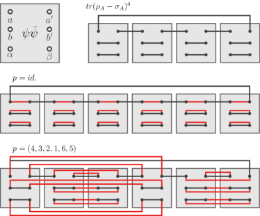
Figure 1: Tensor network representation of averages Eq. (II). Top left: Representation of a pair of amplitudes from the expansion $\alpha_{A}=\sum_{a,a^{\prime}}\sum_{b}\psi^{\alpha}_{ab}\bar{\psi}^{\alpha}_{a^{\prime}b}|a\rangle\langle a^{\prime}|$, with $\alpha=\rho,\sigma$. Each dot represents an index to be contracted, and contractions must be between right- and left-side indices. Top right: Structure of $\mathrm{tr}(\rho_{A}-\sigma_{A})^{4}$, with black lines representing index contractions resulting from matrix multiplication in subspace $A$ (top line), traces in subspace $B$ (middle line), and state indices $\alpha=\rho,\sigma$ (bottom line). Notice that the index structure of states follows that of subspace $B$. When averaging the trace we only consider leading order contributions in $1/D$ resulting from non-crossing permutations. Gaussian averages then impose further contractions upon the structural ones, indicated by the red lines. Middle: Resulting index structure for $n=6$ and identity permuation $p=id$. This establishes six $B$-cycles each consisting of one element, i.e. in the notation of main text $\Lambda_{6}=(1^{6},2^{0},3^{0},4^{0},5^{0},6^{0})$. Bottom: Another example of a non-crossing permutation for $n=6$, $p=(4,3,2,1,6,5)$. This permutation establishes three $B$-cycles each consisting of two elements, $\Lambda_{6}=(1^{0},2^{3},3^{0},4^{0},5^{0},6^{0})$. In the middle diagram, contributions from states $\rho$ (positive sign) and $\sigma$ (negative sign) sum to zero in each of the one-element cycles. In the bottom diagram contributions from $\rho$ and $\sigma$ both come with positive sign and sum to two, i.e. contributions from the three cycles add up to $2^{3}=8$.

III Combinatorics of averages

It is instructive to first focus on the contribution involving only a single state density matrix, say $\rho_{A}$,

$$\langle\mathrm{tr}_{A}(\rho_{A}^{n})\rangle =\langle\psi^{\rho}_{a^{1}b^{1}}\bar{\psi}^{\rho}_{a^{2}b^{1}}\psi^{\rho}_{a^{2}b^{2}}\dots\psi^{\rho}_{a^{n}b^{n}}\bar{\psi}^{\rho}_{a^{1}b^{n}}\rangle.$$ (5)

These averages have been recently discussed in the context of the entanglement entropy foo (c), and the main observations are Penington et al. (2019); Liu and Vardhan (2020): (i) the $n!$ contributions resulting from the average of $2n$ Gaussian distributed complex variables can be organized as a sum over the permutation group $\langle\mathrm{tr}_{A}(\rho_{A}^{n})\rangle=\frac{1}{D^{n}}\sum_{p\in S_{n}}D_{A}^{C(\pi^{-1}\circ p)}D_{B}^{C(p)}$, where $C(p)$ is the number of cycles in the permutation $p$ and $\pi$ defined by $\pi(i)=(i+1){\rm mod}(n)$, (ii) the maximal number of cycles is $C(\pi^{-1}\circ p)+C(p)=n+1$ and is realized by the non-crossing permutations, (iii) their combinatorics is encoded in the Narayana numbers $N(n,k)$ where $k$ the number of cycles in $B$, and (iv) contributions of crossing permutations are suppressed in powers of $1/D$. Neglecting the latter, one thus arrives at $\langle\mathrm{tr}_{A}(\rho_{A}^{n})\rangle=\frac{1}{D^{n}}\sum_{k=1}^{n}N(n,k)D_{A}^{n-k+1}D_{B}^{k}$, which can be further organized in power-series defining hypergeometric functions. The calculation of Eq. (5) has thus been succeeded once the Narayana numbers have been identified as the combinatorial coefficients summing all possible non-crossing permutations of the $n$ elements containing $k$ $B$-cycles.

To extend the calculation to all terms Eq. (II) we introduce the Kreweras numbers,

$${\rm Krew}(\Lambda_{n}) =\frac{n!}{\lambda_{1}!...\lambda_{n}!(n+1-l(\Lambda_{n}))!},$$ (6)

with $l(\Lambda_{n})\equiv\sum_{i=1}^{n}\lambda_{i}$. They count the number of non-crossing permutations composed of $\lambda_{i}$ $B$-cycles formed of $i$ elements, $\Lambda_{n}=(1^{\lambda_{1}},2^{\lambda_{2}},...,n^{\lambda_{n}})$, and thus provide more detailed information than the Narayana numbers Kreweras (1972); Simion (2000). Specifically, Narayana numbers sum all Kreweras numbers specified by $l(\Lambda_{n})=k$ and $\sum_{i=1}^{n}i\lambda_{i}=n$ (see also Appendix A). With this additional information we are now ready to tackle the combinatorics required for the calculation of average Schatten $n$-distances.

Cycles in Eq. (II) can be formed from states $\rho$ or $\sigma$. Both contribute the same in absolute value, however, not always with same sign. That is, while the sign is always positive for $\rho$-cycles it alternates for $\sigma$-cycles depending on whether the number of elements involved in the cycle is even/odd foo (d). For permutations with odd element cycles the contributions from $\rho$-cycles and $\sigma$-cycles thus cancel, and therefore only those consisting of even elements contribute. Noting that $b$-indices follow that of state-indices (see also Fig. 1) we arrive at the same conclusion for $B$-cycles. That is, for non-crossing permutations with $k$ $B$-cycles only $\Lambda_{n}=(1^{0},2^{\lambda_{2}},3^{0}...,n^{\lambda_{n}})$ with all cycles composed of even elements contribute, and summing the two choices $\alpha=\rho,\sigma$ for each of the $k$ cycles adds up to a factor $2^{k}$. As a corollary we notice that moments in Eq. (II) involving odd powers $n$ vanish, as anticipated above. We are then left with the combinatorical task of counting the number of $k$-cycles consisting only of even elements. Summing the corresponding Kreweras numbers (see Appendix A for details), we find

$$N_{e}(n,k) =\frac{2}{n}\binom{n/2}{k}\binom{n}{k-1}.$$ (7)

IV Average trace-distances

Joining parts, we find the average Schatten $n$-distances of two random Page states $\langle D_{n}(\rho_{A},\sigma_{A})\rangle=\frac{1}{2D^{n}}\sum_{k=1}^{n/2}2^{k}N_{e}(n,k)D_{A}^{n-k+1}D_{B}^{k}$, which can be organized into a hypergeometric function (see Appendix B for details). For the latter the replica limit can be taken, and we arrive at the average trace-distance of two random Page states,

$$\langle D_{1}(\rho_{A},\sigma_{A})\rangle =\begin{cases}1-\frac{1}{4x},&\quad x\geq 1,\\ \frac{8\sqrt{x}}{3\pi}\,{\cal F}(x),&\quad x\leq 1,\end{cases}$$ (8)

where $x=\frac{D_{A}}{2D_{B}}$, and ${\cal F}(x)={}_{2}F_{1}(\frac{1}{2},-\frac{1}{2},\frac{5}{2},x)$ a hypergeometric function. Similar results have been recently derived in Ref. Kudler-Flam et al. (2021) using free probability techniques, and Eq. (8) agrees with their asymptotic expressions.

Fig. 2 shows the trace-distance of Page states for different numbers of qubits $N$ (solid lines) as a function of the fraction $f\equiv N_{B}/N$ of partially traced qubits, and $x=\frac{1}{2}D^{1-2f}$. Increasing $N$, one observes a sharp transition from $\langle D_{1}\rangle\simeq 1$ to $\langle D_{1}\rangle\simeq 0$ once the partially traced system contains more than half of all qubits, $f>1/2$, where ‘$\simeq$’ indicates equality up to corrections ${\cal O}(1/D)$ exponentially small in the number of qubits. In the thermodynamic limit, this becomes a first order transition, describing the emergence of self-averaging of the reduced density matrix of random pure states once more than half of the qubits are partially traced out. Two-state discrimination of Page states for $N\to\infty$ is therefore possible with unit probability $P_{\rho\sigma}=1$ if the measurement is performed on more than half of the qubits, but becomes essentially impossible, $P_{\rho\sigma}=1/2$, for measurements involving fractions smaller than half of the qubits. Finite $N$ curves all intersect in $f=1/2$, and the probability for two-state discrimination using measurements on half of the qubits is $P_{\rho\sigma}=\frac{5\pi+4}{8\pi}\simeq 0.78$, in agreement with previous work Ref. Puchała et al. (2016). Expanding the trace-distance around $f=1/2$ one finds $\langle D_{1}\rangle\simeq\frac{4+\pi}{4\pi}+\frac{1}{4}(D^{1-2f}-1)$, i.e. the probability of two-state discrimination decays with the number of unmeasured qubits as $P_{\rho\sigma}={\rm const.}-N\ln 2/4\times(1-2f)$. At $f=1$ the trace-distance is trivially zero for any realization of states, while Eq. (8) predicts a value ${\cal O}(1/\sqrt{D})$, of the same order as the value at $f=1-1/N$. The erroneous finite value at $f=1$ reflects that Page states Eq. (1) realize state-normalization only on average, rather than for each realization. We next turn to a discussion on the consequences of local conservation laws.

Conservation laws

Page’s random pure states describe generic quantum states in chaotic systems lacking any structure e.g. induced by conservation laws. For these information scrambling is most efficient, and we next discuss how local conservation of scalar charges, e.g. particle number, uni-axial magnetization, etc., affects two-state discrimination in chaotic systems. More specifically, we consider the presence of a single, extensive conserved scalar operator $\hat{Q}$ that is subsystem additive: A partition of the system into the two subsystems $A$ and $B$ implies a decomposition $\hat{Q}=\hat{Q}_{A}+\hat{Q}_{B}$, and eigenstates $\hat{Q}|n\rangle=Q(n)|n\rangle$ can be labeled by $n=(a,b)$ with $Q(n)=Q_{A}(a)+Q_{B}(b)$. It is then convenient to introduce the spectral distribution of $\hat{Q}$, $F(Q)\equiv D\Omega(Q)=\sum_{n}\delta_{Q,Q(n)}$, and corresponding subsystem spectral densities, $F_{S}(Q_{S})\equiv D_{S}\Omega_{S}(Q_{S})$, with $S=A,B$. For most cases we can assume that (except from the far tails of the spectrum irrelevant for our considerations) the unit normalized spectral densities are well approximated by Gaussians,

$$\Omega(Q) =\Omega(Q,N)=\frac{1}{\sqrt{2\pi\gamma^{2}N}}e^{-\frac{Q^{2}}{2\gamma^{2}N}},$$ (9)

with $\gamma$ some $N$-independent scale, and correspondingly for subsystem densities $\Omega_{S}(Q_{S})=\Omega(Q_{S},N_{S})$. For convenience we here choose $Q=0$ as the value with largest spectral weight.

Focusing then on the two-state discrimination of charge eigenstates, we substitute the average for Page states, Eq. (1), for the symmetry refined version,

$$\langle\psi^{\alpha}_{ab}\bar{\psi}^{\beta}_{cd}\rangle =\frac{1}{F(Q)}\delta_{Q_{A}(a)+Q_{B}(b),Q}\delta_{ac}\delta_{bd}\delta_{\alpha\beta}.$$ (10)

Eq. (10) describes random wave functions in the subspace of dimension $F(Q)$ fixed by total charge $Q$, and $\delta_{Q_{A}(a)+Q_{B}(b),Q}$ introduces non trivial correlations between the subsystems. We first concentrate on the value with largest spectral weight $Q=0$ for which the most universal behaviour can be expected. Following then the previous calculation for Page states, we find (see Appendix C for details)

$$\langle D_{1}(\rho_{A},\sigma_{A})\rangle =\begin{cases}1-\frac{1}{4x\sqrt{2f}},&x\geq 1,\\ \frac{8\sqrt{x_{f}}}{3\pi}{\cal G}(x_{f},f),&x\leq 1,\end{cases}$$ (11)

where we introduced $x_{f}\equiv x\sqrt{f/(1-f)}$ with $x=\frac{D_{A}}{2D_{B}}$ as before, and ${\cal G}(x,f)=\frac{3\pi}{4}\sum_{k=0}^{\infty}c_{k}x^{k}\binom{1/2}{k}\binom{1}{k+3/2}$ with $c_{k}=\left((1+2k)f+1/2-k\right)^{-1/2}$. As anticipated, the result Eq. (11) is unviversal in the sense that it only depends on the numbers of qubits $N$, $N_{B}$.

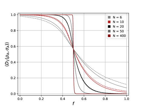
Figure 2: Average trace-distance of pure random states, Eq. (8), (solid lines) and charge eigenstates for $Q=0$, Eq. (11), (dashed lines) as functions of the relative number of traced qubits $f\equiv N_{B}/N$. System sizes are $N=6,10,20,50,400$.

Fig. 2 shows the trace-distance between two random charge eigenstates states, Eq. (11), for different numbers of qubits $N$ (dashed lines) as a function of the fraction $f\equiv N_{B}/N$ of partially traced qubits. Differences between trace-distances of charge eigenstates and Page states are notable for small systems sizes. They are most pronounced for $f\to 1/N$ and $f\to 1-1/N$, with charge eigenstates slightly above, respectively, below that of structureless Page states foo (e). At half-partition $f=1/2$, $x_{f}=x$ and ${\cal G}(x,f)={\cal F}(x)$, and trace-distances of eigenstates of charges with largest spectral weight and Page states are thus identical. This contrasts the entanglement entropy, for which the largest difference between Page and corresponding charge eigenstates are at half partition Bianchi and Donà (2019); Lau et al. (2022); Monteiro et al. (2021).

Turning to eigenstates at finite charges $Q$ different from the value of largest spectral weight, we focus on trace-distances at half-partition $f=1/2$ and the limits $f\to 1/N$, respectively, $f\to 1-1/N$. For $f=1/2$ we find a weak non-monotonous $Q$-dependence of the average trace-distance of charge eigenstates. Starting at the value $\langle D_{1}\rangle\simeq 0.57$ at $Q=0$, it increases to a maximum value $\langle D_{1}\rangle\simeq 0.58$ at $Q=\gamma\sqrt{N}$, before converging to the value $\langle D_{1}\rangle\simeq 0.50$ as $Q$ is further increased. In the limit $f\to 1/N$ we find that the average trace-distances decreases with $Q$ as $\langle D_{1}\rangle-1\sim-(\sqrt{N}/D)e^{Q^{2}/2\gamma^{2}N}$, while the leading $Q$-dependence for $f\to 1-1/N$ is given by $\langle D_{1}\rangle\sim(N^{1/4}/\sqrt{D})e^{Q^{2}/4\gamma^{2}N}$. In both limits this corresponds to a substitution of $D_{S}\mapsto F_{S}(Q)$ in the result for Page states, accounting for the reduced phase space volume of charge eigenstates (see Appendix C for more detailed expression).

Numerical analysis

Fig. 3 shows a comparison of the analytical predictions Eqs. (8) and (11) with numerical results obtained from exact diagonalization of Hamiltonians generating many-body chaos. The left panel shows eigenstates of an Sachdev-Ye-Kitaev (SYK) model with all-to-all interaction Sachdev and Ye (1993); Kit , $\hat{H}_{\rm SYK}=\frac{1}{4!}\sum_{i,j,k,l=1}^{N}J_{ijkl}\hat{\chi}_{i}\hat{\chi}_{j}\hat{\chi}_{k}\hat{\chi}_{l}$, and the right pannel of a spin-$1/2$ Ising chain with nearest neighbor interaction and longitudinal and transversal fields Kim and Huse (2013); Kim et al. (2014); Zhang et al. (2015), $\hat{H}_{S}=\sum_{i=1}^{N}\left(g\hat{\sigma}_{i}^{x}+h\hat{\sigma}_{i}^{z}+J\hat{\sigma}_{i}^{z}\hat{\sigma}_{i+1}^{z}\right)$, and periodic boundary condition $\sigma_{N+1}^{z}=\sigma_{1}^{z}$. Here $\{\hat{\chi}_{l}\}$ are Majorana operators and $\{\hat{\sigma}_{i}^{x},\hat{\sigma}_{i}^{z}\}$ Pauli matrices. In both cases we have chosen eigenstates from the center of the band, to calculate their subsystem trace distances foo (f). In the SYK-model we average over $50$ realizations of couplings $J_{ijkl}$ (respectively $10$ for the largest system size), randomly drawn from a Gaussian distribution with vanishing mean and variance $\langle|J_{ijkl}|^{2}\rangle=6J^{2}/N^{3}$ where we set $J=2/\sqrt{N}$. For the spin chain we follow Ref. Kim and Huse (2013); Kim et al. (2014); Zhang et al. (2015), and use parameters $(g,h,J)=(0.9045,0.8090,1.0)$ for which the sytem has been shown to be thermalizing for small system sizes. Since $\hat{H}_{S}$ is translational invariant, we first block diagonalize and then average over $7$ eigenstates from a given momentum sector with energies near the band center, see also Appendix D for further details.

The SYK model lacks local conservation laws, and we find excellent agreement with Eq. (8) for Page states. For the spin chain with short-range interaction, on the other hand, energy is locally conserved and has to be taken into account as a locally conserved charge. Notice that translational invariance also implies conservation of momentum. This is, however, not subsystem additive and thus does not count as a locally conserved charge. Rather, we restrict to a given momentum sector, as described above, and then find good agreement with Eq. (11) for systems with a single conserved charge that is subsystem additive. Deviations from analytical predictions are larger for the spin chain, which we relate to eigenstates in the average that are not at energies with largest spectral weight and deviations of the density of states from Eq. (9). Overall the agreement with our analytical predictions for subsystem trace distances in absence and presence of locally conserved scalar charges, Eqs. (8) and (11), is very good even for the smallest systems with Hilbert-space dimensions $D=2^{6}$.

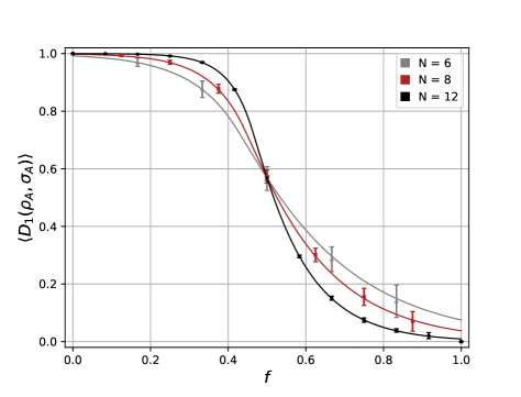
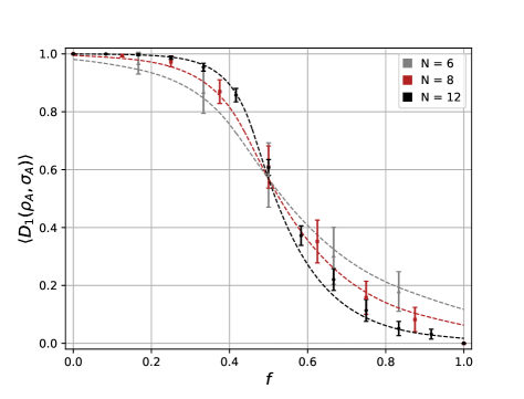
Figure 3: Left: Comparison of analytical prediction Eq. (8) (solid lines) and numerical simulations of the SYK model (symbols), here for systems of $N=14,18$ and $26$ Majorana fermions, corresponding to $N=6,8$ and $12$ qubit systems, viz., the fermion occupations in even parity sector. Right: Comparison of analytical prediction Eq. (11) (dashed lines) and numerical simulations of the spin-$1/2$ Ising chain discussed in the main text (symbols), here for $N=6$, $8$ and $12$ spins. Error bars indicate standard deviation, and for deviations at $f=1$, where $\langle D_{1}\rangle=0$, see discussion in main text.

V Summary and Discussion

We have studied two-state discrimination in chaotic quantum systems. Assuming that one of two generic $N$-qubit random pure states $\rho$, $\sigma$ has been randomly selected, we investigated the average two-state discrimination probability $P_{\rho\sigma}=\frac{1}{2}\left(1+D_{1}(\rho_{A},\sigma_{A})\right)$ that the selected state is correctly identified from an optimally chosen experiment on $N_{A}=N-N_{B}$ of the qubits. Here $D_{1}(\rho_{A},\sigma_{A})$ are the subsystem trace distances of random pure states with $N_{B}$ of the qubits partially traced out. In the thermodynamic limit $N\to\infty$, the latter makes a sharp, first order transition from unity to zero at $f=1/2$, as the fraction $f=N_{B}/N$ of unmeasured qubits is increased. We have given closed analytic expression for the corresponding crossover at finite system sizes $N$, valid up to corrections small in $1/D$.

We further studied the consequences of local conservation laws on two-state discrimination. Specifically, we calculated the average subsystem trace-distances for eigenstates of a single conserved scalar charge. Focusing on the charge $Q=0$ with largest spectral weight we obtained a closed universal expression for the trace distance that only depends on the numbers of qubits $N$, $N_{B}$. We found that state discrimination at the specific point $f=1/2$, i.e. involving measurements on half of the qubits, is not affected by local conservation laws and the same as for Page states. Away from this point, state discrimination in the presence of conservation laws becomes less/more likely than in absence of the latter for measurements involving more/less than half of the qubits. For eigenstates of general charges $Q$, state discrimination at $f=1/2$ shows a weak non-monotonous behavior as $Q$ is varied, while the behavior for different values of $f$ is similar as for $Q=0$, as we checked in the limits $f\to 1/N$ and $1-1/N$, respectively. In all cases, the probability for two-state discrimination involving local measurements on non-extensive fractions of the $N$ qubits is 1/2 up to corrections $1/D$ for Page states, respectively, $1/F(Q)$ for charge eigenstates. The exponentially small trace-distance for $f\sim{\cal O}(1)$ is expected from Eigenstate Thermalization Hypothesis (ETH) Srednicki (1994); Rigol et al. (2008); Kaufman et al. (2016), and also in accordance with subsystem ETH, its refined formulation applicable if the entire reduced density matrix appears thermal Dymarsky et al. (2018). The trace distance bounds other measures for distinguishability of quantum states, such as the relative entropy and fidelity via Pinsker’s and Fuchs-van de Graaf’s inequalities, respectively. Similar results e.g. for the consequences of conservation laws on the latter may thus be expected.

We tested our predictions against exact diagonalization of Hamiltonians for many-body chaotic systems. Specifically, we numerically calculated subsystem trace distances of eigenstates of the SYK model, lacking any local conservation laws, and an Ising spin chain with local energy conservation, respectively, and found in both cases very good agreement with our analytial predictions.

We here focused on charge eigenstates and generalizations to other pure states in chaotic systems with locally conserved charges Nakagawa et al. (2018); Sugiura and Shimizu (2012, 2013) should be interesting. Based on recent work Altland et al. (2022), we expect that pure states conditioned by broad charge distributions can be discriminated by local measurements (i.e. with probability not exponentially small in $N$) even in the presence of strong information scrambling. Finally, our results may be interesting in the context of the black hole information paradox. Specifically, one may verify whether the analogy between fixed-area states and random tensor networks, encountered for the entanglement entropy Penington et al. (2019), continues to hold for two-state discrimination of black hole micro-states.

Acknowledgments:—We thank Fernando de Mello for discussions. T. M. acknowledges collaborations with Alex Altland and David Huse on related topics, and financial support by Brazilian agencies CNPq and FAPERJ. J. T. M. acknowledges financial support by Brazilian agency CAPES.

Appendix A Summing Kreweras numbers

From Kreweras to Narayanas:—It is instructive to first review how Narayana numbers result from summing Kreweras numbers $\Lambda_{n}$ with a fixed number of cycles $l(\Lambda_{n})=k$. Substituting the explicit expression discussed in the main text, we can organize this counting as

$$N(n,k) =\sum_{\lambda_{1}=0}^{\infty}\sum_{\lambda_{2}=0}^{\infty}\cdot\cdot\cdot\sum_{\lambda_{n}=0}^{\infty}\frac{n!\,\delta_{\sum_{i=1}^{n}\lambda_{i},k}\,\delta_{\sum_{i=1}^{n}i\lambda_{i},n}}{(n-k+1)!\lambda_{1}!\lambda_{2}!...\lambda_{n}!},$$ (12)

where the two Kronecker-deltas fix the number of cycles to $k$ and total number of elements to $n$, respectively. Implementing the latter in terms of integrals $\delta_{x,n}=\frac{1}{2\pi}\int_{0}^{2\pi}e^{i(x-n)\phi}d\phi$, we exchange integration and summation and arrive at,

$$N(n,k) =\frac{n!}{(n-k+1)!}\oint\frac{dz}{2\pi i}\oint\frac{dw}{2\pi i}\frac{e^{z(w+w^{2}+...+w^{n})}}{z^{k+1}w^{n+1}},$$ (13)

which, performing pole integrals gives

$$N(n,k) =\frac{\left(\partial_{w}^{n}(w+w^{2}+...+w^{n})^{k}\right)|_{w=0}}{k!(n-k+1)!}.$$ (14)

Summing the finite geometric series one then arrives, upon performing the $n$ fold derivative and setting $w=0$, at the Narayana numbers

$$N(n,k) =\frac{1}{n}\binom{n}{k}\binom{n}{k-1}.$$ (15)

From Kreweras to ‘even-element’ Narayanas:—We can now extend the calculation to Kreweras numbers $\Lambda_{n}=(1^{0},2^{\lambda_{2}},3^{0}...,n^{\lambda_{n}})$, for which all cycles are composed of even elements,

$$N_{e}(n,k) =\sum_{\lambda_{2}=0}^{\infty}\sum_{\lambda_{4}=0}^{\infty}\cdot\cdot\cdot\sum_{\lambda_{n}=0}^{\infty}\frac{n!\,\delta_{\sum_{i=1}^{n}\lambda_{i},k}\,\delta_{\sum_{i=1}^{n}i\lambda_{i},n}}{(n-k+1)!\lambda_{2}!\lambda_{4}!...\lambda_{n}!},$$ (16)

where $n$ is even. Proceeding then as previously, we find

$$N_{e}(n,k) =\frac{n!}{(n-k+1)!}\oint\frac{dz}{2\pi i}\oint\frac{dw}{2\pi i}\frac{e^{z(w^{2}+w^{4}+...+w^{n})}}{z^{k+1}w^{n+1}},$$ (17)

which performing pole integrals gives,

$$N_{e}(n,k) =\frac{\left(\partial_{w}^{n}(w^{2}+w^{4}+...+w^{n})^{k}\right)|_{w=0}}{k!(n-k+1)!}.$$ (18)

Summing again the finite geometric series, performing the $n$ fold derivative and setting $w=0$, one then arrives at the ‘even-element’ Narayana numbers,

$$N_{e}(n,k) =\frac{2}{n}\binom{n/2}{k}\binom{n}{k-1},$$ (19)

stated in the main text.

Appendix B Subsystem trace-distance

Re-organizing the expression in the main text we find for even $n$-Schatten distances

$$\langle D_{n}(\rho_{A},\sigma_{A})\rangle =\frac{D_{A}}{nD_{B}^{n}}\sum_{k=1}^{\infty}\binom{n/2}{k}\binom{n}{k-1}\left(\frac{2D_{B}}{D_{A}}\right)^{k},$$ (20)

where we extended the summation to infinity since the binomial restricts $k\leq n/2$. For $x\equiv 2D_{B}/D_{A}\leq 1$ the sum is the hypergeometric function ${\cal F}(x)={}_{2}F_{1}\left(1-\frac{n}{2},-n,2,x\right)$ which can be generalized to real $n$. Taking then the replica limit $n\to 1$,

$$\langle D_{n}(\rho_{A},\sigma_{A})\rangle ={}_{2}F_{1}\left(\frac{1}{2},-1,2,x\right)=1-\frac{1}{4x},$$ (21)

and we recall that $x\leq 1$. For the complementary case $x>1$, we need to first reorganize the sum (20), changing $k\mapsto n/2-k+1$,

$$\langle D_{n}(\rho_{A},\sigma_{A})\rangle=\frac{2^{\frac{n}{2}}D_{A}}{nD^{\frac{n}{2}}}\sum_{k=0}^{\infty}\binom{n/2}{k}\binom{n}{n/2+1+k}\left(\frac{D_{A}}{2D_{B}}\right)^{k},$$ (22)

where we employed that $\binom{n}{k}=\binom{n}{n-k}$. The sum defines the hypergeometric function ${\cal F}(x)={}_{2}F_{1}\left(-\frac{n}{2},1-\frac{n}{2},2+\frac{n}{2},x\right)$, with $x=\frac{D_{A}}{2D_{B}}$ and can be extended to real $n$. Taking the replica limit $n\to 1$ we then arrive at Eq. (8) in the main text.

Appendix C Charge eigenstates

Straightforward generalization to charge eigenstates defined in the main text, we arrive at

$$\langle D_{1} (\rho_{A},\sigma_{A})\rangle=\frac{1}{F(Q)}\sum_{Q_{A}Q_{B}}\delta_{Q,Q_{A}+Q_{B}}\Bigg{\{}$$

$$\quad\left(F_{A}(Q_{A})F_{B}(Q_{B})-\frac{1}{2}F_{B}^{2}(Q_{B})\right)\Theta_{<}$$

$$+\frac{4\sqrt{2}}{3\pi}F_{A}^{3/2}(Q_{A})F^{1/2}_{B}(Q_{B}){}_{2}F_{1}\left(-\frac{1}{2},\frac{1}{2},\frac{5}{2},x\right)\Theta_{>}\Bigg{\}},$$ (23)

where $\Theta_{<}\equiv\theta\left(x-1\right)$, $\Theta_{>}\equiv\theta\left(1-x\right)$, with $x\equiv F_{A}(Q_{A})/(2F_{B}(Q_{B}))$, $F_{S}(Q)=D_{S}\Omega_{S}(Q)$, and $\Omega_{S}(Q)=\frac{1}{\sqrt{2\pi\gamma^{2}N_{S}}}\exp\left(-Q_{S}^{2}/(2\gamma^{2}N_{S})\right)$.

$Q=0$:—Concentrating first on the charge with largest spectral weight $Q=0$ where the density of states is peaked, we can substitute ($N_{A}$, $N_{B}$ are integers), $\Theta_{<}=\theta(N_{A}-N_{B})$ and $\Theta_{>}=\theta(N_{B}-N_{A})$. Using further that

$$\frac{1}{F(0)}\sum_{Q_{A}}F_{A}^{k}(Q_{A})F_{B}^{m}(-Q_{A})$$

$$=\frac{D^{k}_{A}D^{m}_{B}}{(2\pi\gamma^{2})^{\frac{k+m}{2}-1}D}\sqrt{\frac{N_{A}N_{B}}{N_{A}^{k}N^{m}_{B}}}\sqrt{\frac{N}{mN_{A}+kN_{B}}},$$ (24)

we arrive at,

$$\langle D_{1}(\rho_{A},\sigma_{A})\rangle$$

$$=\begin{cases}1-\frac{1}{4x\sqrt{2f}}&x\geq 1,\\ \sum_{k=0}^{\infty}\frac{2\sqrt{x_{f}}x_{f}^{k}}{\sqrt{(1+2k)f+(1/2-k)}}\binom{1/2}{k}\binom{1}{k+3/2},&x\leq 1,\end{cases}$$ (25)

where $x_{f}\equiv x\sqrt{f/(1-f)}$, $x=D_{A}/(2D_{B})$, and $f=N_{B}/N$, as stated in Eq. (11) in the main text.

Finite charges:—Expressions for finite charges $Q>0$ can be derived in a similar way. We here concentrate on half partitions $N_{A}=N_{B}=N/2$, and the limits $f\to 1/N$, respectively, $f\to 1-1/N$. For half partitions $N_{A}=N_{B}=N/2$, we can use that

$$\frac{1}{F(Q)} \sum_{Q_{A}}F_{A}^{k}(Q_{A})F_{B}^{m}(Q-Q_{A})\theta_{S}(Q_{A})$$

$$= \frac{D_{A}^{k}D_{B}^{m}}{D}\frac{\sqrt{2\pi\gamma^{2}N}}{(\pi\gamma^{2}N)^{\frac{k+m}{2}}}e^{-\frac{2km-k-m}{k+m}\frac{Q^{2}}{2\gamma^{2}N}}\times$$

$$\times\sum_{Q_{A}}e^{-\frac{(k+m)Q_{A}^{2}}{\gamma^{2}N}}\theta_{S}(Q_{A}+\frac{m}{k+m}Q),$$ (26)

where $\theta_{<}(Q_{A}+\frac{m}{k+m}Q)\equiv\theta(Q/2-\frac{NC}{2Q}-\frac{m}{k+m}Q-Q_{A})$, $\theta_{>}(Q_{A}+\frac{m}{k+m}Q)\equiv\theta(Q_{A}-Q/2+\frac{NC}{2Q}+\frac{m}{k+m}Q)$, and $C\equiv\gamma^{2}\ln 2$. With this we then arrive at the following expression for the trace-distance at half partition,

$$\langle D_{1}(\rho_{A}, \sigma_{A})\rangle=\frac{1}{2}\operatorname{erfc}\Bigg{(}\sqrt{\frac{N}{2\gamma^{2}}}\frac{C}{Q}\Bigg{)}$$

$$-\frac{1}{4}e^{\frac{Q^{2}}{2\gamma^{2}N}}\operatorname{erfc}\Bigg{(}\frac{NC+Q^{2}}{Q\sqrt{2\gamma^{2}N}}\Bigg{)}$$

$$+\sum_{k=0}^{\infty}\binom{1/2}{k}\binom{1}{k+3/2}\Bigg{[}\frac{e^{\frac{(k+1/2)Q^{2}}{2\gamma^{2}N}}}{2}\Bigg{]}^{k+1/2}\times$$

$$\times\operatorname{erfc}\Bigg{(}\frac{(1+2k)Q^{2}-2NC}{2Q\sqrt{2\gamma^{2}N}}\Bigg{)},$$ (27)

where $\operatorname{erfc}(x)=(2/\sqrt{\pi})\int_{x}^{\infty}e^{-t^{2}}dt$. This can be evaluated numerically and shows the $Q$-dependence discussed in the main text.

For $f\to 1/N$ we can neglect the contribution involving $\Theta_{>}$, and find $\langle D_{1}\rangle-1\sim-\sqrt{N}e^{Q^{2}/2\gamma^{2}N}/D$. Proceeding similarly in the opposite limit $f\to 1-1/N$, we arrive at $\langle D_{1}\rangle\sim N^{1/4}e^{Q^{2}/4\gamma^{2}N}/\sqrt{D}$, as also stated in the main text.

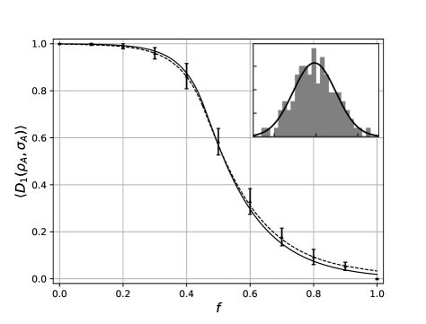
Figure 4: Subsystem trace-distances from exact diagoanlization for a chain of $10$ spins. Solid and dashed lines are the analytical predictions in absence and presence of conservation laws, Eqs. (8) and Eq. (11), respectively. Inset: Density of states for zero momentum eigenstates with Gaussian fit (solid line).

Appendix D Exact diagonaliztion

We numerically calculate eigenstates of the spin chain Hamiltonian first block diagonalizing $\hat{H}_{S}$ into momentum sectors, and then concentrating on eigenfunctions within the zero momentum eigenspace. To determine the energy window from which to choose eigenstates we calculate the density of states, see inset of Fig. 4 for the example of the chain with 10 spins. The latter is e.g. peaked at $-0.4\pm 0.3$ and reasonably well described by a Gaussian profile (solid line). Taking in this case $5$ eigenstates from the window $\sim(-0.8,0.0)$ centered around $\sim-0.4$ we arrive at the subsystem trace distance shown in Fig. 4, and compared to the analytical prediction in presence (dashed line) and absence (solid line) of a local conservation law.

References

- Page (1993) D. N. Page, Phys. Rev. Lett. 71, 1291 (1993), URL https://link.aps.org/doi/10.1103/PhysRevLett.71.1291.
- Bianchi and Donà (2019) E. Bianchi and P. Donà, Phys. Rev. D 100, 105010 (2019), URL https://link.aps.org/doi/10.1103/PhysRevD.100.105010.
- Bianchi et al. (2021) E. Bianchi, L. Hackl, M. Kieburg, M. Rigol, and L. Vidmar, Volume-law entanglement entropy of typical pure quantum states (2021), URL https://arxiv.org/abs/2112.06959.
- Rigol et al. (2008) M. Rigol, V. Dunjko, and M. Olshanii, Nature 452, 854 (2008), URL https://doi.org/10.1038/nature06838.
- Lau et al. (2022) P. H. C. Lau, T. Noumi, Y. Takii, and K. Tamaoka, Page curve and symmetries (2022), URL https://arxiv.org/abs/2206.09633.
- Ares et al. (2022) F. Ares, S. Murciano, and P. Calabrese, Journal of Statistical Mechanics: Theory and Experiment 2022, 063104 (2022), URL https://doi.org/10.1088.
- Vidmar and Rigol (2017) L. Vidmar and M. Rigol, Phys. Rev. Lett. 119, 220603 (2017), URL https://link.aps.org/doi/10.1103/PhysRevLett.119.220603.
- Nakagawa et al. (2018) Y. O. Nakagawa, M. Watanabe, H. Fujita, and S. Sugiura, Nature Communications 9, 1635 (2018).
- Sugiura and Shimizu (2012) S. Sugiura and A. Shimizu, Phys. Rev. Lett. 108, 240401 (2012), URL https://link.aps.org/doi/10.1103/PhysRevLett.108.240401.
- Sugiura and Shimizu (2013) S. Sugiura and A. Shimizu, Phys. Rev. Lett. 111, 010401 (2013), URL https://link.aps.org/doi/10.1103/PhysRevLett.111.010401.
- Murciano et al. (2022) S. Murciano, P. Calabrese, and L. Piroli, Phys. Rev. D 106, 046015 (2022), URL https://link.aps.org/doi/10.1103/PhysRevD.106.046015.
- Majidy et al. (2022) S. Majidy, A. Lasek, D. A. Huse, and N. Y. Halpern, Non-abelian symmetry can increase entanglement entropy (2022), URL https://arxiv.org/abs/2209.14303.
- Altland et al. (2022) A. Altland, D. A. Huse, and T. Micklitz, Maximum entropy quantum state distributions (2022), URL https://arxiv.org/abs/2203.12580.
- Bae and Kwek (2015) J. Bae and L.-C. Kwek, Journal of Physics A: Mathematical and Theoretical 48, 083001 (2015), URL https://doi.org/10.1088.
- foo (a) There are two kinds of errors i.e. the probability one guesses wrong when it is , and the probability one guess wrong when it is , respectively. The best success probability minimizes the maximum .
- foo (b) That is, the eigenvalues of , and when is hermitean, singular values are just the absolute values of the eigenvalues.
- Zhang et al. (2019) J. Zhang, P. Ruggiero, and P. Calabrese, Phys. Rev. Lett. 122, 141602 (2019), URL https://link.aps.org/doi/10.1103/PhysRevLett.122.141602.
- Monteiro et al. (2021) F. Monteiro, M. Tezuka, A. Altland, D. A. Huse, and T. Micklitz, Phys. Rev. Lett. 127, 030601 (2021), URL https://link.aps.org/doi/10.1103/PhysRevLett.127.030601.
- foo (c) Application of the replica trick allows for a calculation of the entanglement entropy from average moments of the reduced density matrix, , as .
- Penington et al. (2019) G. Penington, S. H. Shenker, D. Stanford, and Z. Yang, Replica wormholes and the black hole interior (2019), eprint arXiv:1911.11977.
- Liu and Vardhan (2020) H. Liu and S. Vardhan, Entanglement entropies of equilibrated pure states in quantum many-body systems and gravity (2020), eprint arXiv:2008.01089.
- Kreweras (1972) G. Kreweras, Discrete Mathematics 1, 333 (1972), ISSN 0012-365X, URL https://www.sciencedirect.com/science/article/pii/0012365X72900416.
- Simion (2000) R. Simion, Discrete Mathematics 217, 367 (2000), ISSN 0012-365X, URL https://www.sciencedirect.com/science/article/pii/S0012365X99002733.
- foo (d) The simplest way to see this, is to account for the sign factor in Eq. (4) by defining averages for states with a minus sign, i.e. . Then every cycle containing odd/even elements contributes with a negative/positive sign.
- Kudler-Flam et al. (2021) J. Kudler-Flam, V. Narovlansky, and S. Ryu, PRX Quantum 2, 040340 (2021), URL https://link.aps.org/doi/10.1103/PRXQuantum.2.040340.
- Puchała et al. (2016) Z. Puchała, Ł. Pawela, and K. Życzkowski, Phys. Rev. A 93, 062112 (2016), URL https://link.aps.org/doi/10.1103/PhysRevA.93.062112.
- foo (e) Notice that Eq. (11) diverges in the limits and , where and become -functions. In Fig. 2 we have interpolated with a quadratic polynomial to values from Eq. (C1) (Appendix C), with , and , , respectively, with an error of order .
- Sachdev and Ye (1993) S. Sachdev and J. Ye, Phys. Rev. Lett. 70, 3339 (1993), URL https://link.aps.org/doi/10.1103/PhysRevLett.70.3339.
- (29) A. Kitaev, http://online.kitp.ucsb.edu/online/ entangled15/kitaev/ …. /kitaev2/ (Talks at KITP on April 7th and May 27th 2015).
- Kim and Huse (2013) H. Kim and D. A. Huse, Phys. Rev. Lett. 111, 127205 (2013), URL https://link.aps.org/doi/10.1103/PhysRevLett.111.127205.
- Kim et al. (2014) H. Kim, T. N. Ikeda, and D. A. Huse, Phys. Rev. E 90, 052105 (2014), URL https://link.aps.org/doi/10.1103/PhysRevE.90.052105.
- Zhang et al. (2015) L. Zhang, H. Kim, and D. A. Huse, Phys. Rev. E 91, 062128 (2015), URL https://link.aps.org/doi/10.1103/PhysRevE.91.062128.
- foo (f) The SYK model preserves fermion parity and (without loss of generality) we have chosen eigenstates from the even parity sector.
- Srednicki (1994) M. Srednicki, Phys. Rev. E 50, 888 (1994), URL https://link.aps.org/doi/10.1103/PhysRevE.50.888.
- Kaufman et al. (2016) A. M. Kaufman, M. E. Tai, A. Lukin, M. Rispoli, R. Schittko, P. M. Preiss, and M. Greiner, Science 353, 794 (2016), URL https://www.science.org/doi/abs/10.1126/science.aaf6725.
- Dymarsky et al. (2018) A. Dymarsky, N. Lashkari, and H. Liu, Physical Review E 97 (2018), URL https://doi.org/10.1103/PhysRevE.97.012140.