THE LUMINOUS TYPE IIN SUPERNOVA SN 2017hcc: INFRARED BRIGHT, X-RAY AND RADIO FAINT

Abstract

We present multiwavelength observations of supernova (SN) 2017hcc with the Chandra X-ray telescope and the X-ray telescope onboard Swift (Swift-XRT) in X-ray bands, with the Spitzer and the TripleSpec spectrometer in near-infrared (IR) and mid-IR bands and with the Karl G. Jansky Very Large Array (VLA) for radio bands. The X-ray observations cover a period of 29 to 1310 days, with the first X-ray detection on day 727 with the Chandra. The SN was subsequently detected in the VLA radio bands from day 1000 onwards. While the radio data are sparse, synchrotron-self absorption is clearly ruled out as the radio absorption mechanism. The near- and the mid-IR observations showed that late time IR emission dominates the spectral energy distribution. The early properties of SN 2017hcc are consistent with shock breakout into a dense mass-loss region, with $\dot{M}\sim 0.1$ $M_{\odot}$ yr^-1 for a decade. At few 100 days, the mass-loss rate declined to $\sim 0.02$ $M_{\odot}$ yr^-1, as determined from the dominant IR luminosity. In addition, radio data also allowed us to calculate a mass-loss rate at around day 1000, which is two orders of magnitude smaller than the mass-loss rate estimates around the bolometric peak. These values indicate that the SN progenitor underwent an enhanced mass-loss event a decade before the explosion. The high ratio of IR to X-ray luminosity is not expected in simple models and is possible evidence for an asymmetric circumstellar region.

1 Introduction

The IIn class of supernovae (SNe IIn) was identified by Schlegel (1990) based on their narrow optical emission lines and hot continua. The narrow lines can be attributed to slow-moving circumstellar (CS) matter around the supernova (SN) and the luminosity can be identified with power provided by shock waves. If the cooling time for the gas is fast compared to the age, the SN power is efficiently converted to radiation in this class of supernovae (SNe). The required density of the circumstellar medium (CSM) is high in several SNe IIn (e.g. Fransson et al., 2014) and are generally not seen in Galactic sources outside of Luminous Blue Variables (LBVs) during outburst (Smith & Owocki, 2006; van Marle et al., 2008). Radioactivity is not a suitable power source for these SNe because it predicts a faster decline than observed.

In general, the first electromagnetic signal in SNe occurs when the shock reaches the SN photosphere and breaks out on time scales of minutes to hours. However, in dense winds shock breakout can happen in the CSM and last for an extended duration. There is increasing evidence that in some SNe IIn, the early light curves can be powered by shock breakouts (Chevalier & Irwin, 2011; Ofek et al., 2014; Waxman & Katz, 2017).

The early optical spectra of SNe IIn often show emission lines from a wind that are broadened by electron scattering (Chugai, 2001). Photons from the inner part of the mass-loss region scatter as they leave the mass-loss region. An electron column optical depth of about a few, or $10^{24}$ electrons cm^-2 column density, is needed to be consistent with the observations. At later times ($>100$ days), the line profiles are no longer consistent with electron scattering. Profiles are often fit by multiple Gaussians (e.g., Kiewe et al., 2012; Szalai et al., 2021). Although reasonable fits can be obtained, there is not a clear theory that points to Gaussian line shapes. Velocities corresponding to the line widths are larger than the thermal velocities in the optically emitting gas.

Considering the fast shock waves moving into a dense CSM, strong X-ray emission can be expected. Indeed, SNe IIn are well represented among the most X-ray luminous SNe (Dwarkadas & Gruszko, 2012; Chandra, 2018). However, there are optically luminous SNe IIn that are weak X-ray emitters; a prime example is SN 2006gy (Ofek et al., 2007; Smith et al., 2007). In some cases, the paucity of X-rays can be explained by the effects of high X-ray absorption due to the large column density through the CS matter (Chevalier & Irwin, 2012; Svirski et al., 2012). Low X-ray luminosity can also be attributed to a relatively low density CSM, as in the case of SN 1998S (Pooley et al., 2002). Chevalier & Irwin (2011) have shown that in some SNe high optical luminosity and low X-ray luminosity can be explained by shock breakout in dense surroundings.

SNe IIn can also be radio emitters from synchrotron radiation by shock accelerated electrons. Many high luminosity SNe IIn are also found to be weak emitters in radio bands (Chandra et al., 2015). While one expects a high intrinsic radio luminosity owing to a dense CSM, the same high density CSM could lead to efficient absorption of radio emission, e.g., the bright Type IIn SN 2010jl became radio bright only after 500 days (Chandra et al., 2015). Thus radio emission in SNe IIn is likely to be an interplay between the two. Internal free-free absorption can also play an important role in these SNe due to efficient mixing of cool gas between forward and reverse shock into the synchrotron emitting region (Weiler et al., 1990; Chandra et al., 2012; Chandra et al., 2020).

Gerardy et al. (2002) first described the late bright infrared (IR) emission from SNe IIn in which the IR light dominates the spectral energy distribution (SED). Such emission has been observed in many SNe IIn, including SN 1995N (Van Dyk, 2013), SN 1998S (Gerardy et al., 2000; Fassia et al., 2000; Mauerhan & Smith, 2012), SN 2006jd (Fox et al., 2011; Stritzinger et al., 2012), SN 2007rt (Trundle et al., 2009; Szalai et al., 2021), SN 2010jl (Fransson et al., 2014; Bevan et al., 2020), SN 2005ip (Fox et al., 2009, 2010; Stritzinger et al., 2012; Bak Nielsen et al., 2018), SN 2013L (Andrews et al., 2017) etc., beginning at an age of $\sim 1$ yr. The IR emission in these SNe has an approximately blackbody distribution, with a temperature $T$ in the range $\sim 700-1800$ K, which suggests that the emission is from dust.

There are two uncertainties about the dust emission: where is it located and how is it powered. Gerardy et al. (2002) and Fox et al. (2011) argue that the IR emission is from pre-existing dust that is beyond the evaporation radius and the forward shock front. In this case, a decline of the IR emission is expected once the forward shock has overrun the dust shell, around $3-4$ years after the explosion. Such a trend has been seen in some SNe IIn (Fox et al., 2011). On the other hand, efficient dust formation has been considered to be a viable scenario in interacting SNe, as the dust can form rapidly in the extremely dense, post-shock cooling layers (Smith, 2014). Gall et al. (2014) and Sarangi et al. (2018) propose that the dust in SN 2010jl formed in the cold dense shell (CDS) downstream from the radiative shock wave. They find that the dust can form at an age of about 1 year, when there is an increase in the IR emission from the SN. At earlier times, the radiation field is too strong to allow dust formation. In addition, dust may also form in the inner SN ejecta. Signatures of the dust formation were reported in SN 2006jc (Smith et al., 2008), SN 2005ip (Smith et al., 2009) and SN 2010bt (Elias-Rosa et al., 2018). The main signatures of dust formation are an IR excess, a drop in optical brightness via dust extinction, and asymmetry of the emission-line profiles due to dust attenuation (Smith, 2014).

While the most straightforward source for powering the late IR emission in SNe IIn would be continuing CS interaction, for SN 2010jl the evolution of the X-ray absorption column implies a drop in the CSM density at an age of about 1 year (Chandra et al., 2015; Sarangi et al., 2018; Dwek et al., 2021). The density drop would result in a drop in the power produced at the forward shock. To alleviate this Sarangi et al. (2018) suggested that the observed power is produced at the reverse shock wave, but the issue is unsettled.

SN 2017hcc (a.k.a ATLAS17lsn) was discovered on 2017 Oct. 2.38 UT (MJD 58028.38) by the Asteroid Terrestrial–impact Last Alert System (ATLAS, Tonry, 2011) and classified as Type IIn SN (Prieto et al., 2017). The SN reached a peak at 13.7 mag in around $40-45$ days, indicating an absolute peak magnitude of $-20.7$ mag at a distance $\sim 75$ Mpc (Prieto et al., 2017). The supernova was not detected on 2017 September 30.4 at a limiting magnitude of 19.04 mag, suggesting it was discovered soon after the explosion. We assume 2017 Oct 1 UT (MJD 58027) as the date of explosion throughout this paper.

Prieto et al. (2017) obtained a bolometric light curve by using a blackbody function to fit the SED using the data from ASAS-SN and the ultraviolet telescope (UVOT) onboard Swift. They obtained a peak luminosity of $L_{\rm bol,peak}=(1.34\pm 0.14)\times 10^{44}$ erg s^-1, making SN 2017hcc one of the most luminous SNe IIn ever (e.g., Smith et al., 2007; Ofek et al., 2014). They constrain the peak risetime to be $\sim 27$ days and the total radiated energy $\sim 4\times{10}^{50}$ erg. Early radio observations at 1.4 GHz with the Giant Metrewave Radio Telescope resulted in a non-detection (Nayana & Chandra, 2017).

A very high degree of intrinsic polarization at optical wavelengths was detected from SN 2017hcc  ($>4.8$%) (Mauerhan et al., 2017; Kumar et al., 2019). This is the strongest continuum polarization ever reported for a SN. Kumar et al. (2019) noted a 3.5% change in the Stokes V polarization in 2 months suggesting a substantial variation in the degree of asymmetry in either the ejecta and/or the surrounding medium of SN 2017hcc. They also estimated a mass-loss rate of $\dot{M}=0.12$ $M_{\odot}$ yr^-1  (for a wind speed of 20 km  s^-1), which is comparable to the mass-loss rate for an LBV in eruption. However, based on echelle spectra, Smith & Andrews (2020) suggested the CSM wind to be flowing axi-symmetrically with wind speeds of $v_{w}=40-50$ km s^-1 indicating bipolar geometry of the CSM created by losing 10 $M_{\odot}$ of stellar mass to eruptive mass ejections. Smith & Andrews (2020) modeled the optical and near IR emission of SN 2017hcc and found indications that the SN ejecta were hidden behind the photosphere until day 75. They found that the early time symmetric profiles changed to asymmetric blueshifted profiles at late times. They suggested the asymmetry to be time and wavelength dependent, causing a systematic blueshift in the line profiles. This was interpreted as a signature of the formation of new dust in the SN ejecta as well as in the post-shock gas within the CDS formed between the forward and the reverse shocks.

We carried out early to late time observations of SN 2017hcc with the Chandra and the X-ray telescope (XRT) onboard the Neil Gehrels Swift Observatory (Swift-XRT) telescopes in X-ray bands, with the Karl G. Jansky Very Large Array (VLA) in radio bands, and with Spitzer and the TripleSpec in IR bands. In this paper we report multiwaveband observations of SN 2017hcc and their interpretation. The observations are described in §2. Our main results are summarised in §3, and the discussion and comparison with published data are in §4. Finally, our main conclusions are summarised in §5.

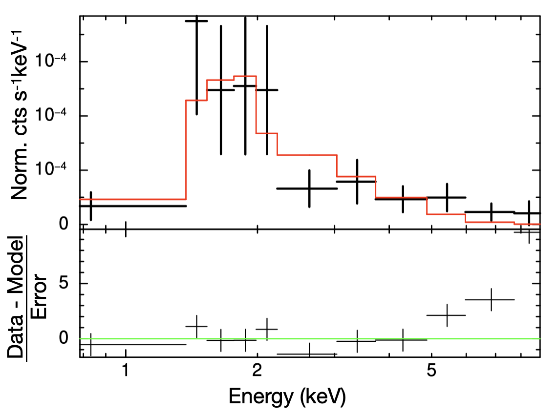
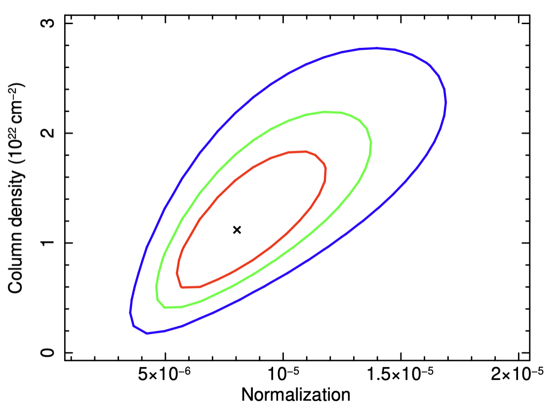
Figure 1: Left panel: Chandra ACIS-S spectrum of SN 2017hcc. The spectrum is fit with a thermal bremsstrahlung spectrum assuming a temperature of 3 keV. Right panel: Contours of best fit column density with the best fit normalization. The red, green and blue lines represent 1-$\sigma$, 2-$\sigma$ and 3-$\sigma$ contours.

2 Observations

2.1 Chandra Observations

We observed SN 2017hcc  with the Chandra ACIS-S on 2019 Sep 27 (MJD 58753) for an exposure of 40 ks. We extracted the spectrum, response and ancillary matrices using Chandra Interactive Analysis of Observations software (CIAO; Fruscione et al., 2006), using task specextractor. The CIAO version 4.6 along with CALDB version 4.5.9 was used for this purpose. The HEAsoft package Xspec version 12.1 (Arnaud, 1996) was used to carry out the spectral analysis. Due to low counts, only 5 channels were averaged and we used maximum likelihood statistics for a Poisson distribution, i.e. the $c$-statistics (Cash, 1979).

The spectrum was fit with an absorbed thermal bremsstrahlung model. In the view of Smith & Andrews (2020), the optical measurements implied a SN ejecta velocity of 4000 km s^-1  around the Chandra epoch and a CDS velocity of 1600 km s^-1 . Assuming the CDS velocity to be that of the forward shock, the reverse shock velocity is 2400 km s^-1   (Smith & Andrews, 2020). However, in SNe IIn the CDS generally absorbs any X-ray emission coming from the reverse shock due to the high column density of cool gas, and the dominant emission is likely to come from the forward shock (Margutti et al., 2014; Ofek et al., 2014; Chandra et al., 2015). The forward shock velocity of 1600 km s^-1  estimated by Smith & Andrews (2020) corresponds to a temperature of $\sim 3$ keV, which is what we initially assume to fit the Chandra spectrum. Our observation resulted in a detection with an unabsorbed $0.3-10$ keV luminosity of $1.94\times 10^{40}$ erg s^-1 . The best fit column density is $1.13^{+0.78}_{-0.58}\times 10^{22}$ cm^-2  (Fig. 1).

We, however, note that the forward shock velocity could be larger than the above value, as discussed in §4.1. To reflect this possibility, we also ran the fits by fixing the X-ray emitting shocked plasma temperature to be 20 keV (corresponding to a forward shock velocity of 4000 km s^-1 , an estimate based on observations of SN 2010jl at an age of 737 days (Ofek et al., 2014; Chandra et al., 2015)). In this case, our observation resulted in an unabsorbed $0.3-10$ keV luminosity of $1.74\times 10^{40}$ erg s^-1 . The best fit column density is $(5.7^{+6.2}_{-4.5})\times 10^{21}$ cm^-2 . While the X-ray luminosity is lower by only 10% for 20 keV plasma as compared to that with 3 keV plasma, the best fit column density is lower by a factor of 2, though we note that the uncertainty in column density is large with a 3-$\sigma$ upper limit of $\sim 2\times 10^{22}$ cm^-2 . Hence this is roughly consistent with the previous value.

2.2 Swift-XRT Observations

We observed SN 2017hcc with the Swift-XRT starting 2017 Oct 28 (MJD 58054). The observations continued until 2021 May 03 (MJD 59337) at various epochs. The measurements were taken in the photon counting mode. The xselect program of the HEAsoft package (version 6.28, CALDB version (XRT(20210915))) was used to create the spectra and images. Observations closely spaced in time were combined. None of the Swift-XRT observations resulted in detection with 3-$\sigma$ upper limits ranging around $\sim(1-4)\times 10^{-3}$ counts s^-1. The $0.3-10.0$ keV flux was obtained from the $3\sigma$ upper limits on the count rates by assuming a thermal plasma of 3 keV and a column density of $1.1\times 10^{22}$ cm^-2 . The details are given in Table 1.

Table 1: X-ray observations of SN 2017hcc

Date of	MJD	Telescope	Exposure	Age	Count rate	Unabs. Flux	Unabs. Luminosity
Observation (UT)			(ks)	(day)	(cts s-1)	(erg s-1 cm-2)	(erg s-1)
$\sim$ 2017 Oct 30	58056	Swift-XRT	13.47	29	$<1.02\times 10^{-3}$	$<0.54\times 10^{-13}$	$<3.64\times 10^{40}$
$\sim$ 2017 Nov 17	58074	Swift-XRT	5.20	47	$<2.56\times 10^{-3}$	$<1.35\times 10^{-13}$	$<8.97\times 10^{40}$
$\sim$ 2017 Dec 10	58097	Swift-XRT	9.58	70	$<1.03\times 10^{-3}$	$<0.55\times 10^{-13}$	$<3.65\times 10^{40}$
2018 May 23	58261	Swift-XRT	4.94	235	$<3.85\times 10^{-3}$	$<2.05\times 10^{-13}$	$<13.7\times 10^{40}$
2019 Sep 27	58753	Chandra ACIS-S	40.53	727	$(1.28\pm 0.36)\times 10^{-3}$	$(2.87\pm 0.53)\times 10^{-14}$	$(1.94\pm 0.43)\times 10^{40}$
2021 May 03	59337	Swift-XRT	4.71	1310	$<2.81\times 10^{-3}$	$<1.48\times 10^{-13}$	$<10.0\times 10^{40}$

For Chandra observations, the temperature was fixed to 3 keV (see §4). The best fit column density is $N_{H}=(1.13^{+0.78}_{-0.58})\times 10^{22}$ cm^-1. The count rates have been converted to fluxes assuming a thermal plasma of 3 keV and column density of $1.1\times 10^{22}$ cm^-1 for the Swift-XRT observations.

2.3 Spitzer observations

SN 2017hcc  was observed with the Infrared Array Camera (IRAC) (Fazio et al., 2004) onboard Spitzer (Werner et al., 2004) at three epochs (PI: Fox), starting 2018 Oct 29 (MJD 58420; Table 2). We used the Spitzer Heritage Archive (SHA) to download Post Basic Calibrated Data (pbcd), which are already fully coadded and calibrated. Standard aperture photometry was performed, although separate apertures were strategically placed by eye to best estimate the local background. Figure 2 plots and Table 2 lists the mid-IR photometric data, which are also included in a comprehensive Spitzer paper by Szalai et al. (2021).

As in the analysis laid out by Fox et al. (2011), the mid-IR photometry can be fit as a function of the dust temperature, $T_{d}$, and mass, $M_{d}$. Given only two photometry points per epoch, we assume a simple blackbody model, consisting of a single graphite grain of size 1 $\mu$m and a single temperature. We calculate opacities using the optical constants from Draine & Lee (1984).Table 2 lists the results and Figure 2 shows the Spitzer data.

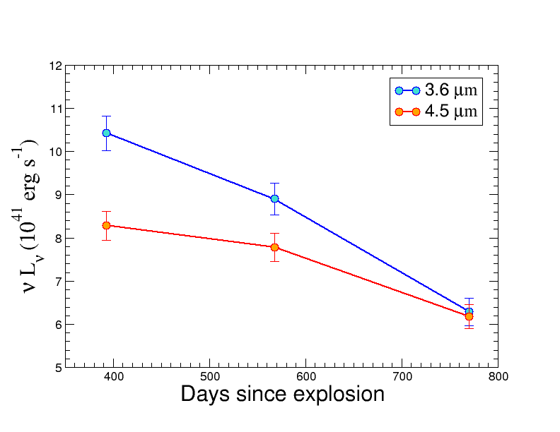
Figure 2: Spitzer photometry of SN 2017hcc. The data are taken at 3 epochs (2018 Oct 29 (day 393), 2019 Apr 21 (day 568) and 2019 Nov 9 (day 770)) at 3.6 and 4.5 $\mu$m wavelengths (§2.3). The temporal evolution indices at 3.6$\mu$m between days 393 and 568, and days 568 and 770 are $-0.43\pm 0.15$, and $-1.14\pm 0.22$, respectively. The temporal evolution indices at 4.5$\mu$m between days 393 and 568, and days 568 and 770 are $-0.17\pm 0.16$, and $-0.76\pm 0.20$, respectively.

Table 2: Spitzer IRAC observations of SN 2017hcc

Quantity	Wavelength	Date of observations
		2018 Oct 29.35	2019 Apr 20.58	2019 Nov 08.57
		(MJD 58420.35)	(MJD 58593.58)	(MJD 58795.57)
AOR id		66120960	68799232	68799488
Epoch (d)		393	568	770
Apparent magnitude	3.6$\mu$m	12.97$\pm$0.04	13.16$\pm$0.05	13.52$\pm$0.05
	4.5$\mu$m	12.49$\pm$0.04	12.56$\pm$0.04	12.81$\pm$0.04
Absolute magnitude	3.6$\mu$m	-21.32$\pm$0.19	-21.14$\pm$0.19	-20.77$\pm$0.19
	4.5$\mu$m	-21.80$\pm$0.19	-21.73$\pm$0.19	-21.48$\pm$0.19
Flux density ($\mu$Jy)	3.6$\mu$m	$1818.72\pm 70.35$	$1533.79\pm 64.98$	$1097.13\pm 55.58$
	4.5$\mu$m	$1813.78\pm 71.83$	$1703.51\pm 69.03$	$1354.05\pm 62.36$
$\nu L_{\nu}$ (erg s-1)	3.6$\mu$m	$(10.42\pm 0.40)\times 10^{41}$	$(8.90\pm 0.37)\times 10^{41}$	$(6.29\pm 0.32)\times 10^{41}$
	4.5$\mu$m	$(8.28\pm 0.33)\times 10^{41}$	$(7.78\pm 0.32)\times 10^{41}$	$(6.18\pm 0.28)\times 10^{41}$
Dust massa ($M_{\odot}$)		$2.26\times 10^{-3}$	$3.60\times 10^{-3}$	$4.57\times 10^{-3}$
Dust Temp (K)		$1.28\times 10^{3}$	$1..07\times 10^{3}$	$0.93\times 10^{3}$
$L_{\rm bol}$b (erg s-1)		$4.80\times 10^{41}$	$3.73\times 10^{41}$	$2.70\times 10^{41}$
Blackbody radius (cm)		$1.57\times 10^{16}$	$1.97\times 10^{16}$	$2.23\times 10^{16}$

^a The dust mass estimates are sensitive to the chosen grain parameters. The listed values are estimated assuming 1 $\mu$m grain size of graphite composition.

^b Bolometric luminosity assuming a single temperature dust blackbody radiation.

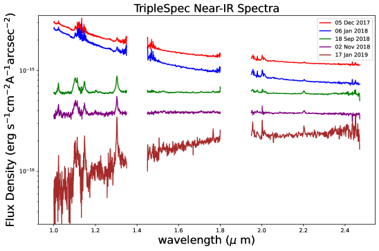
Figure 3: Triplespec near-IR spectra of SN 2017hcc on 2017 Dec 05 (day 66), 2018 Jan 06 (day 98), 2018 Sep 18 (day 353), 2018 Nov 02 (day 398) and 2019 Jan 17 (day 474). Note that the early spectra are brighter at lower wavelengths, whereas the late time spectra are brighter at longer wavelengths. To show this trend better, the top four spectra are offset by $10^{-15}$, $6\times 10^{-16}$, $5\times 10^{-16}$, and $3\times 10^{-16}$ erg s^-1 cm^-2 A^-1 arcsec^-2, respectively.

2.4 TripleSpec Observations

We obtained five epochs, 2017 Dec 05 (MJD 58092), 2018 Jan 6 (MJD 58124), Sep 18 (MJD 58379), Nov 02 (MJD 58424) and 2019 Jan 17 (MJD 58500), of near-IR spectroscopy, with simultaneous continuous wavelength coverage from 0.95-2.46 $\mu$m in five spectral orders, with the TripleSpec spectrograph at the Apache Point Observatory 3.5-m (Wilson et al., 2004). Our observation sequence consists of 300-s dithered exposures that could be pair subtracted to allow for correction of thermal background and night-sky emission lines. We used a modified version of SpexTool for the spectral extraction (Cushing, 2004). While the early data are dominated by shorter wavelength emission, the later data reveal higher flux densities at longer wavelengths (Fig. 3). However, we note a caveat here that due to calibration uncertainty the TripleSpec flux should not be considered absolute and ideally should be scaled to near-IR photometry.

2.5 VLA observations

The VLA observed SN 2017hcc between 2020 June 29–30 (MJD 59029–59030) in bands X (8–12 GHz) and K (18–26 GHz), and later in June 2021 in Ka (26–40 GHz), Ku (12–18  GHz), X, C (4–8 GHz) and S (2–4 GHz) bands. The data were analysed using the standard packages within the Common Astronomy Software Applications package (CASA, McMullin et al., 2007). The details of the observations and the flux density values can be found in Table 3. We add 10% error in the quadrature to the flux density values for analysis purposes, a typical uncertainty in the flux density calibration scale at the observed frequencies .

Table 3: Radio observations of SN 2017hcc

Date of	MJD	Telescope	Age	Central	Flux density	rms	Luminosity	$\nu L_{\nu}$
Obs. (UT)			(days)	Freq (GHz)	$\mu$Jy	$\mu$Jy	(erg s-1 Hz-1)	(erg s-1)
2020 Jun 29	59029	VLA	1002	10.0	32.5$\pm$7.6	6.7	$(2.19\pm 0.51)\times 10^{26}$	$(2.19\pm 0.51)\times 10^{36}$
2020 Jun 30	59030	VLA	1003	22.0	77.1$\pm$16.2	15.5	$(5.19\pm 1.09)\times 10^{26}$	$(11.42\pm 2.40)\times 10^{36}$
2021 Jun 04	59369	VLA	1342	10.0	$<45.6$	15.26	$<3.07\times 10^{26}$	$<3.07\times 10^{36}$
2021 Jun 09	59374	VLA	1347	15.4	31.0$\pm$11.3	10.5	$(2.09\pm 0.76)\times 10^{26}$	$(3.21\pm 1.17)\times 10^{36}$
2021 Jun 09	59374	VLA	1347	6.1	$<26.7$	8.9	$<1.80\times 10^{26}$	$<1.10\times 10^{36}$
2021 Jun 11	59376	VLA	1349	3.0	$<182.4$	60.7	$<12.28\times 10^{26}$	$<3.68\times 10^{36}$
2021 Jun 14	59379	VLA	1352	33.1	33.5$\pm$11.8	11.6	$(2.26\pm 0.79)\times 10^{26}$	$(7.46\pm 2.63)\times 10^{36}$
2021 Jun 16	59381	VLA	1354	1.5	$<228$	76.1	$<15.34\times 10^{26}$	$<2.30\times 10^{36}$

3 Analysis and Results

3.1 X-ray analysis and the column density

Swift-XRT observations of SN 2017hcc started when the SN was around a month old; however, the first X-ray detection of SN 2017hcc was at an age of $\sim 2$ years with the Chandra telescope. Our Chandra observations did not have enough counts to determine the shock temperature and the column density separately. We assumed a temperature of $\sim 3$ keV, corresponding to a CDS velocity of 1600 km s^-1 , as advocated by Smith & Andrews (2020). The best fit column density is $1.13^{+0.78}_{-0.58}\times 10^{22}$ cm^-2  (Fig. 1). The Milky Way line of sight reddening is $E(B-V)=0.0285$ and that through the host galaxy is $E(B-V)=0.016$ (Smith & Andrews, 2020). These values correspond to their respective column densities of $N_{H,\rm MW}=1.64\times 10^{20}$ cm^-2  and $N_{H,\rm host}=0.92\times 10^{20}$ cm^-2 , using Schlafly & Finkbeiner (2011) recalibration of the Schlegel et al. (1998) extinction map. To derive $N_{H}$ we use $N_{H}=E(B-V)\times 5.8\times 10^{21}$ cm^-2 . However, this relation is an empirical relation and has uncertainties (e.g. Gudennavar et al., 2012; Liszt, 2019). Combining the column density due to the Milky Way and the host galaxy gives $2.56\times 10^{20}$ cm^-2 , which has negligible effect on the best fit column density which is two orders of magnitude higher. The excess column density comes from the CSM, i.e. $N_{H,\rm CSM}=\sim 1.10\times 10^{22}$ cm^-2 .

The $0.3-10.0$ keV unabsorbed flux is $f_{0.3-10\,\rm keV}=(2.87\pm 0.53)\times 10^{-14}$ erg cm^-2 s^-1, corresponding to a luminosity of $L_{0.3-10\,\rm keV}=(1.94\pm 0.43)\times 10^{40}$ erg s^-1. This value does not change significantly even if we use an X-ray emitting plasma temperature of 20 keV based on the temperature observed in SN 2010jl (Ofek et al., 2014; Chandra et al., 2015). In Fig. 4, we plot the SN 2017hcc X-ray luminosity along with other well-observed SNe IIn. Other than SN 1978K and SN 1998S, detected SNe IIn are brighter than SN 2017hcc. The SN 2017hcc luminosity is comparable to that of SN 1998S at the same age. We discuss the possible reasons for low X-ray luminosity in §4.

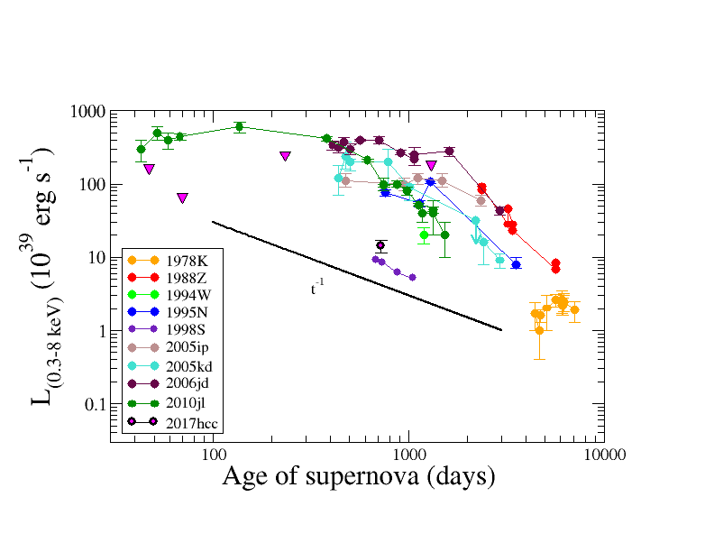
Figure 4: The 0.3–8 keV luminosities of X-ray detected SNe IIn. The Chandra SN 2017hcc detection is marked with a big magenta circle and the Swift upper limits with inverted triangles. Reproduced from Chandra (2018).

3.2 IR analysis

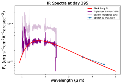
Figure 5: The spectra on day $\sim 395$ combined with TripleSpec and Spitzer data. The light purple color shows original spectrum, whereas the purple spectrum has been shifted upwards to match the blackbody curve passing through the 3.6 $\mu$m Spitzer  data point.

SN 2017hcc is extremely bright at Spitzer IRAC wavelengths. The 4.6 $\mu$m absolute magnitude reached $-21.7$ mag after a year, which corresponds to a peak IR luminosity $\sim 10^{42}$ erg s^-1. The late time emission is dominated by the IR emission (Smith & Andrews, 2020), as is frequently the case for SNe IIn (see §1). We estimate the temporal evolution $\beta$ (where $\beta$ is defined as $F_{\nu}(t)\propto t^{\beta}$) and between Spitzer flux densities ($F_{\nu}(t)$) in $\mu$Jy (Fig. 2). The temporal evolution between epochs 1 and 2, at 3.6 and 4.5 $\mu$m, are $\beta=-0.46\pm 0.16$ and $\beta=-0.17\pm 0.15$, respectively. The temporal indicies between the epochs 2 and 3 at the two frequencies are $\beta=-1.10\pm 0.21$ and $\beta=-0.76\pm 0.20$. The spectral indices $\alpha$ (defined as $F_{\nu}\propto\nu^{\alpha}$) between the two wavelengths at each epoch are $\alpha=-0.01\pm 0.25$, $\alpha=0.47\pm 0.26$ and $\alpha=0.94\pm 0.31$, respectively. The slow decline of the IR emission, combined with the fast optical decline (Kumar et al., 2019; Smith & Andrews, 2020), has important implications for the origin of the dust (§4.5).

The TripleSpec data at five epochs: 2017 Dec 5 (d 65), 2018 Jan 6 (d 97), Sep 18 (d 352), Nov 02 (d 397) and 2019 Jan 17 (d 473) are plotted in Fig. 3. While the early data are dominated by shorter wavelength emission, the later data reveal higher flux densities at longer wavelengths. A growing IR excess over the photospheric emission develops over time. We combine the measurements of Spitzer and TripleSpec on 2018 Oct 29 and 2018 Nov 2, respectively, and fit a simple blackbody model to the combined spectrum. The IR spectra using these data are plotted in Fig. 5. However, the calibration of the TripleSpec data has large uncertainties and hence the flux should not be considered absolute. Ideally it should be scaled to near-IR photometry. We have varied the scaling of the TripleSpec spectrum manually, and tried to shift to the blackbody curve passing through the Spitzer 3.6 $\mu$m data point. While the blackbody curve with $T\approx 1600$ K fits the data reasonably well, there seems to be a slight excess of the 4.5 $\mu$m flux. However, the significance of the fit is low due to the calibration uncertainties and the fact that the scaled TripleSpec spectrum does not seem to go through both the Spitzer data points and thats causes the uncertainty in the scaling factor. Hence we do not use the parameters derived from these fits.

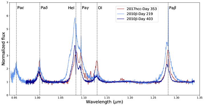
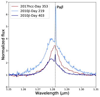
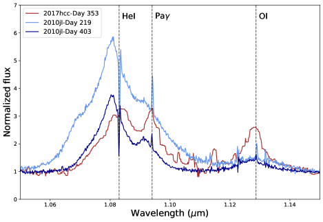
Figure 6: Comparison of near IR spectra of SN 2017hcc (Borish et al., 2015) with those of SN 2010jl. Spectra are normalized to the continuum level. The SN 2017hcc spectrum is on day 353 (brown lines, corresponding to Triplesec data on 2018 Sep 18 (MJD 58379)). SN 2010jn spectra are on day 219 (light blue lines) and day 403 (dark blue lines) Top panel: The full spectra. Bottom two panels show zoomed plots for O I, Pa $\beta$, Paschen $\gamma$ and He I lines.

We compare the SN 2017hcc near IR TripleSpec spectra with those of SN 2010jl in Figure 6. The two SNe have qualitatively similar characteristics but there are significant differences. In SN 2017hcc, the O I (1.129 $\mu$m) line is much stronger relative to Pa$\beta$ (1.282 $\mu$m) than in SN 20201jl, while the He I (1.083 $\mu$m) line is weaker relative to Pa$\beta$. The H lines show some asymmetry towards the blue side in SN 2017hcc, This is seen visually as a greater area under the lines to the blue side of the central wavelength vs the red side. But the asymmetry is less than that in SN 2010jl. This could be due to dust formation in the post-shock shell and in the SN ejecta, which progressively obscures the redshifted part. Any associated CS dust was presumably evaporated by the SN. Narrow lines like those observed in SN 2010jl are present in SN 2017hcc  (Smith & Andrews, 2020), but are not resolved here. The width of the expected narrow lines is $\sim 50$ km s^-1 , whereas the TripleSpec resolution is $\sim 100$ km s^-1 . The estimated wind velocity is 100 km s^-1 for SN 2010jl (Fransson et al., 2014), but is $40-50$ km s^-1 for SN 2017hcc (Smith & Andrews, 2020)

3.3 Radio Analysis

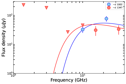
Figure 7: Radio spectra of SN 2017hcc with the VLA at two epochs. The spectra on day 1000 is in blue color and the one on day 1347 is in red color. The triangles represent upper limits. A simple FFA model is fit to the data.

The VLA measurements show faint detections ($\leq 5\,\sigma$, as mentioned in Table 3 and Fig. 7). The peak spectral luminosity is $5.2\times 10^{26}$ erg s^-1 Hz^-1, which is towards the lower end of the SNe IIn luminosities (Chandra, 2018). The day 1000 spectral index between these frequencies is $+1.1$. This indicates that the supernova is still moderately optically thick. Such behavior has been observed in the early evolution of other SNe IIn such as SN 1986J which showed $\alpha\sim+1.5$ in its rise to maximum (Weiler et al., 1990) and has been attributed to clumpiness in the emitting region (Weiler et al., 1990). Our radio data taken a year later show a higher radio luminosity. The spectral indices between the detected points are flat, indicating that the radio emission is near its transition from optically thick to thin regime. Due to the small number of data points, we fit the simple free-free absorption (FFA) model used in Chandra et al. (2012) assuming an optically thin spectral index of $-0.6$. The best fits at the two epochs are shown in Fig. 7. We also attempt to fit the synchrotron self-absorption model (SSA) and from the peak we estimate the SSA velocity using the formulation in Chevalier (1998). This velocity is around $\sim 150$ km s^-1 , which is an order of magnitude smaller than the ejecta velocity. This rules out SSA as a significant absorption mechanism.

4 Discussion

4.1 Shock breakout in presupernova mass-loss

With a peak bolometric luminosity of $1.3\times 10^{44}$ erg s^-1 reached in $\sim 30$ days and an absolute magnitude of $-20.7$ mag (Prieto et al., 2017), SN 2017hcc is at the boundary of superluminous supernovae with a two orders of magnitude larger luminosity than normal core-collapse supernovae. In addition, strong narrow lines are present (Smith & Andrews, 2020), indicating that dense outflowing circumstellar gas surrounds the supernova. If this gas is sufficiently optically thick, the shock breakout radiation from the supernova will occur after the interaction shell has moved to the mass-loss region. Quantitatively, if the wind optical depth is $\tau_{\rm w}$ and $v_{\rm sh}$ is the shock speed, then for cases where $\tau_{\rm w}>c/v_{\rm sh}$, the SN shock breaks out in the wind. Such a breakout through the thick wind may extend long enough, lasting days to months, and may account for the peak SN luminosity of SN 2017hcc  (Chevalier & Irwin, 2011).

We use the approximate formulation of Chevalier & Irwin (2011) for shock breakout in a wind. An initial assumption for this is that the mass-loss density profile is that for a steady wind, $\rho=Dr^{-2}$, where $D=\dot{M}/(4\pi R^{2}v_{\rm w})$. As per their formulation, there are two length scales that are important. One, $R_{\rm d}$, is the radius at which the diffusion time equals the expansion time, so photons can move out through the wind. We have $R_{\rm d}=\kappa Dv_{\rm sh}/c$, where $\kappa$ is the opacity. The other important length scale is $R_{\rm w}$ where the wind density cuts off. The character of the shock breakout is expected to depend on whether $R_{\rm w}>R_{\rm d}$, when the diffusion is important, or vice versa for which the diffusion time scales are large (Chevalier & Irwin, 2011). The indications are that SN 2017hcc is in the case $R_{\rm w}>R_{\rm d}$. This is indicated by the presence of bright infrared emission to late times (2 years) implying that the mass loss region extends to large radius. Also, the narrow line emission in optical bands (Smith & Andrews, 2020) shows a dense mass loss region. We scale the parameter $D$ to $D_{*}$ such that $D_{*}=D/(5\times 10^{16}$ g cm^-1) corresponding to a mass loss rate of $0.1M_{\odot}$ yr^-1 and wind velocity of 100 km s^-1. Here $D$ is in g cm^-1 and $D_{*}$ is a dimensionless quantity. As mentioned earlier, in SN 2017hcc the rise time can be approximated by the rise time of the bolometric light curve, 30 days (Prieto et al., 2017), so $D_{*}\approx 4.5$. For the wind velocity of 45 km s^-1, we get $\dot{M}=0.1M_{\odot}$ yr^-1 which should apply near the time of maximum light.

At shock breakout, a radiation dominated shock can no longer be maintained and a cold dense shell (CDS) forms at the shock interface. A simple model for a supernova density profile, used by Chevalier & Irwin (2011), is an inner region with a flat density surrounded by a steep $\rho\propto r^{-7}$ profile. For typical parameters, the interaction region between the ejecta and the CSM is in the steep power law region. For normal supernova parameters, Equation (6) in Chevalier & Irwin (2011) shows that the breakout luminosity can be close to that observed in SN 2017hcc near bolometric peak.

In the above we use 4000 km s^-1 for the shock velocity, as indicated in the X-ray observations of SN 2010jl (Chandra et al., 2015) and SN 2014C (Margutti et al., 2017). Here we discuss the shock velocity. Smith & Andrews (2020) determine $v_{\rm sh}$ from the emission line profiles of H$\alpha$ and H$\beta$. They find that the line profiles can be fit by 2 Gaussian components, one with a FWHM of 4000 km s^-1 and one with 1100 km s^-1, which they identify with emission from the freely expanding ejecta and the CDS, respectively. After allowance for a geometrical factor, Smith & Andrews (2020) use 1600 km s^-1 for $v_{\rm CDS}$, where $v_{\rm CDS}=v_{\rm sh}$ for a thin shell. However, there is no clear physical reason for the emission from the CDS or ejecta to have a Gaussian profile with a width corresponding to a physical parameter. Dessart et al. (2015) modeled the emission from SN 2010jl and found reasonable estimates for the line profile of H$\alpha$ considering emission from the CDS with electron scattering and CDS velocity $\sim 3000$ km s^-1. Also, in a spherically symmetric interaction, a large, unexpected deceleration would be required between the ejecta and the CDS for the values mentioned by Smith & Andrews (2020). In the formation of a thin shell between ejecta with power law index $n$ and CSM with power law $s$, we have $R\propto t^{(n-3)/(n-s)}$ (Chevalier, 1982) so that $v_{\rm ej}/v_{\rm CDS}=(n-s)/(n-3)$. For typical values $n=8$ and $s=2$ (e.g., Fransson et al., 2014, for SN 2010jl), we have $v_{\rm ej}/v_{\rm CDS}=1.2$, as opposed to $v_{\rm ej}/v_{\rm CDS}=2.50$ from the line observations (Smith & Andrews, 2020). The low value of $v_{\rm CDS}$ is not consistent with the type of evolution seen in SN 2010jl during the first year if there is spherically symmetric expansion. Other estimates for $v_{\rm CDS}$ can be considered. In the case of SN 2010jl, an X-ray observation at 2 yr with NuSTAR showed a temperature of 20 keV (Ofek et al., 2014; Chandra et al., 2015), which corresponds to a shock velocity of 4,000 km s^-1. A higher velocity would be expected at earlier times and there is possible evidence for a higher velocity from a feature that appears in the He I line in SN 2010jl (Borish et al., 2015; Chandra et al., 2015). We consider both small and large values for $v_{\rm CDS}$.

For the shock front to break out in the wind region, $\tau_{\rm w}>c/v_{\rm sh}$ is needed. Taking $R_{\rm b}$ to be the radius of the base of the wind, we have $\tau_{w}\approx 5\times 10^{16}kR_{\rm b}^{-1}D_{*}$, where $k$ is the opacity $\kappa$ in units of 0.34 cm²g^-1 (Chevalier & Irwin, 2011). As discussed above, for $D_{*}=4.5$, this gives $\tau_{w}\approx 76(R_{\rm b}/{10^{15}{\rm cm}})^{-1}$. Thus for reasonable parameters, the shock breakout does occur in the wind.

One aspect of shock breakout is that the temperature should increase with rising luminosity, since the initial rise to maximum luminosity should be primarily due to heating of the photosphere. This has not been seen in SN 2017hcc (Kumar et al., 2019). However, we note that the early measurements for temperature are not available before the peak in the light curve.

4.2 Post-Breakout Interaction

Once the diffusion time is less than the supernova age, the luminosity corresponds to the power generated at the shock. We have a luminosity $L=4\pi R^{2}\epsilon\frac{1}{2}\rho v_{\rm sh}^{3}$, where $R$ is the radius of the CDS and $\epsilon$ is an efficiency factor for the conversion of shock power to radiation (Chugai, 1990). At early times, the cooling time is less than the age so the shock power is radiated and $\epsilon\approx 1$. With sufficient good quality data, the winds of SNe IIn are generally found to be not steady (Dwarkadas, 2007), but the assumption should lead to a rough estimate for $\dot{M}$, which, for a steady wind is:

$$\dot{M}=2Lv_{\rm w}/\epsilon v_{\rm sh}^{3}$$ (1)

The value of $v_{\rm w}$ can be estimated from high spectral resolution observations. Smith & Andrews (2020) find $v_{\rm w}\approx(40-50)$ km s^-1. To estimate the value of $\dot{M}$, we use the bolometric luminosity of $\sim 10^{42}$ erg s^-1 which is the luminosity of infrared dust emission at $1-2$ yr (Table 2). We now find from Equation 1 $\dot{M}=2\times 10^{-3}\epsilon^{-1}L_{42}(v_{\rm sh}$/ 4000 km s${}^{-1})^{-3}$ $M_{\odot}$ yr^-1, where $v_{w}=45$ km s^-1 is assumed, and $L_{42}$ is the bolometric luminosity in the units of $10^{42}$ erg s^-1. So we now have $D_{*}\approx 0.024$. We note that the value of $v_{\rm w}$ is determined over the first 100 days (Smith & Andrews, 2020); there could be a change at later times. In addition, the value of the mass loss is sensitive to the shock velocity. However, our results indicate that the mass loss density drops more rapidly with radius than in the steady ($r^{-2}$) case.

The cooling of the postshock gas is important for the value of $\epsilon$ in the above formula. We now discuss the validity of cooling. Our discussion is similar to that of Chevalier & Fransson (2017). For electron temperature $T_{\rm e}\gtrsim 2.6\times 10^{7}$ K, which is expected for the post-forward shock wave, free-free cooling dominates with a cooling rate $\Lambda=1.0\times 10^{-23}(T_{e}/10^{7}\,{\rm K})^{0.5}$ erg s^-1 cm³. Assuming isobaric cooling behind the shock, the cooling time is $t_{\rm cool}=5kT_{e}/n_{H}\Lambda(T_{e})$. Using Chevalier & Fransson (2017) eqn. (18), the transition time at which the age equals the cooling time, for ejecta velocity 4000 km s^-1 (indicated with $v_{\rm ej,4}$ in the formula below) is (for $n=8$)

$$t_{\rm tr}=342D_{*}v_{\rm ej,4}^{-3}{\rm days}.$$ (2)

which is 75 days for our preferred parameters. This estimate would imply that the supernova was past the cooling phase at the time of the X-ray observation. However, the uncertainties are large so some effect of cooling cannot be ruled out. The estimates should be taken with caution, since the properties of the absorbing gas are uncertain because of early Compton heating and radiative cooling as well as recombination (Lundqvist & Fransson, 1988).

4.3 Variable mass-loss rate

The above treatment shows that the mass-loss rate obtained at $\sim 30$ days from the shock breakout was $\sim 0.1$ $M_{\odot}$ yr^-1, whereas at few hundred days, obtained from the IR measurements, was $\sim 2\times 10^{-3}$ $M_{\odot}$ yr^-1. In addition, we can also use the timing of the peak radio flux density to estimate the mass-loss rate at $\sim 1000$ d. The mass-loss rate derived from our radio measurement assuming a CSM temperature of $10^{4}$ K is $\sim 6.5\times 10^{-4}$ $M_{\odot}$ yr^-1. These epochs correspond to roughly $\sim 10$, $\sim$100 and $\sim$300 days before explosion and the mass loss rate changes roughly two to three orders of magnitude. This indicates a variable mass-loss rate, with enhanced mass-loss event occurring a decade before the supernova explosion.

There is growing number of evidence that many core-collapse supernovae undergo similar enhancements during the last years before the explosion. Maeda et al. (2021) reported evidence of enhanced mass-loss in nearby type Ic supernova SN 2020oi in their Atacama Large Millimeter Array (ALMA) observations, which they interpreted as the pre-SN activity likely driven by the nuclear burning activities in the star’s final moments. Similar conclusions were drawn for the famous supernova SN 2014C undergoing metamorphosis from a stripped envelope supernova to a Type IIn via their radio and X-ray observations (Anderson et al., 2017; Margutti et al., 2017; Brethauer et al., 2022). The flash spectroscopy of various supernovae have also revealed the similar conclusions. A remarkable example is SN 2013fs, discovered mere 3 hrs after the explosion by the automated real-time discovery and classification pipeline of the intermediate Palomar Transient Factory (iPTF) survey, which enabled spectroscopy measurements within 6 hours of discovery (Yaron et al., 2017). The early measurements revealed a dense CSM to be confined within $10^{15}$ cm indicating enhanced mass-loss ($10^{-3}$ $M_{\odot}$ yr^-1) in the last one year before explosion in an otherwise normal core-collpase supernova. This led authors to suggest that such pre-SN activities may be common in exploding stars. Shivvers et al. (2015) examined the Keck HIRES spectrum of SN 1998S taken within a few days after the SN and found convincing evidence for enhanced mass-loss rate in the last 15 years of star’s life. These measurements combined with other published measurements indicated much smaller mass-loss rate at earlier times, arriving at the conclusion of this section. SN 2020tlf was a normal Type IIP/IIL supernova, where flash spectroscopy soon after the discovery revealed evidence of photoionization of CSM confined within $10^{15}$ cm created at a mass-loss rate of $10^{-2}$ $M_{\odot}$ yr^-1  in a 10–12 $M_{\odot}$ red supergiant progenitor, whereas 3 orders of magnitude smaller mass-loss rate at larger distances (Jacobson-Galán et al., 2022). Similarly Terreran et al. (2022) also found the presence of dense and confined CSM indicating a phase of enhanced mass-loss in its final moments of the progenitor of SN 2020pni. Tartaglia et al. (2021) presented the very early phase to nebular phase observations of Type II supernova SN 2017ahn, discovered just a day after explosion. Their modeling indicated a complex CSM surrounding the progenitor star with evidence of enhanced mass-loss in the last moments of likely massive yellow supergiant progenitor. While for SNe IIn, LBV scenario has been favored for enhanced mass-loss rates just before the explosion, above examples favor the idea that many core-collapse supernovae of different flavors may experience enhanced mass-loss in their final years, which could be governed by somewhat common physical mechanisms (Terreran et al., 2022).

4.4 Low X-ray luminosity

The lack of bright X-rays in SN 2017hcc is surprising, as the detected SNe IIn are generally brighter than other core collapse supernovae (Chandra, 2018). A dense interaction is indicated in SN 2017hcc at early epochs by the optical luminosity and electron scattering line profiles. X-ray emission is detected at day 700 but the luminosity of SN 2017hcc is lower than that typically found for strongly interacting supernovae of Type IIn and is closer to the luminosity observed from SN 1998S (Fig. 4). In SN 2017hcc  during the time of the Chandra observation, most of the shock power goes into the IR, which is $\sim 10^{3}$ times the X-ray emission at the same epoch. SN 1998S had late IR emission, but at a level $\sim 10^{40}$ erg s^-1 (Pozzo et al., 2005) at 2 years, which is nearly two orders of magnitude smaller than that of SN 2017hcc; the lower luminosity was consistent with the lower mass-loss rate of $2\times 10^{-4}M_{\odot}$ yr^-1 deduced from the radio and X-ray emission (Pooley et al., 2002).

When the interaction is strong, the forward shock front is initially radiative and evolves to a non-radiative phase (Chevalier & Irwin, 2012). In the cooling phase, the CDS created by the interaction is subject to the nonlinear thin shell instability (NTSI), giving rise to a corrugated structure (Vishniac, 1994). Numerical simulations of the instability show that the X-ray emission is suppressed (Steinberg & Metzger, 2018; Kee et al., 2014). The reason for X-ray suppression is the CDS that forms. The hot post-shock gas cools radiatively towards lower temperature and pressure in the presence of the CDS. Much of the cool emitting gas is underpressured relative to the hot surrounding medium. This pressure difference between the hot shock and the cool dense shell robs the hot gas of its thermal energy, which is now radiated with high efficiency at lower temperature. Another factor is that the corrugation of the forward shock gives oblique shocks that are weaker than head on shocks. However, as discussed above, estimates of the cooling at the time of the X-ray detection indicates that the shockwave is probably not cooling. In this case, the NTSI is not a factor, although the uncertainties and assumptions may allow the cooling scenario.

4.5 Late time excess of IR emission and origin of the dust

The Spitzer IR photometric data corresponds to peak IR luminosities reaching $\sim 10^{42}$ erg s^-1. The origin of the bright IR emission at late times is not clear. The IR evolution is rather flat, as opposed to a faster decline seen in the optical band (Kumar et al., 2019), though at earlier times. Usually the IR excess imply a rising relative contribution of the dust component to the bolometric luminosity as the optical light-curve fades. The late-time high IR luminosity and the systematic blue-shift in the line profiles (Smith & Andrews, 2020) suggest that SN 2017hcc likely has contributions from two components: 1) dust formation in the ejecta and the CDS, and 2) pre-existing dust beyond the evaporation radius, giving rise to IR emission.

Smith & Andrews (2020) find that SN 2017hcc line profiles show a progressively increasing blueshift. They reject the possibility of this feature being due to occultation by the SN photosphere, pre-shock acceleration of the CSM, or asymmetric CSM, and explain it to be arising due to absorption by newly formed dust in the post-shock shell and then SN ejecta.

Based on our IR fits, we can calculate the blackbody radius, $r_{\rm bb}$, which is the minimum size of the dust emitting component, using the modified blackbody expression given in Fox et al. (2010). Using the best fit values in Table 2, the bolometric luminosities assuming blackbody emission are $4.79\times 10^{41}$ erg s^-1, $3.73\times 10^{41}$ erg s^-1 and $2.70\times 10^{41}$ erg s^-1 at epochs 393, 568 and 770 days, respectively. These luminosities imply that the values of $r_{\rm bb}$ are $1.6\times 10^{16}$ cm, $2\times 10^{16}$ cm and $2.2\times 10^{16}$ cm at these epochs, respectively. The shock radii at these epochs are $(0.5-1.3)\times 10^{16}$, $(0.8-2.0)\times 10^{15}$ and $(1.1-2.7)\times 10^{16}$ cm, respectively for shock velocity ranging between $1600-4000$ km s^-1 . We note that these values have significant uncertainties arising from assumption of single graphite grain of size 1 $\mu$m and a single temperature, as well as due to uncertainties in the opacity measurements. These findings give interesting clues to the dust origin. The shock can typically destroy any pre-existing dust within the shock radius. The shock radii are smaller (or equal for higher ejecta velocity) than the blackbody radii at each epoch. This implies that there could still be pre-existing dust that is beyond the outer shock front that can give the IR emission (Fox et al., 2011), in addition to newly formed dust and can cause IR excess.

The dust luminosity of SNe IIn in general is higher than in other SNe, suggesting that the dense CSM is important for dust formation in strongly interacting SNe IIn (Tinyanont et al., 2016). However, most of the SNe IIn with a high IR flux were also associated with a high X-ray luminosity. This is not the case with SN 2017hcc. Fig. 4 shows the SN 2017hcc X-ray luminosity with other well observed SNe IIn. Other than SN 1978K and SN 1998S, the detected SNe IIn are brighter than SN 2017hcc. The luminosity of SN 2017hcc is comparable to that of SN 1998S at the same age, which is known to be due to lower CS interaction. This is unlikely to be the case for SN 2017hcc.

4.6 Asymmetry in the CSM

Asymmetry has been seen in many SNe IIn. For example, the large X-ray luminosity of SN 2006jd implied a high density, but a small amount of photoabsorption in the spectrum implied a low density (Chandra et al., 2012). These conflicting measurements suggested an asymmetric CSM. This seems to be a general feature of interacting CSM, and may indirectly support the luminous blue variable (LBV) progenitor scenario (Smith, 2014).

Direct evidence for asymmetry in SN 2017hcc comes from measurements of high polarization of the photospheric emission (Mauerhan et al., 2017; Kumar et al., 2019). The fact that the polarized fraction declined with time indicates that the asymmetry was in the CSM, not the supernova ejecta.

Also, Smith & Andrews (2020) found, based on blueshifted line profiles, that the intrinsic emission-line profile from the fast SN ejecta is symmetric, suggesting that the underlying SN explosion itself was not highly aspherical, and the polarization is likely related to the CSM. Another line of argument regarding the highly asymmetric CSM in SN 2017hcc suggests that the polarization measurements are close to maximum. The emission at maximum light in SNe IIn is dominated by interaction of the ejecta with the CSM, implying that the major source of intrinsic polarization at maximum is due to this interaction, particularly with an asymmetric CSM. The luminosity from the interaction becomes progressively weaker as the CSM around the SN evolves into an optically thin state, resulting in a decrease in polarization. In addition, Smith & Andrews (2020) find that even though optical depths of the CSM are quite high, the SN ejecta emerge by day 75, which requires a non-spherical geometry of the CSM.

Smith & Andrews (2020) noted that the line profiles during the first $\sim 100$ days are remarkably symmetric, indicating that the CSM speed remains similar over a large range of radii regardless of the changing supernova luminosity. The observed asymmetry at later times is mild and limited to low radial velocities. Based on these two arguments, they suggested that the asymmetry is in the form of axisymmetry and our line of sight is close to the polar region, which when viewed from the earth at an intermediate latitude will show asymmetry.

As the main power source for SNe IIn is the kinetic energy of the SN ejecta, a large fraction of the ejecta kinetic energy can be converted into radiation due to the high density CSM. However, an axisymmetric CSM could lead to an inefficient conversion of kinetic energy into radiation in some directions, causing a lower X-ray flux. A low column density can be explained by the axisymmetry. Our radio measurements may also support this view. The radio flux is very faint which may indicate absorption of the flux. Thus it is possible that the bright IR is arising from the same region, which may be more symmetric and is different from the region where low luminosity radio and X-rays arise (see Fig. 14 of Smith & Andrews, 2020). In this scenario, the X-rays are completely absorbed in the region of high luminosity and the observed X-rays are from a region of weak interaction with relatively lower column density.

5 Summary and conclusions

SN 2017hcc had one of the highest bolometric luminosities for a SN IIn, but low X-ray and radio luminosities. The peak bolometric luminosity of $\sim 10^{44}$ ergs s^-1 (Prieto et al., 2017) is likely to be due to CS interaction. During the first 100 days, there are only upper limits on the X-ray luminosity, $<3\times 10^{40}$ ergs s^-1, so the ratio of X-ray to total luminosity is $<0.0003$. These results are comparable to those observed in SN 2006gy (Ofek et al., 2007; Smith et al., 2007). SN 2017hcc has properties that are consistent with shock breakout in a dense wind (Chevalier & Irwin, 2011).

The optical/IR lines during the first 100 days show electron scattering profiles that require an electron scattering optical depth of at least a few, which corresponds to a column density of at least $10^{24}$ cm^-2. Our early time Swift-XRT measurements result in a non-detection; hence, we are unable to constrain the column depth. It is possible that the early X-rays were absorbed due to the high column density. Shock breakout in a dense medium also results in suppression of X-ray emission. In addition, the non-linear thin-shell instability due to a radiative forward shock results in further suppression of the X-rays.

There is a late time enhancement in the IR emission with peak IR luminosities reaching $\sim 10^{42}$ erg s^-1. At the same epoch, the X-ray luminosity is two orders of magnitude lower. We interpret the high IR luminosity as likely due to contributions from new dust as well as old dust.

We also show that SN 2017hcc likely underwent a phase of enhanced mass-loss years before explosion. This has been seen in many SNe IIn and may indirectly support an LBV scenario, though the fine tuning between an LBV undergoing enhanced mass-loss and SN explosion remains an important issue. Thus SN 2017hcc adds an important input towards our understanding of highly interacting SNe, whose progenitors remain a mystery.

Data Availability

The data underlying this article will be shared upon a reasonable request to the corresponding author.

References

- Anderson et al. (2017) Anderson G. E., et al., 2017, MNRAS, 466, 3648
- Andrews et al. (2017) Andrews J. E., Smith N., McCully C., Fox O. D., Valenti S., Howell D. A., 2017, MNRAS, 471, 4047
- Arnaud (1996) Arnaud K. A., 1996, in Jacoby G. H., Barnes J., eds, Astronomical Society of the Pacific Conference Series Vol. 101, Astronomical Data Analysis Software and Systems V. p. 17
- Bak Nielsen et al. (2018) Bak Nielsen A.-S., Hjorth J., Gall C., 2018, A&A, 611, A67
- Bevan et al. (2020) Bevan A. M., et al., 2020, ApJ, 894, 111
- Borish et al. (2015) Borish H. J., Huang C., Chevalier R. A., Breslauer B. M., Kingery A. M., Privon G. C., 2015, ApJ, 801, 7
- Brethauer et al. (2022) Brethauer D., et al., 2022, arXiv e-prints, p. arXiv:2206.00842
- Cash (1979) Cash W., 1979, ApJ, 228, 939
- Chandra (2018) Chandra P., 2018, Space Sci. Rev., 214, 27
- Chandra et al. (2012) Chandra P., Chevalier R. A., Chugai N., Fransson C., Irwin C. M., Soderberg A. M., Chakraborti S., Immler S., 2012, ApJ, 755, 110
- Chandra et al. (2015) Chandra P., Chevalier R. A., Chugai N., Fransson C., Soderberg A. M., 2015, ApJ, 810, 32
- Chandra et al. (2020) Chandra P., Chevalier R. A., Chugai N., Milisavljevic D., Fransson C., 2020, ApJ, 902, 55
- Chevalier (1982) Chevalier R. A., 1982, ApJ, 259, 302
- Chevalier (1998) Chevalier R. A., 1998, ApJ, 499, 810
- Chevalier & Fransson (2017) Chevalier R. A., Fransson C., 2017, Thermal and Non-thermal Emission from Circumstellar Interaction. p. 875, doi:10.1007/978-3-319-21846-5_34
- Chevalier & Irwin (2011) Chevalier R. A., Irwin C. M., 2011, ApJ, 729, L6
- Chevalier & Irwin (2012) Chevalier R. A., Irwin C. M., 2012, ApJ, 747, L17
- Chugai (1990) Chugai N. N., 1990, Pisma v Astronomicheskii Zhurnal, 16, 1066
- Chugai (2001) Chugai N. N., 2001, MNRAS, 326, 1448
- Cushing (2004) Cushing M. C., 2004, PhD thesis, UNIVERSITY OF HAWAI’I
- Dessart et al. (2015) Dessart L., Audit E., Hillier D. J., 2015, MNRAS, 449, 4304
- Draine & Lee (1984) Draine B. T., Lee H. M., 1984, ApJ, 285, 89
- Dwarkadas (2007) Dwarkadas V. V., 2007, Ap&SS, 307, 153
- Dwarkadas & Gruszko (2012) Dwarkadas V. V., Gruszko J., 2012, MNRAS, 419, 1515
- Dwek et al. (2021) Dwek E., Sarangi A., Arendt R. G., Kallman T., Kazanas D., Fox O. D., 2021, ApJ, 917, 84
- Elias-Rosa et al. (2018) Elias-Rosa N., et al., 2018, ApJ, 860, 68
- Fassia et al. (2000) Fassia A., et al., 2000, MNRAS, 318, 1093
- Fazio et al. (2004) Fazio G. G., et al., 2004, ApJS, 154, 10
- Fox et al. (2009) Fox O., et al., 2009, ApJ, 691, 650
- Fox et al. (2010) Fox O. D., Chevalier R. A., Dwek E., Skrutskie M. F., Sugerman B. E. K., Leisenring J. M., 2010, ApJ, 725, 1768
- Fox et al. (2011) Fox O. D., et al., 2011, ApJ, 741, 7
- Fransson et al. (2014) Fransson C., et al., 2014, ApJ, 797, 118
- Fruscione et al. (2006) Fruscione A., et al., 2006, in Society of Photo-Optical Instrumentation Engineers (SPIE) Conference Series. p. 62701V, doi:10.1117/12.671760
- Gall et al. (2014) Gall C., et al., 2014, Nature, 511, 326
- Gerardy et al. (2000) Gerardy C. L., Fesen R. A., Höflich P., Wheeler J. C., 2000, AJ, 119, 2968
- Gerardy et al. (2002) Gerardy C. L., et al., 2002, ApJ, 575, 1007
- Gudennavar et al. (2012) Gudennavar S., sg B., Krishnamoorthy P., Murthy J., 2012, The Astrophysical Journal Supplement Series, 199, 8
- Jacobson-Galán et al. (2022) Jacobson-Galán W. V., et al., 2022, ApJ, 924, 15
- Kee et al. (2014) Kee N. D., Owocki S., ud-Doula A., 2014, MNRAS, 438, 3557
- Kiewe et al. (2012) Kiewe M., et al., 2012, ApJ, 744, 10
- Kumar et al. (2019) Kumar B., et al., 2019, MNRAS, 488, 3089
- Liszt (2019) Liszt H., 2019, ApJ, 881, 29
- Lundqvist & Fransson (1988) Lundqvist P., Fransson C., 1988, A&A, 192, 221
- Maeda et al. (2021) Maeda K., et al., 2021, ApJ, 918, 34
- Margutti et al. (2014) Margutti R., et al., 2014, ApJ, 780, 21
- Margutti et al. (2017) Margutti R., et al., 2017, ApJ, 835, 140
- Mauerhan & Smith (2012) Mauerhan J., Smith N., 2012, MNRAS, 424, 2659
- Mauerhan et al. (2017) Mauerhan J. C., Filippenko A. V., Brink T. G., Zheng W., 2017, The Astronomer’s Telegram, 10911, 1
- McMullin et al. (2007) McMullin J. P., Waters B., Schiebel D., Young W., Golap K., 2007, CASA Architecture and Applications. p. 127
- Nayana & Chandra (2017) Nayana A. J., Chandra P., 2017, The Astronomer’s Telegram, 11015, 1
- Ofek et al. (2007) Ofek E. O., et al., 2007, ApJ, 659, L13
- Ofek et al. (2014) Ofek E. O., et al., 2014, ApJ, 788, 154
- Pooley et al. (2002) Pooley D., et al., 2002, ApJ, 572, 932
- Pozzo et al. (2005) Pozzo M., Meikle W. P. S., Fassia A., Geballe T., Lundqvist P., Chugai N. N., Sollerman J., 2005, in Turatto M., Benetti S., Zampieri L., Shea W., eds, Astronomical Society of the Pacific Conference Series Vol. 342, 1604-2004: Supernovae as Cosmological Lighthouses. p. 337
- Prieto et al. (2017) Prieto J. L., et al., 2017, Research Notes of the American Astronomical Society, 1, 28
- Sarangi et al. (2018) Sarangi A., Dwek E., Arendt R. G., 2018, ApJ, 859, 66
- Schlafly & Finkbeiner (2011) Schlafly E. F., Finkbeiner D. P., 2011, ApJ, 737, 103
- Schlegel (1990) Schlegel E. M., 1990, MNRAS, 244, 269
- Schlegel et al. (1998) Schlegel D. J., Finkbeiner D. P., Davis M., 1998, ApJ, 500, 525
- Shivvers et al. (2015) Shivvers I., Groh J. H., Mauerhan J. C., Fox O. D., Leonard D. C., Filippenko A. V., 2015, ApJ, 806, 213
- Smith (2014) Smith N., 2014, ARA&A, 52, 487
- Smith & Andrews (2020) Smith N., Andrews J. E., 2020, MNRAS, 499, 3544
- Smith & Owocki (2006) Smith N., Owocki S. P., 2006, ApJ, 645, L45
- Smith et al. (2007) Smith N., et al., 2007, ApJ, 666, 1116
- Smith et al. (2008) Smith N., Foley R. J., Filippenko A. V., 2008, ApJ, 680, 568
- Smith et al. (2009) Smith N., et al., 2009, ApJ, 695, 1334
- Steinberg & Metzger (2018) Steinberg E., Metzger B. D., 2018, MNRAS, 479, 687
- Stritzinger et al. (2012) Stritzinger M., et al., 2012, ApJ, 756, 173
- Svirski et al. (2012) Svirski G., Nakar E., Sari R., 2012, ApJ, 759, 108
- Szalai et al. (2021) Szalai T., et al., 2021, ApJ, 919, 17
- Tartaglia et al. (2021) Tartaglia L., et al., 2021, ApJ, 907, 52
- Terreran et al. (2022) Terreran G., et al., 2022, ApJ, 926, 20
- Tinyanont et al. (2016) Tinyanont S., et al., 2016, ApJ, 833, 231
- Tonry (2011) Tonry J. L., 2011, PASP, 123, 58
- Trundle et al. (2009) Trundle C., et al., 2009, A&A, 504, 945
- Van Dyk (2013) Van Dyk S. D., 2013, AJ, 145, 118
- Vishniac (1994) Vishniac E. T., 1994, ApJ, 428, 186
- Waxman & Katz (2017) Waxman E., Katz B., 2017, Shock Breakout Theory. p. 967, doi:10.1007/978-3-319-21846-5_33
- Weiler et al. (1990) Weiler K. W., Panagia N., Sramek R. A., 1990, ApJ, 364, 611
- Werner et al. (2004) Werner M. W., et al., 2004, ApJS, 154, 1
- Wilson et al. (2004) Wilson J. C., et al., 2004, in Moorwood A. F. M., Iye M., eds, Society of Photo-Optical Instrumentation Engineers (SPIE) Conference Series Vol. 5492, Ground-based Instrumentation for Astronomy. pp 1295–1305, doi:10.1117/12.550925
- Yaron et al. (2017) Yaron O., et al., 2017, Nature Physics, 13, 510
- van Marle et al. (2008) van Marle A. J., Owocki S. P., Shaviv N. J., 2008, MNRAS, 389, 1353