Estimation of the diffusion coefficient of Heavy Quarks in light of Gribov-Zwanziger action

Abstract

The heavy quark momentum diffusion coefficient ($\kappa$) is one of the most essential ingredients for the Langevin description of heavy quark dynamics. In the temperature regime relevant to the heavy ion collision phenomenology, a substantial difference exists between the lattice estimations of $\kappa$ and the corresponding leading order (LO) result from the hard thermal loop (HTL) perturbation theory. Moreover, the indication of poor convergence in the next-to-leading order (NLO) perturbative analysis has motivated the development of several approaches to incorporate the non-perturbative effects in the heavy quark phenomenology. In this work, we estimate the heavy quark diffusion coefficient based on the Gribov-Zwanziger prescription. In this framework, the gluon propagator depends on the temperature-dependent Gribov mass parameter, which has been obtained self-consistently from the one-loop gap equation. Incorporating this modified gluon propagator in the analysis, we find a reasonable agreement with the existing lattice estimations of $\kappa$ within the model uncertainties.

I Introduction

Since the seminal work by Svetitsky [1], there has been a concerted effort to understand the heavy quark dynamics in the presence of the evolving background medium produced in the relativistic heavy-ion collision experiments  [2, 3, 4, 5]. An intriguing feature associated with the heavy quarks is the inherent distinction of their dynamics compared to the light quark sector. With orders of magnitude differences in their masses, the heavy quarks can only achieve a slower equilibration rate relative to their lighter counterparts, rendering their thermalization time comparable to or even larger than the lifetime of the fireball. As a consequence, an imprint of the interaction history is expected to be retained in the final state heavy quark spectra [6], which makes them an important probe for the characterization of the strongly interacting background. On the other hand, the typical momenta carried by the heavy quarks being much larger than the ambient temperature scale, a single collision with the medium constituents can hardly change the momentum significantly. Hence, a Brownian motion with successive uncorrelated momentum kicks has been a well-accepted description of the dynamics of the heavy quarks. The corresponding Langevin equation governing the heavy quarks’ momentum evolution possesses a drag force whose strength is determined by the associated drag coefficient ($\eta_{D}$). Whereas the random momentum kicks are incorporated in the momentum evolution through a stochastic force term $\xi_{i}(t)$ having a correlation $\langle\xi_{i}(t)\xi_{j}(t^{\prime})\rangle$ proportional to $\delta_{ij}\delta(t-t^{\prime})$. The proportionality constant is related to the mean squared momentum transfer per unit time and is known as the momentum diffusion coefficient $\kappa$ [7]. In equilibrium, the drag coefficient is related to the momentum diffusion coefficient through the Einstein relation $\eta_{D}=\kappa/(2MT)$ where $M$ corresponds to the mass of the propagating heavy quark and $T$ is the temperature of the medium. At vanishing momentum transfer, the two coefficients can further be related to the spatial diffusion coefficient $D_{s}$ as $D_{s}=T/(M\eta_{D})=2T^{2}/\kappa$. This simplification allows one to conveniently encode the medium characteristics in a single transport coefficient conventionally defined as $(2\pi T)D_{s}$, where the spatial diffusion coefficient is scaled with the thermal wavelength. Within the perturbative approach, the heavy quark diffusion coefficient has been obtained in the LO [1, 7] as well as in the NLO [8] with the strong coupling. From those studies, it has been observed that for realistic coupling strength, the NLO corrections become several times larger than the LO estimates, reflecting the poor convergence of the perturbation series. Hence a non-perturbative estimation is crucial to constrain the temperature dependence of the diffusion coefficient, which has important implications in the heavy ion phenomenology [9]. Since the first attempt [10] based on the definition obtained in Ref. [11], there have been several non-perturbative estimations for the diffusion coefficient using the lattice discretized QCD approach (see for example Refs. [12, 13, 14, 15, 16] ) which significantly enriched our knowledge of the temperature dependence of the diffusion coefficient. Though large uncertainties exist in the lattice estimates, their consistency within the error reconfirms the poor convergence of perturbative estimation. Although it should be noted here that these non-perturbative estimations of $\kappa$ are restricted to the quenched approximation in the lattice framework, which assumes a gluonic plasma and hence does not represent the realistic scenario expected in the heavy ion collision experiments. However, the quenched approximated results are of similar magnitude as expected in the temperature regime relevant in the phenomenology (see, for example, Refs. [3, 17] for a comprehensive comparison between the lattice results and the estimations from different phenomenological models as well as data-driven approaches [18]). At this point, it is interesting to note that the estimation of the heavy quark transport coefficient in the phenomenologically relevant regime of temperatures is not the only scenario where the perturbative estimation differs from the lattice results obtained with pure gluonic plasma. For example, in the temperature regime close to $T_{c}\sim 270$ MeV, a significant deviation can be observed when the free energy data obtained from the pure Yang-Mills lattice simulation [19] is compared with the resummed perturbative theory estimates [20]. In this context, a remarkable improvement over the resummed perturbative approach has been achieved in Ref. [21] implementing the Gribov-Zwanziger (GZ) prescription [22, 23] in the evaluation of the free energy.

The Gribov-Zwanziger formalism [24, 25] improves the infrared behaviour of QCD by fixing the residual gauge transformations that remain after the implementation of the Faddeev-Popov quantization procedure. A review on the Gribov prescription can be found in Refs. [26, 27] (for recent progress on the refined Gribov approach, see also [28, 29, 30, 31, 32, 33] and the references therein). Within the GZ framework, the gluon propagator in the Landau gauge is expressed as [21]

$$G^{\mu\alpha}(Q)=\left[\delta^{\mu\alpha}-\frac{Q^{\mu}Q^{\alpha}}{Q^{2}}\right]\frac{Q^{2}}{Q^{4}+\gamma_{G}^{4}},$$ (1)

where $\gamma_{G}$ is the Gribov parameter. This parameter in the denominator shifts the poles of the gluon propagator off the energy axis to an unphysical location $Q^{2}=\pm i\gamma_{G}^{2}$, suggesting that the gluons are not physical excitations. In the context of finite temperature Yang-Mills (YM) theory, the temperature dependence of the Gribov parameter can be determined by solving a gap equation self-consistently. As a result, one obtains a non-perturbative IR cut-off in the gluon propagator, which is absent in the traditional YM approach where the finite temperature perturbative expansion breaks down at the (chromo)magnetic scale $g^{2}T$, known as the Linde problem [35]. It was first pointed out in Ref. [36] that, in the limit of asymptotically high temperatures, $\gamma_{G}$ becomes proportional precisely to the (chromo)magnetic scale $g^{2}T$ indicating a promising resolution to such IR-catastrophe. Recently, the Gribov modified gluon propagator with this asymptotic temperature dependence has been implemented in the hard-thermal-loop (HTL) effective theory to study the quark dispersion [34] relations, the dilepton rate, and the quark number susceptibility [37], which revealed some intriguing physical properties of the said observables. Thus, it is interesting to investigate whether the effects from the magnetic scale incorporated via the Gribov-Zwanziger prescription can improve the leading order perturbative estimation of the heavy quark diffusion coefficient in the phenomenologically relevant temperature regime. In the present work, we address this issue considering two scenarios: first, we consider pure gluonic plasma as the background medium for the heavy quarks. In this case, the temperature dependence of the Gribov parameter is extracted using the one-loop gap equation. Next, we consider the heavy quarks in the QGP background with only the asymptotic temperature dependence of $\gamma_{G}$. It turns out that the corresponding momentum diffusion coefficient in both scenarios shows significantly different temperature dependence compared to the leading order perturbative result.

The letter is organized as follows. At first in section II, the momentum diffusion coefficient is obtained from the elastic scattering amplitude in the non-relativistic limit implementing the Gribov-modified gluon propagator. The obtained diffusion coefficient $\kappa$ depends explicitly on the temperature-dependent Gribov parameter $\gamma_{G}(T)$, which is subsequently determined in section III. Next, in section IV, the numerical estimation of the scaled diffusion coefficient is compared with the available lattice data and the perturbative results. Finally, we summarize the main results in section V and conclude with a brief discussion of the possible future directions.

II Formalism

The Langevin equation corresponding to the momentum evolution of the non-relativistic heavy quarks in a background medium is given by [7]

$$\frac{dp_{i}}{dt}=-\eta_{D}p_{i}+\xi_{i}(t)\,,\hskip 8.5359pt\langle\xi_{i}(t)\xi_{j}(t^{\prime})\rangle=\kappa\delta_{ij}\delta(t-t^{\prime})\,.$$ (2)

Here the momentum diffusion coefficient $\kappa$ can be obtained from the mean squared momentum transfer per unit time, which is $3\kappa$ and which can be computed from the expression [7]:

$$3\kappa =\frac{1}{2M}\int\frac{d^{3}{\bm{k}}d^{3}{\bm{k}^{\prime}}d^{3}{\bm{p}^{\prime}}}{(2\pi)^{9}(2k^{0})(2k^{\prime 0})(2M)}$$

$$\times({\bm{k}-\bm{k}^{\prime}})^{2}(2\pi)^{4}\delta^{4}(P^{\prime}+K^{\prime}-P-K)$$

$$\times\left\{|\mathcal{M}|^{2}_{\rm quark}\,n_{F}(k)[1-n_{F}(k^{\prime})]\right.$$

$$\left.+\ |\mathcal{M}|^{2}_{\rm gluon}\,n_{B}(k)[1+n_{B}(k^{\prime})]\right\}\,,$$ (3)

where $|\mathcal{M}|^{2}_{\rm quark}$ and $|\mathcal{M}|^{2}_{\rm gluon}$ represent the squared $2\leftrightarrow 2$ scattering matrix elements corresponding to $qH\rightarrow qH$ and $gH\rightarrow gH$ processes respectively. Note that, here, the $q$ and $g$ respectively correspond to the incoming or outgoing massless light quarks (as well as the anti-quarks), and gluons of the background medium with four-momentum denoted as $K\equiv(k^{0},{\bm{k}})$ or $K^{\prime}$. Unlike the heavy quarks (represented by $H$), these medium constituents possess the corresponding statistical weight factors, which are expressed in terms of the Fermi-Dirac ($n_{F}$) and the Bose-Einstein ($n_{B}$) distribution functions, respectively, which, in the massless limit, depending on the magnitude of the three momentum vectors denoted as $k$ or $k^{\prime}$. Moreover, in the above expression, the heavy quarks are considered non-relativistic, which essentially makes the energies of the incoming ($P$) and the outgoing ($P^{\prime}$) heavy quarks identical to their rest mass energy $M$. Now, in the leading order, the squared scattering matrix element for the $qH\rightarrow qH$ process via the $t$-channel gluon exchange, together with the anti-quark contribution, can be expressed as

$$|\mathcal{M}|^{2}_{\rm quark}=N_{f}C_{F}g^{4}L_{\mu\nu}M_{\alpha\beta}G^{\mu\alpha}(Q)G^{\nu\beta}(Q)\,,$$ (4)

where $C_{F}$ is the color Casimir constant, $G^{\mu\alpha}$ is the gluon propagator that depends on the momentum transfer $Q=P^{\prime}-P=K-K^{\prime}$. Note that the squared matrix amplitude has been summed and averaged over the final and the initial quantum numbers (spins and colors), respectively, and multiplied with the degeneracy factor of the initial light quark ($2N_{c}$) and the number of flavors ($N_{f}$) along with a factor of 2 for the anti-quark contribution. The Dirac traces over the quark external lines along with the metric $g^{\mu\alpha}$ and $g^{\nu\beta}$ in the gluon propagators provide

$$L_{\mu\nu}M^{\mu\nu} =16\big{[}(P\cdot K)(P^{\prime}\cdot K^{\prime})$$

$$+(P\cdot K^{\prime})(P^{\prime}\cdot K)-M^{2}(K\cdot K^{\prime})\big{]}\,.$$ (5)

Now, considering the heavy quark approximately at rest, i.e. $P^{\mu}=(M,0)$, $Q$ becomes purely spatial, and we have, ${\bm{k}^{\prime}}={\bm{k}}-{\bm{q}}$, which gives the following simplified relations between the momenta:

$$K\cdot K^{\prime}=k_{0}^{2}-{\bm{k}}\cdot{\bm{k}^{\prime}}=k^{2}(1-\cos\theta_{\bm{kk^{\prime}}})\,,$$ (6)

$$(P\cdot K)(P^{\prime}\cdot K^{\prime})+(P\cdot K^{\prime})(P^{\prime}\cdot K)=2M^{2}k^{2}\,.$$ (7)

Note that, as the heavy quarks are considered to be approximately at rest, we essentially need to incorporate only the temporal part of the gauge boson propagator, i.e., $G^{00}(Q)$ in the squared matrix element. Now, in the standard approach, to incorporate the screening in the t-channel amplitude, the free gluon propagator is replaced with the HTL resummed one loop effective propagator, which, in the limit of small energy transfer, is equivalent to introducing the Debye mass ($m_{D}$) in the denominator [7]. However, in the present case, we consider the $G^{00}(Q)$ component of the modified gluon propagator within GZ approach, which, along with the fact that the energy transfer is negligible (i.e., $Q$ is purely spatial), gives

$$G^{\mu\alpha}(Q)=-\frac{\delta^{\mu 0}\delta^{\alpha 0}q^{2}}{q^{4}+\gamma_{G}^{4}}\,.$$ (8)

Incorporating this modified propagator in Eq. (4) along with the simplified relationships given in Eq. (6) and (7), we obtain the final expression for the squared matrix element for the $qH\rightarrow qH$ channel as

$$|\mathcal{M}|^{2}_{\rm quark} =16N_{f}C_{F}g^{4}M^{2}\frac{k^{2}q^{4}(1+\cos\theta_{\bm{k}k^{\prime}})}{(q^{4}+\gamma_{G}^{4})^{2}}\,.$$ (9)

The scattering matrix for the $gH\rightarrow gH$ process involves the three gluon vertex $\Gamma_{\rho\sigma\alpha}(K,K^{\prime},Q)$ in the t-channel. The complete expression of the squared matrix element considering the s, t, and u channel processes can be found in Refs. [38, 39]. As argued in [7], in the rest frame of the heavy quark, the matrix element is dominated by the t-channel gluon exchange, and the Compton amplitude can be safely ignored. Incorporating the modified gluon propagator in the t-channel, we obtain

$$|\mathcal{M}|^{2}_{\rm gluon}=16N_{c}C_{F}g^{4}M^{2}\frac{k^{2}q^{4}(1+\cos^{2}\theta_{\bm{kk^{\prime}}})}{(q^{4}+\gamma_{G}^{4})^{2}}\,,$$ (10)

where an additional degeneracy factor $2(N_{c}^{2}-1)$ corresponding to the initial gluon has been multiplied with the spin and color-averaged (summed) squared amplitude.

Now, the obtained squared matrix elements from Eqs. (9) and (10) can be inserted within the integrals given in Eq. (3). It is convenient to shift the integral over ${\bm{p}^{\prime}}$ to an integral over the momentum transfer $\bm{q}=\bm{p-p^{\prime}}$ and express the diffusion coefficient as

$$3\kappa =\frac{1}{2M}\int\frac{d^{3}{\bm{k}}d^{3}{\bm{k}^{\prime}}d^{3}{\bm{q}}}{(2\pi)^{9}8kk^{\prime}M}(2\pi)^{3}\delta^{3}({\bm{k}^{\prime}}-{\bm{q}}-{\bm{k}})$$

$$\times\leavevmode\nobreak\ 2\pi\delta(k^{\prime}-k)q^{2}\times\Bigl{[}|\mathcal{M}|^{2}_{\rm quark}n_{F}(k)[1-n_{F}(k^{\prime})]$$

$$+|\mathcal{M}|^{2}_{\rm gluon}n_{B}(k)[1+n_{B}(k^{\prime})]\Bigr{]}\,.$$ (11)

Here we note that the squared matrix amplitudes depend only on the magnitude of the integration variables ${\bm{q}}$ and ${\bm{k}}$ as their angular dependence can be re-expressed using

$$\cos\theta_{\bm{kk^{\prime}}} =1-\frac{q^{2}}{2k^{2}}\,.$$ (12)

Thus, the ${\bm{k}^{\prime}}$ integral over the three-momentum delta function can be easily performed, and we obtain

$$3\kappa =\frac{1}{16M^{2}}\int\frac{d^{3}{\bm{k}}}{(2\pi)^{4}k}\int q^{2}dq\int\limits_{-1}^{1}d\cos\theta_{{\bm{kq}}}$$

$$\times\Big{[}q\leavevmode\nobreak\ \delta(k^{\prime}-k)\leavevmode\nobreak\ \frac{q}{k^{\prime}}\Big{\{}|\mathcal{M}|^{2}_{\rm quark}n_{F}(k)[1-n_{F}(k^{\prime})]$$

$$+\ |\mathcal{M}|^{2}_{\rm gluon}n_{B}(k)[1+n_{B}(k^{\prime})]\Big{\}}\Big{]}_{\bm{k^{\prime}=k+q}}\,.$$ (13)

Next, the energy delta function can be integrated over the variable $\cos\theta_{\bm{kq}}$ by using the property

$$q\leavevmode\nobreak\ \delta(k^{\prime}-k) =\delta\left(\cos\theta_{\bm{kq}}+\frac{q}{2k}\right)\,,$$ (14)

which also restricts the upper limit of the $q$ integral to $q_{\rm max}=2k$. After this angular integral, we obtain

$$3\kappa =\frac{C_{F}g^{4}}{4\pi^{3}}\int\limits_{0}^{\infty}k^{2}dk\int\limits_{0}^{2k}qdq\,\chi(q,\gamma_{G})$$

$$\times\left[N_{f}n_{F}(k)[1-n_{F}(k)]\left(2-\frac{q^{2}}{2k^{2}}\right)\right.$$

$$\left.+N_{c}n_{B}(k)[1+n_{B}(k)]\left(2-\frac{q^{2}}{k^{2}}+\frac{q^{4}}{4k^{4}}\right)\right]\,,$$ (15)

where the $\gamma_{G}$ dependence only appears in the factor

$$\chi(q,\gamma_{G}) =\frac{q^{6}}{\left(q^{4}+\gamma_{G}^{4}\right)^{2}}\,,$$ (16)

which we have introduced for our convenience. One can further integrate the $q$ dependence, which yields

$$3\kappa=\frac{C_{F}g^{4}T^{3}}{4\pi^{3}}\int\limits_{0}^{\infty}x^{2}dx\Biggl{[}N_{f}n_{F}(x)[1-n_{F}(x)]$$

$$\times\left\{\frac{3\bar{\gamma}_{G}^{2}}{8x^{2}}\arctan\frac{4x^{2}}{\bar{\gamma}_{G}^{2}}+\frac{1}{2}\ln\frac{16x^{4}+\bar{\gamma}_{G}^{4}}{\bar{\gamma}_{G}^{4}}-\frac{3}{2}\right\}$$

$$+N_{c}n_{B}(x)[1+n_{B}(x)]\Biggl{\{}\frac{3\bar{\gamma}_{G}^{2}}{4x^{2}}\arctan\frac{4x^{2}}{\bar{\gamma}_{G}^{2}}-1$$

$$+\left(\frac{1}{2}-\frac{\bar{\gamma}_{G}^{4}}{8x^{4}}\right)\ln\frac{16x^{4}+\bar{\gamma}_{G}^{4}}{\bar{\gamma}_{G}^{4}}-\frac{8x^{4}}{16x^{4}+\bar{\gamma}_{G}^{4}}\Biggr{\}}\Biggr{]}\,,$$ (17)

where $\bar{\gamma}_{G}=\gamma_{G}(T)/T$ and the integral is represented in terms of the dimensionless variable $x=k/T$. Note that, similar to the Debye mass, the Gribov parameter itself is a function of temperature, and it plays a crucial role in determining the overall temperature dependence of the diffusion coefficient, as we will see later. Let us first obtain the diffusion coefficient in the limit of small $\bar{\gamma}_{G}$. In that case, it can be compared with the standard $m_{D}/T$ expanded results, which, including the NLO corrections, are given by [8]

$$3\kappa=\frac{C_{F}g^{4}T^{3}}{6\pi}\left[\Big{(}N_{c}+\frac{N_{f}}{2}\Big{)}\Big{[}\ln\frac{2T}{m_{D}}+\frac{1}{2}-\gamma_{E}+\frac{\zeta^{\prime}(2)}{\zeta(2)}\Big{]}\right.$$

$$\hskip 45.52458pt\left.+\frac{N_{f}}{2}\ln 2+2.3302\leavevmode\nobreak\ \Big{(}N_{c}\frac{m_{D}}{T}\Big{)}\right]\,,$$ (18)

where the NLO correction is incorporated in the last term. The LO result in Eq. (18) can be obtained from Eq. (15) by simply replacing the factor $\chi(q,\gamma_{G})$ with the Debye screened expression $\chi(q,m_{D})$ given by

$$\chi(q,m_{D}) =\frac{q^{2}}{\left(q^{2}+m_{D}^{2}\right)^{2}}\,,$$ (19)

and performing the subsequent $q$ and $k$ integration. We can further establish the correlation between the LO Debye screened case explored earlier [7] and our results by denoting the LO expansions as $(3\kappa)^{\rm LO}$ and $(3\kappa)_{\gamma_{G}}$ respectively for the Debye screened case and the Gribov case. A straightforward calculation shows :

$$(3\kappa)_{\gamma_{G}} =(3\kappa)^{\rm LO}_{m_{D}\rightarrow\gamma_{G}}+C_{F}m_{D}^{2}\frac{g^{2}T}{8\pi}\,,$$ (20)

where, the perturbative definition of $m_{D}^{2}=(1/3)g^{2}T^{2}(N_{c}+N_{f}/2)$ is used in the last term, which essentially arises from the difference in the momentum dependence of the gluon propagator compared to the Debye screened propagator in the standard approach. At asymptotically high temperatures, this additional contribution becomes ${\sim}\gamma_{G}m_{D}^{2}$ (as $\gamma_{G}$ corresponds to the (chromo)magnetic scale $g^{2}T$) whereas the leading log dependence i.e. ${\sim}g^{4}\log(T/m_{D})$ now becomes ${\sim}g^{4}\log(T/\gamma_{G})$, thus, remains ${\sim}g^{4}\log(1/g)$. However, for phenomenologically relevant temperatures, one may require a non-perturbative estimation of the temperature dependence of the Gribov parameter, as will be discussed in the following.

III Fixing the Gribov parameter

As mentioned earlier, the Gribov prescription improves the Faddeev-Popov quantization procedure by modifying the YM partition function in the Euclidean space-time as [27]

$$Z =\int[\mathcal{D}A][\mathcal{D}\bar{c}][\mathcal{D}c]\,V(\Omega)\delta(\partial_{\mu}A_{\mu}^{a})$$

$$\times\exp\Big{[}-S_{\rm YM}-\!\int\!\!\!d^{4}x\bar{c}^{a}(x)\partial_{\mu}D_{\mu}^{ab}c^{b}(x)\Big{]}\,,$$ (21)

where, $D_{\mu}^{ab}$ is the covariant derivative, $c\hskip 2.84544pt{\rm and}\hskip 2.84544pt\bar{c}$ are the ghost, and anti-ghost fields, and the no pole condition is implemented by the step function $V(\Omega)=\theta(1-\sigma_{0})$ that constraints the path integral over the field configurations within the Gribov region $\Omega$ defined as

$$\Omega\equiv\{A_{\mu}^{a},\partial_{\mu}A_{\mu}^{a}=0|-\partial_{\mu}D_{\mu}^{ab}>0\}\,.$$ (22)

The function $\sigma_{0}=\sigma(P=0)$ appears in the inverse of the ghost dressing function as $Z_{G}^{-1}=1-\sigma(P)$ corresponding to the ghost field propagator given by

$$D_{c}(P) =\frac{\delta^{ab}}{1-\sigma(P)}\frac{1}{P^{2}}\,.$$ (23)

The standard procedure to obtain the momentum space gluon propagator $\langle A_{\mu}^{a}(P)A_{\nu}^{b}(K)\rangle$ from the path integral as given in Eq. (21), is to re-express the constraint as

$$V(\Omega) =\frac{1}{2\pi i}\int_{-i\infty+0^{+}}^{i\infty+0^{+}}\frac{ds}{s}\exp\big{[}s(1-\sigma_{0})\big{]}\,,$$ (24)

and consider the steepest descent approximation for the integral over the variable $s$. Introducing a mass parameter $\gamma_{G}$ corresponding to the specific value $s=s_{0}$ that minimizes the entire exponent of the integral, one obtains the gap equation for the Gribov parameter (see Ref. [27] for details). In the case of finite temperature, the gap equation is given by

$$\sumint_{P}\frac{1}{P^{4}+\gamma_{G}^{4}} =\frac{d}{(d-1)N_{c}g^{2}}\,,$$ (25)

where $d$ is the space-time dimension, and the temporal component of the Euclidean four-momentum $P=(\bm{p},p_{4})$ possesses the discreet Matsubara frequencies $p_{4}=2n\pi T$. It is straightforward to perform the frequency sum and evaluate the momentum integral using dimensional regularization. In the $\overline{\rm MS}$ renormalization scheme with $d=4$, one obtains [40]

$$\frac{3N_{c}g^{2}}{64\pi^{2}}\Bigg{[}\frac{5}{6}- \ln\frac{\gamma_{G}^{2}}{\mu_{0}^{2}}+\frac{4}{i\gamma_{G}^{2}}\displaystyle\int_{0}^{\infty}dpp^{2}$$

$$\times\left(\frac{n_{B}(\omega_{-})}{\omega_{-}}-\frac{n_{B}(\omega_{+})}{\omega_{+}}\right)\!\!\Bigg{]}=1,$$ (26)

where $\mu_{0}$ represents the regularization scale and the argument in the distribution function $n_{B}(\omega)=(e^{\omega/T}-1)^{-1}$ corresponds to the dispersion relations, which in this case are, $\omega_{\pm}=\sqrt{p^{2}\pm i\gamma_{G}^{2}}$. On the other hand, the sum integral corresponding to the $\sigma(P)$ in the ghost dressing function is given by [21],

$$\sigma(P)=N_{c}g^{2}\frac{P_{\mu}P_{\nu}}{P^{2}}$$

$$\times\displaystyle\sumint_{Q}\frac{1}{Q^{4}+\gamma_{G}^{4}}\frac{Q^{2}}{(Q-P)^{2}}\left(\delta^{\mu\nu}-\frac{Q^{\mu}Q^{\nu}}{Q^{2}}\right)\leavevmode\nobreak\ .$$ (27)

To obtain the temperature dependence of the Gribov parameter from the gap equation given in Eq. (26), it is essential first to fix the scale $\mu_{0}$ that appears in the temperature-independent part. Following Ref. [21] for this purpose, we first consider the $T=0$ contribution of the gap equation given by

$$\gamma_{G0} =\mu_{0}\hskip 2.84544pt\exp\left(\frac{5}{12}-\frac{32\pi^{2}}{3N_{c}g_{0}^{2}}\right)\,,$$ (28)

with $g_{0}$ as the strong coupling at vanishing temperature. The above expression of $\gamma_{G0}$ is then substituted in the temperature-independent contribution of the inverse ghost dressing function, which can be obtained from Eq. (27) using dimensional regularization as

$$1-\sigma(P)=\frac{N_{c}g_{0}^{2}}{128\pi^{2}}\left[-5+\left(3-\frac{\gamma_{G0}^{4}}{P^{4}}\right)\log\left(1+\frac{P^{4}}{\gamma_{G0}^{4}}\right)\right.$$

$$\hskip 14.22636pt\left.+\ \frac{\pi P^{2}}{\gamma_{G0}^{2}}+2\left(3-\frac{P^{4}}{\gamma_{G0}^{4}}\right)\frac{\gamma_{G0}^{2}}{P^{2}}{\rm arctan}\frac{P^{2}}{\gamma_{G0}^{2}}\right]\,,$$ (29)

which provides the $\mu_{0}$ as a function of the coupling strength $g_{0}$. Considering $g_{0}=3.13$, one obtains $\mu_{0}=1.69$ GeV, which will be used in the finite temperature gap equation along with the temperature-dependent running coupling $g(T)$. In Ref. [21], the authors have parameterized the non-perturbative running coupling with a single parameter (say $w$) by utilizing the functional form of the one-loop perturbative coupling with $N_{f}=0$. It is shown that this simple, functional form.

$$\alpha^{\rm par}_{s}(T/T_{c}) =\frac{6\pi}{11N_{c}\log[w\,(T/T_{c})]}\leavevmode\nobreak\ ,$$ (30)

can fit the lattice-measured coupling data [41] reasonably well for a wide range of temperatures. The fitted parameter values corresponding to the coupling data extracted from the large distance (IR) and the short distance (UV) behaviour of the heavy quark free energy are given by $w_{\rm IR}=1.43$ and $w_{\rm UV}=2.97$ respectively. In the present work, we consider this parametrized running coupling $g^{2}(T/T_{c})=4\pi\alpha^{\rm par}_{s}(T/T_{c})$ in the gap equation to numerically extract the temperature dependence of the Gribov parameter for the gluonic plasma ($N_{f}=0$). The obtained temperature dependence of the scaled Gribov parameter corresponding to the IR and the UV parametrization is shown in Fig. 1 [21]. The uncertainty band, in this case, corresponds to the variation of the parameter $w$ from $w_{\rm IR}$ to $w_{\rm UV}$.

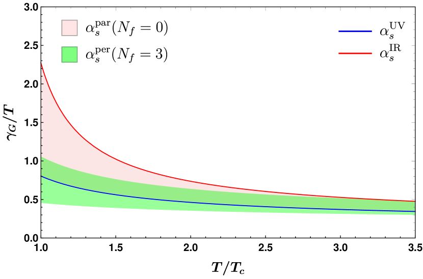
Figure 1: The temperature dependence of the scaled Gribov parameter with $N_{f}=0$ is shown along with the $N_{f}=3$ case obtained considering the asymptotic form and the 1-loop perturbative running. The bands refer to the variation of the scale from $w=w_{\rm IR}$ to $w_{\rm UV}$ and $w=1$ to 4 respectively.

Note that the temperature dependence of the scaled Gribov parameter in the IR case is similar to the decreasing trend obtained using the kinetic theory framework considering the quasiparticle picture of the Gribov plasma [42, 43, 44]. However, unlike the IR scenario, the obtained $\bar{\gamma}_{G}$ for $w=w_{\rm UV}$ remains small throughout the considered temperature range. Moreover, as discussed in Ref. [21], the fitted coupling, along with the obtained $\mu_{0}$, provide an almost temperature-independent ghost dressing function (as obtained from Eq. (27) numerically) which is consistent with the lattice results [45, 46]. However, it should be mentioned that in the original GZ approach, the dressing function shows an IR-enhancement at $P\rightarrow 0$ whereas the recent lattice measurements at vanishing momentum support a finite decoupling behaviour which is in better agreement with the refined GZ approach [28, 29]. Nevertheless, we adopt the original GZ procedure here due to its considerable simplicity compared to the refined GZ approach, especially for finite temperature applications.

It is also interesting to compare the temperature dependence of the Gribov-modified diffusion coefficient with the perturbative result, including the quark contribution. For that purpose, we utilize the asymptotic temperature dependence of the Gribov parameter that can be obtained from the gap equation considering the $T\rightarrow\infty$ limit as

$$\gamma^{\rm asy}_{G}(T) =\frac{d-1}{d}\frac{N_{c}}{4\sqrt{2}\pi}g^{2}(T)T\,.$$ (31)

Thus, the temperature dependence of $\bar{\gamma}_{G}$, in this case, is completely determined by the running coupling. Keeping in mind the functional form of the parametrized coupling for $N_{f}=0$, in this case, we use the one-loop running coupling with $N_{f}=3$, which is given by

$$\alpha^{\rm per}_{s}(T) =\frac{6\pi}{(11N_{c}-2N_{f})\log\left[w(\pi T)/\Lambda_{\rm\overline{MS}}\right]}\leavevmode\nobreak\ ,$$ (32)

where, $\Lambda_{\rm\overline{MS}}=0.176$ GeV is obtained from the lattice measurement $\alpha_{s}(1.5{\rm GeV},N_{f}=3)=0.326$ [47] and we consider $T_{c}=0.16$ GeV to express the running coupling in terms of the scaled temperature $T/T_{c}$. The uncertainty band, in this case, is obtained by varying the energy scale symmetrically around $2\pi T$ by a factor of two (i.e. $1\leq w\leq 4$). As can be observed from Fig. 1, with $N_{f}=3$, where the asymptotic form of the Gribov parameter is considered, the temperature dependence becomes similar to the UV case obtained previously with $N_{f}=0$. In the following, we consider the two scenarios with $N_{f}=0$ and three and discuss the influence of the temperature dependence of the Gribov parameter on the estimation of the heavy quark diffusion coefficient.

IV Numerical estimation of the diffusion coefficient

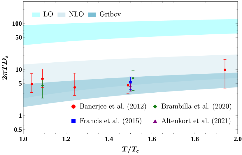
Figure 2: The spatial diffusion coefficient $(2\pi T)D_{s}$ as a function of the scaled temperature is compared with the lattice data from Refs. [10, 12, 13, 14]. At $T=1.5T_{c}$, a horizontal shift is introduced in the data for visual clarity. The bands refer to the variation of the scale parameter from $w=1$ to 4 and $w_{\rm IR}$ to $w_{\rm UV}$ for the LO/NLO and the Gribov case, respectively.

To estimate the temperature dependence of the diffusion coefficient in the GZ framework, one has to perform the momentum integral in Eq. (17) numerically. Let us first consider the pure gluonic background. In that case, the non-trivial temperature dependence of the Gribov mass parameter (see Fig. 1) is obtained by numerically solving Eq. (26) along with the parametrized running coupling given in Eq. (30). The scaled spatial diffusion coefficient, $(2\pi T)D_{s}$, can be obtained from the momentum diffusion coefficient ($\kappa$) by using the Einstein relation $(2\pi T)D_{s}=(4\pi T^{3})/\kappa$.

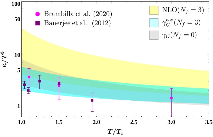
Figure 3: The scaled momentum diffusion coefficient with the asymptotic Gribov parameter is compared with the NLO result considering the 1-loop perturbative running coupling with $N_{f}=3$. The bands refer to the variation of the scale ($w\,\pi T$) from $w=1$ to 4. The Gribov case with $N_{f}=0$ and the lattice data from [10] and [13] are also shown for comparison.

The variation of the obtained $(2\pi T)D_{s}$ as a function of the scaled temperature $T/T_{c}$ is shown in Fig. 2 along with the lattice estimations from Refs. [10, 12, 13, 14]. The uncertainty band, in this case, refers to the variation of the scale ($wT$) obtained by varying the fit parameter $w$ in the range $w_{\rm IR}$ to $w_{\rm UV}$. The corresponding values of the Gribov parameter (as shown in Fig.1) in each of the cases are obtained by solving the gap equation given in Eq. (26). It should be mentioned here that because of this variation of the Gribov parameter with $w$, the error band in the diffusion coefficient deviates from the trivial uncertainty expected from the overall multiplicative factor (see, for example, Eq. (17) with the overall $g^{4}$ factor). Similar reasoning also applies to the known LO and NLO expressions where the Debye mass $m_{D}$ varies with the parameter $w$. As can be noticed from Fig. 2, the temperature dependence of the Gribov-modified diffusion coefficient shows a reasonable agreement with the lattice estimations within the uncertainties. Moreover, the linearly increasing nature of the scaled spatial diffusion coefficient is consistent with the data-driven approach [18, 48] where a linearly increasing parametrization is usually implemented for the non-perturbative soft-part to compare the model output to the experimental data of the heavy-meson nuclear modification factor $R_{AA}$ and the elliptic flow $v_{2}$. As shown in Fig. 2, the Gribov-modified approach significantly corrected the LO result. However, the behaviour of the Gribov improved spatial diffusion coefficient is qualitatively similar to the result obtained incorporating the NLO correction, which is also shown in Fig. 2 for comparison. In this case, the approximate expression for the two-loop perturbative running [49] is used in Eq. (18) along with $T_{c}/\Lambda_{\rm\overline{MS}}=1.15$ [50] and the uncertainty band is obtained by varying the energy scale symmetrically around $2\pi T$ by a factor of two. An overlap between the uncertainty bands of the NLO result and the Gribov-modified diffusion coefficient estimation can be observed throughout the considered range of temperatures. Nevertheless, one can notice a relatively narrower uncertainty band in the GZ case, which essentially stems from the uncertainties in the lattice determination of the running coupling at finite temperatures [41].

It is also interesting to compare the NLO result and the Gribov modified estimation, including the quark sector contribution. For this purpose, we consider the perturbative one loop running coupling given in Eq. (32) (with the energy scale ($w\,\pi T$) varied considering $1\leq w\leq 4$) along with the simple asymptotic temperature dependence of the Gribov parameter (proportional to the chromo-magnetic scale) as given in Eq. (31). Note that the asymptotic temperature dependence of the Gribov parameter has been considered earlier in the studies of the fermion dispersion relation [34] and the dilepton production rate [37] in the GZ framework. In the present case, we incorporate this asymptotic form of the Gribov parameter in Eq. (17) to obtain the corresponding temperature dependence of the scaled momentum diffusion coefficient as shown in Fig 3. For comparison, the Gribov modified result with $N_{f}=0$ is also shown along with the pure glue lattice data from Refs. [10, 13]. It can be observed that the asymptotic form of the Gribov parameter with $N_{f}=3$ gives rise to an almost similar temperature dependence as obtained by solving the gap equation with the parametrized coupling in the $N_{f}=0$ case. Here also, an overlap between the uncertainty bands corresponding to the NLO correction and the Gribov-modified results can be observed throughout the considered temperature range. However, concentrating on a fixed energy scale $2\pi T$ for both cases, one can infer that, close to the critical temperature, the Gribov modified analysis indicates a smaller momentum diffusion coefficient value than the NLO estimation.

V Summary and outlook

In this work, the heavy quark diffusion coefficient up to the leading order in $1/M$ expansion (where $M$ represents the mass of the heavy quark) has been studied in the phenomenologically relevant temperature regime using the Gribov-Zwanziger prescription. The relevant t-channel matrix amplitude at low momentum transfer has been obtained with the IR-suppressed gluon propagator that depends on the Gribov parameter. For pure gluonic medium, the temperature dependence of this parameter has been obtained by solving the gap equation with a parametrized running coupling adopted from Ref. [21]. On the other hand, for $N_{f}=3$, we consider the asymptotic temperature dependence of the Gribov parameter, which is proportional to the chromo-magnetic scale. The temperature dependencies so obtained have been implemented in the estimation of the momentum diffusion coefficient based on the kinetic theory framework, and the corresponding spatial diffusion coefficient is obtained using the Einstein relation. We find that the Gribov-modified prescription significantly improves the LO estimation of the spatial diffusion coefficient resulting in a linearly increasing temperature dependence consistent with the lattice estimations as well as the data-driven approaches. For both $N_{f}=0$ and $N_{f}=3$ cases, the estimated diffusion coefficients in the Gribov approach and the NLO perturbative approach overlap within the uncertainties (though with reduced uncertainties in the former approach). Considering the median of the uncertainty bands with $N_{f}=3$, we find that, near the transition temperature, the GZ approach results in a smaller momentum diffusion coefficient (closer to the value obtained in the pure glue scenario) compared to the NLO estimation.

Note that the present study implements the original GZ approach for the simplicity of incorporating finite temperature modifications. A similar analysis based on the refined GZ approach [51] serves as an interesting future direction. Nevertheless, the significant improvement over the LO estimation of the diffusion coefficient obtained here (even with the asymptotic temperature dependence of the Gribov parameter) definitely encourages one to investigate the importance of the (chromo)magnetic scale in the estimation of other relevant transport properties of the medium [42, 44] as well as in the transport studies in the presence of non-trivial background [52, 53].

References

- Svetitsky [1988] B. Svetitsky, Diffusion of charmed quarks in the quark-gluon plasma, Phys. Rev. D 37, 2484 (1988).
- Andronic et al. [2016] A. Andronic et al., Heavy-flavour and quarkonium production in the LHC era: from proton–proton to heavy-ion collisions, Eur. Phys. J. C 76, 107 (2016), arXiv:1506.03981 [nucl-ex] .
- Beraudo et al. [2018] A. Beraudo et al., Extraction of Heavy-Flavor Transport Coefficients in QCD Matter, Nucl. Phys. A 979, 21 (2018), arXiv:1803.03824 [nucl-th] .
- Dong et al. [2019] X. Dong, Y.-J. Lee, and R. Rapp, Open Heavy-Flavor Production in Heavy-Ion Collisions, Ann. Rev. Nucl. Part. Sci. 69, 417 (2019), arXiv:1903.07709 [nucl-ex] .
- Zhao et al. [2020] J. Zhao, K. Zhou, S. Chen, and P. Zhuang, Heavy flavors under extreme conditions in high energy nuclear collisions, Prog. Part. Nucl. Phys. 114, 103801 (2020), arXiv:2005.08277 [nucl-th] .
- Prino and Rapp [2016] F. Prino and R. Rapp, Open Heavy Flavor in QCD Matter and in Nuclear Collisions, J. Phys. G 43, 093002 (2016), arXiv:1603.00529 [nucl-ex] .
- Moore and Teaney [2005] G. D. Moore and D. Teaney, How much do heavy quarks thermalize in a heavy ion collision?, Phys. Rev. C 71, 064904 (2005), arXiv:hep-ph/0412346 .
- Caron-Huot and Moore [2008] S. Caron-Huot and G. D. Moore, Heavy quark diffusion in perturbative QCD at next-to-leading order, Phys. Rev. Lett. 100, 052301 (2008), arXiv:0708.4232 [hep-ph] .
- Das et al. [2015] S. K. Das, F. Scardina, S. Plumari, and V. Greco, Toward a solution to the and puzzle for heavy quarks, Phys. Lett. B 747, 260 (2015), arXiv:1502.03757 [nucl-th] .
- Banerjee et al. [2012] D. Banerjee, S. Datta, R. Gavai, and P. Majumdar, Heavy Quark Momentum Diffusion Coefficient from Lattice QCD, Phys. Rev. D 85, 014510 (2012), arXiv:1109.5738 [hep-lat] .
- Caron-Huot et al. [2009] S. Caron-Huot, M. Laine, and G. D. Moore, A Way to estimate the heavy quark thermalization rate from the lattice, JHEP 04, 053, arXiv:0901.1195 [hep-lat] .
- Francis et al. [2015] A. Francis, O. Kaczmarek, M. Laine, T. Neuhaus, and H. Ohno, Nonperturbative estimate of the heavy quark momentum diffusion coefficient, Phys. Rev. D 92, 116003 (2015), arXiv:1508.04543 [hep-lat] .
- Brambilla et al. [2020] N. Brambilla, V. Leino, P. Petreczky, and A. Vairo, Lattice QCD constraints on the heavy quark diffusion coefficient, Phys. Rev. D 102, 074503 (2020), arXiv:2007.10078 [hep-lat] .
- Altenkort et al. [2021] L. Altenkort, A. M. Eller, O. Kaczmarek, L. Mazur, G. D. Moore, and H.-T. Shu, Heavy quark momentum diffusion from the lattice using gradient flow, Phys. Rev. D 103, 014511 (2021), arXiv:2009.13553 [hep-lat] .
- Brambilla et al. [2022] N. Brambilla, V. Leino, J. Mayer-Steudte, and P. Petreczky (TUMQCD), Heavy quark diffusion coefficient with gradient flow, (2022), arXiv:2206.02861 [hep-lat] .
- Banerjee et al. [2022] D. Banerjee, R. Gavai, S. Datta, and P. Majumdar, Temperature dependence of the static quark diffusion coefficient, (2022), arXiv:2206.15471 [hep-ph] .
- Cao et al. [2019] S. Cao et al., Toward the determination of heavy-quark transport coefficients in quark-gluon plasma, Phys. Rev. C 99, 054907 (2019), arXiv:1809.07894 [nucl-th] .
- Xu et al. [2018] Y. Xu, J. E. Bernhard, S. A. Bass, M. Nahrgang, and S. Cao, Data-driven analysis for the temperature and momentum dependence of the heavy-quark diffusion coefficient in relativistic heavy-ion collisions, Phys. Rev. C 97, 014907 (2018), arXiv:1710.00807 [nucl-th] .
- Borsanyi et al. [2012] S. Borsanyi, G. Endrodi, Z. Fodor, S. D. Katz, and K. K. Szabo, Precision SU(3) lattice thermodynamics for a large temperature range, JHEP 07, 056, arXiv:1204.6184 [hep-lat] .
- Andersen et al. [2010] J. O. Andersen, M. Strickland, and N. Su, Gluon Thermodynamics at Intermediate Coupling, Phys. Rev. Lett. 104, 122003 (2010), arXiv:0911.0676 [hep-ph] .
- Fukushima and Su [2013] K. Fukushima and N. Su, Stabilizing perturbative Yang-Mills thermodynamics with Gribov quantization, Phys. Rev. D 88, 076008 (2013), arXiv:1304.8004 [hep-ph] .
- Gribov [1978] V. N. Gribov, Quantization of Nonabelian Gauge Theories, Nucl. Phys. B 139, 1 (1978).
- Zwanziger [1989] D. Zwanziger, Local and Renormalizable Action From the Gribov Horizon, Nucl. Phys. B 323, 513 (1989).
- Dokshitzer and Kharzeev [2004] Y. L. Dokshitzer and D. E. Kharzeev, The Gribov conception of quantum chromodynamics, Ann. Rev. Nucl. Part. Sci. 54, 487 (2004), arXiv:hep-ph/0404216 .
- Maas [2013] A. Maas, Describing gauge bosons at zero and finite temperature, Phys. Rept. 524, 203 (2013), arXiv:1106.3942 [hep-ph] .
- Sobreiro and Sorella [2005] R. F. Sobreiro and S. P. Sorella, Introduction to the Gribov ambiguities in Euclidean Yang-Mills theories, in 13th Jorge Andre Swieca Summer School on Particle and Fields (2005) arXiv:hep-th/0504095 .
- Vandersickel and Zwanziger [2012] N. Vandersickel and D. Zwanziger, The Gribov problem and QCD dynamics, Phys. Rept. 520, 175 (2012), arXiv:1202.1491 [hep-th] .
- Dudal et al. [2008] D. Dudal, J. A. Gracey, S. P. Sorella, N. Vandersickel, and H. Verschelde, A Refinement of the Gribov-Zwanziger approach in the Landau gauge: Infrared propagators in harmony with the lattice results, Phys. Rev. D 78, 065047 (2008), arXiv:0806.4348 [hep-th] .
- Capri et al. [2016] M. A. L. Capri, D. Dudal, D. Fiorentini, M. S. Guimaraes, I. F. Justo, A. D. Pereira, B. W. Mintz, L. F. Palhares, R. F. Sobreiro, and S. P. Sorella, Local and BRST-invariant Yang-Mills theory within the Gribov horizon, Phys. Rev. D 94, 025035 (2016), arXiv:1605.02610 [hep-th] .
- Dudal et al. [2017] D. Dudal, C. P. Felix, M. S. Guimaraes, and S. P. Sorella, Accessing the topological susceptibility via the Gribov horizon, Phys. Rev. D 96, 074036 (2017), arXiv:1704.06529 [hep-ph] .
- Gotsman and Levin [2021] E. Gotsman and E. Levin, Gribov-Zwanziger confinement, high energy evolution, and large impact parameter behavior of the scattering amplitude, Phys. Rev. D 103, 014020 (2021), arXiv:2009.12218 [hep-ph] .
- Gotsman et al. [2021] E. Gotsman, Y. Ivanov, and E. Levin, High energy evolution for Gribov-Zwanziger confinement: Solution to the equation, Phys. Rev. D 103, 096017 (2021), arXiv:2012.14139 [hep-ph] .
- Justo et al. [2022] I. F. Justo, A. D. Pereira, and R. F. Sobreiro, Toward background field independence within the Gribov horizon, Phys. Rev. D 106, 025015 (2022), arXiv:2206.04103 [hep-th] .
- Su and Tywoniuk [2015] N. Su and K. Tywoniuk, Massless Mode and Positivity Violation in Hot QCD, Phys. Rev. Lett. 114, 161601 (2015), arXiv:1409.3203 [hep-ph] .
- Linde [1980] A. D. Linde, Infrared Problem in Thermodynamics of the Yang-Mills Gas, Phys. Lett. B 96, 289 (1980).
- Zwanziger [2007] D. Zwanziger, Equation of State of Gluon Plasma from Local Action, Phys. Rev. D 76, 125014 (2007), arXiv:hep-ph/0610021 .
- Bandyopadhyay et al. [2016] A. Bandyopadhyay, N. Haque, M. G. Mustafa, and M. Strickland, Dilepton rate and quark number susceptibility with the Gribov action, Phys. Rev. D 93, 065004 (2016), arXiv:1508.06249 [hep-ph] .
- Combridge [1979] B. L. Combridge, Associated Production of Heavy Flavor States in p p and anti-p p Interactions: Some QCD Estimates, Nucl. Phys. B 151, 429 (1979).
- Berrehrah et al. [2014] H. Berrehrah, E. Bratkovskaya, W. Cassing, P. B. Gossiaux, J. Aichelin, and M. Bleicher, Collisional processes of on-shell and off-shell heavy quarks in vacuum and in the Quark-Gluon-Plasma, Phys. Rev. C 89, 054901 (2014), arXiv:1308.5148 [hep-ph] .
- Gracey [2006] J. A. Gracey, Two loop correction to the Gribov mass gap equation in Landau gauge QCD, Phys. Lett. B 632, 282 (2006), [Erratum: Phys.Lett.B 686, 319–319 (2010)], arXiv:hep-ph/0510151 .
- Kaczmarek et al. [2004] O. Kaczmarek, F. Karsch, F. Zantow, and P. Petreczky, Static quark anti-quark free energy and the running coupling at finite temperature, Phys. Rev. D 70, 074505 (2004), [Erratum: Phys.Rev.D 72, 059903 (2005)], arXiv:hep-lat/0406036 .
- Florkowski et al. [2016a] W. Florkowski, R. Ryblewski, N. Su, and K. Tywoniuk, Transport coefficients of the Gribov-Zwanziger plasma, Phys. Rev. C 94, 044904 (2016a), arXiv:1509.01242 [hep-ph] .
- Florkowski et al. [2016b] W. Florkowski, R. Ryblewski, N. Su, and K. Tywoniuk, Bulk viscosity in a plasma of Gribov-Zwanziger gluons, Acta Phys. Polon. B 47, 1833 (2016b), arXiv:1504.03176 [hep-ph] .
- Jaiswal and Haque [2020] A. Jaiswal and N. Haque, Covariant kinetic theory and transport coefficients for Gribov plasma, Phys. Lett. B 811, 135936 (2020), arXiv:2005.01303 [hep-ph] .
- Cucchieri et al. [2007] A. Cucchieri, A. Maas, and T. Mendes, Infrared properties of propagators in Landau-gauge pure Yang-Mills theory at finite temperature, Phys. Rev. D 75, 076003 (2007), arXiv:hep-lat/0702022 .
- Aouane et al. [2012] R. Aouane, V. G. Bornyakov, E. M. Ilgenfritz, V. K. Mitrjushkin, M. Muller-Preussker, and A. Sternbeck, Landau gauge gluon and ghost propagators at finite temperature from quenched lattice QCD, Phys. Rev. D 85, 034501 (2012), arXiv:1108.1735 [hep-lat] .
- Bazavov et al. [2012] A. Bazavov, N. Brambilla, X. Garcia i Tormo, P. Petreczky, J. Soto, and A. Vairo, Determination of from the QCD static energy, Phys. Rev. D 86, 114031 (2012), arXiv:1205.6155 [hep-ph] .
- Li and Liao [2020] S. Li and J. Liao, Data-driven extraction of heavy quark diffusion in quark-gluon plasma, Eur. Phys. J. C 80, 671 (2020), arXiv:1912.08965 [hep-ph] .
- Beringer et al. [2012] J. Beringer et al. (Particle Data Group), Review of Particle Physics (RPP), Phys. Rev. D 86, 010001 (2012).
- Gupta [2001] S. Gupta, A Precise determination of T(c) in QCD from scaling, Phys. Rev. D 64, 034507 (2001), arXiv:hep-lat/0010011 .
- Canfora et al. [2015] F. E. Canfora, D. Dudal, I. F. Justo, P. Pais, L. Rosa, and D. Vercauteren, Effect of the Gribov horizon on the Polyakov loop and vice versa, Eur. Phys. J. C 75, 326 (2015), arXiv:1505.02287 [hep-th] .
- Fukushima et al. [2016] K. Fukushima, K. Hattori, H.-U. Yee, and Y. Yin, Heavy Quark Diffusion in Strong Magnetic Fields at Weak Coupling and Implications for Elliptic Flow, Phys. Rev. D 93, 074028 (2016), arXiv:1512.03689 [hep-ph] .
- Bandyopadhyay et al. [2022] A. Bandyopadhyay, J. Liao, and H. Xing, Heavy quark dynamics in a strongly magnetized quark-gluon plasma, Phys. Rev. D 105, 114049 (2022), arXiv:2105.02167 [hep-ph] .