MagNet: machine learning enhanced three-dimensional magnetic reconstruction
Abstract
Three-dimensional (3D) magnetic reconstruction is vital to the study of novel magnetic materials for 3D spintronics. Vector field electron tomography (VFET) is a major in house tool to achieve that. However, conventional VFET reconstruction exhibits significant artefacts due to the unavoidable presence of missing wedges. In this article, we propose a deep-learning enhanced VFET method to address this issue. A magnetic textures library is built by micromagnetic simulations. MagNet, an U-shaped convolutional neural network, is trained and tested with dataset generated from the library. We demonstrate that MagNet outperforms conventional VFET under missing wedge. Quality of reconstructed magnetic induction fields is significantly improved.
I Introduction
Recent studies of novel magnetic materials with topological textures, such as skyrmionic families Back et al. (2020); Göbel et al. (2021); Yu et al. (2011); Zheng et al. (2017), become an important driving force in spintronics to develop next generation nano-electronic devices Fert et al. (2017); Hirohata et al. (2020). In addition to two-dimensional (2D) topological textures, their three-dimensional (3D) counterparts are emergent, such as the skyrmion bundle and magnetic hopfion Tang et al. (2021); Liu et al. (2020). 3D magnetic textures are prominent due to their potentially larger volume-density and novel dynamics. However, imaging a 3D magnetic configuration is a major obstacle. Most existing magnetic imaging tools such as Kerr microscopy Scheinfein et al. (1990), magnetic force microscopy Schwarz and Wiesendanger (2008), and spin-polarized scanning tunneling microscopy Wiesendanger (2009) can only resolve magnetic configurations on the 2D surface of a sample. Recent advances in 3D magnetic imaging have been made. Neutron scattering Rossat-Mignod et al. (1991); Mook et al. (1993); Mühlbauer et al. (2019), magnetic X-ray dichroism Thole et al. (1992); van der Laan (1999); Donnelly et al. (2017); Hierro-Rodriguez et al. (2020) and Lorentz transmission electron microscopy (LTEM) De Graef (2009) can probe the internal magnetic structure of a sample. Compared to neutron scattering and X-ray dichroism, LTEM and its derivatives can achieve sub-Angstrom Kisielowski et al. (2008) resolution without accelerating particles with a synchrotron. It is thus attractive to enable LTEM-based 3D magnetic reconstructions.
3D vector field electron tomography (VFET), i.e. 3D magnetic reconstruction from electron phase shifts retrieved from electron holography (EH) Midgley and Dunin-Borkowski (2009) or transport of intensity (TIE) equation Volkov et al. (2002),is a relatively new but fast developing 3D magnetic imaging technique. Compared to LTEM, phase retrieval in EH significantly elevates the spatial resolution of the imaging. Since its earliest proposal by Lai in 1994 Lai et al. (1994), the theoretical foundation of VFET has been established Stolojan et al. (2001); Lade et al. (2005); Phatak et al. (2008). Once clean electron phase shifts of two orthogonal and complete tilt series are collected, two components of the magnetic induction field can be reconstructed separately by the central slicing theorem in scalar tomography. The third component of can then be calculated by the constraint . Thus conventional analytical algorithms, such as weighted backprojection method (WBP) and regridding reconstruction method (Gridrec) can be directly extended to VFET Phatak and Gürsoy (2015). However, in real experiments, there are many sources of inevitable errors during electron phase shifts collection, such as noise, sparsity, misalignment, and missing wedge. Those errors thus lead to significant inevitable artefacts. Iterative algorithms such as algebraic reconstruction technique (ART) and simultaneous iterative reconstruction technique(SIRT), as the second generation of reconstruction algorithms, show the capability of working with data with missing-wedge problem and sparse sampling problem Phatak and Gürsoy (2015). Recent advances of iterative algorithms, such as model based iterative reconstruction (MBIR) Prabhat et al. (2017); Mohan et al. (2018), incorporate with physical knowledge and geometrical information of the sample as prior knowledge and can reconstruct the three components simultaneously. But iteratively minimizing a cost function has to pay a price of eight times longer run-time compared to conventional analytical methods Mohan et al. (2018).
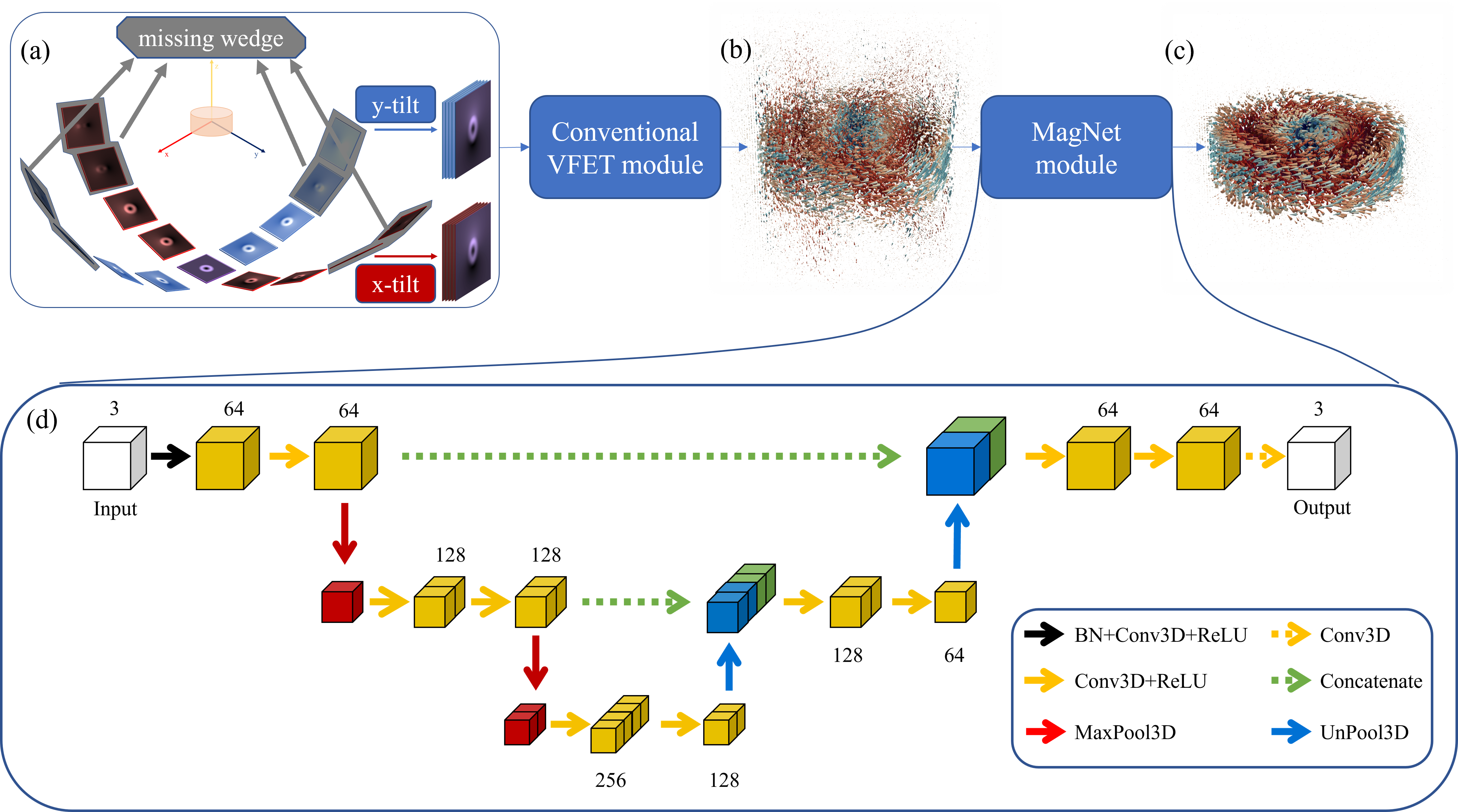
(a) Limited-angle phase shifts of and tilt series. Gray images indicate phase shifts within missing wedge. (b) Conventional VFET reconstructed . (c) MagNet enhanced . (d) The neural network architecture of MagNet. Every convolutional layer is labeled with it’s output channel number.
With the development of machine learning techniques, deep learning tomography (DLT) is emergent as the third generation reconstruction algorithm. Model with Unet Ronneberger et al. (2015) architecture has already shown its capability in removing artefacts in limited-angle tomography Gu and Ye (2017). Instead of building an end-to-end DLT algorithm, combining conventional reconstruction with deep learning is an alternative approach to improve the reconstruction results Adler and Öktem (2018).
In this article, we are focusing on solving the missing-wedge problem in VFET by a DLT algorithm. By attaching an Unet architecture machine learning model to conventional VFET, we build a data-driven DLT algorithm that can work end-to-end from phase shifts to .
We will start section II with the theoretical background and dataflow of our reconstruction model followed by a description of our MagNet architecture. Details about training and testing samples generation as well as the creation of 3D magnetic textures library will also be discussed in this section. In section III, reconstruction results will be shown with comparison to the conventional method. Model performance at different missing-wedge conditions are also discussed there. Conclusions and outlook will be discussed in section IV.
II Theoretical Background, Network architecture, Data Library and Model training
Our MagNet framework is shown in Figure 1. Limited angle phase shifts first enter a VFET module. At the presence of missing wedge, the VFET module gives a defective reconstructed magnetic induction field noted as . is then fed to the Unet module. Unet module outputs an enhanced reconstruction result noted as .
In the VFET module, the projected components of the magnetic induction are the gradient of the phase along orthogonal directions Phatak et al. (2008),
| (1) | ||||
where is the phase shift, is electron charge, and is the Planck constant. Because component is invariant under the rotation about -axis and component is invariant under the rotation about -axis, the reconstruction of and can be simplified as two scalar tomography. In this paper, this tomography is achieved by a simple k-space bilinear interpolation Brynolfsson (2010). And the third component is calculated by the constraint . The Unet module inherits the 3D-Unet skeleton Çiçek et al. (2016). Convolution blocks are used to extract features. The unpool layer is concatenated with skip layer to return the same dimension as the input. Details of our Unet architecture are shown in Figure 1 (e).
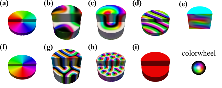
The geometry of magnetic textures are set as cylinders with radius of 40 pixels and thickness varying from 10 to 80 pixels. The majority of magnetic structures in our library are generated from micromagnetic software JuMag.jl Wang by setting various simulating parameters and initial states. Magnetic textures are then manually selected from simulation results to make sure that sample balance and diversity are taken care of. Those micromagnetic structures include vortices, skyrmions, skyrmion lattices, spin helix, conical structures, cylindrical domains, and Néel domain structures. Additionally, manually settled Néel vortices and single domain structures are also added to the library. Representative samples of each category are shown in Figure 2. It shows the diversity of our library despite the library size is only 210. The whole library is divided into a training set with 150 samples, and a testing set with 60 samples. Phase shifts for each sample with maximum tilt angle of , , , and are used as the input of the VFET module under different missing wedge conditions. The tilt angle step is fixed at .
The mean squared error (MSE) of the pixel-wise value difference between the output and the ground truth is chosen as the loss function:
| (2) |
where is the field-of-view (FOV) pixels of the input and the output. Adam optimizer with learning rate is used to update the weights and bias during training. The Unet module is built with Keras framework Chollet et al. (2015). The training was carried out on a single NVIDIA Tesla V100-SXM2-16GB graphic card. One epoch takes about 329 seconds. It takes 100 epochs to get MagNet model ready to use.
III results and discussion
We evaluate the quality of real-space field reconstruction by normalized root mean square error (NRMSE), defined as:
| (3) |
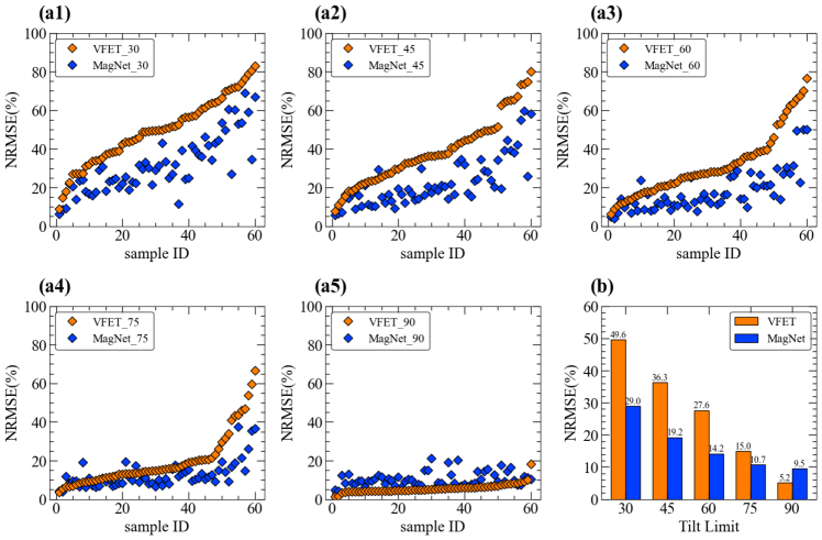
where V is the count of summed pixels. Because the shapes of testing samples are not the same, only pixels inside the material body are taken into account. The VFET result from degree tilt series are noted as VFET_x, and the corresponding MagNet prediction are noted as MagNet_x.
Figure 3 (a1)-(a5) show the NRMSE distribution of VFET and MagNet when the maximum tilt angles are 30, 45, 60, 75 and 90, respectively. The reconstruction is performed in noise-free situation. All samples are sorted by their NRMSEs of VFET from low to high. The NRMSEs of VFET are shown in orange dots, and the NRMSEs of MagNet are shown in blue dots. For example, an orange dot above a blue dot indicates VFET has a higher NRMSE than MagNet for a certain testing sample. It can be found that the blue dots are generally below the orange dots in low tilt limit situation (30, 45, and 60). The advantage becomes less as the tilt limit rises to 75. And when the tilt series is complete, MagNet has a higher NRMSE than VFET.
The NRMSE distribution also shows that the influence of tilt limit varies from sample to sample. For example, the NRMSEs of are distributed between and . For such a wide distribution, we use the median value for evaluating the reconstruction quality, as shown in Figure3 (b). The median NRMSEs of VFET are , , , and when the tilt limits are 30, 45, 60, 75 and 90. And those of MagNet are , , , and , respectively. This metric also shows that MagNet has a better performance except when the tilt series is complete.
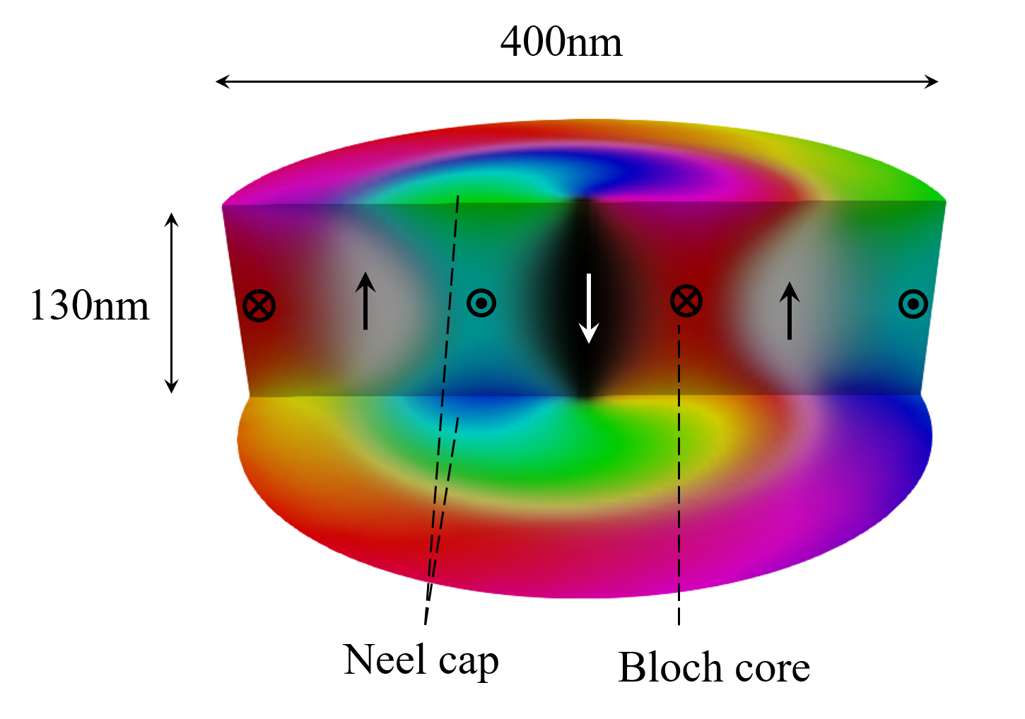
We use a skyrmion sample as a demo to show the comparison between reconstruction results from MagNet and VFET. Figure 4 shows the upper and bottom surfaces, as well as the profile of the 3D magnetic texture. The skyrmion center is along the direction. Similar to the simulation in the previous workMontoya et al. (2017), the domain wall is Bloch-like in the central layers and becomes more Néel-like as approaching surfaces. The diameter and thickness of the disc are 400nm and 130nm, respectively.
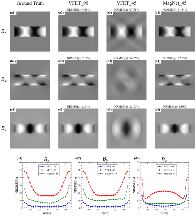
Figure 5 shows the reconstruction results on section. The ground truth, VFET_90 (complete tilt series), VFET_45 and MagNet_45 are shown in the first to the fourth columns, and , and components are shown in the first to the third rows, respectively. Each figure is titled with the NRMSE of corresponding component at x=0 layer. Figures of the same row share a same color scale with the ground-truth image. It shows that all three components of VFET_45 suffer a blurred boundary caused by the missing wedge, while the boundary of MagNet_45 is sharp and clean. The NRMSEs of the three components at x=0 layer are reduced from , , and to , , and , respectively. Figure 5(d1)-(d3) show the single-layer NRMSE of three components at different z coordinates. It shows that the NRMSE improvement of MagNet_45 compared with VFET_45 is about 5% to 30% at different layers.
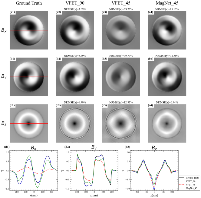
Figure 6 shows the reconstructed results and the ground truth on layer. It shows that the Néel cap is reconstructed by VFET_90, but is not reconstructed by VFET_45. This indicates that the information that constructs the Néel cap is mostly within the missing wedge. With the help of MagNet, the Néel cap can be reconstructed. The NRMSEs of and are significantly reduced from and to and . Figure 6(d) shows a comparison of reconstruction results from different models and ground-truth, indicating obvious enhancements on the and components.
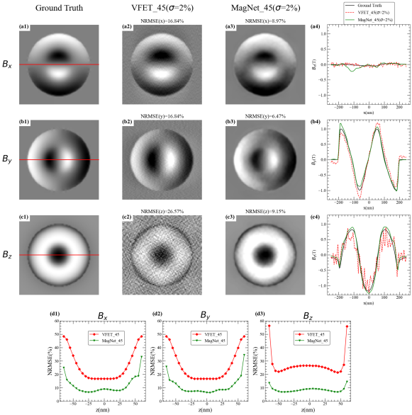
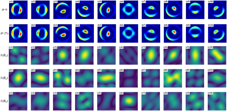
Figure 7 shows the reconstruction results when the phases are contaminated by Gaussian noise. The slice of the ground truth, VFET_45 and MagNet_45 are shown in the first to the third column, respectively. The line profiles are shown in the fourth column. The NRMSEs of and are both , and the NRMSE of is . With the presence of noise, MagNet still keeps a stable performance, and the NRMSE of the three components are only , , and . Figure 7(d1-d3) show the single-layer NRMSE of the three components. Compared with its counterpart in the noise-free situation, the NRMSE of VFET_45 of component has much more increase than that of and . On the other hand, the NRMSE increase of MagNet is tiny, which indicates the noise robustness of MagNet.
When is calculated by the gradient operator which is a high-pass filter in x and y directions, the reconstruction errors of and are linearly amplified with the frequency in x and y directions, respectively. In real experiments, the noise amplification could be suppressed by applying low-pass filters such as Butterworth-type filter Wolf et al. (2022). However, the choice of filter function is empirical, and different filters could lead to very different results. Moreover, k-space filters are also required to reconstruct and . If the relationship between components is considered, the choice of filter for each component would be rather complicated.
On the other hand, the convolutional layer(CL) of MagNet can be regarded as several multi-channel k-space filters. For a CL with input channel number , the tensor in the output channel is:
| (4) |
where and donates the input channel and the output channel respectively, donates the convolution operator, and is the convolution kernel between those two channels. In other words, every output channel accepts information from all input channels. For example, the first CL of MagNet accepts , and as input, so the 64 output features correspond to 64 different combinations of filtered , and . Figure 8(a) and (b) show the slice of top 10 most strongly activated features of MagNet’s first CL with ReLU activation function from noise-free input and noisy input. slice of Fourier amplitude of corresponding convolution kernel are shown in (c)-(e). Taking the strongest output feature as an instance, the Fourier amplitude of (shown in (d1)) is much stronger than that of (shown in (c1)) and (shown in (e1)). As a result, the activated feature is mainly extracted from component. This complex channel interaction provides rich prior knowledge of the relation between different input components.
IV Conclusion
In conclusion, we proposed MagNet, a deep-learning enhanced VFET method, to reduce the reconstruction error caused by missing wedge problem. The reconstruction quality for all testing samples are significantly improved compared with the conventional method when the maximum tile angle is below . A Bloch-type skyrmion with surface modulation is successfully reconstructed with phase shifts gathered at tilt range. The reconstruction of the given example remains stable in the presence of Gaussian noise. It shows that MagNet is promising for real experimental applications.
To improve the performance of data-driven VFET, establishing a larger data library with classified magnetic structures is of vital importance. A widely accepted library can be used not only for training data-driven reconstruction methods, but also for evaluating the performance of reconstruction methods. During the real-world applications of deep-learning VFET algorithms, users can add specific magnetic structures into the library. Finally, although we displayed the application with only one conventional algorithm, MagNet has the potential to work with any other conventional algorithms of VFET. With proper architecture design, it could also work together with modern X-ray reconstruction algorithms.
Data availability
Data will be made available on request.
acknowledge
We are immensely grateful to Rafal E. Dunin-Borkowski and Fengshan Zheng for providing insight and expertise that greatly facilitate the research. We would also like to thank Daniel Wolf for sharing his experience from his previous work with us during the course of this research.
This work was supported by the Office of Basic Energy Sciences, Division of Materials Sciences and Engineering, U.S. Department of Energy, under Award No. DE-SC0020221; H.D. was supported by the Strategic Priority Research Program of Chinese Academy of Sciences, Grant No. XDB33030100, and the Equipment Development Project of Chinese Academy of Sciences,Grant No. YJKYYQ20180012.
References
- Back et al. (2020) C. Back, V. Cros, H. Ebert, K. Everschor-Sitte, A. Fert, M. Garst, T. Ma, S. Mankovsky, T. Monchesky, M. Mostovoy, et al., Journal of Physics D: Applied Physics 53, 363001 (2020).
- Göbel et al. (2021) B. Göbel, I. Mertig, and O. A. Tretiakov, Physics Reports 895, 1 (2021).
- Yu et al. (2011) X. Yu, N. Kanazawa, Y. Onose, K. Kimoto, W. Zhang, S. Ishiwata, Y. Matsui, and Y. Tokura, Nature materials 10, 106 (2011).
- Zheng et al. (2017) F. Zheng, H. Li, S. Wang, D. Song, C. Jin, W. Wei, A. Kovács, J. Zang, M. Tian, Y. Zhang, et al., Physical review letters 119, 197205 (2017).
- Fert et al. (2017) A. Fert, N. Reyren, and V. Cros, Nature Reviews Materials 2, 1 (2017).
- Hirohata et al. (2020) A. Hirohata, K. Yamada, Y. Nakatani, I.-L. Prejbeanu, B. Diény, P. Pirro, and B. Hillebrands, Journal of Magnetism and Magnetic Materials 509, 166711 (2020).
- Tang et al. (2021) J. Tang, Y. Wu, W. Wang, L. Kong, B. Lv, W. Wei, J. Zang, M. Tian, and H. Du, Nature Nanotechnology 16, 1086 (2021).
- Liu et al. (2020) Y. Liu, W. Hou, X. Han, and J. Zang, Physical review letters 124, 127204 (2020).
- Scheinfein et al. (1990) M. Scheinfein, P. Ryan, J. Unguris, D. T. Pierce, and R. Celotta, Applied physics letters 57, 1817 (1990).
- Schwarz and Wiesendanger (2008) A. Schwarz and R. Wiesendanger, Nano Today 3, 28 (2008).
- Wiesendanger (2009) R. Wiesendanger, Reviews of Modern Physics 81, 1495 (2009).
- Rossat-Mignod et al. (1991) J. Rossat-Mignod, L. Regnault, C. Vettier, P. Burlet, J. Henry, and G. Lapertot, Physica B: Condensed Matter 169, 58 (1991).
- Mook et al. (1993) H. Mook, M. Yethiraj, G. Aeppli, T. Mason, and T. Armstrong, Physical Review Letters 70, 3490 (1993).
- Mühlbauer et al. (2019) S. Mühlbauer, D. Honecker, É. A. Périgo, F. Bergner, S. Disch, A. Heinemann, S. Erokhin, D. Berkov, C. Leighton, M. R. Eskildsen, et al., Reviews of Modern Physics 91, 015004 (2019).
- Thole et al. (1992) B. Thole, P. Carra, F. Sette, and G. van der Laan, Physical review letters 68, 1943 (1992).
- van der Laan (1999) G. van der Laan, Physical review letters 82, 640 (1999).
- Donnelly et al. (2017) C. Donnelly, M. Guizar-Sicairos, V. Scagnoli, S. Gliga, M. Holler, J. Raabe, and L. J. Heyderman, Nature 547, 328 (2017).
- Hierro-Rodriguez et al. (2020) A. Hierro-Rodriguez, C. Quirós, A. Sorrentino, L. M. Álvarez-Prado, J. I. Martín, J. M. Alameda, S. McVitie, E. Pereiro, M. Vélez, and S. Ferrer, Nature communications 11, 1 (2020).
- De Graef (2009) M. De Graef, in European Symposium on Martensitic Transformations (EDP Sciences, 2009) p. 01002.
- Kisielowski et al. (2008) C. Kisielowski, B. Freitag, M. Bischoff, H. Van Lin, S. Lazar, G. Knippels, P. Tiemeijer, M. van der Stam, S. von Harrach, M. Stekelenburg, et al., Microscopy and Microanalysis 14, 469 (2008).
- Midgley and Dunin-Borkowski (2009) P. A. Midgley and R. E. Dunin-Borkowski, Nature materials 8, 271 (2009).
- Volkov et al. (2002) V. Volkov, Y. Zhu, and M. De Graef, Micron 33, 411 (2002).
- Lai et al. (1994) G. Lai, T. Hirayama, A. Fukuhara, K. Ishizuka, T. Tanji, and A. Tonomura, Journal of applied physics 75, 4593 (1994).
- Stolojan et al. (2001) V. Stolojan, R. E. Dunin-Borkowski, M. Weyland, and P. Midgley, in Conference Series-Institute of Physics, Vol. 168 (Philadelphia; Institute of Physics; 1999, 2001) pp. 243–246.
- Lade et al. (2005) S. J. Lade, D. Paganin, and M. J. Morgan, Optics communications 253, 392 (2005).
- Phatak et al. (2008) C. Phatak, M. Beleggia, and M. Graef, Ultramicroscopy 108, 503 (2008).
- Phatak and Gürsoy (2015) C. Phatak and D. Gürsoy, Ultramicroscopy 150, 54 (2015).
- Prabhat et al. (2017) K. Prabhat, K. A. Mohan, C. Phatak, C. Bouman, and M. De Graef, Ultramicroscopy 182, 131 (2017).
- Mohan et al. (2018) K. A. Mohan, K. Prabhat, C. Phatak, M. De Graef, and C. A. Bouman, IEEE Transactions on Computational Imaging 4, 432 (2018).
- Ronneberger et al. (2015) O. Ronneberger, P. Fischer, and T. Brox, in International Conference on Medical image computing and computer-assisted intervention (Springer, 2015) pp. 234–241.
- Gu and Ye (2017) J. Gu and J. C. Ye, arXiv preprint arXiv:1703.01382 (2017).
- Adler and Öktem (2018) J. Adler and O. Öktem, IEEE transactions on medical imaging 37, 1322 (2018).
- Brynolfsson (2010) P. Brynolfsson, “Using radial k-space sampling and temporal filters in mri to improve temporal resolution,” (2010).
- Çiçek et al. (2016) Ö. Çiçek, A. Abdulkadir, S. S. Lienkamp, T. Brox, and O. Ronneberger, in International conference on medical image computing and computer-assisted intervention (Springer, 2016) pp. 424–432.
- (35) W. Wang, “Jumag.jl: A julia package for classical spin dynamics and micromagnetic simulations with gpu support.” https://github.com/ww1g11/JuMag.jl.
- Chollet et al. (2015) F. Chollet et al., “Keras,” (2015).
- Montoya et al. (2017) S. Montoya, S. Couture, J. Chess, J. Lee, N. Kent, D. Henze, S. Sinha, M.-Y. Im, S. Kevan, P. Fischer, et al., Physical Review B 95, 024415 (2017).
- Wolf et al. (2022) D. Wolf, S. Schneider, U. K. Rößler, A. Kovács, M. Schmidt, R. E. Dunin-Borkowski, B. Büchner, B. Rellinghaus, and A. Lubk, Nature nanotechnology 17, 250 (2022).