To Softmax, or not to Softmax: that is the question when applying Active Learning for Transformer Models

Abstract

Despite achieving state-of-the-art results in nearly all Natural Language Processing applications, fine-tuning Transformer-based language models still requires a significant amount of labeled data to work. A well known technique to reduce the amount of human effort in acquiring a labeled dataset is Active Learning (AL): an iterative process in which only the minimal amount of samples is labeled. AL strategies require access to a quantified confidence measure of the model predictions. A common choice is the softmax activation function for the final layer. As the softmax function provides misleading probabilities, this paper compares eight alternatives on seven datasets. Our almost paradoxical finding is that most of the methods are too good at identifying the true most uncertain samples (outliers), and that labeling therefore exclusively outliers results in worse performance. As a heuristic we propose to systematically ignore samples, which results in improvements of various methods compared to the softmax function.

Keywords Active Learning  $\cdot$ Transformer  $\cdot$ Softmax  $\cdot$ Uncertainty  $\cdot$ Calibration  $\cdot$ Deep Neural Networks

1 Introduction

The most common use case of Machine Learning (ML) is supervised learning, which inherently requires a labeled dataset to demonstrate the desired outcome to the to-be-trained ML model. This initial step of acquiring a labeled dataset can only be accomplished by often rare-to-get and costly human domain experts; automation is not possible as the automation via ML is exactly the task which should be learned. For example, the average cost for the common label task of segmenting a single image reliably is 6,40 USD. At the same time, recent advances in the field of Neural Network (NN) such as Transformer [Va17] models for Natural Language Processing (NLP) (with BERT [De19] being the most prominent example) or Convolutional Neural Networks (CNN) [LBH15] for computer vision resulted in huge Deep NN which require even more labeled training data. Reducing the amount of labeled data is therefore a primary objective of making ML more applicable in real-world scenarios.

Besides artificially increasing the amount of labeled data by data augmentation, or partially automating the labeling tasks for example through programmatic labeling functions [Ra17], the process of selecting out of the large pool of unlabeled data which samples to label first, called Active Learning (AL), is the target to be improved in this work. AL is an iterative process, in which in each iteration a new subset of unlabeled samples is selected for labeling using human annotators. Due to the iterative selection, the already existent knowledge of the so-far labeled data can be leveraged to select the most promising samples to be labeled next. The goal is to reduce the amount of necessary labeling work while keeping the same model performance.

Despite successful application in a variety of domains, AL fails to work for very deep NN such as Transformer models, rarely beating pure random sampling. The common explanation [Ka21, GI22, SWF22, DD22] is that AL methods favor hard-to-learn samples, often simply called outliers, which therefore neglects the potential benefits from AL. An additional possible explanation is the potential misuse of the softmax activation function of the final output layer as a method for computing the confidence of the NN in its predictions.

Nearly all AL strategies rely on a method measuring the certainty of the to-be-trained ML model in its prediction as probabilities. The reasoning behind is that those samples with high model uncertainty are the most useful ones to learn from, and should therefore be labeled first. For NN typically the softmax activation function is used for the last layer, and its output interpreted as the probability of the confidence of the NN. But interpreting the softmax function as the true model confidence is a fallacy [PBZ21]. We compare therefore eight alternative methods for AL in an extensive end-to-end evaluation of fine-tuning Transformer models for seven common classification datasets AL.

Our main contributions are: 1) comprehensive comparison and evaluation of eight alternative methods to the vanilla softmax function for calculation NN model certainty in the context of AL for fine-tuning Transformer models, and 2) proposing the novel and easy to implement method Uncertainty Clipping (UC) of mitigating the negative effect of uncertainty based AL methods of favoring outliers.

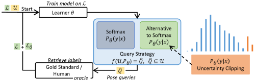
Figure 1: Standard Active Learning Cycle including our proposed Uncertainty Clipping (UC) to influence the uncertainty based ranking (using the probability $P_{\theta}(y|x)$ of the learner model $\theta$ in predicting class $y$ for a sample $x$) by ignoring the top-$k$ results

The remainder of this paper is structured as follows: In Section 2 we briefly explain AL, the Transformer model architecture, and the softmax function. Section 3 presents the alternative confidence measurement techniques, Section 4 describes our experimental setup. Results are discussed in Section 5. In Section 6 we present related work and conclude in Section 7.

2 Active Learning 101

Supervised learning techniques inherently rely on an annotated dataset dataset. AL is a well-known technique for saving human effort by iteratively selecting exactly those unlabeled samples for expert labeling that are the most useful ones for the overall classification task. The goal is to train a classification model $\theta$ which maps samples $x\in\mathcal{X}$ to a respective label $y\in\mathcal{Y}$; for the training, the labels $\mathcal{Y}$ have to be provided “somehow”. Figure 1 shows a standard pool-based AL cycle: Given a small initial labeled dataset $\mathcal{L}=\{(x_{i},y_{i})\}_{i=0}^{n}$ of $n$ samples $x_{i}\in\mathcal{X}$ and the respective label $y_{i}\in\mathcal{Y}$ and a large unlabeled pool $\mathcal{U}=\{x_{i}\},x_{i}\not\in\mathcal{L}$, an ML model called learner $\theta:\mathcal{X}\mapsto\mathcal{Y}$ is trained on the labeled set.

A query strategy $f\colon\mathcal{U}\longrightarrow Q$ then subsequently chooses a batch of $b$ unlabeled samples $Q$, which will be labeled by the oracle (human expert) and added to the set of labeled data $\mathcal{L}$. This AL cycle repeats $\tau$ times until a stopping criterion is met.

In its most basic form, the focus of the sampling criteria is on either informativeness/uncertainty, or representativeness/diversity. Informativeness in this context prefers samples, which reduce the error of the underlying classification model by minimizing the uncertainty of the model in predicting unknown samples. Representativeness aims at an evenly distributed sampling in the vector space of the samples. As we are interested in improving the core measure of informativenesses, the confidence of the ML model in its own predictions, we are concentrating in this paper on evaluating AL strategies, which are solely relying on the informativeness metric.

Commonly used AL query strategies, which are relying on informativeness, use the confidence of the learner model $\theta$ to select the AL query. The confidence is defined by the probability of the learner $P_{\theta}(y|x)$ in classifying a sample $x$ with the label $y$. The most simple informativeness AL strategy is Uncertainty Least Confidence (LC) [LG94], which selects those samples, where the learner model is most uncertain about, i.e. where the probability $P_{\theta}(\hat{y}|x)$ of the most probable label $\hat{y}$ is the lowest:

$$f_{LC}(\mathcal{U})=\operatorname*{argmax}_{x\in\mathcal{U}}\left(1-P_{\theta}(\hat{y}|x)\right)$$ (1)

As we are interested in the effectiveness of alternative methods in computing the confidence probability $P_{\theta}$, we are using each method in combination with Uncertainty Least Confidence (LC), which directly relies solely on the confidence without further processing.

3 Confidence Probability Quantification Methods

The confidence probability of an ML model should represent, how probable it is that the prediction is true. For example, a confidence of $70\%$ should mean a correct prediction in $70$ out of $100$ cases. We are using Neural Network (NN)as the ML model. Due to the property of having one as the sum for all components the softmax function is often used as a makeshift probability measure for the confidence of NNs:

$$\sigma(z_{i})=\frac{exp(z_{i})}{\sum^{K}_{j=1}exp(z_{j})},\text{ for }i=1,\dots,K$$ (2)

The output of the last neurons $i$ before entering the activation functions is called logit, and denoted as $z_{i}$, $K$ denotes the amount of neurons in the last layer. But as has been mentioned in the past by other researchers [LPB17, WT22, GI22, SWF22, DD22], the training objective in training NNs is purely to maximize the value of the correct output neuron, not to create a true confidence probability. An inherent limitation of the softmax function is its inability to have – in the theoretical case – zero confidence in its prediction, as the sum of all possible outcomes always equals 1. Previous works have indicated that softmax based confidence is often overconfident [GG16]. Especially NNs using the often used ReLU activation function [Ag18] for the inner layers can be easily tricked into being overly confident in any prediction by simply scaling the input $x$ with an arbitrarily large value $\alpha>1$ to $\tilde{x}=\alpha x$  [PBZ21, HAB19].

We selected seven methods from the literature suitable to quantify the confidence of Deep NNs such as Transformer models. They can be divided into four categories [Ga21]: a) single network deterministic methods, which deterministically produce the same result for each NN forward pass (Inhibited Softmax (IS) [MSK18], TrustScore (TrSc) [Ji18] and Evidential Neural Networks (Evi) [SKK18]), b) Bayesian methods, which sample from a distribution and result therefore in non-deterministic results (Monte-Carlo Dropout (MC) [GG16]), c) ensemble methods, which combine multiple deterministic models into a single decision (Softmax Ensemble [SOS92] ), and d) test-time augmentation methods, which, similarly to the ensemble methods, augment the input samples, and return the combined prediction for the augmented samples. The last category is a subject of future research as we could not find a subset of data augmentation techniques which reliably worked well for our use case among different datasets.

Additionally to the aforementioned categories, the existing softmax function can be calibrated to produce meaningful confidence probabilities. For calibration we selected the two techniques Label Smoothing (LS) [Sz16] and Temperature Scaling (TeSc) [ZKH20].

More elaborate AL strategies like BALD [KAG19] or QUIRE [HJZ10] not only focus on the confidence probability measure, but also make use of the vector space to label a diverse training set, including also regions far away from the classification boundary. As the focus of this paper is on purely evaluating the influence of the confidence prediction methods, we are deliberately solely using the most basic AL strategy Uncertainty Least Confidence.

In the following the core ideas of the individual methods are briefly explained, more details, reasonings, and the exact formulas can be found in the original papers. In the end we are explaining our meta-strategy Uncertainty Clipping, which significantly enhances several confidence probabilities quantification methods.

Inhibited Softmax (Single Network Deterministic Model)

The Inhibited Softmax method [MSK18] is a simple extension of the vanilla softmax function by an additional constant factor $\alpha\in\mathbb{R}$:

$$\sigma(z_{i})=\frac{exp(z_{i})}{\sum^{K}_{j=1}exp(z_{j})+exp(\alpha)}$$ (3)

The constant factor enhances the effect of the absolute magnitude of the single logit value $z_{i}$ on the softmax output. To ensure that the added fraction is not removed during the training process, several changes to the NN have to be made, including: a) removing the bias $b$ from the input of the neuron activation function, and b) extending the loss function by a special evident regularisation term.

TrustScore (Single Network Deterministic Model)

The TrustScore [Ji18] method uses the set of available labeled data to calculate a TrustScore, independent on the NN model. In a first step the available labeled data is clustered into a single high density region for each class. The TrustScore $ts$ of a sample $x$ is then calculated as the ratio between the distance from $x$ to the cluster of the nearest class $c_{closest}$, and the distance to the cluster of the predicted class $\hat{y}$:

$$ts_{x}=\frac{dist(x,c_{closest})}{dist(x,c_{\hat{y}})}$$ (4)

Therefore, the TrustScore is higher when the cluster of the nearest class is further away from the cluster of the most probable class, indicating a potentially wrong classification. The distance metric as well as the calculation of the clusters is based on the $k$-nearest neighbors algorithm.

Evidential Neural Networks (Single Network Deterministic Model)

Evidential Neural Networks [SKK18] treat the vanilla softmax outputs as a parameter set over a dirichlet distribution. The prediction acts as evidence supporting the given parameter set out of the distribution, and the confidence probability of the NN reflects the dirichlet probability density function over the possible softmax outputs.

Monte-Carlo Dropout (Bayesian Method)

Monte-Carlo Dropout [GG16] is a Bayesian method that uses the NN dropout regularization method to construct for “free” an ensemble of the same trained model. Dropout refers to randomly disabling neurons during the training phase, originally with the aim of reducing overfitting of the to-be-trained network. For Monte-Carlo Dropout, the dropout method is applied during the prediction phase. As neurons are disabled randomly, this results in a large Gaussian sample space of different models. Therefore, each model, with differently dropped out neurons, results in a potentially different prediction. Combining the vanilla softmax prediction using the arithmetic mean produces a combined prediction confidence.

Softmax Ensemble (Ensemble Method)

The softmax ensemble approach uses an ensemble of NN models, similar to Monte-Carlo Dropout. The predictions of the ensemble can be interpreted as a vote upon the prediction. The disagreement among the votees acts then as the confidence probability and can be calculated in two ways, either as Vote Entropy (VE), or as Kullback-Leibler Divergence (KLD) [MN98]:

$$VE(x)=-\sum_{i}\frac{V(\hat{y},x)}{K}log\frac{V(\hat{y},x)}{K}$$ (5)

with $K$ being the number of ensemble models, and $V(x,\hat{y})$ denoting the number of ensemble models assigning the class $\hat{y}$ to the sample $x$. The complete equation to calculate the KLD is omitted for brevity. Using an ensemble of softmax models inside of an AL strategy results in the Query-by-committee (QBC) [SOS92] strategy.

Temperature Scaling (Softmax Calibration Method)

Temperature Scaling [ZKH20] is a model calibration method that is applied after the training and changes the calculation of the softmax function by inducing a temperature $T>0$:

$$\sigma(z_{i})=\frac{exp(z_{i}/T)}{\sum^{K}_{j=1}exp(z_{j}/T)}$$ (6)

For $T=1$ the softmax function stays the same as the original version, for values $T<1$ the softmax output of the largest logit is increased, and for values of $T>1$ (which is the recommended case in using Temperature Scaling) the output of the most probable logit is decreased. This has a dampening effect on the overall confidence.

The value for the temperature $T$ is computed empirically using the existent labeled set of samples during application time. The parameter changes therefore for each AL iteration.

Label Smoothing (Softmax Calibration Method)

Label Smoothing [Sz16] removes a fraction $\alpha$ of the loss function per predicted class and distributes it uniformly among the other classes by adding $\frac{\alpha}{K-1}$ to the other loss outputs, with $K$ being the number of classification classes. In contrast to Temperature Scaling Label Smoothing is not applied post-hoc to a trained network, but has a direct influence on the training process due to a changed loss function.

3.1 Uncertainty Clipping

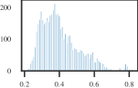
(a) Label Smoothing

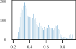
(b) TrustScore

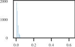
(c) Full Passive Classifier

Figure 2: Exemplary uncertainty values (equals one minus classification confidence probability) for single AL iteration of TREC-6 dataset before Uncertainty Clipping as histograms

The aforementioned methods to quantify the confidence of NNs in their predictions can directly be used in AL strategies to sort the pool of unlabeled samples to select exactly those samples for labeling that have the lowest confidence/highest uncertainty. As repeatedly reported by others [Ka21, GI22, SWF22, DD22], AL is rarely able to outperform pure random sampling when used to fine-tune Transformer models. Purely labeling based on the uncertainty score results in labeling many outliers/hard-to-learn-from samples, which results in an often bad classification performance.

Figure 2 displays exemplarily the histograms of the prediction probabilities/uncertainty values for the two methods Label Smoothing and TrustScore for a single AL iteration for the TREC-6 dataset. Both distributions have a characteristic small peak of uncertainty to the far right, and we theorize, that these are the outliers which are labeled first. For comparison, the uncertainty values of a passive classifier are shown – an NN model trained on the full available training dataset –, such a model is obviously very confident in its predictions.

To prevent this issue we propose the naïve, but powerful method Uncertainty Clipping, where the top-$k\%$ of the most uncertain samples are ignored by the AL strategy, resulting in ignoring the displayed small peaks to the far right. Therefore, not the most uncertain samples – potentially many outliers – but the second-most uncertain samples are labeled. This method can be used in combination with any AL strategy using uncertainty for ranking the pool of unlabeled samples.

4 Experimental Setup

Details to reproduce our evaluation are provided in this chapter. We are open to join the reproducability initiative and to offer other researchers the re-use of our work by making our source code fully publicly available on GitHub .

4.1 Setup

We extended the AL framework small-text [Sc21], tailored for the use-case of applying AL to Transformer networks. Some of the aforementioned methods such as Label Smoothing can be applied directly during the training of the network and have a positive effect on the training outcome, whereas others like Monte-Carlo Dropout are applied after the training is complete. As we are only interested in evaluating the effect of alternative confidence probability quantification methods instead of the potentially positive influence on the classification quality, we are effectively training two Transformer models simultaneously. One is the original vanilla Transformer model with a linear classifier and a softmax on top of the CLS embedding. This one is used for class predictions and for calculating the classification quality. The other one is solely used for the AL selection process, and includes the implemented alternative confidence probability quantification methods. Even though this adds computational overhead to our experiments, it enables us to evaluate the effect of the confidence quantification for AL independently of potentially other positive – or negative – effects on the classification quality.

Parameters for the compared methods were selected empirically using hyper parameter tuning. The constant factor $\alpha$ for Inhibited Softmax was set to $1.0$, for TrustScore the $k$ for the $k$-nearest neighbor calculation to 10. We used an ensemble of $50$ models for Monte-Carlo Dropout, each simple softmax based Transformer model with a different seed for the random-number-generator. For the softmax ensemble we could only use 5 different Transformer models with the vanilla softmax activation function, as the runtime was drastically higher compared to Monte-Carlo Dropout (MC). For Label Smoothing the fraction $\alpha$ was set to $0.2$, and for Temperature Scaling 1.000 different values for $T$ between $0$ and $10$ were tested, the temperature resulting in the smallest cross entropy was finally used. Whenever possible, we used the original implementations of the methods with slight adaptations to make them work together with Transformer models and the small-text framework.

Active Learning Simulation

AL strategy	Abbreviation
Uncertainty Least Confidence (Evidential Neural Networks)	Evi
Uncertainty Least Confidence (Inhibited Softmax)	IS
Uncertainty Least Confidence (Label Smoothing)	LS
Uncertainty Least Confidence (MonteCarlo)	MC
Uncertainty Least Confidence (Softmax Ensemble: Kullback-Leibler Divergence)	KLD
Uncertainty Least Confidence (Softmax Ensemble: Vote Entropy)	VE
Uncertainty Least Confidence (Temperature Scaling)	TeSc
Uncertainty Least Confidence (TrustScore)	TrSc
Random	Rand
Uncertainty Least Confidence (softmax)	LC
Uncertainty Max-Margin (softmax)	MM
Uncertainty Entropy (softmax)	Ent
Passive (full trained set)	Pass

Table 1: Abbreviation for the evaluated AL strategies using the Confidence Probability Quantification Methods including several baselines

To evaluate the effectiveness of the confidence probability methods we are simulating AL in the following way: For a given labeled dataset, we start with an initially labeled set of 25 samples, and perform afterwards 20 iterations of AL, ignoring the known labels for the other samples, following the procedure of [ZLW17] and [SNP22]. In each iteration a batch of 25 samples is selected by the AL strategy for labeling, which is performed using the known ground-truth labels. As AL strategies we used the most simple strategy, directly using the confidence probability measure without further pre-processing for ranking, Uncertainty Least Confidence (see Section 2) in combination with the softmax function replaced with the alternative confidence probability measures. As additional baselines we included Uncertainty Entropy [Sh48], Uncertainty Max-Margin [SDW01] and pure random sampling. The first two further processed the confidence values before ranking by either calculating the entropy of the uncertainty, or calculating the margin between the first and second-most probable class, but did not make use of any other information. Each simulation was repeated 10 times using different initially labeled samples. Another baseline was the passively trained model on all available training data. The used strategies are summarized in Table 1 including their abbreviations used in the plots in the remainder of this paper.

4.2 Transformer Models

A transformer [Va17] is a deep NN model using the self-attention [Va17] mechanism to process sequential input. We use as Transformer models the original $BERT_{base}$ [De19] model and the updated version $RoBERTa_{base}$ [Li19]. The networks of $BERT_{base}$ and $RoBERTa_{base}$ consist of 12 layers with an embedding size of 768, with BERT having 110M parameters, and RoBERTa 125M parameters. We use the pretrained versions from Hugginface [Wo19]. As the AL experiments require a significant amount of fine-tuning the Transformer models we deliberately use the smaller base version instead of the large versions of both Transformer models. Even though the large versions result in presumably better classification accuracies, the relative differences in the compared methods should be nearly the same. Each pre-trained Transformer network is extended by a final fully connected projection layer based on the sentence representation “CLS” token, either using the vanilla softmax function, or using the alternative methods presented in this paper.

4.3 Datasets, Hardware, and Metrics

Dataset Name (abbreviation)	Domain	# classes	#Train	#Test
AG’s News (AG)	News	4	120,000	7,600
CoLA (Co)	Grammar	2	8,551	527
IMDB (IM)	Sentiment	2	25,000	25,000
Rotten Tomatoes (RT)	Sentiment	2	8,530	1,066
Subjectivity (SU)	Sentiment	2	8,000	2,000
SST2 (S2)	Sentiment	2	6,920	1,821
TREC-6 (TR)	Questions	6	5,452	500

Table 2: Information about the datasets used in the experiments.

Table 2 lists the datasets we used in our experiments to fine-tune the pre-trained Transformer models in the AL simulations. The datasets were selected as a diverse set of popular NLP datasets, including binary and multi-class classification of different domains of varying difficulty. The datasets were obtained from the Huggingface dataset repository [Lh21]. We used the train-test-splits provided by Huggingface. All experiments were conducted on a cluster consisting of NVIDIA A100-SXM4 GPUs, AMD EPIC CPU 7352 (2.3GHZ) CPUs and NVMEe disks. Each experiment was run on a single graphic card, with 120GB memory, and 16 CPU cores.

The AL experiments can be evaluated in multitude of ways. At its core, after each AL iteration, a standard ML metric is being measured for the labeled and withheld dedicated test set. We decided upon the accuracy (acc) metric, calculated on a withheld test dataset. It is possible to compare the test accuracy values of the last iteration, the mean of the last five iterations ($acc_{last5}$), and the mean of all iterations. The last one equals the area-under-the-curve when plotting the so-called AL learning curve. As an effective AL strategy should select the most valuable samples for labeling first, those metrics that include the accuracy of multiple iterations are often closer to real use-cases. Nevertheless, at the beginning of the labeling process the fluctuation of the test accuracy for most strategies is very high and contains often surprisingly few information about which strategy is better than another one. The influence of the initially labeled samples is simply so high, that a better strategy, with a bad starting point, has no chance to be better than a bad strategy, which has a good starting point. But after a couple of AL iterations, the results stabilize, and good strategies can be reliably distinguished from bad strategies, as each strategy tends to approach its own characteristic threshold, nevertheless the starting point. We decided therefore to use the accuracy of the last five iterations, deliberately ignoring therefore the first iterations with the highly fluctuating results.

Additionally, we measured the runtime. AL, applied in real-life scenarios, is an interactive process. Decisions of the AL strategy should be made in the magnitude of single-digit seconds, longer calculation times render the annotation process often unusable.

As the experiments were each repeated for 10 times, we display in the following the arithmetic mean for the 10 repetitions.

5 Results

We compared the confidence quantification methods (See Section 3) in many ways: Firstly, we are comparing the test accuracies $acc_{last5}$ of the last five iterations, with and without our proposed Uncertainty Clipping ( 5.1). Secondly, we analyze those samples queried by the AL strategy for labeling to show which strategies behave similarly, indicated by similarly queried samples (Section 5.2. Then, we analyze the class distribution of the queried samples (Section 5.3, and conclude with an analysis of the runtimes (Section 5.4).

5.1 Test Accuracies

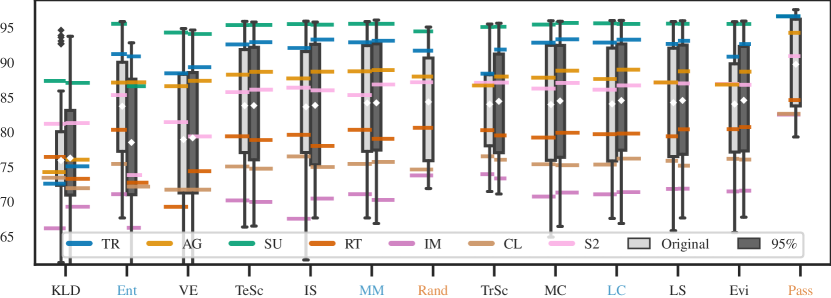
(a) BERT

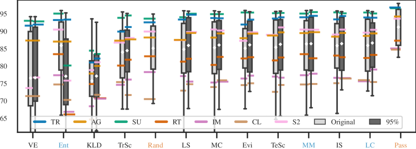
(b) RoBERTa

Figure 3: Distribution of $acc_{last5}$ including the Uncertainty Clipping variants and the average $acc_{last5}$ values per dataset as colorful line, ordered by $acc_{last5}$ after Uncertainty Clipping. The arithmetic mean of the runs per method are included as a white diamond in the middle of the plots. The vanilla softmax based baselines Ent, MM und LC are marked in blue, and the baselines Random Selection as well as the Passive classifier are marked orange.

Figure 3 displays the distributions of the average test accuracy of the last five AL iterations $acc_{last5}$ per method. The light grey boxplot displays the original values, the dark grey the variant with the top-5% of the uncertainty values ignored. The underlying displayed distribution consists of the $acc_{last5}$ values combined for all datasets. As each method was evaluated using 10 different starting points, we additionally display the arithmetic mean of the 10 repetitions per dataset as an additional colorful stick. The methods are ordered after the mean $acc_{last5}$ value using Uncertainty Clipping.

General Remarks

First, it is obvious that the difference between the individual methods differs per dataset, but averaged over all datasets (the white diamond in the middle of the boxplots indicates the arithmetic mean) the differences become marginally small. Still, it can be safely stated already that the Softmax Ensemble techniques (KLD and VE) perform far worse than any other technique.

Uncertainty Clipping

We discarded the top-5% of the most uncertain values when selecting samples for labeling, displayed in the dark grey boxplots. The clipping threshold of 5% was found empirically using hyperparameter tuning, other values up to 10% also worked well. The reasoning behind that is that a good method for calculating confidence probabilities results in an AL strategy querying mostly outliers, as these are the most uncertain values. But solely labeling outliers results in worse performance than Random sampling, as can be seen in Figure 3 when looking only on the light gray boxplots. Our paradoxical finding is therefore that the Softmax function is indeed a bad method for calculating the confidence probability, but purely uncertainty-based AL strategies actually benefit from a slightly worse-than perfect confidence probability method.

Looking purely on the boxplots, Uncertainty Clipping seems to remove some bad performing lower end results from the distributions, and add more better performing. Except for the ensemble methods and Uncertainty Entropy, all methods benefit from Uncertainty Clipping (comparing the overall arithmetic mean of the distributions indicated by the white diamonds). The effect of Uncertainty Clipping becomes more clear if one compares the colorful lines per dataset in each boxplot from the left and the right side. These lines indicate the arithmetic mean per dataset. Especially for the dataset AG-News and Trec-6 the clipping improves the final test accuracy drastically, as the right lines are often higher than the left ones. Some datasets such as AG-News or Trec-6 are more influenced by Uncertainty Clipping, indicating a higher percentage of outliers in these datasets in comparison to datasets such as Subjectivity.

Baselines

In addition to pure Random Sampling selection, and Uncertainty Least Confidence with the vanilla softmax function, Uncertainty Entropy and Uncertainty Max-Margin– both also using the vanilla softmax function – were included in our evaluation. Uncertainty Entropy seems to be the only strategy which is highly negatively influenced by Uncertainty Clipping. Apparently, the calculation of the entropy on top of the softmax negates the negative impact of outliers. The baseline strategies Uncertainty Least Confidence and Uncertainty Max-Margin perform better on RoBERTa than on BERT, indicating that the softmax function is better calibrated to true probabilities for RoBERTa than for the original BERT model.

Best overall performing method

The results differ based on the used Transformer model. In general, no alternative method was able to be better for both models than vanilla softmax used in Uncertainty Least Confidence (LC). Evidential Neural Networks (Evi)seems promising and performs well for both Transformer models, whereas most other strategies, which perform good for one model, perform bad for the other ones. As the differences between the methods are mostly marginal, our results do not allow to rule out Label Smoothing (LS), Monte-Carlo Dropout (MC), Temperature Scaling (TeSc), or TrustScore (TrSc), as these are all close behind. Also, the baseline Uncertainty Max-Margin (MM)seems promising.

5.2 Queried Samples

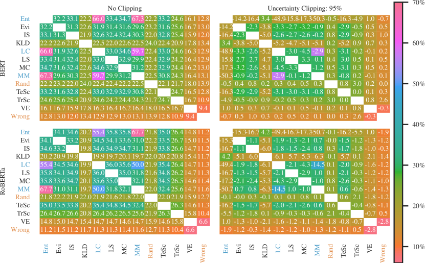
Figure 4: Heatmap for the Jaccard coefficients of the queried samples between each pair of strategies. High coefficients indicate highly similar strategies. On the right side the displayed numbers indicate the difference to the original coefficients.

We are also interested in the similarities and differences of the probability quantification methods. Hence, we calculated the Jaccard coefficients between the sets of queried samples for each pair of compared AL strategies, displayed in Figure 4. As our experiments were repeated 10 times each, we used the union of the sets of queried samples, and the union of the results per dataset. Additionally, we included the wrongly classified samples (wrong) by the passive classifier – potentially being outliers – in the plots. The left side contains the Jaccard coefficients for the version without Uncertainty Clipping, the right side with the top-5% results being ignored. The right side contains the percentual difference to the unclipped version as numbers, whereas the color encoding still indicates the Jaccard coefficient.

For the unclipped version, the most similar strategies are unsurprisingly the three strategies using the pure softmax function: Uncertainty Entropy, Uncertainty Least Confidence, and Uncertainty Max-Margin. As the clipping has a high negative impact on Uncertainty Entropy, it becomes highly dissimilar from almost any other strategy, with a drop of over 40% compared to Uncertainty Least Confidence.

Apart from this, Evidential Neural Networks, Label Smoothing, Monte-Carlo Dropout, Inhibited Softmax, and Temperature Scaling are equally similar to each other in the area of 30%, as has been already been indicated by the similar performance in the previous section. TrustScore is only similar in the area of 25%, and the Softmax Ensemble methods Vote Entropy and Kullback-Leibler Divergence are highly dissimilar to everything else. Also, almost all strategies are, as expected, very dissimilar to pure random selection, and even less similar to the set of wrongly classified samples.

Uncertainty Clipping seems to make all strategies behave less similar, as nearly all Jaccard coefficients go slightly down. This indicates that all strategies without Uncertainty Clipping label the same set of outliers, and after these are removed, they have of course less similarities. We also included the wrongly classified samples (Wrong) by the fully trained passive classifiers in the analysis. Interestingly, a difference can be seen between the two compared Transformer models: for RoBERTa most strategies sample few wrongly classified samples, which becomes even less after the Uncertainty Clipping, whereas for the original BERT model the percentage of queried samples increases slightly with Uncertainty Clipping.

Also, all strategies become slightly more similar to random selection, which is expected, as Uncertainty Clipping removes the best results based on the uncertainty heuristic, leaving the strategies labeling the second-best-results, which are often closer to pure random selection, as the best bets based on the heuristics are removed.

In conclusion, equally good performing strategies also query similar samples, and Uncertainty Clipping manages to remove a set of outliers, which the different methods apparently have in common.

5.3 Class distribution

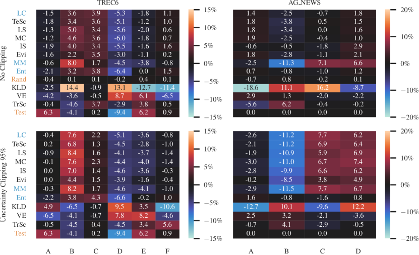
Figure 5: Difference of class distribution of the queried samples compared to the train set for the two datasets TREC-6 and AG’s News for the original BERT model

To further analyze Uncertainty Clipping, we selected the two datasets, TREC-6 and AG’s News, which have more than two target classes, for an additional deeper analysis of difference in class distribution for the queried samples, compared to distribution in the training set, displayed in Figure 5. Additionally, we include the class distribution across the test dataset. The expectation of the random strategy would be the same class distribution in the queried samples as in the full available training dataset, which nearly holds true.

For TREC-6, most strategies favor samples from class B and C, and sample less samples from class D. Uncertainty Clipping simply enhances this behavior. For AG’s News almost all strategies sample evenly distributed among all classes without Uncertainty Clipping, and significantly less often of class B, but more of class C and D with Uncertainty Clipping. Uncertainty Max-Margin stands out from the other methods, as it behaves without clipping similar to all other methods that use clipping. This explains why Uncertainty Max-Margin is one of the few methods that does not benefit from Uncertainty Clipping for Trec-6 and AG’s News, as seen in Figure 3, despite an otherwise good performance.

We infer from the data that Uncertainty Clipping vastly influences the distribution of the queried classes towards potentially more interesting classes for labeling, which are the same for all methods.

5.4 Runtime Comparison

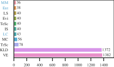
(a) BERT

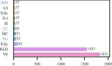
(b) RoBERTa

Figure 6: Runtime Comparison of all methods averaged over the datasets in seconds

AL is in practice an iterative process. Annotators want a responsive systems, which tells them immediately what to label next, without long waiting times. Therefore, a fast runtime of the AL query selection is a crucial factor in making AL real-world usable. We display in Figure 6 the runtimes averaged over all datasets for our methods in seconds per complete AL loop, measuring only the time of the AL computations, not the Transformer model fine-tuning time . First, it becomes clear that the overhead of our Softmax Ensemble methods of training multiple Transformer models in parallel is simply too high. Apart from that, almost all other methods seem to perform equally fast, with Monte-Carlo Dropout and TrustScore as the slightly, but probably neglectable, slowest methods.

6 Related Work

The importance of a good quantification method for prediction confidence probabilities for AL has been noted often before [LPB17, Bl15], especially in the context of deep NN like Transformer models [SNP22]. Nevertheless, few research has been done on solely comparing certainty probability methods, with the goal of AL for Transformer models in mind.

[WT22] compared Uncertainty Max-Margin, Uncertainty Entropy, Monte-Carlo Dropout, as well as DeepGini, a modified softmax version with a fast runtime in mind. The primary focus of their work is on test input prioritizers to work with very large datasets. They conclude that Monte-Carlo Dropout performs better than the other strategies, but not so much that it justifies its usage over the vanilla softmax, and that more research in that area is necessary. In [GI22] the usefulness of softmax ensemble methods for Transformer models was investigated, with the same conclusion as ours: ensemble methods perform far worse than even random sampling for Transformer models. The authors of [SWF22] propose an improved variant to standard Monte-Carlo Dropout, directly extending the Transformer architecture. They also note that it is sometimes better to throw away some labels to improve the accuracy, indicating similar observed results, which led us to the idea of Uncertainty Clipping. On a similar note, [DD22] find that AL methods, when applied to Transformer models, often perform inconsistent due to labeling too many unlearnable outliers. Their solution to the problem is training multiple models, resulting in an ensemble approach. Our runtime comparison indicated that ensemble approaches should be used with caution due to very high runtimes, compared to all other methods. In [Ka21] the authors also noted the highly negative impact of outliers as hard-to-learn-from samples for Transformer models through an extensive ablation study, and propose future research develop methods, to ignore these outliers.

[PBZ21] deeply investigates the foundations of the vanilla softmax function as confidence probability. They aim to explain why it functions surprisingly and state that the softmax function might have a sounder basis than widely believed. Our results support this idea as Uncertainty Least Confidence was not really outperformed by any other method.

7 Conclusion

Noting the importance of NN prediction confidence probability measures, and the potential shortcomings of simply using vanilla softmax as such a measure, we experimentally compared eight alternative methods over seven datasets using both the original BERT Transformer model as well as the improved RoBERTa variant. After discovering that better prediction confidence methods result in selecting only outliers for labeling, we proposed Uncertainty Clipping, improving all methods, including vanilla softmax, which was not outperformed by any proposed method. Our evaluation focused on comparing the set of queried samples, the class distributions, as well as a runtime comparison, enabling us to better understand what Uncertainty Clipping actually changes.

In conclusion, we have not found any evidence preventing us from recommending the vanilla softmax method. Still, the compared methods such as Label Smoothing, Evidential Neural Networks, and Monte-Carlo Dropout are not far behind. Our proposed Uncertainty Clipping improves both vanilla softmax as well as alternative methods, and should be used in practice.

Future research should compare the effectiveness of Uncertainty Clipping in combination with more advance AL strategies, which also make use of the vector space.

References

- [Ag18] Abien Fred Agarap “Deep learning using rectified linear units (relu)” In arXiv preprint arXiv:1803.08375, 2018
- [Bl15] Charles Blundell, Julien Cornebise, Koray Kavukcuoglu and Daan Wierstra “Weight uncertainty in neural network” In ICML, 2015, pp. 1613–1622 PMLR
- [DD22] Mike D’Arcy and Doug Downey “Limitations of Active Learning With Deep Transformer Language Models”, 2022 URL: https://openreview.net/forum?id=Q8OjAGkxwP5
- [De19] Jacob Devlin, Ming-Wei Chang, Kenton Lee and Kristina Toutanova “BERT: Pre-training of Deep Bidirectional Transformers for Language Understanding” In Proceedings of the 2019 Conference of the North American Chapter of the Association for Computational Linguistics: Human Language Technologies, Volume 1 (Long and Short Papers) Association for Computational Linguistics, 2019, pp. 4171–4186 DOI: 10.18653/v1/N19-1423
- [Ga21] Jakob Gawlikowski et al. “A survey of uncertainty in deep neural networks” In arXiv preprint arXiv:2107.03342, 2021
- [GG16] Yarin Gal and Zoubin Ghahramani “Dropout as a bayesian approximation: Representing model uncertainty in deep learning” In ICML, 2016, pp. 1050–1059 PMLR
- [GI22] Adam Gleave and Geoffrey Irving “Uncertainty Estimation for Language Reward Models” In arXiv preprint arXiv:2203.07472, 2022
- [HAB19] Matthias Hein, Maksym Andriushchenko and Julian Bitterwolf “Why relu networks yield high-confidence predictions far away from the training data and how to mitigate the problem” In Proceedings of the IEEE/CVF Conference on Computer Vision and Pattern Recognition, 2019, pp. 41–50
- [HJZ10] Sheng-jun Huang, Rong Jin and Zhi-Hua Zhou “Active Learning by Querying Informative and Representative Examples” In NeurIPS 23 Curran Associates, Inc., 2010, pp. 892–900
- [Ji18] Heinrich Jiang, Been Kim, Melody Guan and Maya Gupta “To Trust Or Not To Trust A Classifier” In NeurIPS 31, 2018
- [Ka21] Siddharth Karamcheti, Ranjay Krishna, Li Fei-Fei and Christopher Manning “Mind Your Outliers! Investigating the Negative Impact of Outliers on Active Learning for Visual Question Answering” In IJCNLP Association for Computational Linguistics, 2021, pp. 7265–7281 DOI: 10.18653/v1/2021.acl-long.564
- [KAG19] A. Kirsch, J. Amersfoort and Y. Gal “BatchBALD: Efficient and Diverse Batch Acquisition for Deep Bayesian Active Learning” In NeurIPS 32 Curran Associates, Inc., 2019, pp. 7026–7037
- [LBH15] Yann LeCun, Yoshua Bengio and Geoffrey Hinton “Deep learning” In nature 521.7553 Nature Publishing Group, 2015, pp. 436–444
- [LG94] David D. Lewis and William A. Gale “A Sequential Algorithm for Training Text Classifiers” In SIGIR ’94 Springer London, 1994, pp. 3–12
- [Lh21] Quentin Lhoest et al. “Datasets: A community library for natural language processing” In arXiv preprint arXiv:2109.02846, 2021
- [Li19] Yinhan Liu et al. “Roberta: A robustly optimized bert pretraining approach” In arXiv preprint arXiv:1907.11692, 2019
- [LPB17] Balaji Lakshminarayanan, Alexander Pritzel and Charles Blundell “Simple and scalable predictive uncertainty estimation using deep ensembles” In NeurIPS 30, 2017
- [MN98] Andrew Kachites McCallumzy and Kamal Nigamy “Employing EM and pool-based active learning for text classification” In ICML, 1998, pp. 359–367 Citeseer
- [MSK18] Marcin Możejko, Mateusz Susik and Rafał Karczewski “Inhibited softmax for uncertainty estimation in neural networks” In arXiv preprint arXiv:1810.01861, 2018
- [PBZ21] Tim Pearce, Alexandra Brintrup and Jun Zhu “Understanding softmax confidence and uncertainty” In arXiv preprint arXiv:2106.04972, 2021
- [Ra17] Alexander Ratner et al. “Snorkel: Rapid training data creation with weak supervision” In Proceedings of the VLDB Endowment. International Conference on Very Large Data Bases 11.3, VLDB, 2017, pp. 269 NIH Public Access
- [Sc21] Christopher Schröder, Lydia Müller, Andreas Niekler and Martin Potthast “Small-text: Active Learning for Text Classification in Python” In arXiv preprint arXiv:2107.10314, 2021
- [SDW01] Tobias Scheffer, Christian Decomain and Stefan Wrobel “Active Hidden Markov Models for Information Extraction” In Advances in Intelligent Data Analysis Springer Berlin Heidelberg, 2001, pp. 309–318
- [Sh48] Claude E. Shannon “A mathematical theory of communication” In Bell Syst. Tech. J. 27.3, 1948, pp. 379–423
- [SKK18] Murat Sensoy, Lance Kaplan and Melih Kandemir “Evidential deep learning to quantify classification uncertainty” In NeurIPS 31, 2018
- [SNP22] Christopher Schröder, Andreas Niekler and Martin Potthast “Revisiting Uncertainty-based Query Strategies for Active Learning with Transformers” In Findings of the Association for Computational Linguistics: ACL 2022, 2022, pp. 2194–2203
- [SOS92] H.. Seung, M. Opper and H. Sompolinsky “Query by Committee”, COLT ’92 Pittsburgh, Pennsylvania, USA: Association for Computing Machinery, 1992, pp. 287–294 DOI: 10.1145/130385.130417
- [SWF22] Karthik Abinav Sankararaman, Sinong Wang and Han Fang “BayesFormer: Transformer with Uncertainty Estimation” In arXiv preprint arXiv:2206.00826, 2022
- [Sz16] Christian Szegedy et al. “Rethinking the inception architecture for computer vision” In Proceedings of the IEEE conference on computer vision and pattern recognition, 2016, pp. 2818–2826
- [Va17] Ashish Vaswani et al. “Attention is all you need” In NeurIPS 30, 2017
- [Wo19] Thomas Wolf et al. “Huggingface’s transformers: State-of-the-art natural language processing” In arXiv preprint arXiv:1910.03771, 2019
- [WT22] Michael Weiss and Paolo Tonella “Simple Techniques Work Surprisingly Well for Neural Network Test Prioritization and Active Learning (Replicability Study)” In arXiv preprint arXiv:2205.00664, 2022
- [ZKH20] Jize Zhang, Bhavya Kailkhura and T Yong-Jin Han “Mix-n-match: Ensemble and compositional methods for uncertainty calibration in deep learning” In ICML, 2020, pp. 11117–11128 PMLR
- [ZLW17] Ye Zhang, Matthew Lease and Byron Wallace “Active discriminative text representation learning” In Proceedings of the AAAI Conference on Artificial Intelligence 31.1, 2017