Probability computation for high–dimensional semilinear SDEs driven by isotropic stable processes via mild Kolmogorov equations
Abstract
Semilinear, dimensional stochastic differential equations (SDEs) driven by additive Lévy noise are investigated. Specifically, given the interest is on SDEs driven by stable, rotation–invariant processes obtained by subordination of a Brownian motion. An original connection between the time–dependent Markov transition semigroup associated with their solutions and Kolmogorov backward equations in mild integral form is established via regularization–by–noise techniques. Such a link is the starting point for an iterative method which allows to approximate probabilities related to the SDEs with a single batch of Monte Carlo simulations as several parameters change, bringing a compelling computational advantage over the standard Monte Carlo approach. This method also pertains to the numerical computation of solutions to high–dimensional integro–differential Kolmogorov backward equations. The scheme, and in particular the first order approximation it provides, is then applied for two nonlinear vector fields and shown to offer satisfactory results in dimension .
Keywords: Kolmogorov equations, Semilinear SDEs, Iterative scheme, Isotropic stable Lévy processes.
MSC2020: 60G52, 60H50, 65C20, 45K05, 47D07.
1 Introduction
In this paper, we are concerned with the study of quantities related to the dimensional, semilinear stochastic differential equation (SDE)
| (1) |
with a specific interest in the case high. Here, given , is an stable subordinator (i.e., an increasing Lévy process) independent from , which in turn are independent Brownian motions; we write . All these processes are defined in a common complete probability space which we endow with the minimal augmented filtration generated by the subordinated Brownian motion . Moreover, is a finite time horizon and is the initial time. As for , they are diagonal matrices with negative–definite and positive–definite. For our numerical experiments we will consider being the identity matrix, so that is a parameter describing the strength of the noise. Finally, the nonlinear bounded vector field is subject to suitable regularity conditions which will be specified in the sequel and guarantee, among other things, the existence of a pathwise unique solution of (1): it will be denoted by .
Connected to the SDE in (1), we have the following Kolmogorov backward equation:
| (2) |
where , is the closed unit ball and we fix . Here is the Lévy measure of , and up to a positive multiplicative constant is of the form (see, e.g., [20, Theorem 30.1]). The link between the equations in (1) and (2) is provided by Theorem 7 below (see also the book [15] for related results), where it is shown that the time–dependent Markov transition semigroup associated with (1) satisfies (2) in the closed interval for every . Moreover, we are able to extend the validity of this connection in to every function through an original procedure based on regularization–by–noise and a mild, integral formulation of (2) (see Remark 1).
In the present work, we are precisely interested in these expected values, with particular attention to the case (for some threshold ), where one has . Hence we want to describe a method which allows to compute probabilities related to the solution of the SDE (1). Trying to get an estimate of them by numerically solving the integro–differential equation (2) is a typical example of curse of dimensionality (CoD), and since we intend to deal with a high dimension (in the simulations we take ), this is an unfeasible way to proceed. The canonical approach to tackle our problem is the Monte Carlo method: several paths of are simulated by the Euler–Maruyama scheme with a fine time step, and then the final points of these trajectories are averaged to get an approximation of the desired expected values by virtue of the strong law of large numbers. However, if we were to follow this scheme (which is known to be free of the CoD), then we would have to start over the procedure every time we change the starting point and the starting time , the noise strength and even the nonlinearity , a practice that is very common in a wide range of applications including weather forecasts and calibration of financial models (see [1] and references therein). In order to overcome this setback, we aim to extend to our framework the ideas developed in the papers [9, 10] for the Gaussian case, namely we search for an iterative scheme which relies on a single bulk of Monte Carlo simulations independent from the aforementioned parameters. Specifically, to approximate the value of the iterates we just need to simulate once and for all, using the Euler–Maruyama scheme, a large number of sample paths of the subordinator and of the stochastic convolution , which is the unique (up to indistinguishability) solution of the linear SDE
The main novelty of the approach that we propose consists in the structure of the noise , which is a stable, rotation–invariant Lévy process (cfr. [20, Example ]). In particular, the introduction of considerably complicates the framework compared to the Brownian one treated in [9, 10]. This fact leads us to develop an original procedure –essentially based on conditioning with respect to the algebra generated by the subordinator– to get an expression for the iterates which is suitable for applications. Moreover, the theoretical foundation of the iterative method analyzed in this work, Theorem 3, has a remarkable interest on its own. Indeed, it establishes a connection between the time–dependent Markov transition semigroup associated with (1) and a mild, integral formulation of (2) (see Equation (11)) that, at the best of our knowledge, is new when it comes to isotropic Lévy processes.
The paper is structured as follows. Section 2 describes the setting and recalls the main concepts that will be widely used in the rest of the paper. In addition, it introduces the integral formulation of the Kolmogorov equation (2) and shows its well–posedness. Next, in Section 3 (see Theorem 3) we provide the probabilistic interpretation of (2) in mild form, along with other interesting regularization–by–noise results for SDEs driven by subordinated Wiener processes. In Section 4 we define the iterative scheme and prove its convergence to the expected values that we are trying to approximate. Next, Section 5 is concerned with the computation of the first iterate ; it is divided into two subsections referring to the deterministic and random time–shifts, respectively. Its results are used in Section 6 as the base case for the induction argument that allows to calculate (see Theorem 17). The last part (Section 7) is devoted to numerical experiments in dimension for two choices of the nonlinear vector field , with particular attention on the improvements provided by the first iteration over the linear approximation corresponding to the Ornstein–Uhlenbeck (hereafter OU) processes. Finally, A contains the proof of Lemma 4.
Notation: Let . In this paper, elements of are columns vectors. For any , we denote by the Euclidean norm and by the standard scalar product. For a matrix is the operator norm. Given a vector field , the uniform norm is . In particular, if then the Jacobian matrix is denoted by , and ; if also (so that is a scalar function) then the gradient is a row vector and represents the Hessian matrix. For an integer , the space is constituted by the continuous vector fields which are bounded, continuously differentiable up to order with bounded derivatives. Taken and , we write , where and is a multi–index with length .
2 Preliminaries and Kolmogorov backward equation in mild form
Fix and a complete probability space . Consider independent Brownian motions : we write . Moreover, for we take a strictly stable subordinator independent from , and denote by the augmented algebra it generates, i.e., , where is the natural algebra generated by and is the family of negligible sets. In other words, is an increasing Lévy process with (cfr. [20, Example ])
| (3) |
Let us introduce the diagonal matrices and , with and . We endow with the minimal augmented filtration generated by , which means for , with being the natural filtration of .
Given and a continuous function , if and then is the OU process starting from at time , i.e., it is the unique solution of the next linear SDE
| (4) |
We denote by the time–dependent, Markov transition semigroup associated with this family of processes:
| (5) |
where denotes the space of real–valued, Borel measurable and bounded functions defined on . The Chapman–Kolmogorov equations ensure that
| (6) |
For every we define and An adaptation of [5, Theorem ] guarantees that, for every , the function is differentiable at any point in every direction , with
| (7) |
Moreover, and the following gradient estimate holds true for some constant :
| (8) |
In the sequel, for every and we are going to need the continuity of in the interval [resp., in the closed interval ] when [resp., ]. In order to prove this property, we first note that a variation of constants formula lets us consider (from (4))
| (9) |
This expression shows that the process is stochastically continuous (in the variable ). As a consequence, if , then we can easily deduce the continuity of in applying the continuous mapping and Vitali’s convergence theorems to (5). In the general case one can use the same argument combined with the regularizing property of and (6) to obtain the continuity of in , as desired. Finally, observe that there exists a constant such that
We refer to [5, Remark ] for a similar computation. Let us assume : in this way, denoting by , we have and the bound in (8) entails
| (10) |
For a given measurable and bounded vector field , we are concerned with the analysis of the following Kolmogorov backward equation in mild, integral form:
| (11) |
where and . We denote by . In order to study (11), for every we consider the Banach space defined by
When , we are careful to remove the left–end point of the interval in the previous definitions, so that we will be working with the space . The following lemma proves the well–posedness of (11). We refer to [8, Theorem ] for an analogous result concerning the Kolmogorov forward equation in mild form associated with OU processes in infinite dimension corresponding to Brownian motions.
Theorem 1.
Let and be a measurable and bounded vector field. Then for every and , there exists a unique solution of (11) such that , where .
Proof.
Let us fix and introduce the map given by
| (12) |
for every . Notice that such an application is well defined and with values in , thanks to the properties of discussed above, the dominated convergence theorem and the next computations based on (10):
| (13) |
Here is the same constant as in (10), and the last inequality is obtained using the bound
| (14) |
where for the second equality we perform the substitution . Estimates similar to those in (13) allow to write, for every ,
Hence we obtain
| (15) |
This shows that, for sufficiently small, the map is a contraction in : we denote by its unique fixed point. Now define
| (16) |
and notice that Therefore is the unique, local solution of (11) (in the strip ) such that
At this point, we can repeat the same procedure to construct the solution of (11) in the interval , because the relation among constants in (15) –which is necessary to get a contraction– does not depend on the initial condition. Specifically, we take and define the map
for every . Computations analogous to the ones in the previous step show that is a contraction: its unique fixed point is denoted by . Then we call
notice that , and that by the definition of , one has . Now we extend the function in (16) assigning
By the Chapman–Kolmogorov equations and Fubini’s theorem we realize that is the unique local solution of (11) (in the strip ) such that In the sequel, we can simply denote it by .
This argument by steps of lenght can be repeated iteratively to cover the whole interval and obtain the unique, global solution of (11) such that . Thus, the proof is complete. ∎
If , then recalling (9) one can directly write . Next, considering that , an application of (7)-(10) shows that with
where is the same constant as in (10). This argument can be iterated to claim that, given an integer and , and
| (17) |
The previous consideration allows to extend Lemma 1. To this purpose, for an integer and we introduce the Banach space defined by
As we have done before, when we remove the left–end point of
Corollary 2.
Let be an integer and . Then for every and , there exists a unique solution of (11) such that where .
Proof.
Take an integer ; the argument parallels the one in the proof of Lemma 1, so here we only show that, for a given and sufficiently small, the map in (12) is well defined and a contraction. First, we note that for every and multi–index such that ,
and that by (17). Secondly, invoking the estimates in (14) and (17), for every
where and is the same constant as in (10). It then follows that , with
which reduces to (15) when and proves the contraction property of for small enough. ∎
3 The time–dependent Markov transition semigroup
Let and introduce a vector field such that . For every and , we define the process to be the unique (up to indistinguishability) solution of the semilinear stochastic differential equation
| (18) |
We denote by , the corresponding time–dependent Markov transition semigroup given by
The connection between the SDE in (18) and the Kolmogorov backward equation in mild integral form (11) is provided by the next, fundamental result.
Theorem 3.
Let and define . Then, for every and , the function , is the unique solution of (11) such that where .
The purpose of this section is to develop a self–contained procedure which is specific to our framework and allows to prove Theorem 3 via important, preliminary results. In the case of time–independent nonlinearities and (hence for Kolmogorov forward equations in mild form), Theorem 3 is known for noises different from our . As regards independent stable Lévy processes in finite dimension, it has been established in [19, Lemma ] (its proof relies on the theory of one–parameter semigroups, so it cannot be adapted to our framework). As for Brownian motions in infinite dimension, we refer to [8, Theorem ].
Let and recall that the subordinated Brownian motion is an isotropic (i.e., rotation–invariant), stable, valued Lévy process with compensator and no continuous martingale part (see [20, Theorem ]). Here denotes the equality up to a positive multiplicative constant. By [18, Theorem ] (see also [17]) there is a sharp stochastic flow generated by the SDE (18) which is jointly measurable in and, a.s., simultaneously continuous in and càdlàg in and . More specifically, there exists an almost–sure event such that the following facts hold true for every :
-
•
for every and , the mapping is càdlàg in ;
-
•
for every and , the mapping is càdlàg in ;
-
•
for every , the mapping is continuous in ;
-
•
the flow property is satisfied, namely for every ;
-
•
for every and , .
For every , we set : from now on, we work with such a stochastic flow . The next result shows that, under additional regularity requirements on , it is differentiable with respect to . Analogous claims concerning differentiability of stochastic flows can be found in literature in, e.g., [6, Theorem ] for the Brownian case and in [15, Theorem ] for the jumps one, although the latter requires regularity assumptions on the coefficients which are not fulfilled by our framework. The proof, which carries out a path–by–path argument thanks to the already mentioned properties guaranteed by [18], is postponed to A.
Lemma 4.
Let be an integer and . Then for every and , the function belongs to , and there exists a constant depending only on and such that
| (19) |
The previous claim implies the following result regarding persistence of regularity.
Corollary 5.
Let be an integer and . If , then for every the function . In addition,
| (20) |
Let ; we introduce the family of integro–differential operators , defined on every by
| (21) |
where . We need the next preparatory result.
Lemma 6.
-
Let and . If , then the mapping is continuous in for every ;
-
Let and . If , then for every and the mapping belongs to . Moreover, for every bounded set .
Proof.
We start off by proving Point . Fix and ; from (18), Gronwall’s lemma, [16, Theorem ] and the continuity in probability of the Lévy process we deduce that for every , and that the process is stochastically continuous in , as well. Consider and a sequence such that as . Given ,
Since (21) entails we have, by Vitali’s and dominated convergence theorems,
where we denote by . As for , note that is continuous in , and that for every (see (21)),
| (22) |
Therefore by the continuous mapping and Vitali’s convergence theorem we obtain as , proving Point .
We now move on to Point , where it is sufficient to require . Fix ; observe that for every one has , with
More specifically, in the previous computation we are allowed to differentiate under the integral sign because
The hypotheses prescribe and , hence it is sufficient to invoke Corollary 5 to complete proof. ∎
We are now in position to prove the following, crucial result concerning Kolmogorov equations (cfr. [15, Theorem ] for an analogous claim in a different setting).
Theorem 7.
-
Take .
-
Let and . If and , then the function is continuously differentiable in and satisfies the Kolmogorov forward equation
(23) -
Let and . If and , then the function is continuously differentiable in and satisfies the Kolmogorov backward equation
(24)
Proof.
Recall that by [20, Theorem (iii)] the process is centered in when . As a consequence, denoting by the Poisson random measure associated with its jumps and by the compensated measure, up to indistinguishability by [12, Theorem , Chapter II].
As for Point , take and ; by (18) an application of Itô formula ensures that
which holds true for every . Taking expectations in the previous equation and using Fubini’s theorem we obtain
which in turn implies (23) by Lemma 6 .
We now focus on Point . Take and ; arguing as in [15, Proposition ] we see that follows the backward dynamics (a.s.)
Hence invoking the backward Itô formula (see, e.g., [15, Theorem ]) we deduce that, for every and ,
which holds true a.s. Taking expectations in the previous equation and using Fubini’s theorem (remember Lemma 4) we obtain
| (25) |
Since by hypotheses we are working with and , by Lemma 6 we can differentiate in the expression in (25), showing the continuity of the mapping in . This, together with (21), the fact that (25) also provides the continuity of the mapping in and a dominated convergence argument based on Corollary 5, ensures the continuity of the function in the same interval. Therefore differentiating (25) with respect to we infer (24). The proof is now complete. ∎
Another step that we need to prove Theorem 3 consists in a regularization result for the time–dependent Markov transition semigroup (see Lemma 10) which –at the best of our knowledge– is not established in literature with this type of noise. We start by recalling the Bismut–Elworthy–Li’s type formula presented in [22, Theorem ] (see also [21] for a related work treating multiplicative Lévy noise); such a formula is adapted to our framework, where we have to account for an initial time not necessarily equal to .
Theorem 8 ([22]).
Let and . Then for every and , the function is differentiable at in every direction and
| (26) |
Furthermore, there exists a constant such that the next gradient estimate holds true:
| (27) |
We are able to extend the previous claim to functions with an approximation procedure, effectively making Theorem 8 a regularization–by–noise result. We need the next estimate, which derives from [4, Eq. ]:
| (28) |
Corollary 9.
Let and . Then, for every and , the function is differentiable at in every direction , and the expression in (26) holds true.
Proof.
Fix , and . Since is dense in , we can take a sequence such that as . Denote by ; by dominated convergence, for every ,
Now we invoke (26) to write
Since an application of [22, Theorem ], (28), Hölder’s inequality with and Lemma 4 (see (19)) let us compute
| (29) |
where . It follows that
This suffices to obtain the desired result, hence the proof is complete. ∎
Note that for every the expression on the right–hand side of (26) is continuous in for every . Indeed, let us fix and consider such that as Then, using the same techniques as in the previous proof (cfr. (29)), together with Lemma 4 and a dominated convergence argument, we get (for some determined by a generalized Holder’s inequality, and )
Therefore, for every At this point, the next result is a straightforward consequence of the Chapman–Kolmogorov equations, the mean value theorem and [7, Lemma ].
Lemma 10.
Let and . Then, for every and , one has , and the gradient estimate in (27) holds true.
Finally we are in position to prove Theorem 3.
Proof of Theorem 3
Fix and define ; we first consider Recalling (4), we introduce the family of integro–differential operators , defined for every by
where . Let us take and observe that by the definition in (21) and Corollary 5 there exists a constant such that, for every ,
| (30) |
We study the mapping : using (25) and (30), it is easy to argue that it is continuous in its domain by Theorem 7 coupled with Vitali’s and dominated convergence theorems. It is also differentiable, with
| (31) |
Indeed, take and a generic sequence such that as ; then
We immediately notice that as by Theorem 7 and Corollary 5. As for , we split it again as follows:
By a dominated convergence argument based on (22), (25), Corollary 5 and Theorem 7 we have as . Finally we focus on , estimating by (25)
Notice that the random variables inside the expected value in the previous inequality converge to in probability as by (30). Such a convergence is true also in the sense, thanks to the estimates in (22) and Vitali’s convergence theorem. Thus, as , fact which completely shows (31). Observe that is continuous in by Vitali’s and dominated convergence theorems, the mean value theorem, Corollary 5 and the continuity of the mapping in (see (25) and the subsequent sentence). Therefore we can integrate it with respect to on the interval and infer that
| (32) |
which coincides with (11).
Next, we take and consider a sequence such that as . Since by (27) and Lemma 10 (for some constant )
by dominated convergence it is immediate to get the validity of (32) for , as well.
Finally, we tackle the case . We consider to be the indicator function of an open set to begin with. Then, by Urysohn’s lemma there exists a sequence such that and pointwise as . By construction and dominated convergence we have
| (33) |
Now we focus on the integral term in (32). Let us fix and . Then, exploiting the Chapman–Kolmogorov equations and (26), we write ()
| (34) |
Since, with the same argument as in (33), pointwise in as and (see, e.g., (29))
we can pass to the limit in (34) to obtain, by dominated convergence,
Observe that the second–to–last equality in the previous equation is due to (26) and Lemma 10. As a consequence, for every we infer that
where we use once again the dominated convergence theorem, thanks to the next bound that we get using (27) and Lemma 10:
Moreover, this inequality also allows to pass the limit under the integral sign, so that we end up with
| (35) |
Combining (33)-(35) we conclude that (32) holds true for , i.e., for every indicator function of an open set.
Note that the passages of the previous step do not require the continuity of the approximating functions , as long as they are equibounded, satisfy (32) and converge pointwise to . Therefore, we can state that (32) holds true for every by the functional monotone class theorem (see, e.g., [3, Theorem ]).
We notice that, from (32), the continuity of , in the interval can be argued by dominated convergence (see (41) below for an analogous computation). Furthermore, the measurability of with respect to is a consequence of the measurability of the stochastic flow and Tonelli’s theorem. These facts, together with Lemma 10 and the gradient estimate in (27), entail that Recalling Theorem 1 the proof is complete.
Remark 1.
Suppose that the requirements of Theorem 3 are satisfied. Given and , we consider and call . By Theorem 3 and the Chapman–Kolmogorov equations,
where is the unique solution of (11) such that . Observing that by Lemma 10, we invoke Corollary 2 to say that An iteration of this argument shows that . In particular, the Kolmogorov backward equation (24) holds true in the interval for every .
4 The iteration scheme
Let and consider , so that Theorem 3 holds true. The proof of Theorem 1 (see, in particular, (12)-(16)) suggests to approximate the unique solution of (11) such that with the iterates
Here we recall that If we define and , then these new functions satisfy the iteration scheme
| (36) |
In the Brownian case, (36) has been investigated in [10]. In order to study the convergence of to (in a sense that will be clarified later on), we need the next, preliminary result.
Lemma 11.
Let and denote by . Then and for every .
Moreover, there exists a constant such that, for every and ,
| (37) |
and
| (38) |
where and .
We notice that the constant in (37)-(38) is the same as the one appearing in the gradient estimate (10).
Proof.
We proceed by induction to prove that, for every and , one has and
| (39) |
where is the same constant as in (10). In (39), and The estimates in (37)-(38) are an immediate consequence of (39) upon shifting the domain of integration and applying Tonelli’s theorem.
For , the smoothing effect of the time–dependent Markov semigroup guarantees that , which combined with the continuity of yields with
| (40) |
To fix the ideas, consider the case . Since for every , the dominated convergence theorem, (36) and (40) imply that with . Hence , and by (10)-(40) we get
Suppose now that our statement holds true at step . Then by the same argument as before and (39) , with . Therefore , with
where in the last inequality we apply the inductive hypothesis and consider . Thus, the claim is completely proved. ∎
Another important property of the functions , is the continuity in the interval . In the case , this follows from the property of discussed in Section 2 ; for a generic it can be argued by (39) and dominated convergence writing
| (41) |
Thanks to the estimates in (37)-(38), the convergence of the iteration scheme (36) is proved in the same way as in the Brownian case with no time–shift, see [9, Section ]. Overall, the next result is true.
Theorem 12.
For every and , the series converges uniformly in , and the series converges uniformly in , for every . In particular,
where is the unique solution of (11) such that .
5 The first term of the iteration scheme
Let . The goal of this section is to study the first term of (36) for every and . In particular, starting from
| (42) |
we want to find an alternative, explicit expression (see Lemma 14) for
| (43) |
In order to do this, we propose an approach which at first analyzes a deterministic time–shift, and then allows to recover the subordinated Brownian motion case by conditioning with respect to . The results of this part represent the base case for the induction argument that we will develop to compute the general term (see Section 6).
5.1 Deterministic time–shift
Denote by the set of real–valued, strictly increasing càdlàg functions defined on and starting at . Take and note that is a càdlàg martingale with respect to the filtration , where is the minimal augmented filtration generated by . For every and , the OU process is the unique, càdlàg solution of the linear SDE
It can be expressed with a variation of constants formula as follows:
For every , define . It is possible to argue as in [5, Equation ] to deduce that
Note that, for every ,
therefore is a family of Markov processes as varies in . In particular, its transition probability kernels are
| (44) |
In the sequel, we denote by the density of Straightforward changes to [5, Theorem ] ensure that, for any the function , with derivative at any point in every direction given by
| (45) |
With all these preliminaries in mind, we fix and define –by analogy with (42)– the function
| (46) |
Note that because is continuous and bounded, as well. The next claim provides us an analogue of (43) in this framework.
Lemma 13.
Consider . Then for every and , one has, a.s.,
| (47) | ||||
Proof.
Fix and ; by (45) we have
| (48) |
Note that ; furthermore, direct computations show that, for every ,
Going back to (48) we write, with the substitution suggested by the previous calculations,
At this point we invoke the disintegration formula of the conditional expectation (see, e.g., [13, Theorem ]) and (44) to deduce (47), completing the proof. ∎
Remark 2.
The function does not depend on the probability space where the underlying OU processes are defined.
5.2 Random time–shift
Here we investigate the subordinated Brownian motion case (see Lemma 14) after some further preparation. In what follows, we denote by copies of the probability space . Let be the space of continuous functions from to vanishing at and endow it with the Borel –algebra associated with the topology of locally uniform convergence. The pushforward probability measure generated by is denoted by and makes the canonical process a Brownian motion. We work with the usual completion of this probability space: is still a Brownian motion with respect to its minimal augmented filtration (cfr. [14, Theorem ]). The completeness of the space implies the measurability of and the fact that is still the pushforward probability measure generated by . Since is independent from , a regular conditional distribution of given is . Moreover, we denote by (coherently with Subsection 5.1)
and by [resp., ] the expectation of a random variable defined on [resp., ]. We are now in position to prove the next claim, which is the analogue of [10, Corollary ].
Lemma 14.
For every and one has
| (49) | ||||
Proof.
Fix ; combining the definition in (42) and the expression in (7) we get, by the law of total expectation, for every
| (50) |
The discussion preceding this lemma together with the usual rules of change of probability space (see, e.g., [11, §X-]) and the substitution formula in [5, Lemma ] lets us apply the disintegration formula for the conditional expectation to get, from (48)-(50) and Remark 2,
| (51) |
Since we aim to compute (43), for a generic we focus on
| (52) |
with the last equality which is obtained by the same argument as in (51). At this point we combine (51) and (52) to write, using Fubini’s theorem,
Recalling that (47) in Lemma 13 provides us with an expression for , we can use the law of total expectation and reason backwards with the conditioning in to conclude that
Integrating the previous expression in the interval with respect to we obtain (49) completing the proof. ∎
6 The general term of the iteration scheme
Let We want to analyze the general term of the iteration (36) for an integer . Therefore we search for an explicit expression of
| (53) |
6.1 Deterministic time–shift
We continue the construction carried out in Subsection 5.1. Specifically, fix an integer and ; for every , tuple such that and we define (see (46))
| (54) |
Note that, by the continuity and boundedness of , an induction argument shows that all these functions are well defined and in Moreover, as in Remark 2 we observe that their value does not depend on the probability space where the underlying OU processes are constructed. By (45) we have ()
| (55) |
To shorten the notation, in what follows we set . Once again, motivated by (53) we want to find an explicit formula for the term , where and . A candidate for such an expression is given by (47) in Lemma 13, from which we deduce the next claim.
Lemma 15.
Consider and an integer . Then, for every , , tuple such that and , one has
| (56) |
where .
In the previous expression, we interpret the empty sum to be : we adopt this convention hereafter.
Proof.
Fix and an integer . We proceed by induction on , observing that the base case has been proven in (47), where and .
For the induction step, suppose that the statement is valid for , for some : our goal is to show that it holds true for , as well. Take an tuple such that and ; recalling (55) and denoting , we apply the inductive hypothesis and the law of total expectation to write, for every ,
| (57) |
where we also consider the measurability of the random variable
To shorten the notation we write ()
Since , is a Markov process, we know that (cfr. [13, Proposition ])
Hence, using the same notation as in the previous section,
| (58) |
We wish to rewrite the expression in (58) as an integral with respect to
In order to do so, we sequentially perform the following substitutions:
In this way, (58) becomes
Expanding the notation for contained in (6.1), we can exploit several cancellations to get
| (59) |
where we denote by . Noticing that is a regular conditional distribution for
thanks to [13, Propositions -], (6.1) yields (15) by the disintegration formula of the conditional expectation. The proof is now complete. ∎
6.2 Random time–shift
We argue by conditioning with respect to as in Subsection 5.2. First, we present a result which generalizes (51) in the proof of Lemma 14.
Lemma 16.
Consider and an integer . Then for every and ,
| (60) |
In this expression, we ignore the time–integrals when .
Proof.
Take an integer and proceed by induction on . For , there are no integrals in time in (60), which then reduces to (51) with .
Suppose that the statement holds true for , for some : we want to prove its validity also for . In order to do so, let us fix and ; recalling the definition of in (36), by Lemma 11 we can apply (7) to get
By the inductive hypothesis, we substitute the expression for in the previous equality to obtain (ignoring the inner time–integral when )
which we rewrite by Fubini’s theorem –whose application is guaranteed by [9, Lemma ], upon carrying out computations similar to those in the proof of [5, Theorem ] (see also [2, Proposition ])– as follows:
This provides us with (60), once we plug in the expression of in (55). Thus, the proof is complete. ∎
According to (53), given we are interested in
| (61) |
where we use Lemma 16 and Fubini’s theorem for the second equality. Since Lemma 15 in the previous subsection gives us a formula for (see (15) with and ), we just plug it into (61), apply the law of total expectation and reason backwards with the conditioning in to deduce the next result (cfr. [10, Theorem ]).
Theorem 17.
For every and one has
| (62) |
where
7 Numerical simulations
In this section we report on the results obtained by implementing the iterative scheme described above for two choices of the nonlinear vector field . We interpret the SDE in (18) as a finite–dimensional approximation of the reaction–diffusion SPDE
where is the one–dimensional torus (we refer to [5, Example 1] for an accurate description of this framework). Hence we consider , and we take Here is a parameter describing the strength of the noise. Before moving to the application of the model, we have to determine the time–shift function appearing in the OU process (see (4)). Since we are dealing with a rotation–invariant noise and , . As a consequence, the choice of can be motivated as in [10, Introduction] for the Brownian case. In brief, we consider
where is the unique solution of the integral equation
| (63) |
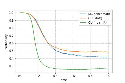
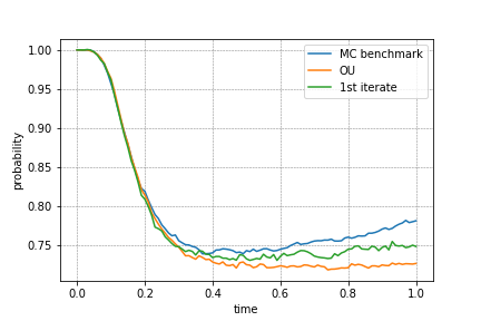
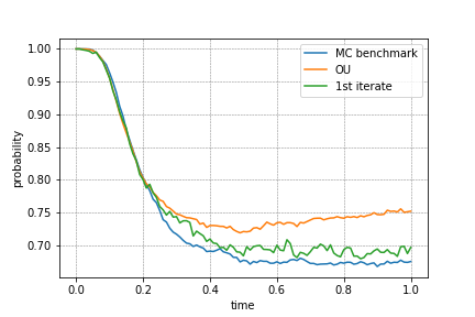
and Of course, is computed numerically. Note that (63) is the deterministic counterpart of the semilinear SDE (18), and that the expected value function of the OU process coincides with in the interval by the choice of . The intuition is that, at least when the noise is weak, the trajectories of the semilinear solutions are “close” to allowing the th iterate to perform better than it would do with . Figure 1 clearly displays this idea in the case of (bounded) cubic nonlinearity treated below (see (64)). Furthermore, in the sequel we monitor the effect of the time–shift on the first order approximation provided by our scheme. All the simulations are carried out using the High Performance Computing Center of the Scuola Normale Superiore (https://hpccenter.sns.it).
We work in dimension , with for some , and we denote by the vector with all components equal to . In particular, given , we are interested in applying our iterates to approximate , whose reference value is computed by averaging samples of obtained by the Euler–Maruyama scheme with time step . The same strategy is used to obtain the th iterate . In order to calculate the numerical integrals appearing in the formulas for (see (49)-(17)), we use left Riemann sums in a uniform grid with mesh We will keep track of the relative error , defined by
Finally, we will mainly focus on the first iteration, with the aim of understanding the possible improvements that it provides over the linear approximation of the OU process. In fact, although it is possible to implement our scheme up to any order thanks to (17), one needs an dimensional integral (in time) to get the iterate fact which complicates the application of our method and may result in losing its computational advantage over the classical Euler–Maruyama approach. In what follows, we fix the initial time and the threshold . For the subordinator , we set in (3).
We first take . Table 2 shows the performance of the first order approximation of the iterative scheme with time–shift as varies in , and . Table 2 is analogous, but it refers to (no time–shift). The first thing we notice is that in both cases the first iteration improves on the outcomes of the linear approximation. The role of the time–shift is evident in the column : it allows to be closer to the benchmark probability, and the first iterate builds on this to guarantee a better overall performance, particularly when is close to .
| 0.55 | 0.687 | 0.639 | 6.99e-2 | 0.012 | 5.24e-2 |
| 0.65 | 0.713 | 0.676 | 5.19e-2 | 1.34e-2 | 3.31e-2 |
| 0.75 | 0.794 | 0.737 | 7.18e-2 | 3.34e-2 | 2.97e-2 |
| 0.85 | 0.899 | 0.863 | 0.040 | 1.87e-2 | 1.92e-2 |
| 0.55 | 0.691 | 0.502 | 0.274 | 0.101 | 0.127 |
| 0.65 | 0.720 | 0.558 | 0.225 | 0.110 | 7.22e-2 |
| 0.75 | 0.785 | 0.666 | 0.151 | 8.84e-2 | 0.039 |
| 0.85 | 0.896 | 0.840 | 6.25e-2 | 3.86e-2 | 1.94e-2 |
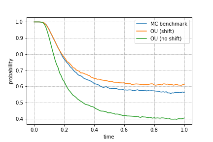
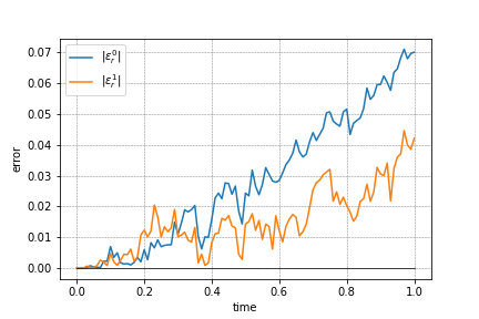
Next, Figure 2 displays the behavior in time –up to – of the first order approximation in the case of time–shift for two strengths of noise ( and ). Here is fixed. The panels of this figure highlight the benefits of considering over the starting OU estimates, especially when the noise is weak.
Secondly, we analyze the polynomial vector field
| (64) |
where and , with ()
The maps are smooth approximations of the maximum function and replace the infinity norm in (64), allowing coherently with our theoretical framework. Therefore is to be interpreted as a cubic nonlinearity with a cutoff for large values of For our experiments, we consider and . In Tables 4-4 we report the outcomes of simulations with and without , respectively, when and varies in In particular, Table 4 shows that, in the case of time–shift, the first iterate always remarkably outperforms the linear approximation. On the contrary, when (Table 4), deteriorates the OU estimate, and we are forced to implement the second iterate to get an accuracy similar to the one provided by the time–shift (compare the columns , Table 4, and , Table 4). Of course, the trade–off in the introduction of consists in substantially increasing the computational time.
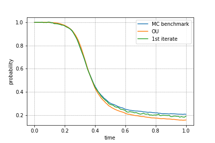
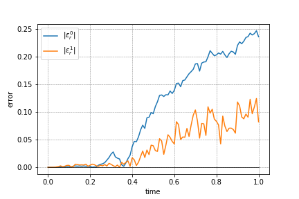
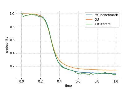
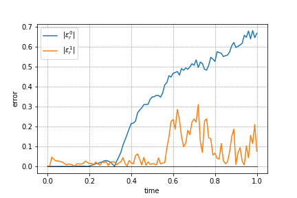
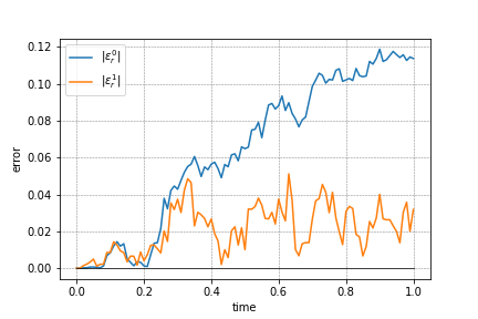
Finally, in Figure 3 we investigate the trajectories of and of the first order approximation in the time interval , as well as the corresponding absolute relative errors. Here we fix and consider two strengths of noise: and . As already observed in the sine case, the advantages in introducing the first iterate are rather evident. Overall, we conclude that proves to be a versatile and computationally cheap method to improve on the performances of the linear approximation.
| 0.55 | 0.501 | 0.562 | -0.122 | -5.19e-2 | -1.82e-2 |
| 0.65 | 0.531 | 0.594 | -0.119 | -6.65e-2 | 6.59e-3 |
| 0.75 | 0.587 | 0.648 | -0.104 | -6.40e-2 | 5.11e-3 |
| 0.85 | 0.679 | 0.743 | -9.43e-2 | -7.95e-2 | 2.28e-2 |
| 0.55 | 0.495 | 0.374 | 0.244 | -9.64e-4 | 0.246 | 0.109 | 2.62e-2 |
| 0.65 | 0.536 | 0.396 | 0.261 | -2.74e-2 | 0.312 | 0.142 | 4.74e-2 |
| 0.75 | 0.586 | 0.462 | 0.212 | -8.16e-2 | 0.351 | 0.191 | 2.49e-2 |
| 0.85 | 0.680 | 0.608 | 0.106 | -8.20e-2 | 0.226 | 0.138 | 2.35e-2 |
Appendix A Proof of Lemma 4
Proof of Lemma 4
Let us fix and a direction ; note that all the assertions of the statement are true for by construction of the stochastic flow, hence we only focus on . For every and define the incremental ratio function
| (65) |
Notice that, for every (omitting to keep notation short)
where we recall that . Thus, an application of Gronwall’s lemma shows that for all and . Next, taking and we compute from (A)
| (66) |
where . Therefore another application of Gronwall’s lemma shows that the mapping is Lip–continuous in uniformly in , and by the theorem of extension of uniformly continuous functions we obtain the existence of . Now by dominated convergence we are allowed to pass to the limit in (A), which yields
| (67) |
Given the arbitrarity of , this equation shows that the mapping belongs to with .
In order to analyze higher–order derivatives, we work by induction; fix and suppose as inductive hypothesis that , with the estimate in (19) holding true for a sum from to . Moreover, assume that for every multi–index with length one has, for any (omitting )
| (68) |
Here is the canonical basis of and with denoting a sum of products where one factor is a (partial) derivative at of up to order and the others are (partial) derivatives at of up to order . In particular, when (cfr. (67)). At this point, consider and fix a multi–index with length ; by analogy with (A), for any and define the incremental ratio function
Note that for any we can write (, )
and that, further, the inductive hypothesis of boundedness for the derivatives of (see (19)), together with the structure of and ensures that
for some constant . These facts, the Lip–continuity of the map in uniformly in and computations analogous to those in (A) entail that there exists . The arbitrarity of and coupled with Gronwall’s lemma provides us with the desired bound (19) for the derivatives of order , and finally by dominated convergence the validity of (68) for a multi–index of length is a consequence of the chain rule. In particular, . The proof is then complete, considering that the base case is provided by (67).
References
- [1] Beck, C., Becker, S., Grohs, P., Jaafari, N., & Jentzen, A. (2021). Solving the Kolmogorov PDE by means of deep learning. Journal of Scientific Computing, 88(3), 1–28.
- [2] Benth, F. E., Benth, J. S., & Koekebakker, S. (2008). Stochastic modelling of electricity and related markets (Vol. 11). World Scientific.
- [3] Bogachev, V. I. (2007). Measure theory (Vol. 1). Springer Science & Business Media.
- [4] Bogdan, K., Stós, A., & Sztonyk, P. (2003). Harnack inequality for stable processes on d-sets. Studia Math, 158(2), 163–198.
- [5] Bondi, A. (2022). Smoothing effect and Derivative formulas for Ornstein–Uhlenbeck processes driven by subordinated cylindrical Brownian noises. Journal of Functional Analysis, 283(10), 109660.
- [6] Da Prato, G. (2014). Introduction to stochastic analysis and Malliavin calculus (Vol. 13). Springer.
- [7] Da Prato, G., & Zabczyk, J. (1996). Ergodicity for infinite dimensional systems (Vol. 229). Cambridge University Press.
- [8] Da Prato, G., & Zabczyk, J. (2014). Stochastic equations in infinite dimensions. Cambridge University Press.
- [9] Flandoli, F., Luo, D., & Ricci, C. (2021). A numerical approach to Kolmogorov equation in high dimension based on Gaussian analysis. Journal of Mathematical Analysis and Applications, 493(1), 124505.
- [10] Flandoli, F., Luo, D., & Ricci, C. (2023). Numerical computation of probabilities for nonlinear SDEs in high dimension using Kolmogorov equation. Applied Mathematics and Computation, 436, 127520.
- [11] Jacod, J. (2006). Calcul stochastique et problemes de martingales (Vol. 714). Springer.
- [12] Jacod, J., & Shiryaev, A. (2013). Limit theorems for stochastic processes (Vol. 288). Springer Science & Business Media.
- [13] Kallenberg, O. (1997). Foundations of modern probability (Vol. 2). New York: Springer.
- [14] Karatzas, I., & Shreve, S. E. (1998). Brownian motion. In Brownian Motion and Stochastic Calculus (pp. 47–127). Springer, New York, NY.
- [15] Kunita, H. (2019). Stochastic Flows and Jump–Diffusions (Vol. 92). Springer.
- [16] Marinelli, C., & Röckner, M. (2014). On maximal inequalities for purely discontinuous martingales in infinite dimensions. In Séminaire de Probabilités XLVI (pp. 293–315). Springer, Cham.
- [17] Priola, E. (2018). Davie’s type uniqueness for a class of SDEs with jumps. In Annales de l’Institut Henri Poincaré, Probabilités et Statistiques (Vol. 54, No. 2, pp. 694–725). Institut Henri Poincaré.
- [18] Priola, E. (2020). On Davie’s uniqueness for some degenerate SDEs. Theory of Probability and Mathematical Statistics, 103, 41–58.
- [19] Priola, E., & Zabczyk, J. (2011). Structural properties of semilinear SPDEs driven by cylindrical stable processes. Probability theory and related fields, 149(1-2), 97–137.
- [20] Sato, K.-I. (1999). Lévy processes and infinitely divisible distributions. Cambridge University Press.
- [21] Wang, F. Y., Xu, L., & Zhang, X. (2015). Gradient estimates for SDEs driven by multiplicative Lévy noise. Journal of Functional Analysis, 269(10), 3195–3219.
- [22] Zhang, X. (2013). Derivative formulas and gradient estimates for SDEs driven by -stable processes. Stochastic Processes and their Applications, 123(4), 1213–1228.