CLAD: A Contrastive Learning based Approach for Background Debiasing

Abstract

Convolutional neural networks (CNNs) have achieved superhuman performance in multiple vision tasks, especially image classification. However, unlike humans, CNNs leverage spurious features, such as background information to make decisions. This tendency creates different problems in terms of robustness or weak generalization performance. Through our work, we introduce a contrastive learning-based approach (CLAD) to mitigate the background bias in CNNs. CLAD encourages semantic focus on object foregrounds and penalizes learning features from irrelavant backgrounds. Our method also introduces an efficient way of sampling negative samples. We achieve state-of-the-art results on the Background Challenge dataset, outperforming the previous benchmark with a margin of 4.1%. Our paper shows how CLAD serves as a proof of concept for debiasing of spurious features, such as background and texture (in supplementary material).

1 Introduction

CNNs have achieved superhuman performance on various computer vision tasks such as segmentation [Wei et al.(2022)Wei, Hu, Xie, Zhang, Cao, Bao, Chen, and Guo], classification [Voulodimos et al.(2018)Voulodimos, Doulamis, Doulamis, and Protopapadakis, He et al.(2016)He, Zhang, Ren, and Sun, Benz et al.(2021)Benz, Ham, Zhang, Karjauv, and Kweon], object detection[Zhang et al.(2022)Zhang, Li, Liu, Zhang, Su, Zhu, Ni, and Shum], etc. However, it has been observed that CNNs have a different understanding of images in contrast to humans [Geirhos et al.(2017)Geirhos, Janssen, Schütt, Rauber, Bethge, and Wichmann]. Specifically, in the case of classification, it has been observed that CNNs can be biased towards the background information instead of the foreground object [Zhu et al.(2017)Zhu, Xie, and Yuille, Barbu et al.(2019)Barbu, Mayo, Alverio, Luo, Wang, Gutfreund, Tenenbaum, and Katz, Beery et al.(2018)Beery, Van Horn, and Perona, Xiao et al.(2020)Xiao, Engstrom, Ilyas, and Madry, Sehwag et al.(2020)Sehwag, Oak, Chiang, and Mittal], high-frequency components [Yin et al.(2019)Yin, Gontijo Lopes, Shlens, Cubuk, and Gilmer, Ortiz-Jimenez et al.(2020)Ortiz-Jimenez, Modas, Moosavi, and Frossard, Machiraju et al.(2022)Machiraju, Choung, Herzog, and Frossard], and textures rather than shapes [Geirhos et al.(2019)Geirhos, Rubisch, Michaelis, Bethge, Wichmann, and Brendel, Islam et al.(2021)Islam, Kowal, Esser, Jia, Ommer, Derpanis, and Bruce]. In particular, Kai et al.[Xiao et al.(2020)Xiao, Engstrom, Ilyas, and Madry] showed that CNNs tend to correlate class labels heavily with background information. Further, they showed that, when the foreground object is removed, CNNs still perform surprisingly well solely in the presence of the background of the image. The authors created the Background Challenge [Xiao et al.(2020)Xiao, Engstrom, Ilyas, and Madry] which measures models’ robustness to various changes the background. They further showed that most state-of-the-art image classification models exhibit a poor generalization ability in this challenge due to large background bias. These biases lead to an over-dependence of the model on irrelevant/spurious features. Further, such biases can be exploited to fool the classifiers by simply altering the background of the object [Moayeri et al.(2022)Moayeri, Pope, Balaji, and Feizi] or adding different textures to the image [Geirhos et al.(2019)Geirhos, Rubisch, Michaelis, Bethge, Wichmann, and Brendel].

To mitigate such biases, conventional data augmentation is often used, wherein the model is exposed to additional training data, in order to decorrelate the spurious features and the class label. However, to completely eliminate bias and prevent memorization (overfitting) of data, the model usually requires a very large amount of data for augmentation. Also, previous works [Wang et al.(2019b)Wang, Zhao, Yatskar, Chang, and Ordonez, Zhao and Gordon(2019)] have shown that conventional data augmentation is insufficient to discard spurious features and remains susceptible to small changes. Therefore, an effective data augmentation method has to be applied to ensure that the best features are extracted during training while introducing minimal computational overhead.

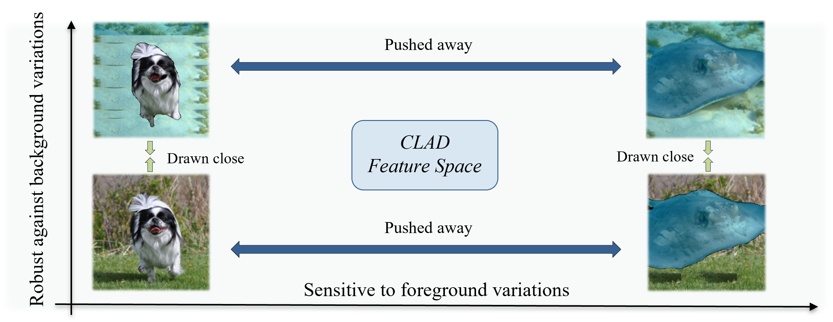
Figure 1: CLAD learns feature space which is robust against background variations and sensitive to foreground features.

Here, we propose a Contrastive Learning based Approach for background Debiasing (CLAD) model, where contrastive learning (CL) is introduced to mitigate the biases more effectively. In contrastive learning, for each data point (anchor), both positive samples (sharing anchor’s distribution) and negative samples (carries different information as anchor) are generated. Then, CL minimizes the distances between the anchor and positive samples and maximizes the distances between the anchor and negative samples in feature space. To this end, in the latent embedding, attributes that belong to the same distribution (relevant features, e.g., foregrounds) are aggregated together, while unwanted biases (e.g., backgrounds) are separated from the anchor. Hence, our method, CLAD, uses contrastive learning to learn a background-robust feature space, by carefully constructing the positive and negative samples. Positive samples are generated by changing the anchor’s background. The negative samples, on the other hand, contain distinctive foreground information but similar background as the anchor (Fig. 2). Moreover, instead of generating negative samples, we introduce a novel mechanism to sample negative samples without introducing extra costs, where we sample negative pairs during the training process from generated positive samples while ensuring the sampled negative samples share similar background information as anchor. Thus, our novel method allows for both the scalability of negative samples as well as having similar background as anchor.
We show that, our CLAD model outperforms the state-of-the-art methods on the Background Challenge dataset [Xiao et al.(2020)Xiao, Engstrom, Ilyas, and Madry], while it has almost no accuracy drop on original images. It samples negative samples effectively without introducing heavy computational costs. Especially, CLAD outperforms on the random-background dataset (Mixed-Rand) by a margin of $4.1\%$, while all the other state-of-the-art methods showed a major performance drop. We also show that CLAD can be applied to mitigate the influence of other discriminative features apart from background, like object texture (in supplementary material), while improving model’s shape bias.

2 Related Work

Feature biases are thought to happen because of the data memorization (overfitting) and are exacerbated when training the over-parameterized models [Khani and Liang(2021)]. One effective way to mitigate these problems is to augment with samples emphasizing desirable features instead of irrelevant spurious ones. In background-biased settings, Kai et al.[Xiao et al.(2020)Xiao, Engstrom, Ilyas, and Madry] showed that training models on images with random unrelated backgrounds for a given foreground helped reduce the background bias of the model. However, this also significantly reduced performance on the original dataset (Table 2). Further, as mentioned in the previous section, conventional data augmentation is not optimal for debiasing; hence, we rather look at contrastive learning.

Contrastive Learning (CL) [Hadsell et al.(2006)Hadsell, Chopra, and LeCun] helps learn robust feature spaces that are close across a data distribution and attributes that set apart a data distribution from another. CL has shown great promise in self-supervised regimes [Chen et al.(2020)Chen, Kornblith, Norouzi, and Hinton, He et al.(2020)He, Fan, Wu, Xie, and Girshick, Grill et al.(2020)Grill, Strub, Altché, Tallec, Richemond, Buchatskaya, Doersch, Avila Pires, Guo, Gheshlaghi Azar, et al.] while recently, it has also been applied to the supervised learning domain and achieved promising results [Khosla et al.(2020)Khosla, Teterwak, Wang, Sarna, Tian, Isola, Maschinot, Liu, and Krishnan, Lo et al.(2021)Lo, Chang, Chiu, Huang, Chen, Chang, and Jou, Liu et al.(2021)Liu, Yan, and Alahi]. CL has been used in a self-supervised manner to help debias models [Taghanaki et al.(2021)Taghanaki, Choi, Khasahmadi, and Goyal, Lee et al.(2022)Lee, Hwang, Kang, and Zhang, Ryali et al.(2021)Ryali, Schwab, and Morcos, Mo et al.(2021)Mo, Kang, Sohn, Li, and Shin]. In the fully supervised learning domain, previous works have shown that utilizing contrastive loss as an auxiliary loss can encourage learning more robust features with higher generalization abilities through careful contrastive pair construction [Lo et al.(2021)Lo, Chang, Chiu, Huang, Chen, Chang, and Jou, Liu et al.(2021)Liu, Yan, and Alahi]. To the best of our knowledge, we are the first to leverage contrastive learning as an auxiliary loss to improve the model’s background robustness in a fully-supervised setting.

3 Methodology

In this section, we go through the contrastive learning framework and then introduce our background-debiased contrastive pair sampling strategy, and finally present our overall learning framework.

3.1 Contrastive Learning

We use the popular InfoNCE [Gutmann and Hyvärinen(2010), Oord et al.(2018)Oord, Li, and Vinyals] loss as our contrastive loss term. This loss function can be viewed as an (N+1)-way cross-entropy classification loss to distinguish between one positive sample and N negative samples, and is written as:

$$\mathcal{L}_{con}=-log\left[\frac{e^{s(x,x^{+})/\tau}}{e^{s(x,x^{+})/\tau}+\sum_{i=1}^{N}e^{s(x,x_{i}^{-})/\tau}}\right]$$ (1)

where $s(x_{1},x_{2})=(x_{1}\cdot x_{2})/(\left\|x_{1}\right\|\left\|x_{2}\right\|$) is the cosine similarity function and $\tau$ is the temperature parameter; $x,x^{+},x^{-}_{i}$ represent the feature representations for the anchor, the positive sample and the multiple negative samples, respectively. It brings positive sample pairs closer in the feature space, while it pushes the anchor apart from negative samples.

3.2 Background-debiased Sampling

One crucial contribution of CLAD is an efficient sampling approach for contrastive pairs which are harder to discrminate from the anchor. Conventionally, in contrastive learning, positive samples are obtained by applying a combination of different data augmentations to the anchor. Negative samples, on the other hand, come from views of other images (see Fig. 2 (a)). However, such sampling of contrastive pairs would lead to poor robustness on backgrounds due to two reasons: 1) increasing feature similarity between positive pairs would simultaneously encourage background bias due to their shared background information; 2) likewise, as negative samples carry different background information compared to the anchor, minimizing feature similarity between negative pairs would increase the model’s sensitivity to background variations.

These problems are solved in CLAD’s background-debiased contrastive pair sampling approach, where background information is no longer shared between positive pairs, and negative pairs share similar background information, as shown in Fig. 2 (b). The contrastive pairs are created as follows:

Positive Samples are created by replacing the background of the anchor with a different-class background (chosen randomly). Following the method in Background Challenge dataset [Xiao et al.(2020)Xiao, Engstrom, Ilyas, and Madry], we use GrabCut [Rother et al.(2004)Rother, Kolmogorov, and Blake] to separate the foreground and background of a given anchor image (see supplementary material for details). The foreground of the anchor is then placed in a background found in another random class (other than the anchor class).

Negative Sample It is crucial to have a large number of negative samples in contrastive learning [Chen et al.(2020)Chen, Kornblith, Norouzi, and Hinton, He et al.(2020)He, Fan, Wu, Xie, and Girshick]. However, using the same method to create positive samples, i.e., replacing the foreground of the anchor image instead and keeping the background, needs to be repeated many times to create multiple negative samples. This leads to a high computational cost which linearly scales the cost per batch by the number of negative samples. To solve this issue, we introduce a negative sample dictionary.

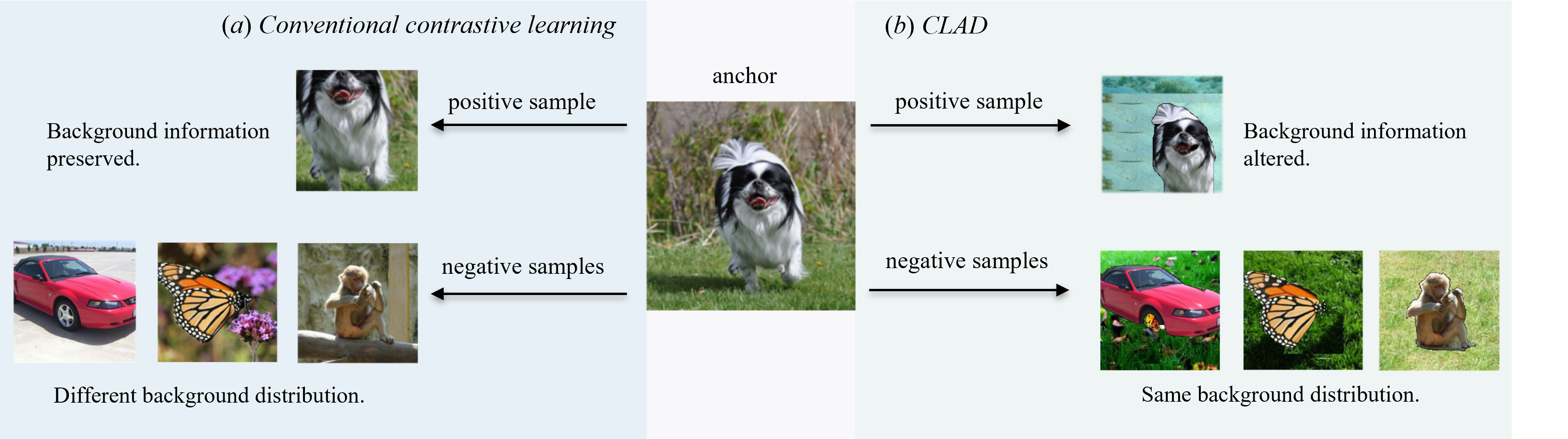
Figure 2: Contrastive pair sampling strategies, (a) used in conventional contrastive learning, (b) CLAD’s background-debiased sampling strategy

We define our negative sample dictionary as a dictionary with queues for each class, containing the latent representation for each negative sample. Each queue, has samples whose background belongs to the class represented by the queue. The size of each queue is the same as the number of negative samples (N). In each batch, we use the generated positive samples to update the queue. The old samples are dequeued (deleted) when new samples are enqueued (added) to the queue following a first in, first out order. Therefore, the negative samples are reused until they get replaced in the queue.

This differs from the commonly used memory bank [He et al.(2020)He, Fan, Wu, Xie, and Girshick] for storing negative samples in two ways:

• It only stores features for background-augmented images where the foreground and background classes are decoupled.

• As a dictionary, it contains keys for background labels of the stored samples. Samples are stored in the queue whose key corresponds to their background labels.

We illustrate the mechanism in Fig. 3. The dictionary contains the keys of the background label, and we show two examples in the Figure. In the example for updating the dictionary with generated samples, the sample has a background of Fish class, so it will enter the queue within the Fish key (the foreground label is ignored in this process). The other example shows the sampling process for negative samples from the dictionary: the anchor is an image from Dog class; hence we draw all samples in the queue within the Dog key in the dictionary.

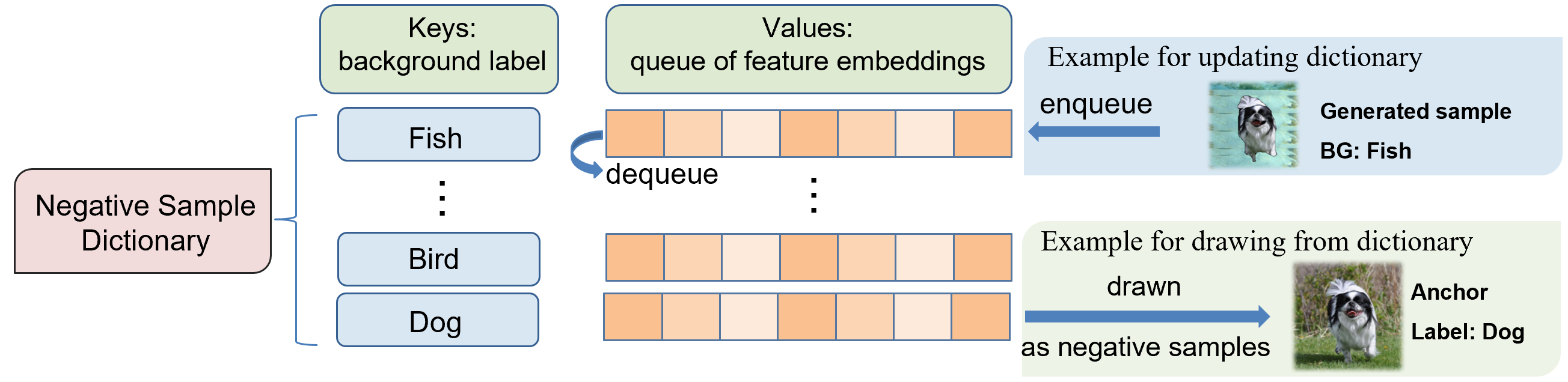
Figure 3: Illustration of using dictionary to store negative sample candidates.

Using the negative sample dictionary guarantees that similar background information is shared between negative pairs simultaneously. Hence, our method provides a memory-efficient way of scaling negative samples.

3.3 Training Objective

The overall loss function is composed of two terms: the conventional supervised classification loss (for learning distinguishable features) and contrastive loss (for improving background robustness). After we generate positive and negative sample pairs (as described in Sec 3.2), we calculate the contrastive loss using the InfoNCE loss function. To enforce the correct classification of the positive samples, we can optionally include a classification loss for such samples and refer to the model with this additional loss term as CLAD+. For the supervised classification loss, we use the conventional cross-entropy loss. Specifically,

the overall loss for CLAD can be written as:

$$\mathcal{L}_{CLAD}=\mathcal{L}_{class}(x)+\lambda*\mathcal{L}_{con}(x,x^{+},x^{-})$$ (2)

For CLAD+, the loss is written as:

$$\mathcal{L}_{CLAD+}=\mathcal{L}_{class}(x)+\mathcal{L}_{class}(x^{+})+\lambda*\mathcal{L}_{con}(x,x^{+},x^{-})$$ (3)

Here, $\lambda$ is a hyperparameter for the weight that controls the importance of the contrastive term $\mathcal{L}_{con}$. Its magnitude controls the degree of background robustness learned by the model.

3.4 Training

As illustrated in Fig. 4, for each batch, we generate positive samples. Then, the generated positive samples are used to update the negative sample dictionary. The classification loss is calculated for the anchor (and also for the positive sample for CLAD+). When calculating the contrastive loss, the negative samples are drawn accordingly from the negative sample dictionary based on the label of each anchor. The contrastive loss is finally calculated based on feature representations for the anchors, positive and negative samples.

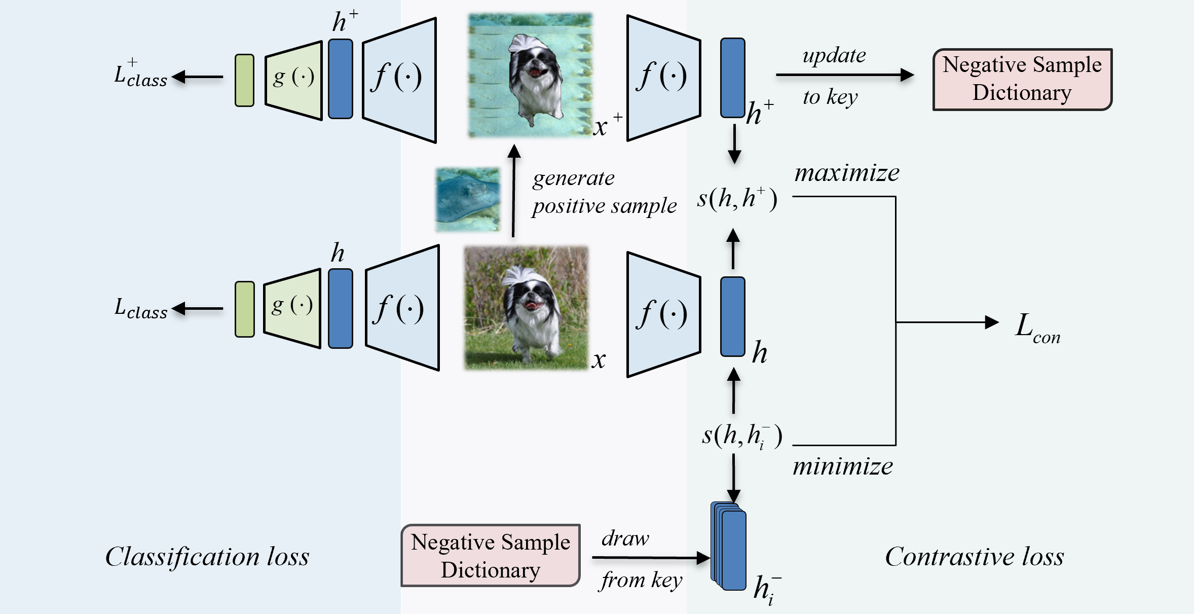
Figure 4: Illustration of the proposed supervised learning with contrastive learning approach.

4 Experiment

In this section, we present the results for CLAD and CLAD+ on the Background Challenge dataset [Xiao et al.(2020)Xiao, Engstrom, Ilyas, and Madry].

4.1 Challenge Description

Kai et al.[Xiao et al.(2020)Xiao, Engstrom, Ilyas, and Madry] initiated the Background Challenge [Xiao et al.(2020)Xiao, Engstrom, Ilyas, and Madry] dataset in 2020. The dataset aggregates a subset of images in ImageNet based on WordNet hierarchy [Miller(1995)] into 9 classes, creating the ImageNet-$9$ dataset. Several variations are made on the images’ background or foreground in original ImageNet-$9$, as summarized in Table 1.

Dataset	Foreground	Background	Summary
Original	Original	Original	Original unaltered images
Only-FG	Original	None (Black)	Images with only the foreground (background removed)
Only-BG-T	None	Original	Images with only the background
Mixed-Rand	Original	Completely Random	Images with a random background
Mixed-Same	Original	Random-same-class	Images with a background from the same class

Table 1: Description of the variations of ImageNet-$9$[Xiao et al.(2020)Xiao, Engstrom, Ilyas, and Madry]

The goal of the Background Challenge is to achieve high accuracy on the Mixed-Rand dataset, where the background class is selected randomly and provides no information on image label. Intuitively, models with high background bias would suffer from low accuracy on this dataset. Additionally, the challenge also defines a metric to quantify the background bias: BG-Gap, which is defined as the accuracy gap between the Mixed-Same and Mixed-Rand datasets. The BG-Gap represents the performance drop due to background class signal change [Xiao et al.(2020)Xiao, Engstrom, Ilyas, and Madry], or more intuitively, how much accuracy is actually gained by background bias.

4.2 Experimental Settings

We adopt a ImageNet-pretrained ResNet-50 as our backbone [Xiao et al.(2020)Xiao, Engstrom, Ilyas, and Madry]. Adam [Kingma and Ba(2015)] is used as the optimizer with default settings ($\beta_{1}=0.9$ and $\beta_{2}=0.999$) and no weight decay is used. The total number of training epochs is 60, and the batch size is 64. The learning rate is set to be $1e^{-3}$ and decays to $1e^{-4}$ after 20 epochs. After trial and error, the hyperparameter $\lambda$ for the weight of the contrastive loss is set to $1$ (ablation in 4.4) and the temperature parameter $\tau$ is set to 0.2. Data augmentations, including Random Resized Crop, Random Horizontal Flip, and Color Jitter, are used in our experiments. Note that for the generated positive samples, these conventional data augmentations are applied after the background augmentation. For each anchor, we construct one positive sample and draw 32 negative samples (details in supplementary material) from the negative sample dictionary. In this section, we evaluate the performance of CLAD on the Background Challenge dataset. For comparison, we compare the performance of CLAD to three baselines, which are trained in conventional, fully supervised settings, which include:

• Base(IN) ImageNet-trained ResNet-50 with prediction mapped to ImageNet-$9$.

• Base(IN9) ResNet-50 trained on Original with a fully supervised setting.

• Base(MR) ResNet-50 trained on Mixed-Rand with a fully supervised setting.

In addition we also compare to previous works on Background challenge dataset, the results of which are presented in Table 2.

4.3 Accuracy

CLAD and CLAD+ do not suffer any accuracy trade-off on the Original dataset compared to the baseline models (0.4% and 0.1% drop correspondingly).

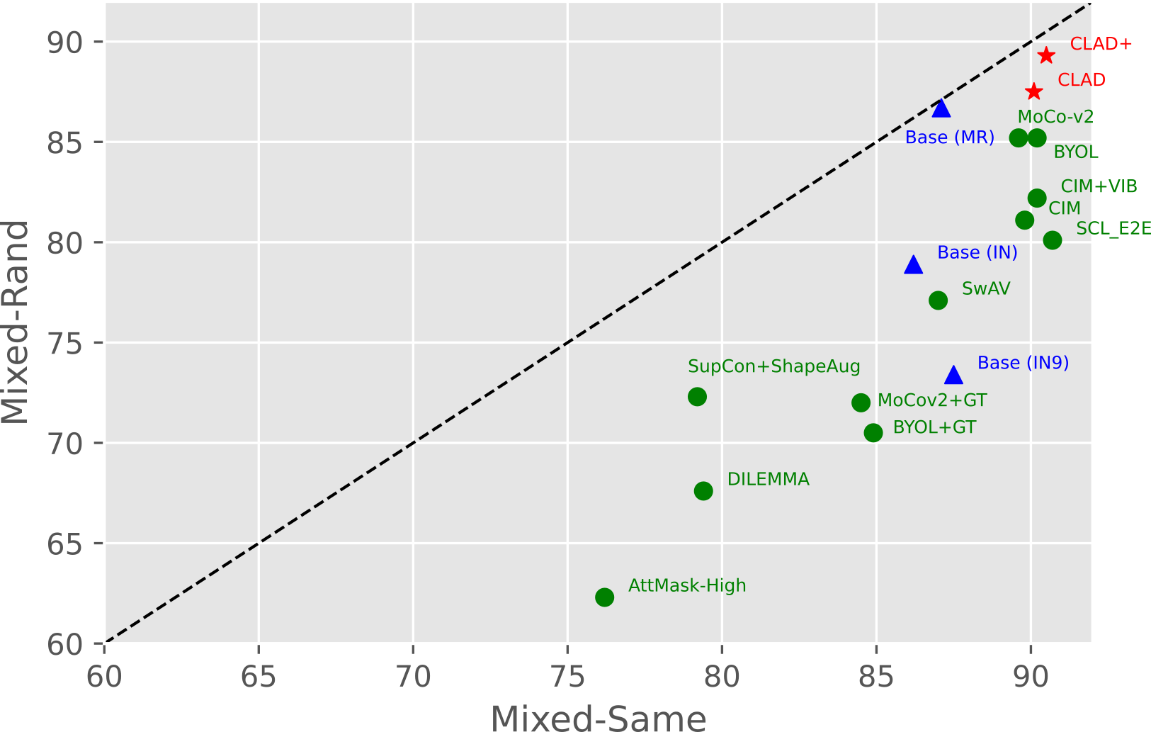
Figure 5: Model performances on Mixed-Same (x-axis) and Mixed-Rand (y-axis) data. Models closer to the Identity dashed line has lower background bias.

Our method outperforms all previous benchmarks by a large margin (4.1% for CLAD+ and 2.3% for CLAD) on Mixed-Rand dataset, which is the most important indicator for the model’s generalization ability to varying-background images.

It is possible to have a very small BG-GAP as well as very low accuracy on both the Mixed-Same and Mixed-Rand datasets. However, that would not be reflective of the background bias or generalization ability of the model. Hence, we need high performance on both datasets along with a smaller gap between them, to have less background bias. We plot the accuracies of these datasets in Fig. 5, wherein models that lie closer to the identity line have lower background bias. Additionally, the further right from the model’s line, the higher its bias. We can see from the Figure that our models CLAD and CLAD+ have the best performance among all the models.

Type	Model	Original $\uparrow$	Only-FG $\uparrow$	Mixed-Rand $\uparrow$	Mixed-Same $\uparrow$	Only-BG-T $\downarrow$	BG-Gap $\downarrow$
Baselines	Base (IN) [Xiao et al.(2020)Xiao, Engstrom, Ilyas, and Madry]	96.2	-	76.3	82.3	17.8	6.0
	Base (IN9)	96.0	86.0	73.4	87.5	42.9	14.1
	Base (MR)	88.4	89.5	86.7	87.1	12.8	0.4
Others	CIM [Taghanaki et al.(2021)Taghanaki, Choi, Khasahmadi, and Goyal]	97.7	-	81.1	89.8	-	8.8
	SCL_E2E [Taghanaki et al.(2021)Taghanaki, Choi, Khasahmadi, and Goyal]	98.2	-	80.1	90.7	-	10.6
	CIM+VIB [Taghanaki et al.(2021)Taghanaki, Choi, Khasahmadi, and Goyal]	97.9	-	82.2	90.2	-	8.0
	SupCon+ShapeAug[Lee et al.(2022)Lee, Hwang, Kang, and Zhang]	-	-	72.3	79.2	-	6.89
	MoCo-v2 (BG Swaps)[Ryali et al.(2021)Ryali, Schwab, and Morcos]	95.2	87.5	85.2	89.6	11.4	4.4
	BYOL (BG Random)[Ryali et al.(2021)Ryali, Schwab, and Morcos]	96.1	88.3	85.2	90.2	12.9	5.0
	SwAV (BG RM)[Ryali et al.(2021)Ryali, Schwab, and Morcos]	95.3	86.8	77.1	87.0	18.2	9.9
	AttMask-High[Kakogeorgiou et al.(2022)Kakogeorgiou, Gidaris, Psomas, Avrithis, Bursuc, Karantzalos, and Komodakis]	89.8	75.2	62.3	76.2	15.3	9.9
	MoCov2+GT[Mo et al.(2021)Mo, Kang, Sohn, Li, and Shin]	89.7	72,7	72.0	84.5	40.1	12.5
	BYOL+GT[Mo et al.(2021)Mo, Kang, Sohn, Li, and Shin]	91.0	72.6	70.5	84.9	41.2	14.4
	DILEMMA[Sameni et al.(2022)Sameni, Jenni, and Favaro]	91.8	77.8	67.6	79.4	9.3	10.2
Ours	CLAD+	95.6	94.6	89.3	90.5	22.6	1.2
	CLAD	95.9	93.8	87.5	90.1	31.3	2.6

Table 2: Accuracy ($\%$) comparison between CLAD, CLAD+ against baselines and benchmarks on the Background Challenge. ‘-’ represents value missing in the references. Note that the models in this table are trained with different sizes of dataset and level of supervision, in this case the BG-Gap is the fairest comparison across all models indicating background bias.

4.4 Analysis

Feature Consistency We estimate the percentage of encoded foreground information by calculating the features’ cosine similarity between image pairs sharing the same foreground. This metric can also be intuitively reflect as how much of the features are extracted from the foreground. We also define a more direct metric, decision consistency, which summarizes the fraction of consistent decisions after background change. This can be expressed as $\frac{1}{N}\sum_{i=1}^{N}\mathbbm{1}(\operatorname*{arg\,max}g(x_{i})=\operatorname*{arg\,max}g(\hat{x}_{i}))$, where, $g(.)$ is the classifier, $(x_{i},\hat{x}_{i})$ represent image pairs with same foreground but different background. The higher the decision consistency, the smaller the effect of background changes on the models’ decisions. For details, see Table 3.

Model	Feature Similarity	Decision Consistency
Base (IN9)	0.795	0.800
Base (MR)	0.864	0.864
CLAD+	0.920	0.969
CLAD	0.914	0.915

Table 3: Feature similarity and decision consistency between Original and Mixed-Rand datasets. CLAD and CLAD+ can extract features over 90% similar to the extracted features before background variation, meaning that a large amount of the features they learned from the original images are from the foreground, well explaining their performance on the background challenge dataset.

Interpretability: Saliency map provides intuitive illustration for models’ areas of focus in images. Fig. 6 illustrates the SmoothGrad[Smilkov et al.(2017)Smilkov, Thorat, Kim, Viégas, and Wattenberg] saliency maps of the CLAD and CLAD+, compared with two baseline models. It shows that the saliency maps for CLAD+ and CLAD focus more on the foreground object with a much cleaner saliency map than Base(IN9) and even Base(MR). An interesting observation is that, the saliency map of Base(IN9) and Base(MR) on the wolf image (second row) shows these baseline models rely on background snow for identifying wolf, which is a well-known example for CNN’s background bias [Szegedy et al.(2015)Szegedy, Liu, Jia, Sermanet, Reed, Anguelov, Erhan, Vanhoucke, and Rabinovich]. CLAD+ and CLAD are able to identify wolf while ignoring background snow, relatively better than base models.

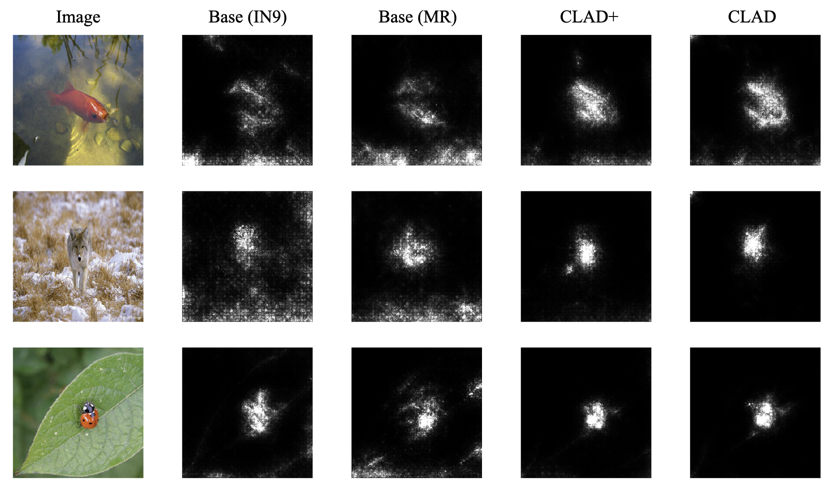
Figure 6: Saliency maps of CLAD+ and CLAD, compared with two baseline models.

Importance of Contrastive Loss: The hyper-parameter $\lambda$ is the weight of the contrastive loss term in our overall loss function. In Fig. 7 we show that the magnitude of $\lambda$ determines the background robustness of the CLAD model. This Figure presents the varying accuracy on Mixed-Rand dataset, as well as Original ImageNet-$9$, with increasing $\lambda$. The CLAD models do not have any performance deterioration when the contrastive loss is introduced with equal weight as the classification loss. Its performance on Original dataset remains the same while increasing on Mixed-Rand. However, if the value of $\lambda$ is further increased, i.e., the contrastive loss becomes more important than the supervised losses ($\lambda>1$), then there is a performance deterioration. This indicates that we need a balanced mix of both supervised and contrastive losses for ideal performance.

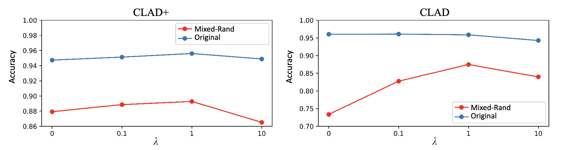
Figure 7: Accuracy on Mixed-Rand dataset and Original ImageNet-$9$ with respect to different values of $\lambda$

5 Conclusion

Through our work, we present a novel contrastive learning-based approach for background debiasing called CLAD. It samples background-debiased contrastive pairs efficiently. Our work showcases state-of-the-art performance on the Background Challenge dataset. We also show an analysis of our model’s features, which explain its superior performance compared to the standard trained model. Further, we empirically demonstrate the need for proper balance between contrastive and supervised losses for the effective debiasing of the model. As a result, training with the proposed contrastive learning method reduces the importance of image background and texture information in the decision-making process of CNN models. Theoretically, this approach works for any discriminative feature pairs, and we took foreground vs. background and shape vs. texture (in supplementary material) as an example. In future works, we could further investigate how to extend this approach to other pairs of discriminative features and hopefully guide the CNNs to make decisions based on similar features as humans, thereby improving generalization ability.

Supplementary

I Effect of Negative Sample Dictionary

I.1 Ablation for Negative Sample Dictionary

To validate the effectiveness of negative sample dictionary, we conduct an ablation study. We originally create negative samples, which contain background associated with the anchor’s foreground class. However, for this ablation, we create trivial negative samples, which contain background from random classes and are not necessarily matched with anchor’s foreground class. These trivial negative samples are shared across all anchors.

Table 4 presents the performance comparison between CLAD and CLAD+ models, with their respective counterparts where trivial negative samples are used, denoted as CLAD (Trivial) and CLAD+ (Trivial).

Model	Original$\uparrow$	Only-FG$\uparrow$	Mixed-Rand$\uparrow$	Mixed-Same$\uparrow$	Only-BG-T$\downarrow$	BG-Gap$\downarrow$
CLAD	95.9	93.8	87.5	90.1	31.3	2.6
CLAD (Trivial)	95.5	93.0	85.3	88.9	37.2	3.6
CLAD+	95.6	94.6	89.3	90.5	22.6	1.2
CLAD+ (Trivial)	95.4	94.7	89.1	90.3	24.7	1.2

Table 4: Accuracy ($\%$) comparison between CLAD, CLAD+ against their counterparts where trivial negative samples are used.

We observe that both CLAD and CLAD+ indeed perform better than their counterparts which use trivial negative samples.

I.2 Effect of Different Number of Negative Samples

In Fig. 8, we show the accuracy of using different queue sizes (which is also the number of negative samples) for the dictionary. We choose the size to be 32 as it is the best trade-off for both models.

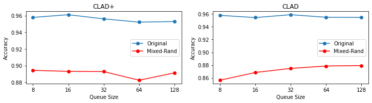
Figure 8: Ablation for the size of the queue in negative sample dictionary. Small queue sizes suffer from insufficient negative samples while large queue size suffers from deterioration of Original accuracy and increased computational costs.

II Foreground Segmentation and Scalability

In our experiments, following the Background Challenge dataset, we used 10 iterations of GrabCut [Rother et al.(2004)Rother, Kolmogorov, and Blake] to segment the images’ foreground using bounding box(bb) information. Instead of Grabcut which relies on bb, we tested using pre-trained U2-Net [Qin et al.(2020)Qin, Zhang, Huang, Dehghan, Zaiane, and Jagersand] to segment the foreground (Results in Table 5). We can see that the accuracy gap between the two methods on the Original and Mixed-Rand dataset is within 1%, and results with U2-Net still beat all previous benchmarks on the Background Challenge. Since the performance does not change significantly, we can replace GrabCut with scalable methods like U2-Net, hence improving the scalability of our method.

In previous works in Table 2 of the main paper, [Lee et al.(2022)Lee, Hwang, Kang, and Zhang, Ryali et al.(2021)Ryali, Schwab, and Morcos] also use foreground segmentation supervision, making them fair comparisons to ours.

Model	FG segmentation	Original $\uparrow$	Mixed-Rand $\uparrow$
Base (IN9)	-	96.0	73.4
CLAD+	GrabCut	95.6	89.3
	U2-Net	96.0	88.3
CLAD	GrabCut	95.9	87.5
	U2-Net	95.8	87.1

Table 5: Accuracy ($\%$) comparison for using GrabCut and U2-Net as foreground segmentation methods.

III Potential Foreground Positional Bias

The Background Challenge dataset may have centered foreground bias. Therefore, we use FiveCrop of PyTorch to crop from the corners of the ImageNet-9 dataset and create foreground shift from the center. We report the averaged accuracy drop (Table 6). Our methods do not suffer from positional bias compared with baseline models. Contrastive learning penalizes positional shift bias because it enforces similarity between randomly augmented (main paper Sec.4.2) positive pairs.

	Base (IN9)	Base (MR)	CLAD+	CLAD
Accuracy drop ($\%$) $\downarrow$	4.6	7.9	4.1	4.5

Table 6: Averaged accuracy drop ($\%$) after corner cropping on Original dataset.

IV Mitigate Texture Bias

We show in this section how our method can be extended to texture biases. Previous works have shown that CNNs are biased towards local texture, instead of global shape [Geirhos et al.(2019)Geirhos, Rubisch, Michaelis, Bethge, Wichmann, and Brendel, Baker et al.(2018)Baker, Lu, Erlikhman, and Kellman, Brendel and Bethge(2019), Hermann et al.(2020)Hermann, Chen, and Kornblith]. CNN’s over-reliance on texture limits both its connection to human vision systems and its vulnerability to OOD data with texture-shape cue conflict [Hermann et al.(2020)Hermann, Chen, and Kornblith]. Increasing CNN’s shape bias would improve CNN’s robustness towards a wide range of image distortions [Geirhos et al.(2019)Geirhos, Rubisch, Michaelis, Bethge, Wichmann, and Brendel].

In this part, we show that the CLAD approach can be extended to other discriminative features. As an example, we show that it successfully reduces CNN’s texture bias.

For the training scheme, we adopt the same approach as before and again experiment on the ImageNet-$9$ dataset, with the exception of how we generate contrastive pairs. We follow the basic idea that undesired discriminative feature (texture in this case) should be shared between negative sample pairs, while desired discriminative feature (shape) should be shared between positive sample pairs. In practice, when generating the cue-conflict images, we use the AdaIN [Huang and Belongie(2017)] algorithm to modify the anchor’s texture information. An example of the contrastive pairs used in our model (S-CLAD, S-CLAD+) for reducing texture bias is shown in Fig. 9.

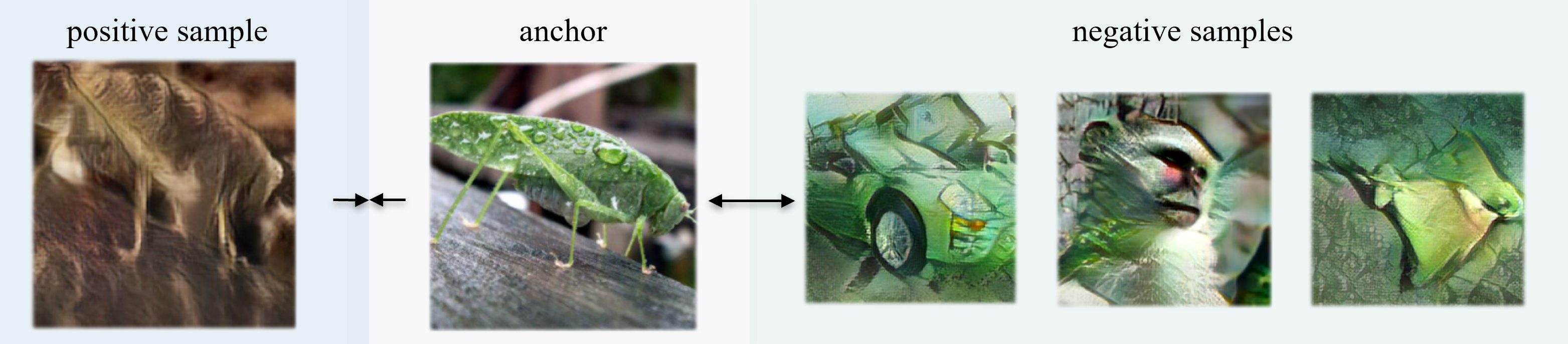
Figure 9: Example for sampling contrastive pairs for reducing texture bias

Datasets: We evaluate models’ shape bias on two datasets: Stylized ImageNet-$9$ and ImageNet-$9$-Sketch. We generate the Stylized ImageNet-$9$ using the same algorithm (AdaIN [Huang and Belongie(2017)]) as the original Stylized ImageNet [Geirhos et al.(2019)Geirhos, Rubisch, Michaelis, Bethge, Wichmann, and Brendel]. ImageNet-$9$-Sketch is created by mapping the classes in ImageNet-Sketch [Wang et al.(2019a)Wang, Ge, Lipton, and Xing] to classes in ImageNet-$9$. Models with high shape bias are expected to have better accuracy on these datasets, as the texture information in these datasets is either randomized or removed and hence provides no useful information on the class label.

The performance of S-CLAD+ and S-CLAD is compared against two baselines, Base(IN9) and Base(SIN9), where the latter is a baseline model trained on stylized images from ImageNet-$9$ in a fully supervised setting. The results are presented in Table 7. We can see that, both S-CLAD and S-CLAD+ outperform the Base(IN9) baseline with a large margin on Stylized ImageNet-$9$ and ImageNet-$9$-Sketch, indicating their texture bias is mitigated. Moreover, we again observe that there is almost no accuracy trade-off on the Original ImageNet-9 for S-CLAD and S-CLAD+, whereas Base(SIN9) suffers from performance drop on the Original ImageNet-9. Note that, no sketch images are included in S-CLAD+ and S-CLAD’s training process, and they still have a performance gain of around 20% on the ImageNet-$9$-Sketch dataset. This performance gain is because the model is focusing more on shape information.

Model	Original ImageNet-$9$	Stylized ImageNet-$9$	ImageNet-$9$-Sketch
Base (IN9)	96.0	53.6	40.1
Base (SIN9)	91.5	75.1	58.0
S-CLAD	95.1	74.4	61.0
S-CLAD+	95.5	76.7	58.6

Table 7: Accuracy comparison for S-CLAD+ and S-CLAD, against Base(IN9) on three datasets. The accuracy on Stylized and Sketch dataset indicates model’s shape bias.

V Cross-Evaluation

In this section, we cross-evalutate whether background-debiased models (CLAD and CLAD+) generalize better to the texture variation, and vise-versa. Firstly, we evaluate the shape bias of CLAD and CLAD+, compared against Base(IN9) on Stylized ImageNet-$9$ and ImageNet-$9$-Sketch.

Model	Original ImageNet-$9$	Stylized ImageNet-$9$	ImageNet-$9$-Sketch
Base (IN9)	96.0	53.6	40.1
CLAD	95.9	54.3	39.7
CLAD+	95.6	53.7	41.2

Table 8: Evaluation of shape bias for CLAD, CLAD+, compared against Base(IN9).

The results show a minor improvement by CLAD and CLAD+ on Stylized ImageNet-$9$ and ImageNet-$9$-Sketch respectively. This can explained due to the fact that by removing background bias, we focus more on both the foreground shape and texture information. Hence, our model may still use the texture information from the foreground for classification along with its shape. Thus, its performance on datasets which transform the texture of the foreground and background together is not improved drastically. This also implies that background debiasing alone is not sufficient for texture debiasing.

Model	Original$\uparrow$	Only-FG$\uparrow$	Mixed-Rand$\uparrow$	Mixed-Same$\uparrow$	Only-BG-T$\downarrow$	BG-Gap$\downarrow$
Base (IN9)	96.0	86.0	73.4	87.5	42.9	14.1
S-CLAD	95.0	87.5	78.9	89.3	40.9	10.4
S-CLAD+	95.5	87.4	78.1	88.5	38.1	10.4

Table 9: Evaluation of S-CLAD, S-CLAD+ on Background Challenge, compared against Base(IN9).

We then test S-CLAD and S-CLAD+ on the Background Challenge datasets [Xiao et al.(2020)Xiao, Engstrom, Ilyas, and Madry]. As shown in Table. 9, we find that inducing shape bias helps mitigate background bias to some extent. This can be explained by the increased focus on shape of the object which is usually in the foreground, while also ignoring the background information. However, texture-debiased model, S-CLAD and S-CLAD+ alone are not sufficient to reproduce our state of the art results we had from CLAD and CLAD+ on Background Challenge.

References

- [Baker et al.(2018)Baker, Lu, Erlikhman, and Kellman] Nicholas Baker, Hongjing Lu, Gennady Erlikhman, and Philip J Kellman. Deep convolutional networks do not classify based on global object shape. PLoS computational biology, 2018.
- [Barbu et al.(2019)Barbu, Mayo, Alverio, Luo, Wang, Gutfreund, Tenenbaum, and Katz] Andrei Barbu, David Mayo, Julian Alverio, William Luo, Christopher Wang, Dan Gutfreund, Josh Tenenbaum, and Boris Katz. Objectnet: A large-scale bias-controlled dataset for pushing the limits of object recognition models. Advances in neural information processing systems, 2019.
- [Beery et al.(2018)Beery, Van Horn, and Perona] Sara Beery, Grant Van Horn, and Pietro Perona. Recognition in terra incognita. European conference on computer vision, 2018.
- [Benz et al.(2021)Benz, Ham, Zhang, Karjauv, and Kweon] Philipp Benz, Soomin Ham, Chaoning Zhang, Adil Karjauv, and In So Kweon. Adversarial robustness comparison of vision transformer and mlp-mixer to cnns. arXiv preprint arXiv:2110.02797, 2021.
- [Brendel and Bethge(2019)] Wieland Brendel and Matthias Bethge. Approximating CNNs with bag-of-local-features models works surprisingly well on imagenet. International Conference on Learning Representations, 2019.
- [Chen et al.(2020)Chen, Kornblith, Norouzi, and Hinton] Ting Chen, Simon Kornblith, Mohammad Norouzi, and Geoffrey Hinton. A simple framework for contrastive learning of visual representations. International conference on machine learning, 2020.
- [Geirhos et al.(2017)Geirhos, Janssen, Schütt, Rauber, Bethge, and Wichmann] Robert Geirhos, David HJ Janssen, Heiko H Schütt, Jonas Rauber, Matthias Bethge, and Felix A Wichmann. Comparing deep neural networks against humans: object recognition when the signal gets weaker. arXiv preprint arXiv:1706.06969, 2017.
- [Geirhos et al.(2019)Geirhos, Rubisch, Michaelis, Bethge, Wichmann, and Brendel] Robert Geirhos, Patricia Rubisch, Claudio Michaelis, Matthias Bethge, Felix A Wichmann, and Wieland Brendel. Imagenet-trained cnns are biased towards texture; increasing shape bias improves accuracy and robustness. International Conference on Learning Representations, 2019.
- [Grill et al.(2020)Grill, Strub, Altché, Tallec, Richemond, Buchatskaya, Doersch, Avila Pires, Guo, Gheshlaghi Azar, et al.] Jean-Bastien Grill, Florian Strub, Florent Altché, Corentin Tallec, Pierre Richemond, Elena Buchatskaya, Carl Doersch, Bernardo Avila Pires, Zhaohan Guo, Mohammad Gheshlaghi Azar, et al. Bootstrap your own latent-a new approach to self-supervised learning. Advances in neural information processing systems, 2020.
- [Gutmann and Hyvärinen(2010)] Michael Gutmann and Aapo Hyvärinen. Noise-contrastive estimation: A new estimation principle for unnormalized statistical models. International conference on artificial intelligence and statistics, 2010.
- [Hadsell et al.(2006)Hadsell, Chopra, and LeCun] Raia Hadsell, Sumit Chopra, and Yann LeCun. Dimensionality reduction by learning an invariant mapping. IEEE conference on computer vision and pattern recognition, 2006.
- [He et al.(2016)He, Zhang, Ren, and Sun] Kaiming He, Xiangyu Zhang, Shaoqing Ren, and Jian Sun. Deep residual learning for image recognition. 2016.
- [He et al.(2020)He, Fan, Wu, Xie, and Girshick] Kaiming He, Haoqi Fan, Yuxin Wu, Saining Xie, and Ross Girshick. Momentum contrast for unsupervised visual representation learning. IEEE conference on computer vision and pattern recognition, 2020.
- [Hermann et al.(2020)Hermann, Chen, and Kornblith] Katherine Hermann, Ting Chen, and Simon Kornblith. The origins and prevalence of texture bias in convolutional neural networks. Advances in Neural Information Processing Systems, 2020.
- [Huang and Belongie(2017)] Xun Huang and Serge Belongie. Arbitrary style transfer in real-time with adaptive instance normalization. IEEE international conference on computer vision, 2017.
- [Islam et al.(2021)Islam, Kowal, Esser, Jia, Ommer, Derpanis, and Bruce] Md Amirul Islam, Matthew Kowal, Patrick Esser, Sen Jia, Björn Ommer, Konstantinos G. Derpanis, and Neil Bruce. Shape or texture: Understanding discriminative features in {cnn}s. International Conference on Learning Representations, 2021.
- [Kakogeorgiou et al.(2022)Kakogeorgiou, Gidaris, Psomas, Avrithis, Bursuc, Karantzalos, and Komodakis] Ioannis Kakogeorgiou, Spyros Gidaris, Bill Psomas, Yannis Avrithis, Andrei Bursuc, Konstantinos Karantzalos, and Nikos Komodakis. What to hide from your students: Attention-guided masked image modeling. arXiv preprint arXiv:2203.12719, 2022.
- [Khani and Liang(2021)] Fereshte Khani and Percy Liang. Removing spurious features can hurt accuracy and affect groups disproportionately. ACM Conference on Fairness, Accountability, and Transparency, 2021.
- [Khosla et al.(2020)Khosla, Teterwak, Wang, Sarna, Tian, Isola, Maschinot, Liu, and Krishnan] Prannay Khosla, Piotr Teterwak, Chen Wang, Aaron Sarna, Yonglong Tian, Phillip Isola, Aaron Maschinot, Ce Liu, and Dilip Krishnan. Supervised contrastive learning. Advances in Neural Information Processing Systems, 2020.
- [Kingma and Ba(2015)] Diederik P Kingma and Jimmy Ba. Adam: A method for stochastic optimization. International Conference on Learning Representations, 2015.
- [Lee et al.(2022)Lee, Hwang, Kang, and Zhang] Sangjun Lee, Inwoo Hwang, Gi-Cheon Kang, and Byoung-Tak Zhang. Improving robustness to texture bias via shape-focused augmentation. IEEE Conference on Computer Vision and Pattern Recognition, 2022.
- [Liu et al.(2021)Liu, Yan, and Alahi] Yuejiang Liu, Qi Yan, and Alexandre Alahi. Social nce: Contrastive learning of socially-aware motion representations. IEEE International Conference on Computer Vision, 2021.
- [Lo et al.(2021)Lo, Chang, Chiu, Huang, Chen, Chang, and Jou] Yi-Chen Lo, Chia-Che Chang, Hsuan-Chao Chiu, Yu-Hao Huang, Chia-Ping Chen, Yu-Lin Chang, and Kevin Jou. Clcc: Contrastive learning for color constancy. IEEE Conference on Computer Vision and Pattern Recognition, 2021.
- [Machiraju et al.(2022)Machiraju, Choung, Herzog, and Frossard] Harshitha Machiraju, Oh-Hyeon Choung, Michael H Herzog, and Pascal Frossard. Empirical advocacy of bio-inspired models for robust image recognition. arXiv preprint arXiv:2205.09037, 2022.
- [Miller(1995)] George A Miller. Wordnet: a lexical database for english. Communications of the ACM, 1995.
- [Mo et al.(2021)Mo, Kang, Sohn, Li, and Shin] Sangwoo Mo, Hyunwoo Kang, Kihyuk Sohn, Chun-Liang Li, and Jinwoo Shin. Object-aware contrastive learning for debiased scene representation. Advances in Neural Information Processing Systems, 2021.
- [Moayeri et al.(2022)Moayeri, Pope, Balaji, and Feizi] Mazda Moayeri, Phillip Pope, Yogesh Balaji, and Soheil Feizi. A comprehensive study of image classification model sensitivity to foregrounds, backgrounds, and visual attributes. IEEE Conference on Computer Vision and Pattern Recognition, 2022.
- [Oord et al.(2018)Oord, Li, and Vinyals] Aaron van den Oord, Yazhe Li, and Oriol Vinyals. Representation learning with contrastive predictive coding. arXiv preprint arXiv:1807.03748, 2018.
- [Ortiz-Jimenez et al.(2020)Ortiz-Jimenez, Modas, Moosavi, and Frossard] Guillermo Ortiz-Jimenez, Apostolos Modas, Seyed-Mohsen Moosavi, and Pascal Frossard. Hold me tight! influence of discriminative features on deep network boundaries. Advances in Neural Information Processing Systems, 2020.
- [Qin et al.(2020)Qin, Zhang, Huang, Dehghan, Zaiane, and Jagersand] Xuebin Qin, Zichen Zhang, Chenyang Huang, Masood Dehghan, Osmar R Zaiane, and Martin Jagersand. U2-net: Going deeper with nested u-structure for salient object detection. Pattern recognition, 2020.
- [Rother et al.(2004)Rother, Kolmogorov, and Blake] Carsten Rother, Vladimir Kolmogorov, and Andrew Blake. "grabcut" interactive foreground extraction using iterated graph cuts. ACM transactions on graphics (TOG), 2004.
- [Ryali et al.(2021)Ryali, Schwab, and Morcos] Chaitanya K Ryali, David J Schwab, and Ari S Morcos. Leveraging background augmentations to encourage semantic focus in self-supervised contrastive learning. arXiv preprint arXiv:2103.12719, 2021.
- [Sameni et al.(2022)Sameni, Jenni, and Favaro] Sepehr Sameni, Simon Jenni, and Paolo Favaro. Dilemma: Self-supervised shape and texture learning with transformers. arXiv preprint arXiv:2204.04788, 2022.
- [Sehwag et al.(2020)Sehwag, Oak, Chiang, and Mittal] Vikash Sehwag, Rajvardhan Oak, Mung Chiang, and Prateek Mittal. Time for a background check! uncovering the impact of background features on deep neural networks. arXiv preprint arXiv:2006.14077, 2020.
- [Smilkov et al.(2017)Smilkov, Thorat, Kim, Viégas, and Wattenberg] Daniel Smilkov, Nikhil Thorat, Been Kim, Fernanda Viégas, and Martin Wattenberg. Smoothgrad: removing noise by adding noise. arXiv preprint arXiv:1706.03825, 2017.
- [Szegedy et al.(2015)Szegedy, Liu, Jia, Sermanet, Reed, Anguelov, Erhan, Vanhoucke, and Rabinovich] Christian Szegedy, Wei Liu, Yangqing Jia, Pierre Sermanet, Scott Reed, Dragomir Anguelov, Dumitru Erhan, Vincent Vanhoucke, and Andrew Rabinovich. Going deeper with convolutions. IEEE conference on computer vision and pattern recognition, 2015.
- [Taghanaki et al.(2021)Taghanaki, Choi, Khasahmadi, and Goyal] Saeid A Taghanaki, Kristy Choi, Amir Hosein Khasahmadi, and Anirudh Goyal. Robust representation learning via perceptual similarity metrics. International Conference on Machine Learning, 2021.
- [Voulodimos et al.(2018)Voulodimos, Doulamis, Doulamis, and Protopapadakis] Athanasios Voulodimos, Nikolaos Doulamis, Anastasios Doulamis, and Eftychios Protopapadakis. Deep learning for computer vision: A brief review. Computational intelligence and neuroscience, 2018.
- [Wang et al.(2019a)Wang, Ge, Lipton, and Xing] Haohan Wang, Songwei Ge, Zachary Lipton, and Eric P Xing. Learning robust global representations by penalizing local predictive power. Advances in Neural Information Processing Systems, 2019a.
- [Wang et al.(2019b)Wang, Zhao, Yatskar, Chang, and Ordonez] Tianlu Wang, Jieyu Zhao, Mark Yatskar, Kai-Wei Chang, and Vicente Ordonez. Balanced datasets are not enough: Estimating and mitigating gender bias in deep image representations. IEEE International Conference on Computer Vision, 2019b.
- [Wei et al.(2022)Wei, Hu, Xie, Zhang, Cao, Bao, Chen, and Guo] Yixuan Wei, Han Hu, Zhenda Xie, Zheng Zhang, Yue Cao, Jianmin Bao, Dong Chen, and Baining Guo. Contrastive learning rivals masked image modeling in fine-tuning via feature distillation. arXiv preprint arXiv:2205.14141, 2022.
- [Xiao et al.(2020)Xiao, Engstrom, Ilyas, and Madry] Kai Yuanqing Xiao, Logan Engstrom, Andrew Ilyas, and Aleksander Madry. Noise or signal: The role of image backgrounds in object recognition. International Conference on Learning Representations, 2020.
- [Yin et al.(2019)Yin, Gontijo Lopes, Shlens, Cubuk, and Gilmer] Dong Yin, Raphael Gontijo Lopes, Jon Shlens, Ekin Dogus Cubuk, and Justin Gilmer. A fourier perspective on model robustness in computer vision. Advances in Neural Information Processing Systems, 2019.
- [Zhang et al.(2022)Zhang, Li, Liu, Zhang, Su, Zhu, Ni, and Shum] Hao Zhang, Feng Li, Shilong Liu, Lei Zhang, Hang Su, Jun Zhu, Lionel M Ni, and Heung-Yeung Shum. Dino: Detr with improved denoising anchor boxes for end-to-end object detection. arXiv preprint arXiv:2203.03605, 2022.
- [Zhao and Gordon(2019)] Han Zhao and Geoff Gordon. Inherent tradeoffs in learning fair representations. Advances in neural information processing systems, 2019.
- [Zhu et al.(2017)Zhu, Xie, and Yuille] Zhuotun Zhu, Lingxi Xie, and Alan Yuille. Object recognition with and without objects. International Joint Conference on Artificial Intelligence, 2017.