Geometric discretization of diffeomorphisms

Abstract.

Many partial differential equations in mathematical physics describe the evolution of a time-dependent vector field. Examples arise in compressible fluid dynamics, shape analysis, optimal transport, and shallow water equations. The flow of such a vector field generates a diffeomorphism, which can be viewed as the Lagrangian variable corresponding to the Eulerian vector field. From both computational and theoretical perspectives, it is natural to seek finite-dimensional analogs of vector fields and diffeomorphisms, constructed in such a way that the underlying geometric and algebraic properties persist (in particular, the induced Lie–Poisson structure). Here, we develop such a geometric discretization of the group of diffeomorphisms on a two-dimensional Kähler manifold, with special emphasis on the sphere. Our approach builds on quantization theory, combined with complexification of Zeitlin’s model for incompressible two-dimensional hydrodynamics. Thus, we extend Zeitlin’s approach from the incompressible to the compressible case. We provide a numerical example and discuss potential applications of the new, geometric discretization.

1. Introduction

Euler’s equations describe the evolution of a homogeneous, incompressible fluid. On a Riemannian manifold $M$, they are given by

(1) $$\begin{gathered}\dot{v}+v\cdot\nabla v=-\nabla p,\\ \operatorname{div}v=0,\end{gathered}$$

where $v$ is a divergence-free vector field for the fluid velocity, $p$ is a pressure potential, and $\nabla v$ is the co-variant derivative.

Arnold (1966) showed that Equation 1 has a remarkable geometric structure: it is a geodesic equation on the group of volume-preserving diffeomorphisms equipped with a right-invariant $\mathrm{L}^{2}$ metric. Many non-linear equations arise this way. Indeed, by varying the group and the metric, a large class of equations from different areas of physics and mathematics are obtained, for instance, the rigid body equations, the KdV equation, and other shallow water equations, or equations in shape analysis (see, for example, the monograph by Arnold and Khesin (1998) for an overview).

When $M$ is two-dimensional, Equation 1 can be rewritten as the vorticity equation,

(2) $$\dot{\omega}=\{-\psi,\omega\},\qquad\psi=-\Delta^{-1}\omega.$$

Here, $\omega$ and $\psi$ are smooth functions called vorticity function and stream function, and $\{\cdot,\cdot\}$ denotes the Poisson bracket. The velocity is recovered as $v=\nabla^{\perp}\psi$ where $\nabla^{\perp}$ is the skew-gradient. System (2) is an example of a Lie–Poisson system. See Marsden and Ratiu (1999) and the references therein for more details on systems of this type. Hereon, we focus on the case when $M$ is the sphere $\amsmathbb{S}^{2}$, although much of the theory, albeit not necessarily the numerics, can be extended to compact, quantizable Kähler manifolds.

A spatial discretization of Equation 2 was introduced by Zeitlin (1991, 2004). This discretization, often called Zeitlin’s model, builds on quantization theory, see Hoppe (1989); Bordemann et al. (1991, 1994); Le Floch (2018).

Zeitlin’s model retains the underlying Lie–Poisson structure of Equation 2, resulting in a finite-dimensional isospectral flow on matrices,

(3) $$\dot{W}=[-P,W],\qquad P=-\Delta_{N}^{-1}W.$$

Here, $W$ is the skew-Hermitian vorticity matrix and $P$ is the skew-Hermitian stream matrix. The operator $\Delta_{N}$ is the Hoppe–Yau Laplacian (Hoppe and Yau, 1998). For more details on Equation 3 and the quantization scheme, see Zeitlin (1991, 2004) and Modin and Viviani (2020). Gallagher (2002) established convergence of solutions of Zeitlin’s model to solutions of the vorticity equation (for the torus case originally considered by Zeitlin).

Zeitlin’s model can be used to discretize fluid-type equations on $\amsmathbb{S}^{2}$ described by divergence-free vector fields. A natural question is if this approach can be extended to equations involving general (smooth) vector fields. As an example, consider the EPDiff equation on $\amsmathbb{S}^{2}$, which originates from the geodesic equation on $\operatorname{Diff}(\amsmathbb{S}^{2})$ equipped with a right-invariant $\mathrm{H}^{k}$-metric. It is given by

(4) $$\dot{m}=\nabla_{v}^{T}m-\nabla_{m}v+\operatorname{div}(v)m,$$

$$m=(1-\alpha\Delta)^{k}v.$$

Here $v$ is a vector field, $\nabla$ is the covariant derivative, $\nabla^{T}$ is its transpose with respect to $\mathrm{L}^{2}$ and $\alpha$ is a positive constant. These equations were derived by Mumford (1998) in the context of shape analysis (cf. Younes (2010)).

The vector field $v$ in Equation 4 is analogous to the vector field $v$ in Euler’s equations (1). An important difference, however, is that for EPDiff the vector field $v$ is not divergence-free. The goal of this paper is to extend the quantization-based discretization method of Zeitlin from divergence-free vector fields, such as in Equation 1, to generic vector fields, such as in Equation 4.

The paper is structured as follows. In Section 2 we briefly outline the theory of the class of systems considered in this paper and derive the vorticity formulation of Equation 4. In Section 3 we describe the quantization-based discretization scheme and provide its extension to the manifold of all diffeomorphisms on the sphere. A computational example is performed in Section 4. Finally, in Section 5, we discuss future directions, specifically settings for which the method presented in this paper could prove useful.

Acknowledgements. This work was supported by the Wallenberg AI, Autonomous Systems and Software Program (WASP) funded by the Knut and Alice Wallenberg Foundation. This work was also supported by the Swedish Research Council, grant number 2022-03453, and the Knut and Alice Wallenberg Foundation, grant number WAF2019.0201. The authors would like to thank Paolo Cifani, Erwin Luesink, and Milo Viviani for fruitful discussions related to this work.

2. Background: Kähler geometry and Poisson brackets

In this section, we describe the theoretical foundations of the quantization method. We begin with the geometric setting. The sphere $\amsmathbb{S}^{2}$ is a Kähler manifold: its area-form is a symplectic form $\Omega$ compatible with the standard round Riemannian metric $g$ via an integrable almost complex structure $J:T\amsmathbb{S}^{2}\to T\amsmathbb{S}^{2}$, i.e., a smooth field of automorphisms of the tangent bundle such that $J^{2}=-\mathrm{id}$ and $g(\cdot,\cdot)=-\Omega(J\cdot,\cdot)$. For details on Kähler manifolds, with a notation similar to ours, see the monograph by da Silva (2008).

The gradient $\nabla f$ of a smooth function $f\in C^{\infty}(\amsmathbb{S}^{2},\amsmathbb{R})$ is defined by

$$\,\mathrm{d}f(\cdot)=g(\nabla f,\cdot),$$

where $\,\mathrm{d}$ is the exterior derivative. The Hamiltonian vector field $X_{f}$ of $f$ is similarly defined by the relation

$$\,\mathrm{d}f(\cdot)=\Omega(X_{f},\cdot).$$

Since

$$\,\mathrm{d}f(\cdot)=g(\nabla f,\cdot)=-\Omega(J\nabla f,\cdot),$$

we have that $-J\nabla f=X_{f}$. This means that Hamiltonian vector fields are obtained by point-wise $\pi/2$ rotation of corresponding gradient vector fields.

Quantization unfolds from the Poisson algebra of smooth functions $(C^{\infty}(\amsmathbb{S}^{2},\amsmathbb{R}),\{\cdot,\cdot\})$, where $\{\cdot,\cdot\}\colon C^{\infty}(\amsmathbb{S}^{2},\amsmathbb{R})\times C^{\infty}(\amsmathbb{S}^{2},\amsmathbb{R})\to C^{\infty}(\amsmathbb{S}^{2},\amsmathbb{R})$ is the Poisson bracket, defined by

(5) $$\{f,g\}=\Omega(X_{f},X_{g})=X_{g}(f).$$

Explicitly, in the standard, unit radius embedding $\amsmathbb{S}^{2}\subset\amsmathbb{R}^{3}$, it is given by

$$\{f,g\}(\mathbf{r})=(\mathbf{r}\times\nabla g(\mathbf{r}))\cdot\nabla f(\mathbf{r}).$$

The Poisson bracket is skew-symmetric and satisfies Leibniz’s rule and the Jacobi identity. In particular, it is a Lie bracket. Further,

(6) $$[X_{f},X_{g}]=-X_{\{f,g\}},$$

where $[\cdot,\cdot]$ is the Lie bracket of vector fields. Equation 6 means that $f\mapsto X_{f}$ is an anti-Poisson morphism between $(C^{\infty}(\amsmathbb{S}^{2},\amsmathbb{R}),\{\cdot,\cdot\})$ and $(\mathfrak{X}_{\Omega}(\amsmathbb{S}^{2}),[\cdot,\cdot])$, where $\mathfrak{X}_{\Omega}(\amsmathbb{S}^{2})$ denotes Hamiltonian vector fields on $\amsmathbb{S}^{2}$. The space of all vector fields is denoted $\mathfrak{X}(\amsmathbb{S}^{2})$. Notice that $\mathfrak{X}_{\Omega}(\amsmathbb{S}^{2})$ is a sub-algebra of $\mathfrak{X}(\amsmathbb{S}^{2})$.

The original approach of Zeitlin is applicable to $\mathfrak{X}_{\Omega}(\amsmathbb{S}^{2})$ via the identification $f\leftrightarrow X_{f}$ and the property in Equation 6. For the intended extension, we thus need an anti-Poisson morphism between the space $\mathfrak{X}(\amsmathbb{S}^{2})$ of vector fields and some extended Poisson algebra of functions. To see which space of functions this is, we use a standard result in Kähler geometry (cf. Le Floch (2018)): the Hodge decomposition theorem states, since $\amsmathbb{S}^{2}$ has trivial first cohomology, that any $v\in\mathfrak{X}(\amsmathbb{S}^{2})$ can be decomposed as

$$v=X_{h}+\nabla f,$$

for $f,h\in C^{\infty}(\amsmathbb{S}^{2},\amsmathbb{R})$. Note that $Jv=\nabla h-X_{f}$. Thus, $-f$ generates the Hamiltonian component of the rotated field $Jv$, while $h$ generates the gradient component. We capture precisely this behavior by letting imaginary functions generate gradient vector fields, while real functions generate Hamiltonian vector fields. Indeed, multiplying the vector field with $J$ corresponds to multiplying the generator with the imaginary unit $i$. In other words, the real vector field $v$ is given as the “Hamiltonian” vector field of a complex function. To make this precise, the Hamiltonian vector field of a purely imaginary function $if\in iC^{\infty}(\amsmathbb{S}^{2},\amsmathbb{R})$ is given by

$$X_{if}\coloneqq JX_{f}=-J^{2}\nabla f=\nabla f.$$

Thus, given a complex-valued function $\psi\in C^{\infty}(\amsmathbb{S}^{2},\amsmathbb{C})$,

(7) $$X_{\psi}=X_{\operatorname{Re}\psi+i\operatorname{Im}\psi}=X_{\operatorname{Re}\psi}+\nabla\operatorname{Im}\psi.$$

Therefore,

$$JX_{\psi}=\nabla\operatorname{Re}\psi-X_{\operatorname{Im}\psi}=X_{-\operatorname{Im}\psi+i\operatorname{Re}\psi}=X_{i\psi}.$$

Next, the Poisson algebra structure on $C^{\infty}(\amsmathbb{S}^{2},\amsmathbb{C})$ is readily obtained by complexifying $(C^{\infty}(\amsmathbb{S}^{2},\amsmathbb{R}),\{\})$. Explicitly, the bracket on $C^{\infty}(\amsmathbb{S}^{2},\amsmathbb{C})$ is given by

$$\{{\psi_{1}},{\psi_{2}}\}{C}=\{\operatorname{Re}{\psi_{1}},\operatorname{Re}{\psi_{2}}\}-\{\operatorname{Im}{\psi_{1}},\operatorname{Im}{\psi_{2}}\}$$

$$\qquad+i\left(\{\operatorname{Im}{\psi_{1}},\operatorname{Re}{\psi_{2}}\}+\{\operatorname{Re}{\psi_{1}},\operatorname{Im}{\psi_{2}}\}\right),$$

where $\{\cdot,\cdot\}:C^{\infty}(\amsmathbb{S}^{2},\amsmathbb{R})\times C^{\infty}(\amsmathbb{S}^{2},\amsmathbb{R})\to C^{\infty}(\amsmathbb{S}^{2},\amsmathbb{R})$ is the standard Poisson bracket on $C^{\infty}(\amsmathbb{S}^{2},\amsmathbb{R})$. By properties inherited from the real-valued case, $(C^{\infty}(\amsmathbb{S}^{2},\amsmathbb{C}),\{\cdot,\cdot\}{C})$ is a Poisson algebra.

The infinitesimal action of a Hamiltonian vector field on an imaginary function is determined by the Poisson bracket. Indeed, as $JX_{g}=X_{ig}$, we have that

$$JX_{g}(f)=X_{ig}(f)\coloneqq i\{f,g\},$$

where $f,g\in C^{\infty}(\amsmathbb{S}^{2},\amsmathbb{R})$. While $JX_{g}$ is a real vector field, applying it to a real-valued function results in an imaginary function. Thus, we have for ${\psi_{1}},{\psi_{2}}\in C^{\infty}(\amsmathbb{S}^{2},\amsmathbb{C})$,

(8) $$\begin{split}&X_{\psi_{2}}({\psi_{1}})=X_{\operatorname{Re}{\psi_{2}}}({\psi_{1}})+JX_{\operatorname{Im}{\psi_{2}}}({\psi_{1}})\\ &=X_{\operatorname{Re}{\psi_{2}}}(\operatorname{Re}{\psi_{1}})+iX_{\operatorname{Re}{\psi_{2}}}(\operatorname{Im}{\psi_{1}})+X_{i\operatorname{Im}{\psi_{2}}}(\operatorname{Re}{\psi_{1}})+iX_{i\operatorname{Im}{\psi_{2}}}(\operatorname{Im}{\psi_{1}})\\ &=\{\operatorname{Re}{\psi_{1}},\operatorname{Re}{\psi_{2}}\}-\{\operatorname{Im}{\psi_{1}},\operatorname{Im}{\psi_{2}}\}\\ &\qquad+i\left(\{\operatorname{Re}{\psi_{1}},\operatorname{Im}{\psi_{2}}\}+\{\operatorname{Im}{\psi_{1}},\operatorname{Re}{\psi_{2}}\}\right)=\{{\psi_{1}},{\psi_{2}}\}_{\amsmathbb{C}}.\end{split}$$

Using Equation 8, we can relate the Lie bracket of real vector fields with the complex Poisson bracket by the following well-known lemma.

Lemma 2.1.

Let ${\psi_{1}},{\psi_{2}}\in C^{\infty}(\amsmathbb{S}^{2},\amsmathbb{C})$. Equation 7 determines an anti-Poisson morphism between $(C^{\infty}(\amsmathbb{S}^{2},\amsmathbb{C}),\{\cdot,\cdot\}{C})$ and $(\mathfrak{X}(M),[\cdot,\cdot])$, i.e,

(9) $$-X_{\{{\psi_{1}},{\psi_{2}}\}{C}}=[X_{\psi_{1}},X_{\psi_{2}}].$$

Proof.

$X_{\psi_{1}}$ and $X_{\psi_{2}}$ are both real vector fields, so the action of $[X_{\psi_{1}},X_{\psi_{2}}]$ on a smooth complex function $\omega$ is also a smooth complex function. By the definition of the real Lie bracket of vector fields,

$$[X_{\psi_{1}},X_{\psi_{2}}](\omega)=X_{\psi_{1}}(X_{\psi_{2}}(\omega))-X_{\psi_{2}}(X_{\psi_{1}}(\omega)).$$

By applying Equation 8 twice to each term, we obtain

$$[X_{\psi_{1}},X_{\psi_{2}}](\omega)=\{{\psi_{1}},\{{\psi_{2}},\omega\}\}{C}+\{{\psi_{2}},\{\omega,{\psi_{1}}\}\}{C}=-\{\omega,\{{\psi_{1}},{\psi_{2}}\}\}{C}=-X_{\{{\psi_{1}},{\psi_{2}}\}}(\omega),$$

where the first equality is due to the Jacobi identity and the second follows from Equation 8. ∎

Equation 9 is not an isomorphism. Indeed, all constant functions are mapped to the zero vector field. Since constant functions form the center of the Poisson algebra $(C^{\infty}(\amsmathbb{S}^{2},\amsmathbb{C}),\{\cdot,\cdot\}{C})$, we obtain the reduced Poisson algebra $(C^{\infty}(\amsmathbb{S}^{2},\amsmathbb{C})/\amsmathbb{C},\{\cdot,\cdot\}{C})$, anti-Poisson isomorphic to $\mathfrak{X}(\amsmathbb{S}^{2})$.

As previously noted, Equation 4 is the geodesic equation on the infinite-dimensional Lie group $\operatorname{Diff}(\amsmathbb{S}^{2})$ equipped with a right-invariant $\mathrm{H}^{k}$-metric. Moreover, Equation 4 is an example of an Euler–Arnold equation. From the Hamiltonian perspective, on a general Lie algebra $\mathfrak{g}$, these equations are

(10) $$\dot{\mu}=\operatorname{ad}_{\delta_{\mu}H}^{*}\mu.$$

Here, $\mu\in\mathfrak{g}^{*}$, $H\in C^{\infty}(\mathfrak{g}^{*},\amsmathbb{R})$ is the Hamiltonian function and $\delta_{\mu}H$ denotes its variational derivative with respect to $\mu$. The mapping $\operatorname{ad}^{*}:\mathfrak{g}\to\operatorname{End}(\mathfrak{g}^{*})$ is the dual, under the canonical dual pairing, of the adjoint representation $\operatorname{ad}:\mathfrak{g}\to\operatorname{End}(\mathfrak{g})$. This way, Equation 4 is retrieved with $\mathfrak{g}=\mathfrak{X}(\amsmathbb{S}^{2})$ and the Hamiltonian

(11) $$H(m)=\int_{\amsmathbb{S}^{2}}m\cdot(1-\alpha\Delta)^{-k}m\Omega=\int_{\amsmathbb{S}^{2}}(1-\alpha\Delta)^{k}v\cdot v\Omega,$$

where $m=(1-\alpha\Delta)^{k}v\in\mathfrak{X}(M)^{*}$.

As mentioned, the mapping $\psi\mapsto X_{\psi}$ provides an isomorphism between the two Lie algebras $(C^{\infty}(\amsmathbb{S}^{2},\amsmathbb{C})/\amsmathbb{C},\{\cdot,\cdot\}{C})$ and $\mathfrak{X}(\amsmathbb{S}^{2})$, so a first step towards a complexified vorticity formulation of Equation 4 is to derive the corresponding Euler–Arnold equation on $(C^{\infty}(\amsmathbb{S}^{2},\amsmathbb{C})/\amsmathbb{C},\{\cdot,\cdot\}{C})$.

As the Euler–Arnold equation evolves on the dual of the algebra, we note that the (smooth) dual of $(C^{\infty}(\amsmathbb{S}^{2},\amsmathbb{C})/\amsmathbb{C},\{\cdot,\cdot\}{C})$ is the annihilator of constant functions in the space of top-forms. A top-form $\beta=\omega\Omega$, where $\omega\in C^{\infty}(\amsmathbb{S}^{2},\amsmathbb{C})$, acts on a function $\psi\in C^{\infty}(\amsmathbb{S}^{2},\amsmathbb{C})$ by

(12) $$\langle\beta,\psi\rangle=\int_{\amsmathbb{S}^{2}}\omega\bar{\psi}\Omega.$$

Since top-forms can be identified with smooth functions, the (smooth) dual of $C^{\infty}(\amsmathbb{S}^{2},\amsmathbb{C})/\amsmathbb{C}$ is isomorphic to $C^{\infty}_{0}(\amsmathbb{S}^{2},\amsmathbb{C})$, the smooth complex-valued functions with vanishing mean.

The next step is to compute $\operatorname{ad}_{\psi}^{*}\colon C^{\infty}_{0}(\amsmathbb{S}^{2},\amsmathbb{C})\to C^{\infty}_{0}(\amsmathbb{S}^{2},\amsmathbb{C})$. By definition,

$$\langle\operatorname{ad}_{\psi}^{*}\omega,\xi\rangle=\langle\omega,\operatorname{ad}_{\psi}\xi\rangle=\int_{\amsmathbb{S}^{2}}\omega\overline{\{\psi,\xi\}_{\amsmathbb{C}}}\Omega=\int_{\amsmathbb{S}^{2}}\omega\{\bar{\psi},\bar{\xi}\}_{\amsmathbb{C}}\Omega=$$

$$\int_{\amsmathbb{S}^{2}}\left(\{\bar{\psi},\omega\bar{\xi}\}_{\amsmathbb{C}}-\bar{\xi}\{\bar{\psi},\omega\}_{\amsmathbb{C}}\right)\Omega=\langle\{-\bar{\psi},\omega\}{C},\xi\rangle,$$

where, in the fourth equality, Leibniz’s rule is used. Therefore, $\operatorname{ad}_{\psi}^{*}\omega=\{-\bar{\psi},\omega\}{C}$.

The final step is to find the canonical relationship between $\omega$ and $\psi$ determined by the Hamiltonian of the EPDiff equation, i.e., Equation 11.

The Hamiltonian $\tilde{H}:C^{\infty}_{0}(\amsmathbb{S}^{2},\amsmathbb{C})\to\amsmathbb{R}$ is given by

(13) $$\tilde{H}(\omega)=\int_{\amsmathbb{S}^{2}}(1-\alpha\Delta)^{k}X_{\psi}\cdot X_{\psi}\Omega.$$

Since

$$\int_{\amsmathbb{S}^{2}}(1-\alpha\Delta)^{k}X_{\psi}\cdot X_{\psi}\Omega=\int_{\amsmathbb{S}^{2}}\nabla(1-\alpha\Delta)^{k}\overline{\psi}\cdot\nabla\psi\Omega,$$

integration by parts yields that Equation 13 becomes

(14) $$\begin{split}\tilde{H}(\omega)=\int_{\amsmathbb{S}^{2}}-\Delta(1-\alpha\Delta)^{k}\psi\overline{\psi}\Omega\end{split}$$

so $\tilde{H}(\omega)=\langle-\Delta(1-\alpha\Delta)^{k}\psi,\psi\rangle$ and we have that $-\Delta(1-\alpha\Delta)^{k}\delta_{\omega}\tilde{H}=\omega$ and therefore it follows from the abstract form (10) that the vorticity formulation of Equation 4 is

(15) $$\dot{\omega}=\{-\overline{\psi},\omega\}_{\amsmathbb{C}},\quad-\Delta(1-\alpha\Delta)^{k}\psi=\omega.$$

We have thus obtained the (complex) vorticity formulation of the EPDiff equation on $\amsmathbb{S}^{2}$.

Remark 2.2.

The complex vorticity formulation (15) of the EPDiff system on $\amsmathbb{S}^{2}$ reveals an infinite set of Casimir functions: if $f\colon\amsmathbb{C}\to\amsmathbb{C}$ is a holomorphic function, then

(16) $$C_{f}(\omega)=\int_{\amsmathbb{S}^{2}}f(\omega)\,\Omega$$

is a Casimir. These Casimirs reveal a special structure of the EPDiff equations in two dimensions, analogous to the special structure of the Euler equations in two dimensions.

3. Geometric discretizations via complexification of Zeitlin’s approach

In this section, we show how a finite-dimensional analog of the developments in the previous section naturally leads to a generalization of Zeitlin’s approach. We showcase the new framework for the vorticity formulation (15) of the EPDiff equation on $\amsmathbb{S}^{2}$. Indeed, in light of the previous section, EPDiff is perhaps the most natural extension of the Euler equations from $\mathfrak{X}_{\Omega}(\amsmathbb{S}^{2})$ to $\mathfrak{X}(\amsmathbb{S}^{2})$.

Since a complex function consists of two real-valued functions, its real and imaginary parts, we first review how the Poisson algebra $(C^{\infty}(\amsmathbb{S}^{2},\amsmathbb{R}),\{\cdot,\cdot\})$ is discretized via quantization. Further details are found in the papers by Modin and Viviani (2020) and by Modin and Perrot (2023).

The vorticity equation evolves on the smooth dual $\mathfrak{X}^{*}(\amsmathbb{S}^{2})$ of the space of vector fields $\mathfrak{X}(\amsmathbb{S}^{2})$, which is the Lie algebra of $\operatorname{Diff}(\amsmathbb{S}^{2})$. The quantized equation should have an equivalent structure: it should evolve on the dual of a suitable matrix Lie algebra. To obtain the quantization scheme, we also need an approximation of the Laplacian. It is given by the Hoppe–Yau Laplacian (cf. Hoppe and Yau (1998)), and it allows us to build an eigenbasis of $\mathfrak{gl}(N,\amsmathbb{C})$ corresponding to the spherical harmonic basis of functions on $\amsmathbb{S}^{2}$. Explicitly, we begin with a spin $\frac{N-1}{2}$ representation of $\mathfrak{so}(3)$ in $\mathfrak{u}(N)$. Its generators $X_{1},X_{2},X_{3}$, described by Hoppe and Yau (1998), satisfy the commutation relations of $\mathfrak{so}(3)$ up to the factor $1/N$:

$$[X_{1},X_{2}]=\frac{1}{N}X_{3},$$

$$[X_{3},X_{1}]=\frac{1}{N}X_{2},$$

$$[X_{2},X_{3}]=\frac{1}{N}X_{1}.$$

The infinite-dimensional analog is the following. Via the natural embedding $\amsmathbb{S}^{2}\subset\amsmathbb{R}^{3}$, there is a representation of $\mathfrak{so}(3)$ in $C^{\infty}(\amsmathbb{S}^{2},\amsmathbb{R})$, with generators given by the coordinate functions $x_{1},x_{2},x_{3}$. They each generate rotations about their respective coordinate axis. This representation satisfies the commutation relations of $\mathfrak{so}(3)$,

$$\{x_{1},x_{2}\}=x_{3},$$

$$\{x_{3},x_{1}\}=x_{2},$$

$$\{x_{2},x_{3}\}=x_{1}.$$

Moreover, the Laplace–Beltrami operator on $\amsmathbb{S}^{2}$ is given in terms of the Poisson bracket,

(17) $$\Delta=\sum_{k=1}^{3}\{x_{k},\{x_{k},\cdot\}\}.$$

Analogous to this expression for $\Delta$, the Hoppe–Yau Laplacian on $\mathfrak{u}(N)$ is defined by

(18) $$\Delta_{N}=N^{2}\sum_{k=1}^{3}[X_{k},[X_{k},\cdot]].$$

Hoppe and Yau (1998) proved that the eigenvalues of $\Delta_{N}$ coincide with the first $N^{2}$ eigenvalues of $\Delta$. The quantization of a function $\zeta$ is now given by a mapping from $C^{\infty}(\amsmathbb{S}^{2},\amsmathbb{R})$ to $\mathfrak{u}(N)$ as follows.

First, the expansion of $\zeta$ in the spherical harmonics $\{Y_{l,m}\mid l\geq 0,\,m=-l,\ldots,l\}$ is truncated,

$$\zeta^{N}=\sum_{l=0}^{N}\sum_{m=-l}^{l}a_{l,m}Y_{l,m}.$$

The quantization is then performed by identifying the first $N^{2}$ spherical harmonics, being eigenfunctions of $\Delta$, with the eigenmatrices of $\Delta_{N}$, which are denoted by $T_{l,m}^{N}$,

$$\zeta^{N}\mapsto z^{N}=\sum_{l=0}^{N}\sum_{m=-l}^{l}a_{l,m}T_{l,m}^{N}.$$

Second, it remains to describe the matrices $T_{l,m}^{N}$. The quantized Laplacian $\Delta_{N}$ maps $\pm m$-diagonal matrices to $\pm m$-diagonal matrices. A unique eigenbasis to $\Delta_{N}$ is given if we take $T_{l,m}$ to be $\pm m$-diagonal. Under this restriction, the eigenvalue problem

$$\Delta_{N}T_{l,m}^{N}=-(l+1)lT_{l,m}^{N}$$

has a unique solution up to sign. We determine the sign based on the corresponding continuous harmonics $Y_{l,m}$. This process provides a quantization of real-valued functions. It is now straightforward to extend it to complex-valued functions via complexification. Indeed, just as $C^{\infty}(\amsmathbb{S}^{2},\amsmathbb{C})\simeq C^{\infty}(\amsmathbb{S}^{2},\amsmathbb{R})\otimes\amsmathbb{C}$, the quantized equivalent of complex-valued functions is $\mathfrak{u}(N)\otimes\amsmathbb{C}\simeq\mathfrak{gl}(N,\amsmathbb{C})$. The above quantization is thus performed twice, once for the imaginary part, and once for the real part.

Recall now the previous section, where we observed that the space of vector fields on $\amsmathbb{S}^{2}$ can be identified with complex-valued functions, modulo a complex constant. From the formula (18) for the Hoppe–Yau Laplacian, we see that the matrices $\amsmathbb{C}I$ correspond to constants, and, indeed, $\amsmathbb{C}I$ also constitutes the center of the Lie algebra $\mathfrak{gl}(N,\amsmathbb{C})$. Thus, the quantized equivalents of $(C^{\infty}(\amsmathbb{S}^{2},\amsmathbb{C})/\amsmathbb{C},\{\cdot,\cdot\})$ is $\mathfrak{gl}(N,\amsmathbb{C})/\amsmathbb{C}I=:\mathfrak{pgl}(N,\amsmathbb{C})$ and of $\operatorname{Diff}(\amsmathbb{S}^{2})$ is $\operatorname{PGL}(N,\amsmathbb{C})$, the projective linear group. Furthermore, the dual of the Lie algebra $\mathfrak{pgl}(N,\amsmathbb{C})$ is naturally identified with $\mathfrak{sl}(N,\amsmathbb{C})$ via the Frobenius inner product. Throughout the text, we refrain from identifying the Lie algebra $\mathfrak{pgl}(N,\amsmathbb{C})$ with $\mathfrak{sl}(N,\amsmathbb{C})$, since the corresponding Lie groups are not the same. However, it is natural to identify the dual of $\mathfrak{pgl}(N,\amsmathbb{C})$ with $\mathfrak{sl}(N,\amsmathbb{C})$, as the dual of a linear quotient is naturally identified with a linear subspace.

In direct analog to the previous section, we also obtain the $\operatorname{ad}_{P}^{*}$ operator on $\mathfrak{pgl}(N,\amsmathbb{C})^{*}\simeq\mathfrak{sl}(N,\amsmathbb{C})$ via

$$\langle\operatorname{ad}^{*}_{P}W,X\rangle=\operatorname{tr}(W[P,X]^{*})=\operatorname{tr}(-W[P^{*},X^{*}])=\operatorname{tr}([P^{*},W]X^{*})=\langle[P^{*},W],X\rangle.$$

Thus, for $P\in\mathfrak{pgl}(N,\amsmathbb{C})$ and $W\in\mathfrak{sl}(N,\amsmathbb{C})$, $\operatorname{ad}^{*}_{P}W=[P^{*},W]$, which is well-defined on $\mathfrak{sl}(N,\amsmathbb{C})$, since $\amsmathbb{C}I$ is the center of $\mathfrak{gl}(N,\amsmathbb{C})$. Notice that classical conjugation $\psi\mapsto\overline{\psi}$ corresponds in the quantized framework to $P\mapsto-P^{*}$.

We summarize the correspondences between classical and quantized objects in Table 1.

	Classical	Quantized
Lie group	$\operatorname{Diff(\amsmathbb{S}^{2})}$	$\operatorname{PGL}(N,\amsmathbb{C})$
Lie algebra	$\mathfrak{X}(\amsmathbb{S}^{2})\simeq C^{\infty}(\amsmathbb{S}^{2},\amsmathbb{C})/\amsmathbb{C}$	$\mathfrak{pgl}(N,\amsmathbb{C})$
Lie–Poisson space	$\mathfrak{X}(\amsmathbb{S}^{2})^{*}\simeq C_{0}^{\infty}(\amsmathbb{S}^{2},\amsmathbb{C})$	$\mathfrak{pgl}(N,\amsmathbb{C})^{*}\simeq\mathfrak{sl}(N,\amsmathbb{C})$
conjugation	$\psi\mapsto\overline{\psi}$	$P\mapsto-P^{*}$
$\operatorname{ad}^{*}$ operator	$\{-\overline{\psi},\omega\}$	$[P^{*},W]$
real-valued functions	$C^{\infty}(\amsmathbb{S}^{2},\amsmathbb{R})$	$\mathfrak{u}(N)$
complex-valued functions	$C^{\infty}(\amsmathbb{S}^{2},\amsmathbb{C})$	$\mathfrak{gl}(N,\amsmathbb{C})$

Table 1. Correspondences between classical and quantized objects.

3.1. EPDiff–Zeitlin equations

We are now in position to derive the geometrically discretized version of the vorticity formulation (15) of the EPDiff equations on $\amsmathbb{S}^{2}$. Indeed, the equations are

(19) $$\dot{W}=[P^{*},W],\qquad-\Delta_{N}(1-\alpha\Delta_{N})P=W,$$

where $\Delta_{N}$ now denotes the complexified Hoppe–Yau Laplacian, and $-\Delta_{N}(1-\alpha\Delta_{N})$ is bijective an operator

$$\mathfrak{pgl}(N,\amsmathbb{C})\to\mathfrak{sl}(N,\amsmathbb{C}).$$

We remark that Equation 19 is not fully discrete: a time-integrator is needed. In applications where long-time simulations are required, it is important to use a structure-preserving integrator: one that preserves the Lie–Poisson structure. See for instance Engø and Faltinsen (2001); Hairer, Wanner, and Lubich (2006); Modin and Viviani (2019, 2020) for examples of suitable integrators.

Remark 3.1.

The EPDiff–Zeitlin equations (19) preserve the structure that leads to the Casimirs in Equation 16. Indeed, if $f$ is holomorphic, then

(20) $$C^{N}_{f}(W)=\operatorname{tr}(f(W))$$

is a Casimir. These Casimirs reflect that the matrix flow given by Equation 19 is isospectral.

4. A numerical illustration with vortex blobs

In this section, we provide a numerical example that illustrates the behavior of the EPDiff-Zeitlin equations (19). We first describe the setup and all the simulation parameters. Thereafter, we visualize and discuss the results.

4.1. Time-discretization and simulation setup

We discretize Equation 19 in time with a simplified, explicit, version of the isospectral midpoint method suggested in Modin and Viviani (2020). Given a time step $h>0$, the scheme is given by

$${P_{n}}=(1-\alpha\Delta_{N})^{-k}\Delta_{N}^{-1}W_{n},$$

$$A_{n}=\left(I+\frac{h}{2}{P_{n}}\right)\left(I-\frac{h}{2}{P_{n}}\right)^{-1}$$

$$W_{n+1}=A_{n}W_{n}A_{n}^{-1}.$$

This method is isospectral. Indeed, since $W_{n+1}$ is obtained from $W_{n}$ via conjugation by $A_{n}$, the matrix $W_{n+1}$ has the same eigenvalues as $W_{n}$. Notice, however, that the method does not preserve the Lie–Poisson structure (i.e., the Hamiltonian structure of the problem). To achieve that, one has to use implicit methods, for example the full isospectral midpoint method. Due to the special structure of the Hoppe–Yau Laplacian, the inversion of $\Delta_{N}$ and $1-\alpha\Delta_{N}$ can be computed in only $\mathcal{O}(N^{2})$ operations, see Cifani, Viviani, and Modin (2023).

We consider initial data consisting of vorticity condensates created in the following way: the matrix $B_{\operatorname{north}}\in\mathfrak{u}(N)$ is given by

$$[B_{\text{north}}]_{mn}=\begin{cases}&i\text{ if $m=n=N$},\\ &0\text{ else}.\end{cases}$$

$B_{\operatorname{north}}$ corresponds to a “blob” centered at the north pole of $\amsmathbb{S}^{2}$. A vorticity condensate centered at a desired point $y$ is obtained by rotating $B_{\operatorname{north}}$ via the infinitesimal generators $X_{1},X_{2},X_{3}$ discussed above.

Three vorticity condensates $B_{1},B_{2}$ and $B_{3}$, described in Table 2, are used to build the initial vorticity matrix $W_{0}$.

	Position	Scaling
$B_{1}$	$(-1,0.3,-0.3)/\sqrt{1.18}$	$0.5$
$B_{2}$	$(-1,-0.3,-0.3)\sqrt{1.18}$	$0.5$
$B_{3}$	$(-1,0,0.3)\sqrt{1.09}$	$1$

Table 2. Configuration of vorticity condensates.

The initial data is set to

$$W_{0}=B_{1}+B_{2}-B_{3}.$$

Notice the following.

• As required, $W_{0}\in\mathfrak{sl}(N,\amsmathbb{C})$, since $\operatorname{Tr}(W_{0})=0$.

• Furthermore, $W_{0}\in\mathfrak{u}(N)$. This means that $W_{0}$ correspond to a real-valued function, which in turn corresponds to an initially divergence free velocity field configuration. Part of this numerical experiment is to see how the dynamics in the EPDiff equation differs from incompressible Euler, by studying how the initially incompressible configuration disperses into the larger, fully compressible phase space.

For the final setup, we use $k=1$ and $\alpha=0.01$. The truncation parameter is $N=512$ and the time step is $h=0.1$. The timescale in the quantized equations (19) is scaled in comparison to the classical equations (15): $h=0.1$ corresponds to a physical time step of

$$\frac{h\sqrt{16\pi}}{N^{3/2}}\approx 6.120\cdot 10^{-5}$$

seconds, see Modin and Viviani (2020) for details. The simulation is run for a total of $100$ seconds (in physical time).

4.2. Visualization of the results

To visualize a matrix state $W_{n}\in\mathfrak{sl}(N,\amsmathbb{C})$ we require two plots, one for the skew-Hermitian part of $W_{n}$, corresponding to the real component, and one for the Hermitian part, corresponding to the imaginary component. In Figure 1, the evolution of the real component is plotted at time points $t=0,25,50,75$ and $100$ seconds. Since the initial data is entirely skew-Hermitian, the imaginary component of $W$ (and indeed, also of $P$), is initially vanishing; at this stage the dynamics is similar to incompressible Euler. Indeed, the (real) vortex blobs behave as in an incompressible fluid: the blobs of equal sign circulate about each other, and the interaction between the positive and negative components traverse to the right. However, the imaginary component begins to grow, albeit slowly, and a wave-like pattern forms, still low in magnitude at $t=100$. In a much longer simulation, we expect that the imaginary component eventually grows large enough to significantly affect the dynamics.

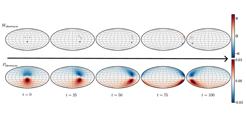
(a) The skew-Hermitian part (real component) of the vorticity and stream matrix at various time points, generated from skew-Hermitian initial data.

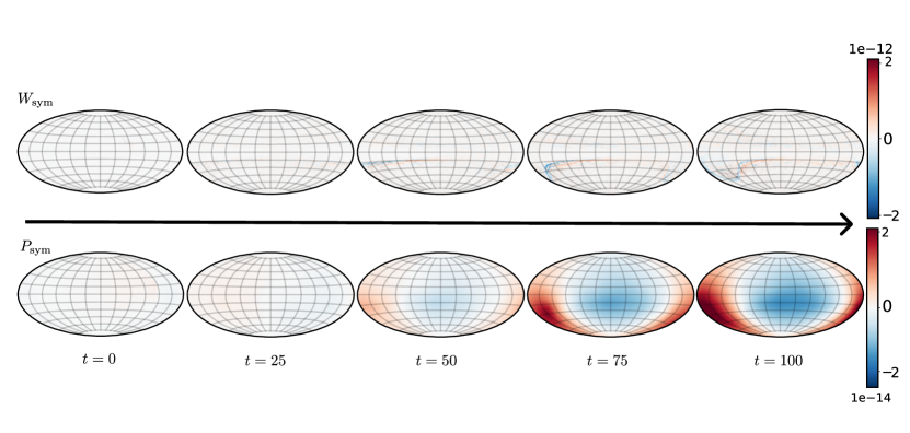
(b) The Hermitian part (imaginary component) of the vorticity and stream matrix at various time points, generated from skew-Hermitian initial data.

Figure 1. Evolution of the vorticity and stream matrices in a simulation of the EPDiff–Zeitlin system (19).

A natural question is what happens if the initial data is entirely Hermitian (imaginary), rather than skew-Hermitian (real). We can easily test this by taking instead the initial data to be $W_{0}=iB_{1}+iB_{2}-iB_{3}$. The resulting dynamics is then strikingly different. Indeed, as seen in Figure 2 (real component) and Figure 3 (imaginary component), instead of traversing and rotating about each other, the blobs deform and then collide in a complicated manner at about $T=60$. At this stage, the $L^{\infty}$-norm quickly grows, as seen at $T=78$. The situation is better understood in terms of the stream matrix $P_{n}$, seen in Figure 4 (real component) and Figure 5 (imaginary component). As the velocity field is given by the gradient of the stream function, we see that fluid particles below and above the equator are on collision trajectories, which eventually, at about $T=60$, leads to a complicated configuration that now also includes a significant amount of swirling motion (corresponding to the real component of the stream matrix $P_{n}$). The behavior is reminiscent of the “convergence to soliton solutions”, occurring in the Camassa–Holm equation (Camassa and Holm, 1993), which is the EPDiff equation in one dimension, and also observed numerically for “soliton filaments” in the two-dimensional EPDiff equation (Holm and Staley, 2013; Larsson et al., 2016).

(a) $T=0$

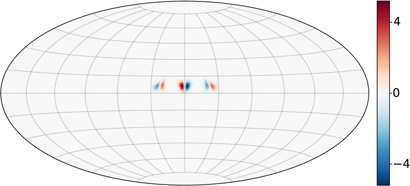
(b) $T=30$

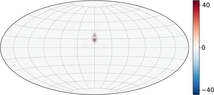
(c) $T=60$

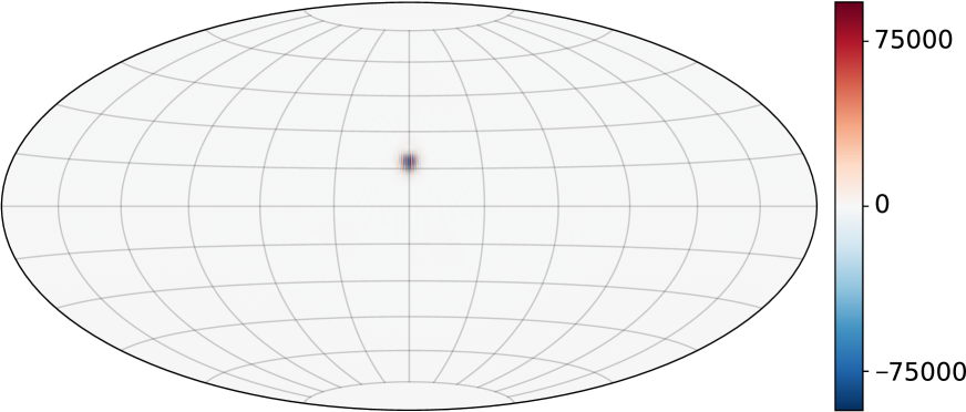
(d) $T=78$

Figure 2. The skew-Hermitian part (real component) of the vorticity matrix in the second simulation. Note that, while the component is initially $0$, it grows rapidly to about the same magnitude as the imaginary component.

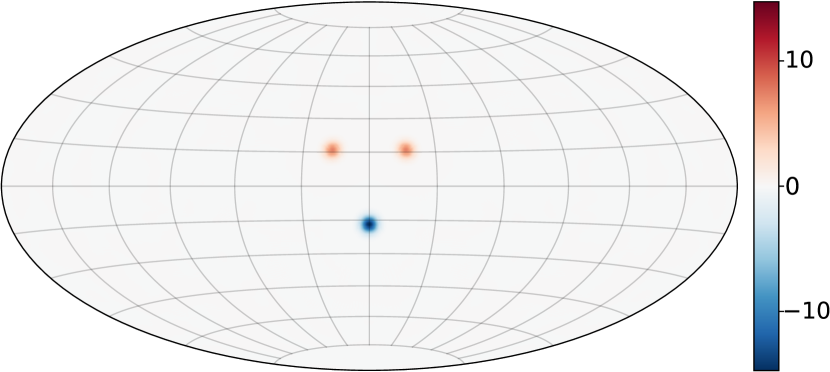
(a) $T=0$

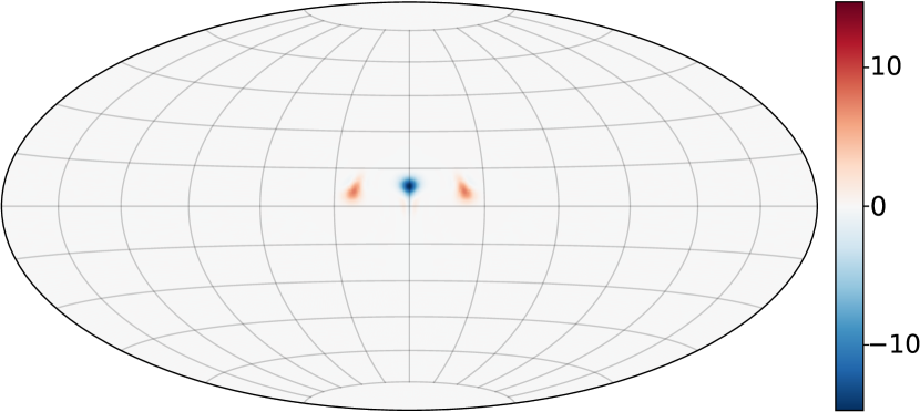
(b) $T=30$

(c) $T=60$

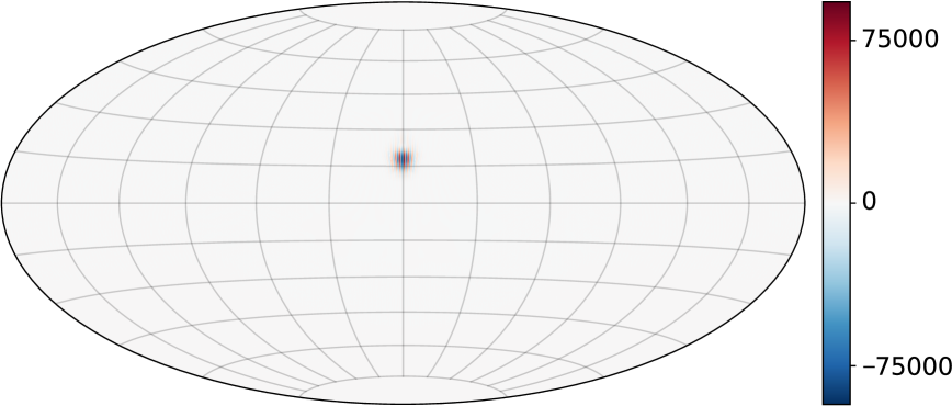
(d) $T=78$

Figure 3. The Hermitian part (imaginary component) of the vorticity matrix in the second simulation. The max-norm of the component is growing rapidly.

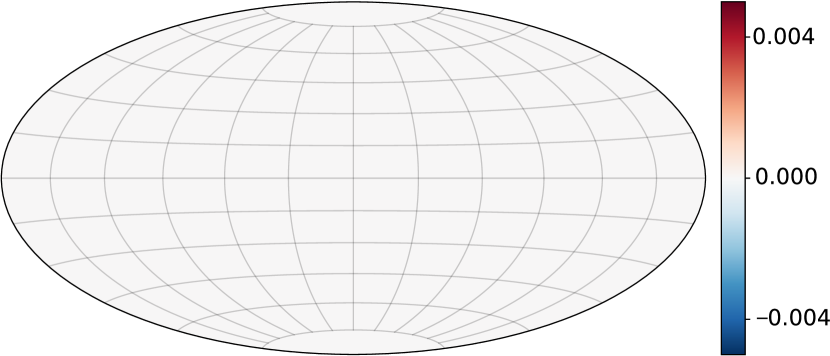
(a) $T=0$

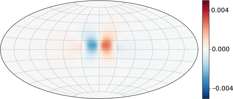
(b) $T=30$

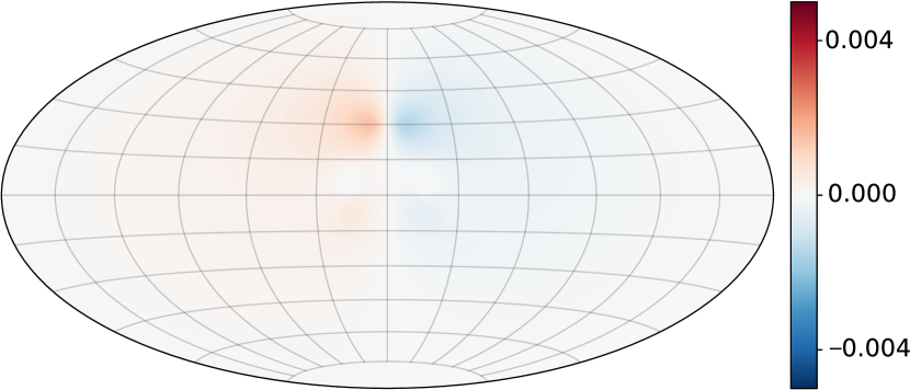
(c) $T=60$

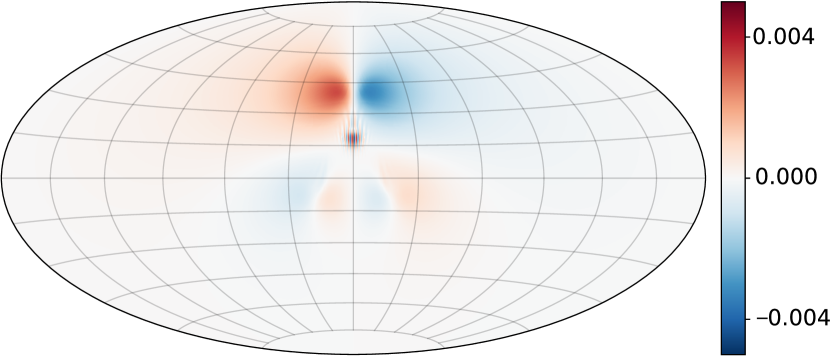
(d) $T=78$

Figure 4. The skew-Hermitian part (real component) of the stream matrix in the second simulation.

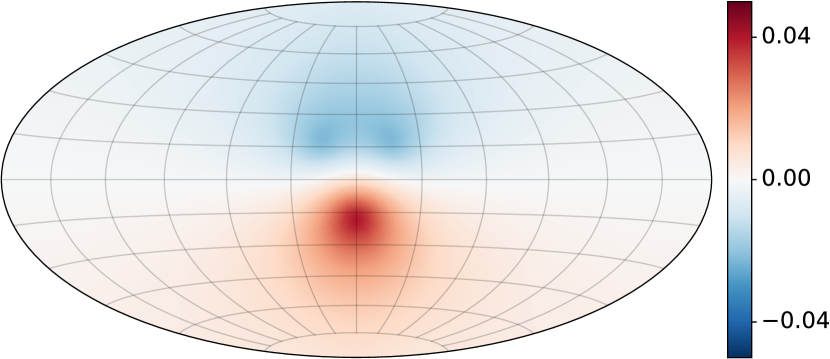
(a) $T=0$

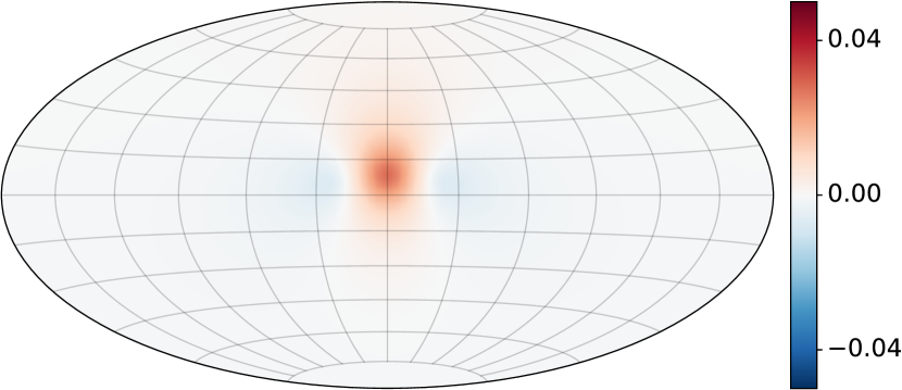
(b) $T=30$

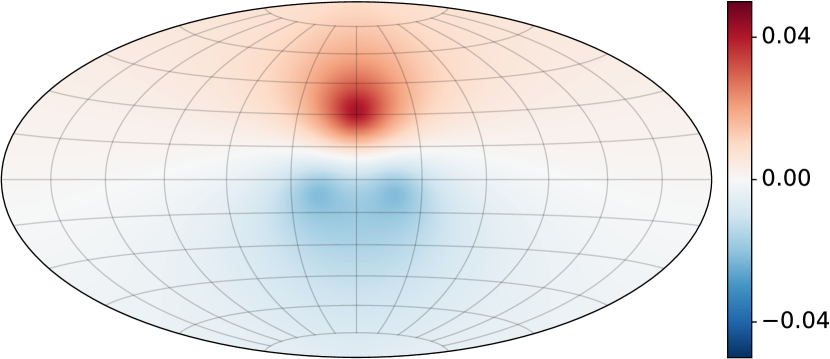
(c) $T=60$

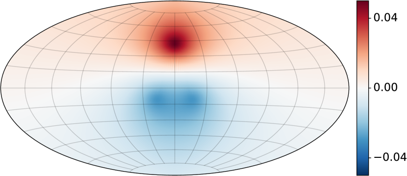
(d) $T=78$

Figure 5. The Hermitian part (imaginary component) of the stream matrix in the second simulation.

On a general note, compressible fluid equations are known to frequently exhibit “blow-up like” behavior, not observed for incompressible flows, unless there is a sufficiently strong potential to suppress the compressibility, as in the work of Ebin (1975). In particular, the 2-D barotropic compressible Euler equations may exhibit formations of singularities, as discussed by Sideris (1997). As the EPDiff equation lacks a counter-acting potential altogether, it may therefore exhibit effects such as formation solitions, sheets, and other singular solutions, as discussed by Holm and Marsden (2005). We stress that this is not an issue for the EPDiff equation in the context of shape analysis, since there, only solutions on short time intervals are of interest.

A possible use of the numerical method presented in this paper is to guide a theoretical study on the spherical EPDiff equation. In particular, blow-up of the EPDiff equation has been studied in dimensions higher than or equal to three (Bauer et al., 2023), but the two-dimensional case remains an interesting avenue for future research. Note that if $k$ is large enough, then it is easy to prove global existence of regular solution via the framework of Ebin and Marsden (1970). In particular, $k>2$ is enough for the EPDiff equation on $\amsmathbb{S}^{2}$, and for such global solutions the vector field of to remain bounded in the Sobolev $H^{k}$-norm. Even so, the complex vorticity field $\omega$ in Equation 15 may, and probably does, grow fast in the $L^{\infty}$-norm.

5. Outlook: a zoo of compressible Zeitlin models

This paper establishes the foundation for how to extend Zeitlin’s approach from incompressible to compressible fluid-type equations. It thereby enables an array of next directions and applications, in addition to the already showcased EPDiff equations. The most immediate ones are listed here, but shall be detailed in future work.

Barotropic Euler equations

There is an extension of Arnold’s description from incompressible to compressible fluids (see survey by Khesin et al. (2020)). This extension corresponds to replacing the group of volume-preserving diffeomorphisms with all diffeomorphisms. Thus, the geometric discretization of compressible fluids, particularly the barotropic Euler equation, can be addressed with the technique developed in this paper. For compressible fluids, one typically needs, in addition to the right-invariant Riemannian metric, a potential functional.

Geophysical shallow water equations

The sphere is, of course, an important fluid domain in geophysical contexts. Adaptations of Zeitlin’s model on the sphere to geophysically relevant settings, in particular the quasi-geostrophic model for planetary flows, are given by Franken et al. (2023). These equations are still incompressible, but there are other, more detailed geophysical models, such as the one-layer global shallow-water model of the atmosphere, where the dynamics is compressible. The developments in this paper enable Zeitlin’s approach as well for those equations.

Optimal mass transport

Optimal mass transport is closely related to compressible fluids via Otto calculus (Benamou and Brenier, 2000; Otto, 2001). It is natural to use the complexified framework presented here to develop a Zeitlin model of optimal mass transport, such that the transport maps are replaced by group elements in $\mathrm{PGL}(N,\amsmathbb{C})$. To this end, one needs a quantized analog of probability densities $\operatorname{Dens}(\amsmathbb{S}^{2})$. We achieve this via the result of Moser (1965) that $\operatorname{Dens}(\amsmathbb{S}^{2})\simeq\operatorname{Diff}(\amsmathbb{S}^{2})/\operatorname{Diff}_{\Omega}(\amsmathbb{S}^{2})$. Indeed, this gives quantized densities as $\mathrm{PGL}(N,\amsmathbb{C})/\mathrm{PU}(N)$, in turn equivalent to Hermitian matrices via polar factorization. Thus, we obtain a complexified version of the principal bundle picture advocated in the different, but also finite-dimensional, optimal transport context of Gaussian measures (Modin, 2017).

Diffeomorphic density matching

A possible use case from the realm of shape matching is the problem of finding an optimal diffeomorphism that transforms one initial density to a target density. This in turn could have potential uses in sampling (Bauer et al., 2017), computer graphics (Dominitz and Tannenbaum, 2010) and medical image analysis (Gorbunova et al., 2012; Haker et al., 2004; Rottman et al., 2015).

An approach to the inexact density matching problem suggested in Bauer et al. (2015) is as follows: given two densities

$$\rho_{0},\rho_{1}\in\operatorname{Dens}(\amsmathbb{S}^{2})\coloneqq\left\{\rho\in C^{\infty}(\amsmathbb{S}^{2},\amsmathbb{R})\mid\rho>0,\int_{\amsmathbb{S}^{2}}\rho\,\Omega=1\right\},$$

the problem consists of finding a diffeomorphism $\varphi\in\operatorname{Diff}(\amsmathbb{S}^{2})$ that warps, via pushforward of densities, $\rho_{0}$ to $\rho_{1}$.

The diffeomorphism $\varphi$ is given as the endpoint of a curve $\gamma(t)\in\operatorname{Diff}(\amsmathbb{S}^{2})$ that minimizes the inexact matching energy functional

(21) $$E(\varphi)=\int_{\amsmathbb{S}^{2}}|\varphi_{*}\rho_{0}-\rho_{1}|^{2}\,\Omega+\int_{\amsmathbb{S}^{2}}v\cdot Lv\,\Omega$$

where $v=\dot{\gamma}\circ\gamma^{-1}$ and $L=(1-\alpha\Delta)^{k}$ for some $k\in\amsmathbb{N}\cup\{0\}$ and $\alpha>0$. Here, $\Delta$ denotes the Laplace–Beltrami operator on vector fields.

The first term of $E(\varphi)$ is a similarity measure, penalizing dissimilarity between $\varphi_{*}\rho_{0}$ and $\rho_{1}$. The second term is a regularization that penalizes irregular transformations. This setting is called large diffeomorphic metric mapping (cf. Bruveris and Holm (2013) for an overview), but here in the context of densities instead of functions.

The matching problem admits a dynamical formulation for which the Euler–Arnold framework applies: the optimal, time-dependent velocity $v$ must fulfill the EPDiff equation (4) above. Thus, the EPDiff-Zeitlin equations (19), together with the time-discretization considered above, provide a geometric discretization of the inexact density matching problem just outlined.

References

- Arnold (1966) V. I. Arnold, Sur la géométrie différentielle des groupes de Lie de dimension infinie et ses applications à l’hydrodynamique des fluides parfaits, Ann. de l’Institut Fourier 16 (1966), 319–361.
- Arnold and Khesin (1998) V. I. Arnold and B. A. Khesin, Topological Methods in Hydrodynamics, Springer New York, 1998.
- Bauer et al. (2015) M. Bauer, S. Joshi, and K. Modin, Diffeomorphic density matching by optimal information transport, SIAM J. Imaging Sci. 8 (2015), 1718–1751.
- Bauer et al. (2017) M. Bauer, S. Joshi, and K. Modin, Diffeomorphic random sampling using optimal information transport, Lecture Notes in Computer Science, pp. 135–142, Springer International Publishing, 2017.
- Bauer et al. (2023) M. Bauer, S. C. Preston, and J. Valletta, Liouville comparison theory for blowup of Euler-Arnold equations, 2023.
- Benamou and Brenier (2000) J.-D. Benamou and Y. Brenier, A computational fluid mechanics solution to the Monge–Kantorovich mass transfer problem, Numer. Math. 84 (2000), 375–393.
- Bordemann et al. (1991) M. Bordemann, J. Hoppe, P. Schaller, and M. Schlichenmaier, and geometric quantization, Commun. Math. Phys. 138 (1991), 209–244.
- Bordemann et al. (1994) M. Bordemann, E. Meinrenken, and M. Schlichenmaier, Toeplitz quantization of Kähler manifolds and limits, Commun. Math. Phys. 165 (1994), 281–296.
- Bruveris and Holm (2013) M. Bruveris and D. D. Holm, Geometry of Image Registration: The Diffeomorphism Group and Momentum Maps, 2013, 1306.6854v2.
- Camassa and Holm (1993) R. Camassa and D. D. Holm, An integrable shallow water equation with peaked solitons, Phys. Rev. Lett. 71 (1993), 1661–1664.
- Cifani et al. (2023) P. Cifani, M. Viviani, and K. Modin, An efficient geometric method for incompressible hydrodynamics on the sphere, J. Comput. Phys. 473 (2023), 111772.
- da Silva (2008) A. C. da Silva, Lectures on Symplectic Geometry, Springer, 2008.
- Dominitz and Tannenbaum (2010) A. Dominitz and A. Tannenbaum, Texture mapping via optimal mass transport, IEEE Trans. Vis. Comput. Graph. 16 (2010), 419–433.
- Ebin (1975) D. G. Ebin, Motion of a slightly compressible fluid, Proc. Natl. Acad. Sci. U.S.A. 72 (1975), 539–542.
- Ebin and Marsden (1970) D. G. Ebin and J. E. Marsden, Groups of diffeomorphisms and the notion of an incompressible fluid., Ann. of Math. 92 (1970), 102–163.
- Engø and Faltinsen (2001) K. Engø and S. Faltinsen, Numerical integration of Lie–Poisson systems while preserving coadjoint orbits and energy, SIAM J. Numer. Anal. 39 (2001), 128–145.
- Franken et al. (2023) A. Franken, M. Caliaro, P. Cifani, and B. Geurts, Zeitlin truncation of a shallow water quasi-geostrophic model for planetary flow, 2023, 2306.15481.
- Gallagher (2002) I. Gallagher, Mathematical analysis of a structure-preserving approximation of the bidimensional vorticity equation, Num. Math. 91 (2002), 223–236.
- Gorbunova et al. (2012) V. Gorbunova, J. Sporring, P. Lo, M. Loeve, H. A. Tiddens, M. Nielsen, A. Dirksen, and M. de Bruijne, Mass preserving image registration for lung CT, Med. Image Anal. 16 (2012), 786–795.
- Hairer et al. (2006) E. Hairer, G. Wanner, and C. Lubich, Geometric Numerical Integration, Springer, 2006.
- Haker et al. (2004) S. Haker, L. Zhu, A. Tannenbaum, and S. Angenent, Optimal mass transport for registration and warping, Int. J. Comput. Vis. 60 (2004), 225–240.
- Holm and Marsden (2005) D. D. Holm and J. E. Marsden, Momentum maps and measure-valued solutions (peakons, filaments, and sheets) for the EPDiff equation, pp. 203–235, Birkhäuser Boston, Boston, MA, 2005.
- Holm and Staley (2013) D. D. Holm and M. F. Staley, Interaction dynamics of singular wave fronts, 2013.
- Hoppe (1989) J. Hoppe, Diffeomorphism groups, quantization, and , Int. J. Mod. Phys. A 04 (1989), 5235–5248.
- Hoppe and Yau (1998) J. Hoppe and S.-T. Yau, Some properties of matrix harmonics on , Commun. Math. Phys. 195 (1998), 67–77.
- Khesin et al. (2020) B. Khesin, G. Misiołek, and K. Modin, Geometric hydrodynamics and infinite-dimensional Newton’s equations, Bull. Amer. Math. Soc. 58 (2020), 377–442.
- Larsson et al. (2016) S. Larsson, T. Matsuo, K. Modin, and M. Molteni, Discrete variational derivative methods for the EPDiff equation, 2016.
- Le Floch (2018) Y. Le Floch, A Brief Introduction to Berezin–Toeplitz Operators on Compact Kähler Manifolds, Springer International Publishing, 2018.
- Marsden and Ratiu (1999) J. E. Marsden and T. Ratiu, Introduction to Mechanics and Symmetry, Springer, 1999.
- Modin (2017) K. Modin, Geometry of matrix decompositions seen through optimal transport and information geometry, J. Geom. Mech. 9 (2017), 335–390.
- Modin and Perrot (2023) K. Modin and M. Perrot, Eulerian and Lagrangian stability in Zeitlin’s model of hydrodynamics, 2023.
- Modin and Viviani (2019) K. Modin and M. Viviani, Lie–Poisson methods for isospectral flows, Found. Comut. Math. 20 (2019), 889–921.
- Modin and Viviani (2020) K. Modin and M. Viviani, A Casimir preserving scheme for long-time simulation of spherical ideal hydrodynamics, J. Fluid Mech. 884 (2020).
- Moser (1965) J. Moser, On the volume elements on a manifold, Trans. Amer. Math. Soc. 120 (1965), 286–294.
- Mumford (1998) D. Mumford, Pattern theory and vision, Questions Mathématiques en Traitement du Signal et de L’Image, pp. 7–13, Institut Henri Poincaré, 1998.
- Otto (2001) F. Otto, The geometry of dissipative evolution equations: the porous medium equation, Comm. Partial Differential Equations 26 (2001), 101–174.
- Rottman et al. (2015) C. Rottman, M. Bauer, K. Modin, and S. Joshi, Weighted diffeomorphic density matching with applications to thoracic image registration, Proc. 5th MICCAI Workshop on Mathematical Foundations of Computational Anatomy (MFCA), Munich, Germany, 2015.
- Sideris (1997) T. C. Sideris, Delayed singularity formation in 2D compressible flow, Am. J. Math. 119 (1997), 371–422.
- Younes (2010) L. Younes, Shapes and Diffeomorphisms, Springer-Verlag, Berlin, 2010.
- Zeitlin (1991) V. Zeitlin, Finite-mode analogs of 2D ideal hydrodynamics: Coadjoint orbits and local canonical structure, Phys. D: Nonlinear Phenom. 49 (1991).
- Zeitlin (2004) V. Zeitlin, Self-consistent finite-mode approximations for the hydrodynamics of an incompressible fluid on nonrotating and rotating spheres, Phys. Rev. Lett. 93 (2004).