Zeitlin truncation of a Shallow Water Quasi-Geostrophic model for planetary flow

Abstract

In this work, we consider a Shallow-Water Quasi Geostrophic equation on the sphere, as a model for global large-scale atmospheric dynamics. This equation, recently studied by Verkley (2009) and Schubert et al. (2009), possesses a rich geometric structure, called Lie-Poisson, and admits an infinite number of conserved quantities, called Casimirs. In this paper, we develop a Casimir preserving numerical method for long-time simulations of this equation. The method develops in two steps: firstly, we construct an N-dimensional Lie-Poisson system that converges to the continuous one in the limit $N\to\infty$; secondly, we integrate in time the finite-dimensional system using an isospectral time integrator, developed by Modin and Viviani (2020). We demonstrate the efficacy of this computational method by simulating a flow on the entire sphere for different values of the Lamb parameter. We particularly focus on rotation-induced effects, such as the formation of jets. In agreement with shallow water models of the atmosphere, we observe the formation of robust latitudinal jets and a decrease in the zonal wind amplitude with latitude. Furthermore, spectra of the kinetic energy are computed as a point of reference for future studies.

1 Introduction

In the context of Geophysical Fluid Dynamics, Primitive equations (PE) are an accurate model governing the dynamics of large-scale oceanic and atmospheric motions. Due to their complexity, simplified models have been derived from them. The Rotating Shallow Water (RSW) equations on the sphere form an important example. In this case, the simplification is based on the disparity of horizontal and vertical scales. The equations are obtained by vertical averaging of the velocity field.

From the one-layer global shallow-water model of the atmosphere, a simplified equation has been independently derived by Verkley (2009) and Schubert et al. (2009), based on previous works of Charney and Stern (1962) and Kuo (1959). This equation, which we will refer to as the Balanced Shallow Water (BSW) equation, is derived from RSW by using a non-divergence assumption for the horizontal velocity field, together with a linear balance equation linking the stream function and the geopotential. This simplifying procedure leads to an equation for the potential vorticity that is identical in form to the rotating Euler equation for the relative vorticity, except for an additional $f^{2}$-dependent term, where $f$ is the Coriolis parameter. To validate the BSW model, Verkley considers the dynamics of linearized Rossby waves and shows that these waves accurately reproduce the westward-propagating waves of the second class of the original shallow-water equations, studied in Longuet-Higgins (1968). Moreover, the associated 2D turbulence is studied in Verkley and Lynch (2009) and in Schubert et al. (2009), where the anisotropic Rhines barrier is derived.
The geometric structure is a remarkable property that the BSW equation and the rotating Euler equations share. As we will show, both equations form a Lie-Poisson system and admit an infinite number of independent conserved quantities, called Casimirs.

The aim of the present work is to develop a structure-preserving numerical method, based on Zeitlin discretization, Zeitlin (1991, 2004), and on an isospectral time-integrator developed in Modin and Viviani (2020). This method was recently applied successfully to underpin Kraichnan’s double scaling hypothesis for 2D forced turbulence in Cifani et al. (2022) and is also adopted here. The combination of Zeitlin discretization and isospectral time-integration for flow on a sphere is shown to capture the double cascade in the kinetic energy spectrum as is typical for 2D turbulence, as well as the emergence of zonal jets across the sphere.

The organization of this paper is as follows. In Section II the mathematical model for BSW flow on a sphere is presented. Section III is devoted to the Zeitlin truncation and the Lie-Poisson time-integration method. An illustration of BSW flow on a rotating sphere is discussed in Section IV and concluding remarks are collected in Section V.

2 BSW equations on the sphere

The one-layer rotating shallow water equation on the sphere is a model that, under the assumptions of constant density and columnar motion, describes the motion of a thin layer of fluid on the surface of a rotating sphere. The fluid is described by a two-dimensional horizontal (or tangential) velocity field $\textbf{u}=(u,v)$ and a local height $h$. This system admits a materially conserved quantity called potential vorticity:

$$P:=\frac{\omega+f}{h}$$ (1)

where $\omega:=\hat{\mathbf{r}}\cdot(\nabla\times\mathbf{u})$ is the radial component of the relative vorticity and $f=2\Omega\sin\phi$ is the Coriolis parameter. Moreover, $\Omega$ denotes the angular velocity of the planet, and $\phi$ is the latitude.
Starting from the one-layer RSW equations on the sphere, Verkley (2009) and Schubert et al. (2009) derived the simplified BSW model, by adding three assumptions as follows:

Assumption 1: We denote the local height of the fluid column by

$$h(\mathbf{x},t)=H+\eta(\mathbf{x},t)+b(\mathbf{x})$$ (2)

where $H$ is a uniform average height and $\eta$ is a variable surface elevation. The quantity $b$ denotes the topography and in the following will be assumed to be zero ($b(\mathbf{x})=0$). The first assumption consists in assuming that the variable surface elevation is much smaller than the average height, i.e.,

$$\eta/H\ll 1$$ (3)

Assumption 2: Motivated by this first assumption and by the continuity equation for RSW, we assume that the divergence of the horizontal velocity can be approximated as zero. Using the Helmholtz decomposition, we write the horizontal velocity in terms of a stream function $\psi$ such that

$$\mathbf{u}=\hat{\textbf{r}}\times\nabla\psi.$$ (4)

Assumption 3: In order to derive a closed dynamical system from the material conservation of the potential vorticity (1), we propose a form of balance that relates the velocity field u to the local height $h$, or, equivalently to the geopotential $\varphi:=g\eta$, where $g$ is the gravitational acceleration. Among the linear balance relations, we choose the simplest one, which relates the stream function and the variable height as follows:

$$f\psi=g\eta.$$ (5)

This relation is inspired by quasi-geostrophic systems, in which there exists an approximate balance between the Coriolis force and pressure forces. It was first considered by Daley (1983), as a simplification of the balance relation $\nabla\cdot(-f\nabla\psi+g\nabla\eta)=0$ introduced by Lorenz (1960).

Using Assumptions 1, 2 and 3 we can derive the BSW system from the RSW point of reference. As we assume a small free surface elevation, an expansion up to first order in $\eta/H$ yields

$$\frac{1}{h}=\frac{1}{H}\left(1-\frac{\eta}{H}\right)$$ (6)

so that the potential vorticity becomes

$$P=\frac{\omega+f}{H}\left(1-\frac{\eta}{H}\right)$$ (7)

In the regime of rapid rotation, the dominant contribution to the potential vorticity according to Verkley (2009) reads

$$HP=\omega+f-\frac{\eta}{H}f=:q$$ (8)

defining the central dynamic variable $q$ to which we turn next. By using the linear balance relation (5) we write the potential vorticity $q$ as:

$$q=\omega+f-\frac{f^{2}}{gH}\psi$$ (9)

In this approximation, we can formulate the material conservation law for the potential vorticity (1) as

$$\frac{\partial q}{\partial t}+(\hat{\textbf{r}}\times\nabla\psi)\cdot\nabla q=0,$$ (10)

where

$$q=2\Omega\sin\phi+\Delta\psi-\frac{4\Omega^{2}}{gH}\sin^{2}\phi\psi$$ (11)

Equations (10) and (11) are the central formulation of the BSW model on the sphere. Anticipating the Zeitlin truncation (Zeitlin (2004)) in the next section, we non-dimensionalize the equations using the radius of the sphere $R$ as the length scale, and $\Omega^{-1}$ as the time scale, which allows us to rewrite the model as follows

$$\begin{cases}\dot{q}=\left\{\psi,q\right\}\\ \left(\Delta-\gamma\mu^{2}\right)\psi=q-2\mu,\end{cases}$$ (12)

where $\mu=\sin{\phi}$ and $\{\cdot,\cdot\}$ is the Poisson bracket on the unit sphere, which in the latitude-longitude coordinate system reads as

$$\{\psi,q\}=\frac{1}{\cos\phi}\left(\frac{\partial\psi}{\partial\phi}\frac{\partial q}{\partial\theta}-\frac{\partial\psi}{\partial\theta}\frac{\partial q}{\partial\phi}\right).$$ (13)

Moreover, $\gamma$ is Lamb’s parameter, which expresses the ratio between the radius of the sphere, and the typical size of quasi-geostrophic vortices (Vallis (2019)) given by the Rossby deformation length $R_{d}$:

$$\gamma=4\frac{R^{2}}{R_{d}^{2}},\quad\mbox{where}\quad R_{d}=\frac{\sqrt{gH}}{\Omega}$$ (14)

Equations (12) constitute an infinite dimensional Lie–Poisson system on the space of smooth functions on the sphere $C^{\infty}(\mathbf{S}^{2})$ (Arnol’d and Khesin (1992)). It has Hamiltonian

$$H(q)=\frac{1}{2}\int_{\mathbf{S}^{2}}(q-f)\psi\,\mbox{d}x$$ (15)

and admits an infinite number of conserved quantities called Casimirs. In fact, for any $g\in C^{\infty}(\mathbf{R})$, the quantities

$$\mathcal{C}(q)=\int_{\mathbf{S}^{2}}g(q)\,\mbox{d}x$$ (16)

can be readily verified to be independent of time, which is a striking aspect of the dynamics of the BSW model.

The existence of an infinite family of conserved quantities is a remarkable property. While most numerical methods for Poisson equations are constructed such that the discretization of the Hamiltonian is conserved, here, we aim to conserve a subset of the infinite family of Casimirs. In the next section, we will derive a special finite-dimensional truncation of equations (12) that preserves all Casimirs of the discrete model.

3 Numerical method for Zeitlin truncation

In this section, we follow the approach by Zeitlin to construct a numerical scheme with which the geometric structure of the BSW equations can be preserved optimally – this procedure is sometimes referred to as ‘quantization’, contrasting the familiar ‘discretization’. Specifically, we show how to construct and integrate a finite-dimensional analogue of equations (12) while preserving all the associated independent Casimirs.

3.1 Finite truncation of the Poisson bracket

We begin our construction of the Casimir-preserving numerical method by constructing a finite-dimensional analogue of (12). This will be referred to as the Zeitlin truncation. Fundamental to the derivation, we notice that the couple $(C^{\infty}(\mathbf{S}^{2}),\{\cdot,\cdot\})$ forms an infinite dimensional Lie algebra and the existence of Casimirs is a direct result of this Lie-Poisson structure. Therefore, following Zeitlin, we look for a sequence of N-dimensional Lie algebras $(\mathbf{g}_{N},[\cdot,\cdot]_{N})$ that constitute an approximation, in a sense specified later, of $(C^{\infty}(\mathbf{S}^{2}),\{\cdot,\cdot\})$ in the limit $N\to\infty$. Here, $\mathbf{g}_{N},$ denotes an N-dimensional vector space and $[\cdot,\cdot]_{N}$ refers to the bilinear form of the Lie algebra. The family of finite-dimensional Lie algebras $(\mathbf{g}_{N},[\cdot,\cdot]_{N})$ is referred to as $L_{N}$-approximation (Bordemann et al. (1991)).

In Bordemann et al. (1994), it is shown that the $L_{N}$-approximation for $(C^{\infty}(\mathbf{S}^{2}),\{\cdot,\cdot\})$ can be obtained using the Lie algebra $(\mathfrak{gl}(N),[\cdot,\cdot])$, where $\mathfrak{gl}(N)$ is the set of complex $N\times N$ matrices and $[\cdot,\cdot]$ is the matrix commutator. Indeed, we can construct a surjective projection $\Pi_{N}:C^{\infty}(\mathbf{S}^{2})\to\mathfrak{gl}(N)$ such that

• $\Pi_{N}f-\Pi_{N}g\to 0$ as $N\to\infty$ implies $f=g$;

• $\Pi_{N}\{f,g\}=\frac{N^{3/2}}{\sqrt{16\pi}}[\Pi_{N}f,\Pi_{N}g]+O(1/N^{2})$

Using this projection, we can associate with every smooth function on $\mathbf{S}^{2}$ a matrix in $\mathfrak{gl}(N)$. The action of the projection $\Pi_{N}$ is linear and explicitly known: to each spherical harmonics $Y_{l,m}\in C^{\infty}(\mathbf{S}^{2})$ we associate a matrix $i\widehat{T}_{l,m}\in\mathfrak{gl}(N)$. Here $i$ is the imaginary unit and the explicit expression of the matrices $\widehat{T}_{l,m}$ is reported in Appendix A. Thus, using the spherical harmonics as a basis, we associate with any function given by

$$q=\sum_{l=0}^{\infty}\sum_{m=-l}^{l}q_{l,m}Y_{l,m}\in C^{\infty}(\mathbf{S}^{2})$$ (17)

the matrix

$$Q:=\Pi_{N}q=\sum_{l=0}^{N-1}\sum_{m=-l}^{l}iq_{l,m}\widehat{T}_{l,m}^{N}.$$ (18)

Notice that for a real-valued function $q$, the spherical harmonics coefficients satisfy $q_{l,m}=(-1)^{m}q_{l,-m}$. This translates to the matrix condition $Q+Q^{\dagger}=0$, where $Q^{\dagger}$ is the conjugate transpose of $Q$. For this reason, we can restrict to the subalgebra of skew-Hermitian matrices $Q\in\mathfrak{u}(N)\subset\mathfrak{gl}(N)$. For convenience, we, therefore, define the modified basis $T_{lm}$ and find

$$Q=\sum_{l=0}^{N-1}\sum_{m=-l}^{l}q_{l,m}T_{l,m}^{N}$$ (19)

where

$$T_{l,m}^{N}=\frac{i}{\sqrt{2}}\left(\widehat{T}_{l,m}^{N}+(-1)^{m}\widehat{T}_{l,-m}^{N}\right)\quad\mbox{for}\,\,m>0$$

$$T_{l,-m}^{N}=\frac{1}{\sqrt{2}}\left(\widehat{T}_{l,-m}^{N}-(-1)^{m}\widehat{T}_{l,m}^{N}\right)\quad\mbox{for}\,\,m>0$$

$$T_{l,0}^{N}=i\widehat{T}_{l,0}^{N}\quad\mbox{for}\,\,m=0$$

In terms of the discrete basis, our system of equations (12) takes the following form:

$$\begin{cases}\dot{Q}=\left[Q,P\right]_{N}\\ \Delta_{N}P-\gamma\Pi_{N}(\mu^{2}\psi)=Q-2\Pi_{N}\mu,\end{cases}$$ (20)

where $Q$ is usually referred to as the potential vorticity matrix and $P$ as the stream matrix. We use the scaled commutator $[\cdot,\cdot]_{N}=N^{3/2}/\sqrt{16\pi}[\cdot,\cdot]$ as given by the aforementioned projection of the Poisson bracket (Modin and Viviani (2020)). Here $\Delta_{N}$ is the quantized Laplace-Beltrami operator, that satisfies $\Delta_{N}\widehat{T}_{l,m}=-l(l+1)\widehat{T}_{l,m}$, as further detailed in appendix A.

3.2 Computation of the stream function

The scheme presented in equations (20) involves computation of the stream matrix $P$. Determining the stream matrix involves quantizing the functions $\mu$ and $\mu^{2}\psi$. For the projection of the former, we use the expansion in terms of spherical harmonics:

$$\mu=\sin\phi=2\sqrt{\frac{\pi}{3}}Y_{1}^{0}.$$ (21)

The discrete representation is therefore given by the following projection:

$$M:=\Pi_{N}\mu=2i\sqrt{\frac{\pi}{3}}\widehat{T}_{1,0},$$ (22)

which can be calculated explicitly. The term $\mu^{2}\psi$ is more involved, as it requires the projection of a product of functions. In appendix B, we discuss a method for approximating the projection of a product of two functions on the sphere, together with its accuracy. In practice, given two real functions $f$ and $g$ and their associated elements of $\mathfrak{u}(N)$ given by $F=\Pi_{N}f$ and $G=\Pi_{N}g$, we use the following approximation:

$$\Pi_{N}(fg)\approx-\frac{i}{2}\sqrt{\frac{N}{4\pi}}(FG+GF),$$ (23)

which associates multiplication with the anti-commutator on $\mathfrak{u}(N)$. In our specific case, using the expansion:

$$\sin^{2}\phi=\frac{2}{3}\sqrt{\pi}Y_{0}^{0}+\frac{4}{3}\sqrt{\frac{\pi}{5}}Y_{2}^{0},$$ (24)

we can define

$$S:=\Pi_{N}\mu^{2}=\frac{2i}{3}\sqrt{\pi}\widehat{T}_{0,0}^{N}+\frac{4i}{3}\sqrt{\frac{\pi}{5}}\widehat{T}_{2,0}^{N}.$$ (25)

which enables writing:

$$\Pi_{N}(\mu^{2}\psi)\approx-\frac{i}{2}\sqrt{\frac{N}{4\pi}}(SP+PS).$$ (26)

The final step which allows us to solve the system for $P$ is the observation that the matrix harmonics $\widehat{T}_{l,0}^{N}$ only have non-zero entries on the diagonal (see appendix A). If we denote the diagonal of $S$ as the vector $s\in\mathbb{C}^{N}$ such that $s_{i}=S_{ii}$, we can write:

$$\Pi_{N}(\mu^{2}\psi)\approx\tilde{S}\circ P,\quad\mbox{where}\quad\tilde{S}_{ij}=-\frac{i}{2}\sqrt{\frac{N}{4\pi}}(s_{i}+s_{j})$$ (27)

where $\circ$ is the Hadamard, or entry-wise product.

Finally, we arrive at the discrete system by substituting the above results into equations 20:

$$\begin{cases}\dot{Q}=\left[Q,P\right]_{N}\\ \Delta_{N}P-\gamma\tilde{S}\circ P=Q-2M\end{cases}$$ (28)

where the matrices $M$ and $\tilde{S}$ are defined in equations (22) and (27) respectively. The equation for $P$ can be solved efficiently using a clever splitting of the problem along diagonals of the matrix $P$. The implementation is based on the methodology used by Cifani et al. (2023), and is further detailed in appendix C.

The time-evolution of $Q$ in equation (28) is isospectral since the spectrum of the matrix is preserved by the matrix commutator (Viviani (2019)). This implies that traces of powers of the quantized potential vorticity are conserved. In other words, the quantities

$$C_{k}(W)=\mbox{Tr}(Q^{k})\ \ \text{for}\ \ k=1,2,...,N$$ (29)

are conserved by (28). This represents the discrete analogue of the conserved Casimirs (Cifani et al. (2023)) in (16).
Additionally, the system is Lie-Poisson with the Hamiltonian $H_{N}$ given by:

$$H_{N}=\frac{1}{2}\mbox{Tr}\left(P(Q-2M)^{\dagger}\right)$$ (30)

System (28) provides a finite-dimensional analogue of equations (12), relating the potential vorticity matrix to the stream matrix. In the next section, we integrate (28) by means of an isospectral time integrator that preserves all the Casimirs (29).

3.3 Isospectral time-integration

In order to preserve the discrete Casimirs (29), we use an isospectral Lie-Poisson time-integrator following Modin and Viviani (2020). This retains the basic discrete Lie-Poisson dynamics. The time integrator is based on the implicit midpoint rule and can be written as follows:

$$\begin{cases}\tilde{Q}=Q_{n}+\frac{h}{2}[P,\tilde{Q}]_{N}+\frac{h^{2}}{4}P\tilde{Q}P\\ Q_{n+1}=\tilde{Q}+\frac{h}{2}[\tilde{P},\tilde{Q}]_{N}-\frac{h^{2}}{4}\tilde{P}\tilde{Q}\tilde{P}\end{cases}$$ (31)

The first equation is solved for $\tilde{Q}$ using fixed point iteration that creates a sequence $\{\tilde{Q}_{k}\}$, with $\tilde{Q}_{0}=Q_{n}$, which converges to $\tilde{Q}$ as $k\rightarrow\infty$. This contraction was found to yield rapid convergence and only a small number of iterations was found necessary to reach a set tolerance. In test calculations we may typically reach an $L_{\infty}$-norm of $\tilde{Q}_{k+1}-\tilde{Q}_{k}$ of $O(10^{-12})$ after only $3$ iterations. To complete a time-step, the sufficiently converged approximation $\tilde{Q}_{K}$ of $\tilde{Q}$ for suitable $K$ is used once again to evaluate the full right-hand side in the second equation in (31).

4 Simulation of zonal jet formation

To illustrate the Zeitlin truncated BSW model with Casimir-preserving iso-spectral time-integration, we simulate a particular rotating sphere case. Results obtained using the BSW equation will be compared with findings based on the Navier-Stokes equations on a rotating sphere from Cifani et al. (2022). Therefore, we consider the BSW equation with additional forcing, dissipation and (Rayleigh) friction:

$$\begin{cases}\dot{q}=\left\{\psi,q\right\}+\nu(\Delta q+2q)-\alpha q+F,\\ \left(\Delta-\gamma\mu^{2}\right)\psi=q-2\mu,\end{cases}$$ (32)

where $\nu$ is the dimensionless viscosity, $F$ is the forcing and $\alpha q$ is the dimensionless Rayleigh friction to avoid an accumulation of energy at large scales due to the inverse energy cascade in 2D turbulence. Moreover, $2\nu q$ arises from the spherical geometry (Lindborg and Nordmark (2022)). Following Cifani et al. (2022), the forcing is time-dependent, derived from a Wiener process uncorrelated to the time scales of the flow. The forcing is localized in a narrow band in spherical harmonic space around degree $l_{f}=100$.

The viscous dissipation, damping and forcing are integrated using a second-order Crank-Nicolson scheme, while the isospectral integrator is used for the convective term. This ensures that the solution departs from the level sets of the Casimirs only due to the non-conservative terms in the equation and not by numerical inaccuracies in the discretization of convection. By denoting with $\Phi_{iso,h}$ the isospectral map for convection and by $\Phi_{CN,h}$ the Crank-Nicolson map for the remaining terms on a time interval $h$, the time integration is obtained using the second-order Strang splitting:

$$Q^{n+1}=\left(\Phi_{CN,h/2}\circ\Phi_{iso,h}\circ\Phi_{CN,h/2}\right)Q^{n},$$ (33)

where $h$ is the time step and $n$ the time level.

In the following, we report the flow generated at different values of Lamb’s parameter $\gamma$. In order to appreciate the qualitative changes in the flow, we chose to display three cases: $\gamma=0$ (which corresponds to the limit $R_{d}\to\infty$ in which we recover the two-dimensional Navier-Stokes equations), $\gamma=10^{3}$ and $\gamma=10^{4}$.

Figures 1 shows a snapshot of the zonal component of the velocity field at a time at which the flow is in a statistically stationary state for each choice of parameter $\gamma$. The spatial resolution is set to $N=2048$, which was found to accurately represent the smallest scales in the flow.

As a reference, we consider the solution obtained at $\gamma=0$ as shown in the left snapshot of Figure 1. The solution displays a clear zonal structure, with the formation of a large number of zonal jets. In particular, we notice how these jets appear to have an intensity that is quite independent of the latitude. The situation is different when we solve the BSW equation at $\gamma_{1}=10^{3}$ (middle snapshot in Fig. 1). Here, we see that while the number of zonal jets appears unaffected, there is an apparent graded intensity of the jets which ranges from comparably weak jets near the poles to strong jets near the equator. This trend is even stronger when Lamb’s parameter is increased to $\gamma=10^{4}$ (right shapshot in Fig. 1), which corresponds to a smaller Rossby deformation length. This effect is illustrated quantitatively in Figure 2, where the zonal velocity, averaged along longitudes, is displayed as a function of latitude. Here we clearly see how the width and intensity of jets near the equator are almost unaffected by the change in the Lamb parameter. However, we observe that the intensity of jets close to the poles gets attenuated strongly with increasing $\gamma$. This phenomenon of jet attenuation was already observed by Scott and Polvani (2006), who simulated the RSW equations on the sphere in order to study the atmospheric circulation of giant planets. This observation indicates that the fundamental physical property of equatorial confinement of zonal jets with the decrease of the Rossby deformation length is encoded in the BSW model.

In Figure 3 we show the kinetic energy spectrum for the three values of Lamb’s parameter, in terms of the degree $l$ of the spherical harmonics. The spectra have been split into the zonal ($m=0$) and the non-zonal ($m\neq 0$) energy contributions. First of all, we notice how, in all spectra, the non-zonal energy undergoes a double cascade, with a slope of $-5/3$ towards large scales and of $-3$ towards small scales, as expected for 2D turbulence on the sphere (Lindborg and Nordmark (2022)). This double cascade was also reported recently for isotropic turbulence in Cifani et al. (2022). Also, we notice how the most energetic large-scale modes come from the zonal contribution, with a peak around $l=20$ for all three cases.

As we increase the value of $\gamma$, we observe two trends in the kinetic energy spectra which relate to the phenomenon of equatorial confinement of zonal jets. First, we notice that, while the degree $l$ of the peak in the energy spectrum of the zonal modes appears unaffected by $\gamma$, the energy contained in these modes clearly diminishes as $\gamma$ grows. Second, in the case where $\gamma=0$, we notice that there is a rapid decay in the energy of the non-zonal modes as we move towards low wavenumbers $l$. This effect is known as the anisotropic Rhines barrier effect (Rhines (1975)), and it is believed to be responsible for the formation of zonal jets (Vallis and Maltrud (1993)). This effect takes place at low wavenumbers $l$ with $m\neq 0$, i.e. in the spectral region where the flow is dominated by waves rather than turbulence (Huang and Robinson (1998)). When $\gamma\neq 0$, the decay of energy in non-zonal modes becomes less rapid, i.e., they contain more energy than their counterparts at $\gamma=0$. As a consequence, even if at low wavenumbers the spectrum is still dominated by zonal modes, the non-zonal modes at low $l$ become important when $\gamma\neq 0$.

We notice that a similar phenomenon has been studied in the works of Theiss (2004, 2006). In the first of these works, a generalized quasi-geostrophic equation that allows a latitude-dependent Rossby deformation length is considered. Similarly to what we find in our simulations of the BSW model, they show an equatorial confinement of zonal jets, together with an attenuation of the Rhines barrier, which can be bypassed at certain latitudes. In the BSW model, in fact, the effect of a variable Rossby deformation length is naturally encoded in the factor $\gamma\mu^{2}$ in (12). For this reason, we believe that the numerical method, here developed, for the solution of the BSW equation will be instrumental to further the understanding of geostrophic turbulence, a thorough investigation of which is left for future work.

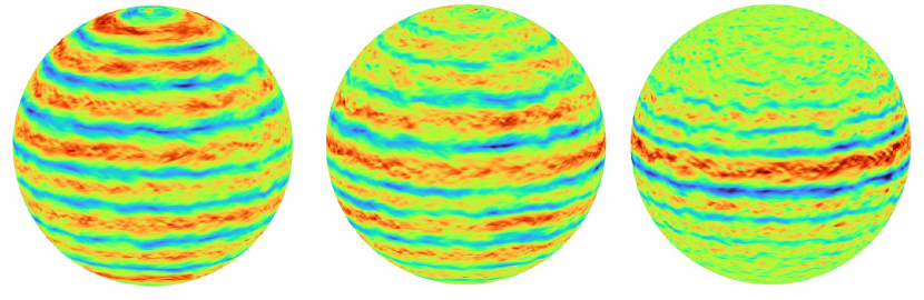
Figure 1: Zonal velocity of statistically stationary BSW flow at $\gamma=0$ (left), $\gamma=10^{3}$ (middle) and $\gamma=10^{4}$ (right). The colour scale is the same in each simulation and ranges between blue and red, representing clockwise and anti-clockwise motion respectively

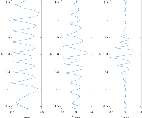
Figure 2: Mean zonal velocity profiles averaged over longitude as a function of latitude for the NS flow (a) and simulations of the BSW equation at $\gamma=10^{3}$ (b) and $\gamma=10^{4}$ (c).

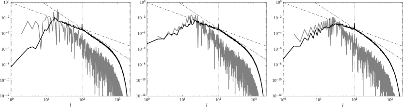
Figure 3: Kinetic energy spectra for the cases $\gamma=0$ (left), $\gamma=10^{3}$ (middle) and $\gamma=10^{4}$ (right). The spectra are shown as a function of the spherical harmonics number $l$, split into the zonal modes ($m=0$) in gray, and the non-zonal modes ($m\neq 0$) in black. For reference, the Kraichnan scalings $-5/3$ and $-3$ are shown. The dotted vertical line indicates the modes at which the forcing is centered.

5 Conclusions

In this work, we developed a Casimir preserving numerical method for the BSW system (12), and we used it to simulate the BSW flow on the sphere at different values of the Lamb’s parameter $\gamma$. As we observed in Section 4, the BSW model displays key features which are characteristic of rotating shallow water equations, such as the formation of robust zonal jets and the decrease of the zonal wind amplitude with latitude (Scott and Polvani (2006)). These fundamental physical mechanisms, while hidden in the more complex rotating shallow water model, are here clearly linked to the appearance of the parameter $\gamma$ in the operator relating stream function and vorticity. Moreover, by solving the governing equations on the sphere one can account fully account for latitude-dependent effects without having to resort to typical approximations on local tangent planes. We, therefore, expect this tool to be valuable in deepening the current understanding of geostrophic turbulence.

Appendix A Scalar function products in the Zeitlin model

In this appendix, we add some details regarding the quantized basis $\widehat{T}_{lm}$ and the discrete laplacian $\Delta_{N}$.
The quantized basis $\widehat{T}_{lm}$ is defined as follows:

$$(\widehat{T}_{lm})_{ij}=(-1)^{\frac{N-1}{2}-i}\sqrt{2l+1}\left(\begin{array}[]{ccc}\frac{N-1}{2}&l&\frac{N-1}{2}\\ -i&m&j\end{array}\right)$$ (34)

where the bracket denotes the Wigner 3j-symbols. The normalization is such that $Tr(\widehat{T}_{lm}\widehat{T}^{\dagger}_{l^{\prime}m^{\prime}})=\delta_{ll^{\prime}}\delta_{mm^{\prime}}$. Notice that the indices $i,j$ go from $-\frac{N-1}{2}$ to $\frac{N-1}{2}$, having value $(i,j)=(0,0)$ at the ”center” of the matrix.
The expression for the quantized laplacian has been derived by Hoppe and Yau (1998) and reads:

$$\Delta_{N}=\frac{N^{2}-1}{2}([\mathbf{X_{3}^{N}},[\mathbf{X_{3}^{N}},\cdot]]-\frac{1}{2}[\mathbf{X_{+}^{N}},[\mathbf{X_{-}^{N}},\cdot]]-\frac{1}{2}[\mathbf{X_{-}^{N}},[\mathbf{X_{+}^{N}},\cdot])$$ (35)

where $X_{3}^{N}\propto\widehat{T}_{10}$ and $X_{\pm}^{N}\propto\widehat{T}_{1\pm 1}$. An important property of $\Delta_{N}$ is that $\Delta_{N}\widehat{T}_{lm}=-l(l+1)\widehat{T}_{lm}$ for any $l=0,...,N$ and $m=-l,...,l$, and its importance is twofold. First of all, it permits to express the discrete laplacian in terms of tridiagonal blocks, as described in Appendix C. Secondly, it permits to compute the basis (34) without recurring to the expensive computations of the Wigner 3j-symbols.

Appendix B The product $\sin^{2}\phi\psi$

In this appendix, we discuss the approximated law (23). First of all, we notice that if we restrict to the space of polynomials of degree $N$, $Poly_{\mathbb{C}}(S^{2})_{\leq N}\subset C_{\mathbb{C}}^{\infty}(S^{2})$, we have that the projection $\Pi_{N}$ is bijective. The inverse map $\Pi_{N}^{-1}$ is called ”symbol correspondence” and it induces a new product between elements of $Poly_{\mathbb{C}}(S^{2})_{\leq N}$. This product is called twisted product and reads as follows: if $Y_{lm}=\Pi_{N}^{-1}(i\widehat{T}_{lm})$ and $Y_{l^{\prime}m^{\prime}}=\Pi_{N}^{-1}(i\widehat{T}_{l^{\prime}m^{\prime}})$

$$Y_{lm}\star Y_{l^{\prime}m^{\prime}}=\Pi_{N}^{-1}(i\widehat{T}_{lm}\cdot\widehat{T}_{l^{\prime}m^{\prime}})$$ (36)

where on the r.h.s. we have the standard matrix product.
The important property of the twisted product is that

$$\lim_{n\to\infty}(Y_{lm}\star Y_{l^{\prime}m^{\prime}}+Y_{l^{\prime}m^{\prime}}\star Y_{lm})=2Y_{lm}Y_{l^{\prime}m^{\prime}}$$ (37)

where the limit above is taken uniformly, i.e. we have uniform convergence of the sequence of functions on the l.h.s. to the function on the r.h.s. We remark that this asymptotic ($N\to+\infty$) expansion of the twisted product is invalid without the assumption $l,l^{\prime}\ll N$.
So we proceed as follows: we approximate the product $\sin^{2}\phi\psi$ by means of (37); then we project through $\Pi_{N}$. We obtain

$$\sin^{2}\phi\psi\ \ \to\ \ -\frac{i}{2}(SP+PS)$$ (38)

where $P=\Pi_{N}\psi\in\mathfrak{u}(N)$, $S=\Pi_{N}\sin^{2}\phi\in\mathfrak{u}(N)$.
Now, we know that the Poisson brackets are approximated by the rescaled commutator $\frac{N^{3/2}}{\sqrt{16\pi}}[\cdot,\cdot]$ up to an error $O(1/N^{2})$. But how well is the product $\sin^{2}{\phi}\psi$ approximated by $\frac{-i}{2}(PS+SP)$? To compute it we need to use some asymptotics of the 6j Wigner symbol. Taking the inner product of our function product with a basis function, we use the following identity:

$$\int_{0}^{2\pi}\int_{0}^{\pi}Y_{l_{1}}^{m_{1}}(\theta,\phi)Y_{l_{2}}^{m_{2}}(\theta,\phi)Y_{l_{3}}^{m_{3}}(\theta,\phi)\sin\phi d\phi d\theta$$ (39)

$$=\sqrt{\frac{\left(2l_{1}+1\right)\left(2l_{2}+1\right)\left(2l_{3}+1\right)}{4\pi}}\left(\begin{array}[]{ccc}l_{1}&l_{2}&l_{3}\\ 0&0&0\end{array}\right)\left(\begin{array}[]{ccc}l_{1}&l_{2}&l_{3}\\ m_{1}&m_{2}&m_{3}\end{array}\right)$$

On the other hand, we have for our renormalized basis (Hoppe and Yau (1998))

$$\begin{split}Tr(T_{l_{1}m_{1}}T_{l_{2}m_{2}}T_{l_{3}m_{3}})&=\ (-1)^{2s}\sqrt{\left(2l_{1}+1\right)\left(2l_{2}+1\right)\left(2l_{3}+1\right)}\\ &\left(\begin{array}[]{ccc}l_{1}&l_{2}&l_{3}\\ m_{1}&m_{2}&m_{3}\end{array}\right)\left\{\begin{array}[]{ccc}l_{1}&l_{2}&l_{3}\\ s&s&s\end{array}\right\}\end{split}$$ (40)

where $s=\frac{N-1}{2}$ and $\{:::\}$ denotes the 6j Wigner symbol. For the latter, there is a known asymptotic formula (Flude (1998)): given $a,b,c$ satisfying the triangle inequality and $R\gg a,b,c$ we have

$$\begin{split}\left\{\begin{array}[]{ccc}a&b&c\\ R&R&R\end{array}\right\}&=\frac{1}{\sqrt{2R+1}}(-1)^{(a+b+c)}\left(\begin{array}[]{ccc}a&b&c\\ 0&0&0\end{array}\right)\\ &+O((2R+1)^{-3/2})\end{split}$$ (41)

Which indicates that the right scaling for the approximation is $\frac{-i}{2}\sqrt{\frac{N}{4\pi}}(-1)^{2s}(SP+PS)$, with an error of $O(1/N)$. As a final comment, we notice that in case we want to approximate the Poisson Brackets $\{Y_{l_{1},m_{1}},Y_{l_{2},m_{2}}\}$, we have an exact expression in terms of commutators when the $l_{1},l_{2},l_{3}$ in (39) have even sum $l_{1}+l_{2}+l_{3}$ (See Hoppe and Yau (1998)). When the sum is odd, the first order in the expansion (41) is zero, due to the 3j Wigner symbol property, and for this reason the commutator $[\cdot,\cdot]$ is eventually rescaled by a factor $N^{3/2}$.

Appendix C Tridiagonal splitting

The discrete Laplacian $\Delta_{N}$ admits a decomposition in tridiagonal blocks, which enables an efficient implementation of the associated eigenvalue problem (Cifani et al. (2023)). In this appendix, we show that the same splitting applies when solving the for the stream matrix $P$ in equation 11. Since the matrices $\widehat{T}_{lm}$ are eigenvectors of the discrete Laplacian and have entries only in the $m^{th}$ diagonals, we can consider the action of $\Delta_{N}$ on each diagonal separately. We obtain that $\Delta_{N}$ decomposes in $(2N-1)$ blocks $\Delta^{m}$ of size $N-|m|$ with entries, for $m\geq 0$,

$$\begin{split}\Delta^{m}_{ij}&=2\delta^{j}_{i}(s(2i+1+m)-i(i+m))\\ &-\delta^{j}_{i+1}\sqrt{(i+m+1)(N-1-i-m)}\sqrt{(i+1)(N-1-i)}\\ &-\delta^{j}_{i-1}\sqrt{(i+m)(N-i-m)}\sqrt{i(N-i)}\end{split}$$ (42)

where $\delta$ is the Kronecker-delta, $s=(N-1)/2$ and $i,j=0,...,N-m-1$.
On the other hand, also the term $(PS+SP)$ in (28) can be described off-diagonalwise. Indeed, since the matrix $S$ is diagonal, we find that the $m^{th}$ diagonal of $P$ gets element-wise multiplied by the diagonal matrix $\mbox{diag}(s_{11}+s_{m+1m+1},s_{22}+s_{m-1m-1},...,s_{N-|m|N-|m|}+s_{NN})=:\mbox{diag}(\tilde{S}^{m})$. Thus, we can define a modified discrete laplacian with blocks

$$\tilde{\Delta}^{m}_{ij}=\Delta^{m}_{ij}-4\frac{R^{2}}{R_{d}^{2}}(\tilde{S}^{m})_{ij}\delta_{ij}$$ (43)

so that equation 28 can be efficiently solved in the following form:

$$\begin{cases}\dot{Q}=\left[Q,P\right]_{N}\\ \tilde{\Delta}_{N}P=Q-2M\end{cases}$$ (44)

Open Research Section

Computations were performed using the open-source Fortran90 package Geometric Lie-Poisson Isospectral Flow Solver (GLIFS) Cifani et al. (2023), which is accesible via https://github.com/cifanip/GLIFS.

Acknowledgments

The authors gratefully acknowledge fruitful discussions with Erwin Luesink and Sagy Ephrati (University of Twente), with Darryl Holm (Imperial College London) and Milo Viviani (Scuola Normale Superiore, Pisa). Simulations were made possible through the Multiscale Modeling and Simulation computing grant of the Dutch Science Foundation (NWO) - simulations were performed at the SURFSara facilities in the Multiscale Modeling and Simulation program.

References

- Arnol’d and Khesin [1992] Vladimir Igorevich Arnol’d and Boris A Khesin. Topological methods in hydrodynamics. Annual review of fluid mechanics, 24(1):145–166, 1992.
- Bordemann et al. [1991] Martin Bordemann, Jens Hoppe, Peter Schaller, and Martin Schlichenmaier. Gl() and Geometric Quantization. Communications in Mathematical Physics, 138(2):209–244, 1991. ISSN 00103616. doi: 10.1007/BF02099490.
- Bordemann et al. [1994] Martin Bordemann, Eckhard Meinrenken, and Martin Schlichenmaier. Toeplitz quantization of Kähler manifolds ang gl(N), N limits. Communications in Mathematical Physics, 165(2):281–296, 1994. ISSN 00103616. doi: 10.1007/BF02099772.
- Charney and Stern [1962] J. G. Charney and Melvin E. Stern. On the stability of internal baroclinic jets in a rotating atmosphere. Journal of the Atmospheric Sciences, 19:159–172, 1962.
- Cifani et al. [2023] P. Cifani, M. Viviani, and K. Modin. An efficient geometric method for incompressible hydrodynamics on the sphere. Journal of Computational Physics, 473:111772, 2023. ISSN 0021-9991. doi: https://doi.org/10.1016/j.jcp.2022.111772. URL https://www.sciencedirect.com/science/article/pii/S002199912200835X.
- Cifani et al. [2022] Paolo Cifani, Milo Viviani, Erwin Luesink, Klas Modin, and Bernard J. Geurts. Casimir preserving spectrum of two-dimensional turbulence. Phys. Rev. Fluids, 7:L082601, Aug 2022. doi: 10.1103/PhysRevFluids.7.L082601. URL https://link.aps.org/doi/10.1103/PhysRevFluids.7.L082601.
- Daley [1983] Roger Daley. Linear non-divergent mass-wind laws on the sphere. Tellus A: Dynamic Meteorology and Oceanography, Jan 1983. doi: 10.3402/tellusa.v35i1.11413.
- Flude [1998] James P.M. Flude. The Edmonds asymptotic formulas for the 3j and 6j symbols. Journal of Mathematical Physics, 39(7):3906–3915, 1998. ISSN 00222488. doi: 10.1063/1.532474.
- Hoppe and Yau [1998] Jens Hoppe and Shing Tung Yau. Some properties of matrix harmonics on S2. Communications in Mathematical Physics, 195(1):67–77, 1998. ISSN 00103616. doi: 10.1007/s002200050379.
- Huang and Robinson [1998] Huei Ping Huang and Walter A. Robinson. Two-dimensional turbulence and persistent zonal jets in a global barotropic model. Journal of the Atmospheric Sciences, 55(4):611–632, 1998. ISSN 00224928. doi: 10.1175/1520-0469(1998)055¡0611:TDTAPZ¿2.0.CO;2.
- Kuo [1959] H. L. Kuo. Finite-Amplitude Three-Dimensional Harmonic Waves on the Spherical Earth. Journal of Atmospheric Sciences, 16(5):524–534, October 1959. doi: 10.1175/1520-0469(1959)016¡0524:FATDHW¿2.0.CO;2.
- Lindborg and Nordmark [2022] Erik Lindborg and Arne Nordmark. Two-dimensional turbulence on a sphere. Journal of Fluid Mechanics, 933:A60, 2022. doi: 10.1017/jfm.2021.1130.
- Longuet-Higgins [1968] M. S. Longuet-Higgins. The eigenfunctions of laplace’s tidal equations over a sphere. Philosophical Transactions of the Royal Society of London. Series A, Mathematical and Physical Sciences, 262(1132):511–607, 1968. ISSN 00804614. URL http://www.jstor.org/stable/73582.
- Lorenz [1960] Edward N. Lorenz. Energy and numerical weather prediction. Tellus, 12(4):364–373, 1960. doi: https://doi.org/10.1111/j.2153-3490.1960.tb01323.x. URL https://onlinelibrary.wiley.com/doi/abs/10.1111/j.2153-3490.1960.tb01323.x.
- Modin and Viviani [2020] Klas Modin and Milo Viviani. A casimir preserving scheme for long-time simulation of spherical ideal hydrodynamics. Journal of Fluid Mechanics, 884:A22, 2020. doi: 10.1017/jfm.2019.944.
- Rhines [1975] Peter B Rhines. Waves and turbulence on a beta-plane. Journal of Fluid Mechanics, 69(3):417–443, 1975.
- Schubert et al. [2009] Wayne H. Schubert, Richard K. Taft, and Levi G. Silvers. Shallow Water Quasi-Geostrophic Theory on the Sphere. Journal of Advances in Modeling Earth Systems, 1(2):n/a–n/a, 2009. doi: 10.3894/james.2009.1.2.
- Scott and Polvani [2006] Richard K. Scott and Lorenzo M. Polvani. Forced-dissipative shallow water turbulence on the sphere. Bulletin of the American Physical Society, 2006.
- Theiss [2006] J. Theiss. A generalized rhines effect and storms on jupiter. Geophysical Research Letters, 33(8), 2006. doi: https://doi.org/10.1029/2005GL025379. URL https://agupubs.onlinelibrary.wiley.com/doi/abs/10.1029/2005GL025379.
- Theiss [2004] Jürgen Theiss. Equatorward energy cascade, critical latitude, and the predominance of cyclonic vortices in geostrophic turbulence. Journal of Physical Oceanography, 34:1663–1678, 2004.
- Vallis and Maltrud [1993] Geoffrey Vallis and Mathew Maltrud. Generation of mean flows and jets on a beta plane and over topography. Journal of Physical Oceanography, 23:1346–1362, 07 1993. doi: 10.1175/1520-0485(1993)023¡1346:GOMFAJ¿2.0.CO;2.
- Vallis [2019] Geoffrey K Vallis. Essentials of atmospheric and oceanic dynamics. Cambridge university press, 2019.
- Verkley [2009] WTM Verkley. A balanced approximation of the one-layer shallow-water equations on a sphere. Journal of the atmospheric sciences, 66(6):1735–1748, 2009.
- Verkley and Lynch [2009] W.T.M. Verkley and Peter Lynch. Energy and Enstrophy Spectra of Geostrophic Turbulent Flows Derived from a Maximum Entropy Principle. Journal of the Atmospheric Sciences, 66(8):2216–2236, aug 2009. ISSN 0022-4928. doi: 10.1175/2009JAS2889.1. URL https://journals.ametsoc.org/view/journals/atsc/66/8/2009jas2889.1.xml.
- Viviani [2019] Milo Viviani. A minimal-variable symplectic method for isospectral flows. BIT Numerical Mathematics, 60(3):741–758, dec 2019. doi: 10.1007/s10543-019-00792-1. URL https://doi.org/10.1007%2Fs10543-019-00792-1.
- Zeitlin [1991] V. Zeitlin. Finite-mode analogs of 2D ideal hydrodynamics: Coadjoint orbits and local canonical structure. Physica D: Nonlinear Phenomena, 49(3):353–362, apr 1991. ISSN 01672789. doi: 10.1016/0167-2789(91)90152-Y.
- Zeitlin [2004] V. Zeitlin. Self-consistent finite-mode approximations for the hydrodynamics of an incompressible fluid on nonrotating and rotating spheres. Phys. Rev. Lett., 93:264501, Dec 2004. doi: 10.1103/PhysRevLett.93.264501. URL https://link.aps.org/doi/10.1103/PhysRevLett.93.264501.