Efficient parameterized algorithms for modification problems to minor-closed classes

Faster parameterized algorithms for modification problems to minor-closed classes

Abstract

Let $\mathcal{G}$ be a minor-closed graph class and let $G$ be an $n$-vertex graph. We say that $G$ is a $k$-apex of $\mathcal{G}$ if $G$ contains a set $S$ of at most $k$ vertices such that $G\setminus S$ belongs to $\mathcal{G}$. Our first result is an algorithm that decides whether $G$ is a $k$-apex of $\mathcal{G}$ in time $2^{{\sf poly}(k)}\cdot n^{2}$. This algorithm improves the previous one, given by Sau, Stamoulis, and Thilikos [ICALP 2020, TALG 2022], whose running time was $2^{{\sf poly}(k)}\cdot n^{3}$. The elimination distance of $G$ to $\mathcal{G}$, denoted by ${\sf ed}_{\mathcal{G}}(G)$, is the minimum number of rounds required to reduce each connected component of $G$ to a graph in $\mathcal{G}$ by removing one vertex from each connected component in each round. Bulian and Dawar [Algorithmica 2017] provided an FPT-algorithm, with parameter $k$, to decide whether ${\sf ed}_{\mathcal{G}}(G)\leq k$. This algorithm is based on the computability of the minor-obstructions and its dependence on $k$ is not explicit. We extend the techniques used in the first algorithm to decide whether ${\sf ed}_{\mathcal{G}}(G)\leq k$ in time $2^{2^{2^{{\sf poly}(k)}}}\cdot n^{2}$. This is the first algorithm for this problem with an explicit parametric dependence in $k$. In the special case where $\mathcal{G}$ excludes some apex-graph as a minor, we give two alternative algorithms, one running in time $2^{{2^{\mathcal{O}(k^{2}\log k)}}}\cdot n^{2}$ and one running in time $2^{{\sf poly}(k)}\cdot n^{3}$. As a stepping stone for these algorithms, we provide an algorithm that decides whether ${\sf ed}_{\mathcal{G}}(G)\leq k$ in time $2^{\mathcal{O}({\sf tw}\cdot k+{\sf tw}\log{\sf tw})}\cdot n$, where ${\sf tw}$ is the treewidth of $G$. This algorithm combines the dynamic programming framework of Reidl, Rossmanith, Villaamil, and Sikdar [ICALP 2014] for the particular case where $\mathcal{G}$ contains only the empty graph (i.e., for treedepth) with the representative-based techniques introduced by Baste, Sau, and Thilikos [SODA 2020]. In the complexities above, poly is a polynomial function whose degree depends on ${\cal G}$, and the hidden constants also depend on ${\cal G}$. Finally, we provide explicit upper bounds on the size of the graphs in the minor-obstruction set of the class of graphs ${\cal E}_{k}({\cal G})=\{G\mid{\sf ed}_{\mathcal{G}}(G)\leq k\}$.

A conference version of this article appeared in the Proceedings of the 50th International Colloquium on Automata, Languages, and Programming (ICALP) [MorelleSST23fast]

Keywords: Graph minors, Parameterized algorithms, Graph modification problems, Vertex deletion, Elimination distance, Irrelevant vertex technique, Flat Wall Theorem, Obstruction set.

1 Introduction

The distance from triviality is a concept formalized by Guo, Hüffner, and Niedermeier [GuoHN04astr] to express the closeness of a graph to a supposedly “simple” target graph class. One such a measure of closeness is, for instance, the number of vertices or edges that one must delete/add from/to a graph $G$ to obtain a graph in the target graph class. This concept of distance to a graph class has recently gained the interest of the parameterized complexity community. The motivation is that, if a problem is tractable on a graph class $\mathcal{G}$, it is natural to study other classes of graphs according to their “distance to $\mathcal{G}$”. In this paper, we focus on two such measures of distance from triviality: Given a target graph class ${\cal G}$, we consider the vertex deletion distance to ${\cal G}$ and the elimination distance to ${\cal G}$, which we formalize next.

Given a target graph class ${\cal G}$ and a non-negative integer $k$, we define ${\cal A}_{k}({\cal G})$ as the set of all graphs containing a set $S$ of at most $k$ vertices whose removal results in a graph in ${\cal G}$. If $G\in{\cal A}_{k}({\cal G})$, then we say that $G$ is a $k$-apex of $\mathcal{G}$. We refer to $S$ as a $k$-apex set of $G$ for the class $\mathcal{G}$. In other words, we consider the following meta-problem for a fixed class ${\cal G}$.

Vertex Deletion to $\mathcal{G}$
Input:  A graph $G$ and a non-negative integer $k$.
Objective:  Find, if it exists, a $k$-apex set of $G$ for the class $\mathcal{G}$.

Throughout the paper, we denote by $n$ the number of vertices of the input graph of the problem under consideration. The importance of Vertex Deletion to $\mathcal{G}$ can be illustrated by the variety of graph modification problems that it encompasses. For instance, if $\mathcal{G}$ is the class of edgeless (resp. acyclic, planar, bipartite, (proper) interval, chordal) graphs, then we obtain the Vertex Cover (resp. Feedback Vertex Set, Vertex Planarization, Odd Cycle Transversal, (proper) Interval Vertex Deletion, Chordal Vertex Deletion) problem.

The second measure of distance from triviality that we study was recently introduced by Bulian and Dawar [BulianD16grap, BulianD17fixe]. Given a graph class ${\cal G}$, we define the elimination distance of a graph $G$ to $\mathcal{G}$, denoted by ${\sf ed}_{\mathcal{G}}(G)$, as follows:

$${\sf ed}_{\mathcal{G}}(G)=\begin{cases}0&\text{if}\ G\in\cal G,\\ 1+\min\{{\sf ed}_{\mathcal{G}}(G\setminus\{v\})\mid v\in V(G)\}&\text{if}\ G\text{ is connected},\\ \max\{{\sf ed}_{\mathcal{G}}(H)\mid H\text{ is a connected component of}\ G\}&\text{otherwise.}\end{cases}$$

Given that ${\sf ed}_{\cal G}(G)\leq k$, a set $S\subseteq V(G)$ of vertices recursively deleted from $G$ to achieve ${\sf ed}_{\mathcal{G}}(G)$ is called a $k$-elimination set of $G$ for ${\cal G}$. We define the (parameterized) class of graphs ${\cal E}_{k}({\cal G})=\{G\mid{\sf ed}_{\cal G}(G)\leq k\}$. The above notion can be seen as a natural generalization of treedepth (denoted by ${\sf td}$), which corresponds to the case where $\mathcal{G}$ contains only the empty graph. Treedepth, along with treewidth, are two of the most studied and widely used parameters to measure the structural complexity of a graph [CyganFKLMPPS15para, Kloks94, Sparsity12]. The second meta-problem that we consider is the following, again for a fixed class $\mathcal{G}$.

Elimination Distance to $\mathcal{G}$
Input:  A graph $G$ and a non-negative integer $k$.
Objective:  Find, if it exists, a $k$-elimination set of $G$ for the class $\mathcal{G}$.

Unsurprisingly, Vertex Deletion to $\mathcal{G}$ is NP-hard for every non-trivial graph class $\mathcal{G}$ [LewisY80then], while Elimination Distance to $\mathcal{G}$ is NP-hard even when $\mathcal{G}$ contains only the empty graph [Pothen88comp]. To circumvent this intractability, we study both problems from the parameterized complexity point of view and consider their parameterizations by $k$. In this setting, the most desirable behavior is the existence of an algorithm running in time $f(k)\cdot n^{\mathcal{O}(1)}$, where $f$ is a computable function depending only on $k$. Such an algorithm is called fixed-parameter tractable, or FPT-algorithm for short, and a parameterized problem admitting an FPT-algorithm is said to belong to the parameterized complexity class FPT. Also, the function $f$ is called parametric dependence of the corresponding FPT-algorithm, and the challenge is to design FPT-algorithms with small parametric dependencies and with a polynomial factor of small degree [CyganFKLMPPS15para, DowneyF13fund, FlumG06para, Niedermeier06invi]. We may also consider XP-algorithms, i.e., algorithms running in time $\mathcal{O}(f(k)\cdot n^{g(k)})$ for some computable functions $f$ and $g$ depending only on $k$.

In general, for any of the two considered problems, we cannot expect FPT-algorithms for every graph class $\mathcal{G}$. For instance, the two problems are NP-hard, even for $k=0$, for every graph class $\mathcal{G}$ whose recognition problem is NP-hard. This is the case of 3-colorable graphs, which is a class closed under taking (induced) subgraphs. In this paper, we focus on a family of graph classes that exhibits a nice behavior with respect to the considered problems (and many others): we consider $\mathcal{G}$ to be a minor-closed graph class, i.e., such that every minor of a graph in ${\cal G}$ (that is, obtained from a subgraph of a graph in $\mathcal{G}$ by contracting edges; see Subsection 2.1 for the formal definition) is also in ${\cal G}$. Indeed, it turns out that, for every such a family $\mathcal{G}$, the problems become fixed-parameter tractable, as we proceed to discuss.

The minor-obstruction set (in short obstruction set) of ${\cal G}$ is the set of minor-minimal graphs that do not belong to ${\cal G}$, and is denoted by ${\sf obs}({\cal G})$. Notice that ${\sf obs}({\cal G})$ gives a complete characterization of ${\cal G}$ as, for every graph $G$, it holds that $G\in{\cal G}$ if and only if, for every $H\in{\sf obs}({\cal G})$, $H$ is not a minor of $G$. Because of Robertson and Seymour’s theorem [RobertsonS04XX], ${\sf obs}({\cal G})$ is finite for every minor-closed graph class. As checking whether an $h$-vertex graph $H$ is a minor of $G$ can be done in time $f(h)\cdot n^{2}$ [RobertsonS95XIII, KawarabayashiKR12thed], the finiteness of ${\sf obs}({\cal G})$ along with the above characterization imply that, for every minor-closed graph class ${\cal G}$, checking whether $G\in{\cal G}$ can be done in time $c\cdot n^{2}$, where $c$ is a constant depending on the graph class $\mathcal{G}$. This meta-theorem implies the existence of FPT-algorithms for a wide family of problems, including Vertex Deletion to $\mathcal{G}$ and Elimination Distance to $\mathcal{G}$. Indeed, this follows by observing that if ${\cal G}$ is minor-closed, then for every non-negative integer $k$, the classes ${\cal A}_{k}({\cal G})$ and ${\cal E}_{k}({\cal G})$ are also minor-closed.

As Robertson and Seymour’s theorem [RobertsonS04XX] does not give any way to construct the corresponding obstruction sets, the aforementioned argument is not constructive, i.e., it is not able to construct the obstruction sets required for the corresponding FPT-algorithms. Moreover, these algorithms are non-uniform in $k$, meaning that we have a distinct algorithm for every value of $k$. Important steps towards the constructibility of such FPT-algorithms were done by Adler, Grohe, and Kreutzer [AdlerGK08comp] and Bulian and Dawar [BulianD17fixe], who respectively proved that ${\sf obs}({\cal A}_{k}({\cal G}))$ and ${\sf obs}({\cal E}_{k}({\cal G}))$ are effectively computable. Hence, for both problems, it is possible to construct uniform (in $k$) algorithms running in time $f(k)\cdot n^{2}$ for some computable function $f$. However, this does not imply any reasonable, or even explicit, parametric dependence of the obtained algorithms.

The main focus of this paper is on the parametric and polynomial dependence of FPT-algorithms to solve Vertex Deletion to $\mathcal{G}$ and Elimination Distance to $\mathcal{G}$, i.e., for recognizing the classes $\mathcal{A}_{k}(\mathcal{G})$ and $\mathcal{E}_{k}(\mathcal{G})$, when $\mathcal{G}$ is a minor-closed graph class.

Concerning Vertex Deletion to $\mathcal{G}$, after a number of articles for particular cases of minor-closed classes $\mathcal{G}$, such as graphs of bounded treewidth [FominLMS12plan, KimLPRRSS16line], planar graphs [MarxS07obta, JansenLS14anea], or graphs of bounded genus [KociumakaP19dele], an explicit FPT-algorithm for any minor-closed graph $\mathcal{G}$ was recently proposed by Sau, Stamoulis, and Thilikos [SauST21kapiII], running in time $2^{\mathcal{O}(k^{c})}\cdot n^{3}$, where $c$ is a constant that depends on the maximum size of a graph in the obstruction set of $\mathcal{G}$. Moreover, in the case where ${\sf obs}(\mathcal{G})$ contains some apex-graph (that is, a 1-apex for the class of planar graphs), Sau, Stamoulis, and Thilikos [SauST21kapiII] gave an improved running time of $2^{\mathcal{O}(k^{c})}\cdot n^{2}$. Note also that the more general variant where $\mathcal{G}$ is a topological-minor-closed graph class is in ${\sf FPT}$ as well [FominLPSZ20hitt].

As for Elimination Distance to $\mathcal{G}$ when $\mathcal{G}$ is minor-closed, no explicit parametric dependence was known, with the notable exception of treedepth, for which Reidl, Rossmanith, Villaamil, and Sikdar [ReidlRSS14afas] gave an algorithm deciding whether ${\sf td}(G)\leq k$ in time $2^{\mathcal{O}(k\cdot{\sf tw})}\cdot n$, where ${\sf tw}:={\sf tw}(G)$ (see also [BodlaenderGKH91appr]). Using our terminology, and given that ${\sf tw}(G)\leq{\sf td}(G)$ for every graph $G$, this yields an FPT-algorithm for Elimination Distance to $\mathcal{G}_{\emptyset}$, where $\mathcal{G}_{\emptyset}$ is the class consisting of the empty graph, running in time $2^{\mathcal{O}(k^{2})}\cdot n$. Note that this algorithm [ReidlRSS14afas], combined with the fact that ${\sf td}(G)\leq\log(n)\cdot{\sf tw}(G)$ (see [BodlaenderGKH91appr]), imply an XP-algorithm for the problem of computing ${\sf td}$ when parameterized by ${\sf tw}$, namely an algorithm that computes the value of ${\sf td}(G)$ in time $n^{\mathcal{O}({\sf tw}(G)^{2})}$. To the best of our knowledge, it is open whether computing ${\sf td}$ parameterized by ${\sf tw}$ is in FPT.

Before describing our results, let us mention some recent relevant results dealing with Elimination Distance to $\mathcal{G}$ for classes $\mathcal{G}$ that are not necessarily minor-closed. Agrawal and Ramanujan [Agrawal020] (resp. Agrawal, Kanesh, Panolan, Ramanujan, and Saurabh [AgrawalKP0021]) provided FPT-algorithms, with parameter $k$, when $\mathcal{G}$ is the class of cliques (resp. graphs of bounded degree). Fomin, Golovach, and Thilikos [FominGT22] identified sufficient and necessary conditions for the existence of FPT-algorithms when $\mathcal{G}$ is definable in first-order logic (such as having bounded degree). Jansen, de Kroon, and Włodarczyk [JansenKW21vert] proved, among a number of other results, that if $\mathcal{G}$ is a hereditary union-closed graph class and Vertex Deletion to $\mathcal{G}$ can be solved in time $2^{k^{\mathcal{O}(1)}}\cdot n^{\mathcal{O}(1)}$ (as it is the case for every minor-closed class $\mathcal{G}$ by the results of [SauST21kapiII]), then there is an algorithm that, given an $n$-vertex graph $G$, computes an $\mathcal{O}({\sf ed}_{\mathcal{G}}(G)^{3})$-elimination set of $G$ for ${\cal G}$ in time $2^{{\sf ed}_{\mathcal{G}}(G)^{\mathcal{O}(1)}}\cdot n^{\mathcal{O}(1)}$. Therefore, for union-closed minor-closed graph classes $\mathcal{G}$, the result of [JansenKW21vert] yields an FPT-approximation algorithm for Elimination Distance to $\mathcal{G}$.

Note that, for every graph class $\mathcal{G}$ and every graph $G$, it holds that ${\sf ed}_{\mathcal{G}}(G)$ is not larger than the smallest $k$ such that $G$ admits a $k$-apex for $\mathcal{G}$. Thus, if Elimination Distance to $\mathcal{G}$ is in FPT, so is Vertex Deletion to $\mathcal{G}$. Agrawal, Kanesh, Lokshtanov, Panolan, Ramanujan, Saurabh, and Zehavi [AgrawalKLPRSZ22] showed, among other results, that in many cases the reverse implication also holds. Namely, they proved that if $\mathcal{G}$ is hereditary, union-closed, and definable in monadic second-order logic, and Vertex Deletion to $\mathcal{G}$ is in FPT, then Elimination Distance to $\mathcal{G}$ is also (non-uniformly) in FPT. Incidentally, they also showed that if $\mathcal{G}$ is defined by excluding a finite number of connected topological minors, then Elimination Distance to $\mathcal{G}$ is (uniformly) in FPT. We note that the results of [AgrawalKLPRSZ22] do not provide explicit parametric dependencies for these FPT-algorithms. Also, let us mention that it was conjectured in [AgrawalKLPRSZ22] that Elimination Distance to $\mathcal{G}$ is in FPT parameterized by a generalization of treewidth called $\mathcal{G}$-treewidth (see [JansenKW21vert, AgrawalKLPRSZ22, EibenGHK21]). Note that, if true, this conjecture would answer the open problem mentioned above of whether computing ${\sf td}$ parameterized by ${\sf tw}$ is in FPT.

Our results. In this paper, we provide explicit FPT-algorithms for Vertex Deletion to $\mathcal{G}$ and Elimination Distance to $\mathcal{G}$ for every fixed minor-closed graph class $\mathcal{G}$. Our first result is the following.

Theorem 1.1.

For every minor-closed graph class $\mathcal{G}$, there exists an algorithm that solves Vertex Deletion to $\mathcal{G}$ in time $2^{k^{\mathcal{O}(1)}}\cdot n^{2}$.

The degree of $k$ in the running time of Theorem 1.1, as well as the constants hidden in the $\cal O$-notation in the running time of the algorithms of the results below, depend on the maximum size of a graph in ${\sf obs}({\cal G})$. Thus, the algorithm of Theorem 1.1, while being uniformly FPT in $k$, is not uniform in the target class $\mathcal{G}$, as one needs to know an upper bound on the size of the minor-obstructions. This “meta-non-uniformity” applies to all the algorithms presented in this paper, and it is also the case, among many others, of the FPT-algorithms in [SauST21kapiII]. The algorithm of Theorem 1.1 improves the algorithm of [SauST21kapiII] from cubic to quadratic complexity in $n$ while keeping the same parametric dependence on $k$. This answers positively one of the open problems posed in [SauST21kapiII].

Our next algorithmic results concern Elimination Distance to $\mathcal{G}$ and provide, to the authors’ knowledge, the first FPT-algorithms for this problem, when $\mathcal{G}$ is minor-closed, with an explicit parametric dependence.

Theorem 1.2.

For every minor-closed graph class $\mathcal{G}$, there exists an algorithm that solves Elimination Distance to $\mathcal{G}$ in time $2^{2^{2^{k^{\mathcal{O}(1)}}}}\cdot n^{2}$. In the particular case where ${\sf obs}({\cal G})$ contains an apex-graph, this algorithm runs in time $2^{2^{\mathcal{O}(k^{2}\log k)}}\cdot n^{2}$.

As examples of classes $\mathcal{G}$ where ${\sf obs}({\cal G})$ contains an apex-graph, we may consider $\mathcal{G}$ whose graphs have bounded Euler genus, such as planar graphs. Our next result improves the parametric dependence of the algorithm of Theorem 1.2 when ${\sf obs}({\cal G})$ contains an apex-graph, but with a worse polynomial factor.

Theorem 1.3.

For every minor-closed graph class $\mathcal{G}$ such that ${\sf obs}({\cal G})$ contains an apex-graph, there exists an algorithm that solves Elimination Distance to $\mathcal{G}$ in time $2^{k^{\mathcal{O}(1)}}\cdot n^{3}$.

As discussed later, a crucial ingredient in the algorithms of Theorem 1.2 and Theorem 1.3 is to solve Elimination Distance to $\mathcal{G}$ parameterized by the treewidth of the input graph. The following result, which may be of independent interest, deals with this case.

Theorem 1.4.

For every minor-closed graph class $\mathcal{G}$, there exists an algorithm that solves Elimination Distance to $\mathcal{G}$ in time $2^{\mathcal{O}(k\cdot{\sf tw}+{\sf tw}\log{\sf tw})}\cdot n$, where ${\sf tw}$ denotes the treewidth of the input graph.

The algorithm of Theorem 1.4 can be seen as a generalization of the algorithm of Reidl, Rossmanith, Villaamil, and Sikdar [ReidlRSS14afas] deciding whether ${\sf td}(G)\leq k$ in time $2^{\mathcal{O}(k\cdot{\sf tw})}\cdot n$. Since, for any graph $G$ and any graph class $\mathcal{G}$, ${\sf ed}_{\mathcal{G}}(G)\leq{\sf td}(G)\leq{\sf tw}(G)\cdot\log n$, Theorem 1.4 implies the existence of an XP-algorithm for Elimination Distance to $\mathcal{G}$ parameterized by treewidth, when $\mathcal{G}$ is minor-closed, running in time $n^{\mathcal{O}({\sf tw}^{2})}$. Given that the conjecture of [AgrawalKLPRSZ22] is still open, this is the best type of algorithm that one can expect for Elimination Distance to $\mathcal{G}$ parameterized by treewidth. Furthermore, since ${\sf tw}(G)\leq{\sf td}(G)$ for any graph $G$, Theorem 1.4 implies an FPT-algorithm for Elimination Distance to $\mathcal{G}$ parameterized by treedepth, running in time $2^{\mathcal{O}({\sf td}^{2})}\cdot n$.

Finally, for any minor-closed graph class $\mathcal{G}$, we provide an upper bound on the size of the graphs in the obstruction set of $\mathcal{E}_{k}(\mathcal{G})$.

Theorem 1.5.

For every minor-closed graph class $\mathcal{G}$ and for every positive integer $k$, each graph in ${\sf obs}(\mathcal{E}_{k}(\mathcal{G}))$ has at most $2^{2^{2^{2^{k^{\mathcal{O}(1)}}}}}$ vertices. Moreover, if ${\sf obs}(\mathcal{G})$ contains an apex-graph, this bound drops to $2^{2^{k^{\mathcal{O}(1)}}}$.

The only previously known bound for the graphs in ${\sf obs}(\mathcal{E}_{k}(\mathcal{G}))$ is the one for treedepth by Dvořák, Giannopoulou, and Thilikos [DvorakGT12forb], who proved that every graph in ${\sf obs}(\mathcal{E}_{k}(\mathcal{G}_{\emptyset}))$ has size at most $2^{2^{k-1}}$. Theorem 1.5 can be seen as a generalization of the results of Sau, Stamoulis, and Thilikos [SauST21kapiI], who provided similar upper bounds for the graphs in ${\sf obs}(\mathcal{A}_{k}(\mathcal{G}))$.

These two results are, to the authors’ knowledge, the first upper bounds on the size of the graphs in the obstruction set for the treedepth and the elimination distance parameters, and give, as an immediate consequence, the first known upper bound for the size of these obstruction sets.

Our techniques. We now proceed to provide a high-level overview of the main tools used to prove our results, without getting into technical details. This paper builds heavily on the techniques recently introduced in [SauST21kapiII] in order to deal with Vertex Deletion to $\mathcal{G}$, which are based on exploiting the Flat Wall Theorem of Robertson and Seymour [RobertsonS95XIII], namely the version proved by Kawarabayashi, Thomas, and Wollan [KawarabayashiTW18anew] and its recent restatement by Sau, Stamoulis, and Thilikos [SauST21amor]. In a nutshell, the idea of Theorem 1.1, Theorem 1.2, and Theorem 1.3 is that, as far as the treewidth of the input graph is sufficiently large as an appropriate function of $k$, it is possible to either “branch” into a number of subproblems that depends only on $k$ and where the value of the parameter is strictly smaller, or to find an irrelevant vertex (i.e., a vertex that does not change the answer to the considered problem) and remove it from the graph. The irrelevant vertex technique originates from Robertson and Seymour [RobertsonS95XIII] and is further developped in [SauST21amor, SauST21kapiI, SauST21kapiII]. Once the treewidth is bounded, what remains is to apply the most efficient possible algorithm to solve the problem via dynamic programming on tree decompositions.

Let us focus more particularly on the techniques we use to prove Theorem 1.1. Contrary to the algorithm of [SauST21kapiII] that solves Vertex Deletion to $\mathcal{G}$ for any minor-closed class $\mathcal{G}$, we avoid using iterative compression. This explains the improvement from cubic to quadratic complexity in $n$. The algorithm of Theorem 1.1 can be seen as an extension of the algorithm of [SauST21kapiII] that solves Vertex Deletion to $\mathcal{G}$ in the particular case where ${\sf obs}(\mathcal{G})$ contains some apex-graph, and uses ideas that date back to the work of Marx and Schlotter [MarxS07obta] for the Planarization problem, that is, when ${\cal G}$ is the class of planar graphs. In Section 3 we provide a sketch of the algorithms claimed in Theorem 1.1, Theorem 1.2, and Theorem 1.3, and in Section 6, LABEL:@oeconomicus, and LABEL:@stubbornly, respectively, we present the algorithms in full detail, along with a proof of their correctness.

The proof of Theorem 1.4 consists of a dynamic programming algorithm that combines the framework of [ReidlRSS14afas] for the particular case where $\mathcal{G}$ contains only the empty graph (i.e., for treedepth) with the representative-based techniques introduced in [BasteST20acom]. A bit more precisely, the idea is to encode the partial solutions (called characteristic) via sets of annotated trees with some additional properties. Here, the trees correspond to partial elimination trees and the annotations indicate the representatives, in the leaves of the elimination trees, with respect to the canonical equivalence relation defined for the target class $\mathcal{G}$. The size of the characteristic (cf. LABEL:@belligerent) dominates the running time of the whole algorithm. As usual when dealing with dynamic programming, the formal description of the algorithm, given in LABEL:@fanaticism, is quite technical and lengthy.

Finally, to obtain the upper bound on the size of a graph $G\in{\sf obs}(\mathcal{E}_{k}(\mathcal{G}))$ claimed in Theorem 1.5, we proceed in two steps. First, we bound the treewidth of $G$ by a function of $k$. To do so, we observe that if the treewidth of $G$ is big enough, then there is a big enough wall in $G$, and we find an irrelevant vertex $v$ for Elimination Distance to $\mathcal{G}$ in $G$. However, $G\setminus\{v\}\in\mathcal{E}_{k}(\mathcal{G})$ and $G\notin\mathcal{E}_{k}(\mathcal{G})$, hence we reach a contradiction. The second step is to bound the size of a minor-minimal obstruction of small treewidth. This uses the classic technique of Lagergren [Lagergren98uppe] (see also [GiannopoulouPRT19cutw, GiannopoulouKRT19lean, KanteK14anup, KanteK18line, GiannopoulouPRT17line, Lagergren91anup, LagergrenA91mini, SauST21kapiI]) combined with the encoding of the tables of the dynamic programming algorithm that we use to prove Theorem 1.4; see LABEL:@participant.

2 Basic definitions and restatement of the problems

In Subsection 2.1 we give some basic definitions on graphs and minors and in Subsection 2.2 we redefine the problems in a more convenient way and we establish some conventions that we will use throughout the paper.

2.1 Basic definitions

Sets and integers.

We denote by ${\mathbb{N}}$ the set of non-negative integers. Given two integers $p$ and $q$, the set $[p,q]$ contains every integer $r$ such that $p\leq r\leq q$. For an integer $p\geq 1$, we set $[p]=[1,p]$ and ${\mathbb{N}}_{\geq p}={\mathbb{N}}\setminus[0,p-1]$. Given a non-negative integer $x$, we denote by ${\sf odd}(x)$ the smallest odd number that is not smaller than $x$. For a set $S$, we denote by $2^{S}$ the set of all subsets of $S$ and, given an integer $r\in[|S|]$, we denote by $\binom{S}{r}$ the set of all subsets of $S$ of size $r$ and by $\binom{S}{\leq r}$ (resp. $\binom{S}{<r}$) the set of all subsets of $S$ of size at most $r$ (resp. $r-1$). If ${\cal S}$ is a collection of objects where the operation $\cup$ is defined, then we denote ${\boldsymbol{\boldsymbol{\bigcup}}}{\cal S}=\bigcup_{X\in{\cal S}}X$.

Basic concepts on graphs.

All graphs considered in this paper are undirected, finite, and without loops or multiple edges. We use standard graph-theoretic notation and we refer the reader to [Diestel10grap] for any undefined terminology. For convenience, we use $uv$ instead of $\{u,v\}$ to denote an edge of a graph. Let $G$ be a graph. In the rest of this paper we always use $n=|G|$ for the size of $G$, i.e., the cardinality of $V(G)$, and $m$ for the cardinality of $E(G)$, where $G$ is the input graph of the problem under consideration. We say that a pair $(L,R)\in 2^{V(G)}\times 2^{V(G)}$ is a separation of $G$ if $L\cup R=V(G)$ and there is no edge in $G$ between $L\setminus R$ and $R\setminus L$. The order of $(L,G)$ is $|L\cap G|$. Given a vertex $v\in V(G)$, we denote by $N_{G}(v)$ the set of vertices of $G$ that are adjacent to $v$ in $G$. A vertex $v\in V(G)$ is isolated if $N_{G}(v)=\emptyset$. For $S\subseteq V(G)$, we set $G[S]=(S,E\cap\binom{S}{2})$ and use the shortcut $G\setminus S$ to denote $G[V(G)\setminus S]$. We may also use $G\setminus v$ instead of $G\setminus\{v\}$ for $v\in V(G)$. For $A,B\subseteq V(G)$, $E(A,B)$ denotes the set of edges of $G$ with one extremity in $A$ and the other in $B$. We use ${\sf cc}(G)$ to denote the set of connected components of $G$.

Dissolutions and subdivisions.

Given a vertex $v\in V(G)$ of degree two with neighbors $u$ and $w$, we define the dissolution of $v$ to be the operation of deleting $v$ and, if $u$ and $w$ are not adjacent, adding the edge $uw$. Given two graphs $H$ and $G$, we say that $H$ is a dissolution of $G$ if $H$ can be obtained from $G$ after dissolving vertices of $G$. Given an edge $e=uv\in E(G)$, we define the subdivision of $e$ to be the operation of deleting $e$, adding a new vertex $w$ and making it adjacent to $u$ and $v$. Given two graphs $H$ and $G$, we say that $H$ is a subdivision of $G$ if $H$ can be obtained from $G$ after subdividing edges of $G$. Observe that $G$ is a subdivision of $H$ iff $H$ is a dissolution of $G$.

Contractions and minors.

The contraction of an edge $e=uv$ of a simple graph $G$ results in a simple graph $G^{\prime}$ obtained from $G\setminus\{u,v\}$ by adding a new vertex $w$ adjacent to all the vertices in the set $N_{G}(u)\cup N_{G}(v)\setminus\{u,v\}$. A graph $G^{\prime}$ is a minor of a graph $G$, denoted by $G^{\prime}\preceq G$, if $G^{\prime}$ can be obtained from $G$ by a sequence of vertex removals, edge removals, and edge contractions. If only edge contractions are allowed, we say that $G^{\prime}$ is a contraction of $G$. Let $H$ be a graph that is a minor of a graph $G$. We call model of $H$ in $G$ any subgraph $M$ of $G$ that can be contracted to $H$. Given two graphs $H$ and $G$, if $H$ is a minor of $G$ then for every vertex $v\in V(H)$ there is a set of vertices in $G$ that are the endpoints of the edges of $G$ contracted towards creating $v$. We call this set model of $v$ in $G$. Given a finite collection of graphs $\mathcal{F}$ and a graph $G$, we use notation $\mathcal{F}\preceq G$ to denote that some graph in $\mathcal{F}$ is a minor of $G$.

Minor obstructions.

Let $\mathcal{G}$ be a graph class that is closed under taking minors. Recall that the minor obstruction set of $\mathcal{G}$ is defined as the set of all minor-minimal graphs that are not in $\mathcal{G}$, and is denoted by ${\sf obs}(\mathcal{G})$. Given a finite non-empty collection of non-empty graphs $\mathcal{F}$, we denote by ${\sf exc}(\mathcal{F})$ the set containing every graph $G$ that excludes all graphs in $\mathcal{F}$ as minors. We call each graph in ${\sf exc}(\mathcal{F})$ $\mathcal{F}$-minor-free. We use $\mathcal{G}_{\emptyset}$ for the graph class containing only the empty graph $G_{\emptyset}$. Notice that ${\sf obs}(\mathcal{G}_{\emptyset})=\{K_{1}\}$.

2.2 Restating the problems

Let $\mathcal{G}$ be a minor-closed graph class and $\mathcal{F}$ be its obstruction set. Clearly, Vertex Deletion to $\mathcal{G}$ is the same problem as asking, given a graph $G$ and some $k\in{\mathbb{N}}$, for a vertex set $S\subseteq V(G)$ of at most $k$ vertices such that $G\setminus S\in{\sf exc}(\mathcal{F})$. Following the terminology of [BasteST20hittI, BasteST20hittII, BasteST20hittIII, BasteST20acom, FominLPSZ20hitt, FominLMS12plan, KimLPRRSS16line, KimST18data, SauST21kapiII], we call this problem $\mathcal{F}$-M-Deletion. Likewise, Elimination Distance to $\mathcal{G}$ is the same problem as asking whether ${\sf ed}_{{\sf exc}(\mathcal{F})}(G)\leq k$. We will thus follow a similar notation and call this problem $\mathcal{F}$-M-Elimination Distance. Using the notation, $\{K_{1}\}$-M-Elimination Distance is the problem of asking whether ${\sf td}(G)\leq k$. We say that ${\cal F}$ is non-trivial when all graphs in ${\cal F}$ contain at least two vertices.

Some conventions.

In the rest of the paper, we fix $\mathcal{G}$ to be a minor-closed graph class and $\mathcal{F}$ to be the set ${\sf obs}(\mathcal{G})$. From Robertson and Seymour’s theorem [RobertsonS04XX], we know that $\mathcal{F}$ is a finite collection of graphs. Given a graph $G$, we define its apex number to be the smallest integer $a$ for which there is a set $A\subseteq V(G)$ of size at most $a$ such that $G\setminus A$ is planar. An apex-graph is a graph with apex number one. Also, we define the detail of $G$, denoted by ${\sf detail}(G)$, to be the maximum among $|E(G)|$ and $|V(G)|$. We define three constants depending on $\mathcal{F}$ that will be used throughout the paper whenever we consider such a collection $\mathcal{F}$. We define $a_{\mathcal{F}}$ as the minimum apex number of a graph in $\mathcal{F}$, we set $s_{\mathcal{F}}:=\max\{|V(H)|\mid H\in\mathcal{F}\}$, and we set $\ell_{\mathcal{F}}:=\max\{{\sf detail}(H)|\mid H\in\mathcal{F}\}$. Given a tuple $\textbf{t}=(x_{1},\ldots,x_{\ell})\in{\mathbb{N}}^{\ell}$ and two functions $\chi,\psi:{\mathbb{N}}\to{\mathbb{N}}$, we write $\chi(n)=\mathcal{O}_{\textbf{t}}(\psi(n))$ in order to denote that there exists a computable function $\phi:{\mathbb{N}}^{\ell}\rightarrow{\mathbb{N}}$ such that $\chi(n)=\mathcal{O}(\phi(\textbf{t})\cdot\psi(n))$. Notice that $s_{\mathcal{F}}\leq\ell_{\mathcal{F}}\leq s_{\mathcal{F}}(s_{\mathcal{F}}-1)/2$, and thus $\mathcal{O}_{\ell_{\mathcal{F}}}(\cdot)=\mathcal{O}_{s_{\mathcal{F}}}(\cdot)$. Observe also that $\mathcal{A}_{k}(\mathcal{G})$ and $\mathcal{E}_{k}(\mathcal{G})$ are $K_{s_{\mathcal{F}}+k}$-minor-free graph classes, and thus, due to [Thomason01thee], we can always assume that $G$ has $\mathcal{O}_{s_{\mathcal{F}}}(k\sqrt{\log k}\cdot n)$ edges, otherwise we can directly conclude that $(G,k)$ is a no-instance for both problems.

3 Sketch of the algorithms

Before going further through the definitions, let us provide a sketch of the algorithms claimed in Theorem 1.1, Theorem 1.2 and Theorem 1.3. As mentioned in the introduction, Theorem 1.1 can be seen as a generalization of the algorithm of [SauST21kapiII] that solves $\mathcal{F}$-M-Vertex Deletion in the particular case where $\mathcal{F}$ contains some apex-graph. While many techniques taken from [SauST21kapiII] remain the same, some new ingredients are needed so as to deal with the possible existence of many apices in all graphs in $\mathcal{F}$. On the other hand, Theorem 1.2 and Theorem 1.3 can be seen as an adaptation of Theorem 1.1 to $\mathcal{F}$-M-Elimination Distance. Since these three algorithms follow a common streamline, we sketch all of them simultaneously while pointing out the steps where they differ. Moreover, the full proofs of Theorem 1.1, Theorem 1.2, and Theorem 1.3 are given in Section 6, LABEL:@oeconomicus, and LABEL:@stubbornly, respectively.

Walls and flat walls.

In this paper we extensively deal with walls and flat walls, following the framework of [SauST21amor]. Unfortunately, almost ten pages are required to provide all the technical notions to correctly present all this framework, that is necessary to use the tools developed in [SauST21amor, SauST21kapiI, SauST21kapiII]. Thus, we only give some intuition on those definitions for the sketch of the algorithm, while the formal definitions are deferred to Section 5. More precisely, in Subsection 5.1, we introduce walls and several notions concerning them (just look at Figure 1 to understand what a wall is). In Subsection 5.2 we provide the definitions of a rendition and a painting, which are not crucial for understanding this section. Using the above notions, in Subsection 5.3 we define flat walls and flatness pairs. There are a number of technical terms (such as tilts, influence, regular flatness pairs, …) that are not the main focus of the sketch. Let us just mention that the perimeter of a flat wall of a graph $G$ separates $V(G)$ into two sets $X$ and $Y$ with $Y$ containing the wall. The compass of a flat wall is $G[Y]$.

In Subsection 5.4 and Subsection 5.5 we define canonical partitions and the notion of bidimensionality. Informally speaking, a canonical partition of a graph with respect to some wall $W$ refers to a partition of the vertex set of a graph in bags that follow the structure of a wall subgraph of the given graph; see Figure 2 for an illustration. The bidimensionality of a vertex set $X$ with respect to a wall $W$ of a graph $G$ intuitively expresses the “spread” of a set $X$ in a $W$-canonical partition of $G$. The crucial idea is that a set $X$ of small bidimensionality cannot “destroy” a large (flat) wall too much.

Finally, in Subsection 5.6 we present homogeneous walls. Intuitively, homogeneous flat walls are flat walls that allow the routing of the same set of (topological) minors in the augmented flaps (i.e., the flaps together with the apex set) “cropped” by each one of their bricks. Such a homogeneous wall can be detected in a big enough flat wall (Proposition 3.5) and this “homogeneity” property implies that some central part of a big enough homogeneous wall can be declared irrelevant (Proposition 3.6).

The first common step is to run the following algorithm that states that a graph $G$ in $\mathcal{A}_{k}({\sf exc}(\mathcal{F}))$ or $\mathcal{E}_{k}({\sf exc}(\mathcal{F}))$ either has bounded treewidth (see Subsection 4.2 for the formal definition) or contains a large wall. This result was proved in [SauST21kapiII] in the case of $\mathcal{F}$-M-Deletion. The proof in the case of $\mathcal{F}$-M-Elimination Distance, necessary for Theorem 1.2 and Theorem 1.3, can be found in LABEL:@hierarchical.

Proposition 3.1 (​​[SauST21kapiII], LABEL:@hierarchical).

Let $\mathcal{F}$ be a finite collection of graphs. There exist a function $f_{1}:{\mathbb{N}}\to{\mathbb{N}}$ and an algorithm with the following specifications:

Find-Wall$(G,r,k)$
Input: A graph $G$, an odd $r\in{\mathbb{N}}_{\geq 3}$, and $k\in{\mathbb{N}}$.
Output: One of the following:

• Case 1: Either a report that $(G,k)$ is a no-instance of $\mathcal{F}$-M-Deletion (resp. $\mathcal{F}$-M-Elimination Distance), or

• Case 2: a report that $G$ has treewidth at most $\hyperref@@ii[@veneration]{f_{\ref*{@veneration}}}(s_{\mathcal{F}})\cdot r+k$, or

• Case 3: an $r$-wall $W$ of $G$.

Moreover, $\hyperref@@ii[@veneration]{f_{\ref*{@veneration}}}(s_{\mathcal{F}})=2^{\mathcal{O}(s_{\mathcal{F}}^{2}\cdot\log s_{\mathcal{F}})}$, and the algorithm runs in time $2^{\mathcal{O}_{\ell_{\mathcal{F}}}(r^{2}+(k+r)\cdot\log(k+r))}\cdot n$ (resp. $2^{\mathcal{O}_{\ell_{\mathcal{F}}}(r^{2}+k^{2})}\cdot n$).

In Case 1, we can immediately conclude. In Case 2, since the treewidth of $G$ is bounded, we use a dynamic programming algorithm to solve the corresponding problem. Namely, we solve $\mathcal{F}$-M-Deletion on instances of bounded treewidth using the main result from [BasteST20acom].

Proposition 3.2 (​​[BasteST20acom]).

For every finite collection of graphs $\mathcal{F}$, there exists an algorithm that, given a triple $(G,{\sf tw},k)$ where $G$ is a graph of treewidth at most ${\sf tw}$ and $k$ is a non-negative integer, solves $\mathcal{F}$-M-Deletion in time $2^{\mathcal{O}_{\ell_{\mathcal{F}}}({\sf tw}\cdot\log{\sf tw})}\cdot n$.

For $\mathcal{F}$-M-Elimination Distance, we use Theorem 1.4 to conclude. The proof of this (quite technically involved) dynamic programming algorithm is given in LABEL:@fanaticism.

Therefore, it only remains to deal with Case 3. Given an $r$-wall $W$ of $G$, we want to reduce the size of $G$. To do so, we observe that we can either:

• Case 3a: find a subwall $W_{a}$ of $W$ and an apex set $A_{a}$ such that $W_{a}$ is flat in $G\setminus A_{a}$ and has a compass of bounded treewidth, or

• Case 3b: find a subwall $W_{b}$ of $W$ that is very “well connected” to an apex set $A_{b}$ of small size.

The above distinction is done using two algorithmic versions of the Flat Wall Theorem consecutively. The first one comes from [KawarabayashiTW18anew, Theorem 7.7] and is translated here in the new framework with tilts of [SauST21amor]. Informally, we say that a graph $H$ is grasped by a wall $W$ in a graph $G$ if there is a model of $H$ in $G$ such that the model of every node of $H$ intersects $W$. See Section 5 for the formal definition.

Proposition 3.3 (​​[KawarabayashiTW18anew]).

There are two functions $f_{2},f_{3}:{\mathbb{N}}\to{\mathbb{N}}$, such that the images of f3.3 are odd integers, and an algorithm with the following specifications:

Grasped-or-Flat$(G,r,t,W)$
Input: A graph $G$, an odd $r\in{\mathbb{N}}_{\geq 3}$, $t\in{\mathbb{N}}_{\geq 1}$, and an $\hyperref@@ii[@classifications]{f_{\ref*{@classifications}}}(t)\cdot r$-wall $W$ of $G$.
Output: One of the following:

• Either a model of a $K_{t}$-minor in $G$ grasped by $W$, or

• a set $A\subseteq V(G)$ of size at most $\hyperref@@ii[@collaboration]{f_{\ref*{@collaboration}}}(t)$ and a flatness pair $(W^{\prime},\mathfrak{R}^{\prime})$ of $G\setminus A$ of heigth $r$ such that $W^{\prime}$ is a $\tilde{W^{\prime}}$-tilt of some subwall $\tilde{W^{\prime}}$ of $W$.

Moreover, $\hyperref@@ii[@classifications]{f_{\ref*{@classifications}}}(t)=\mathcal{O}(t^{26})$, $\hyperref@@ii[@collaboration]{f_{\ref*{@collaboration}}}(t)=\mathcal{O}(t^{24})$, and the algorithm runs in time $\mathcal{O}(t^{24}m+n)$.

We would like to mention that the notion of being grasped by a wall is one of the new main arguments yileding the improvement of the complexity for $\mathcal{F}$-M-Deletion compared to [SauST21kapiII].

The second one comes from [SauST21kapiII] and adds the condition that $W^{\prime}$ has a compass of bounded treewidth, at the price of dropping the condition that the model of $K_{t}$ is grasped by $W$.

Proposition 3.4 (​​[SauST21kapiII]).

There exist a function $f_{4}:{\mathbb{N}}\to{\mathbb{N}}$ and an algorithm with the following specifications:

Clique-Or-twFlat$(G,r,t)$
Input: A graph $G$, an odd $r\in{\mathbb{N}}_{\geq 3}$, and $t\in{\mathbb{N}}_{\geq 1}$.
Output: One of the following:

• Either a report that $K_{t}$ is a minor of $G$, or

• a tree decomposition of $G$ of width at most $\hyperref@@ii[@corollaries]{f_{\ref*{@corollaries}}}(t)\cdot r$, or

• a set $A\subseteq V(G)$ of size at most $\hyperref@@ii[@collaboration]{f_{\ref*{@collaboration}}}(t)$ and a regular flatness pair $(W^{\prime},\mathfrak{R}^{\prime})$ of $G\setminus A$ of height $r$ whose $\mathfrak{R}^{\prime}$-compass has treewidth at most $\hyperref@@ii[@corollaries]{f_{\ref*{@corollaries}}}(t)\cdot r$.

Moreover, $\hyperref@@ii[@corollaries]{f_{\ref*{@corollaries}}}(t)=2^{\mathcal{O}(t^{2}\log t)}$ and this algorithm runs in time $2^{\mathcal{O}_{t}(r^{2})}\cdot n$. The algorithm can be modified to obtain an explicit dependence on $t$ in the running time, namely $2^{2^{\mathcal{O}(t^{2}\log t)}\cdot r^{3}\log r}\cdot n$.

Grasped-or-Flat is used to find a big enough complete graph “controlled” by the input wall, while we need Clique-or-twFlat to find a flat wall whose compass has bounded treewidth. Unfortunately, we cannot obtain both conditions simultaneously, and this is why we need both results. If, after using both algorithms, we obtain a flatness pair $(\tilde{W^{\prime}},\mathfrak{R}^{\prime})$ of $G\setminus A_{a}$ of heigth $r_{a}$ whose compass has bounded treewidth, then we are in Case 3a. In that case, the following result from [SauST21kapiII] provides an algorithm that, given a flatness pair of big enough height, outputs a homogeneous flatness pair.

Proposition 3.5 (​​[SauST21kapiII]).

There is a function $f_{5}:{\mathbb{N}}^{4}\to{\mathbb{N}}$, whose images are odd integers, and an algorithm with the following specifications:

Homogeneous$(r,\tilde{a},a,\ell,t,G,A,W,\cal R)$
Input: Five integers $r\in{\mathbb{N}}_{\geq 3}$, $\tilde{a},a,\ell,t\in{\mathbb{N}}$, where $\tilde{a}\leq a$, a graph $G$, a set $A\subseteq V(G)$ of size at most $a$, and a flatness pair $(W,\mathfrak{R})$ of $G\setminus A$ of height $\hyperref@@ii[@philistines]{f_{\ref*{@philistines}}}(r,a,\tilde{a},\ell)$ whose $\mathfrak{R}$-compass has treewidth at most $t$.
Output: A flatness pair $(\breve{W},\breve{\mathfrak{R}})$ of $G\setminus A$ of height $r$ that is $\ell$-homogeneous with respect to $\binom{A}{\leq\tilde{a}}$ and is a $W^{\prime}$-tilt of $(W,\mathfrak{R})$ for some subwall $W^{\prime}$ of $W$.
Moreover, $\hyperref@@ii[@philistines]{f_{\ref*{@philistines}}}(r,\tilde{a},a,\ell)=\mathcal{O}(r^{f_{6}(\tilde{a},a,\ell)})$ where $\hyperref@@ii[@withdrawing]{f_{\ref*{@withdrawing}}}(\tilde{a},a,\ell)=2^{a^{\tilde{a}}\cdot 2^{\mathcal{O}((\tilde{a}+\ell)\cdot\log(\tilde{a}+\ell))}}$ and the algorithm runs in time $2^{\mathcal{O}(\hyperref@@ii[@withdrawing]{f_{\ref*{@withdrawing}}}(\tilde{a},a,\ell)\cdot r\log r+t\log t)}\cdot(n+m)$.

Then we use the next result, that essentially says that the central vertex $v$ of a big enough homogeneous wall is irrelevant, i.e., $(G,k)$ and $(G\setminus v,k)$ are equivalent instances of the corresponding problem. Here, ${\sf bid}_{G\setminus A,W}(X)$ denotes the bidimensionality of a set $X$ in the wall $W$ with apex set $A$. The combinatorial version of this result is stated in [SauST21kapiI, Lemma 16] and can be algorithmized using [SauST21amor, Theorem 5] (Proposition 5.2).

Proposition 3.6 (​​[SauST21amor, SauST21kapiI]).

Let $\mathcal{F}$ be a finite collection of graphs. There exist two functions $f_{7}:{\mathbb{N}}^{4}\to{\mathbb{N}}$ and $f_{8}:{\mathbb{N}}^{2}\to{\mathbb{N}}$, and an algorithm with the following specifications:

Find-Irrelevant-Vertex$(k,a,G,A,W,\cal R)$
Input: Two integers $k,a\in{\mathbb{N}}$, a graph $G$, a set $A\subseteq V(G)$, and a regular flatness pair $(W,\cal R)$ of $G\setminus A$ of height at least $\hyperref@@ii[@differences]{f_{\ref*{@differences}}}(a,\ell_{\cal F},3,k)$ that is $\hyperref@@ii[@deliberation]{f_{\ref*{@deliberation}}}(a,\ell_{\cal F})$-homogeneous with respect to $\binom{A}{\leq a}$.
Output: A vertex $v$ of $G\setminus A$ such that for every set $X\subseteq V(G)$ with ${\sf bid}_{G\setminus A,W}(X)\leq k$ and $|A\setminus X|\leq a$, it holds that $G\setminus X\in{\sf exc}(\mathcal{F})$ if and only if $G\setminus(X\setminus v)\in{\sf exc}(\mathcal{F})$.
Moreover, $\hyperref@@ii[@differences]{f_{\ref*{@differences}}}(a,\ell_{\mathcal{F}},q,k)=\mathcal{O}(k\cdot(f_{\sf ul}(16a+12\ell_{\cal F}))^{3}+q)$, where $f_{\sf ul}$ is the function of the Unique Linkage Theorem (see [KawarabayashiW10asho]) and $\hyperref@@ii[@deliberation]{f_{\ref*{@deliberation}}}(a,\ell_{\cal F})=a+\ell_{\cal F}+3$, and this algorithm runs in time ${\cal O}(n+m)$.

We can prove that both $k$-apex sets and $k$-elimination sets have small bidimensionality (cf. 5.3 and Lemma 5.2). If, for every $k$-apex set $S$, $G\setminus S\in{\sf exc}(\mathcal{F})$ if and only if $G\setminus(S\setminus v)\in{\sf exc}(\mathcal{F})$, then it is straightforward to see that $v$ is irrelevant for $\mathcal{F}$-M-Deletion. It is slightly less trivial to prove that, for each $k$-elimination set $S$, we can find some superset $X\supseteq S$ of small bidimensionality such that a similar statement holds. Additional details are available in Subsection 5.5 of Section 5.

Therefore we can recursively solve the problems on the instance $(G\setminus v,k)$.

If no flatness pair whose compass has bounded treewidth was found, then we are in Case 3b. In this case, inspired by [MarxS07obta] and [SauST21kapiII], we use the following result of [SauST21kapiI] that basically says that if there is a big enough flat wall $W$ and an apex set $A^{\prime}$ of $a_{\mathcal{F}}$ vertices that are all adjacent to many bags of a canonical partition of $W$, then each $k$-apex set or $k$-elimination set intersects $A^{\prime}$.

Proposition 3.7 (​​[SauST21kapiI]).

There exist three functions $f_{9},f_{10},f_{11}:{\mathbb{N}}^{3}\to{\mathbb{N}}$, such that if $G$ is a graph, $k\in{\mathbb{N}}$, $A$ is a subset of $V(G)$, $(W,\mathfrak{R})$ is a flatness pair of $G\setminus A$ of height at least $\hyperref@@ii[@unaffected]{f_{\ref*{@unaffected}}}(a_{\mathcal{F}},s_{\mathcal{F}},k)$, $\tilde{\mathcal{Q}}$ is a $W$-canonical partition of $G\setminus A$, $A^{\prime}$ is a subset of vertices of $A$ that are adjacent, in $G$, to vertices of at least $\hyperref@@ii[@categories]{f_{\ref*{@categories}}}(a_{\mathcal{F}},s_{\mathcal{F}},k)$ $\hyperref@@ii[@provincial]{f_{\ref*{@provincial}}}(a_{\mathcal{F}},s_{\mathcal{F}},k)$-internal bags of $\tilde{\mathcal{Q}}$, and $|A^{\prime}|\geq a_{\mathcal{F}}$, then for every set $X\subseteq V(G)$ such that $G\setminus X\in{\sf exc}(\mathcal{F})$ and ${\sf bid}_{G\setminus A,W}(X)\leq k$, it holds that $X\cap A^{\prime}\neq\emptyset$. Moreover, $\hyperref@@ii[@unaffected]{f_{\ref*{@unaffected}}}(a,s,k)=\mathcal{O}(2^{a}\cdot s^{5/2}\cdot k^{5/2})$, $\hyperref@@ii[@categories]{f_{\ref*{@categories}}}(a,s,k)=\mathcal{O}(2^{a}\cdot s^{3}\cdot k^{3})$, and $\hyperref@@ii[@provincial]{f_{\ref*{@provincial}}}(a,s,k)=\mathcal{O}((a^{2}+k)\cdot s)$, where $a=a_{\mathcal{F}}$ and $s=s_{\mathcal{F}}$.

For the $\mathcal{F}$-M-Deletion problem, if we find such a set $A^{\prime}$, then we can branch by guessing which vertex $v\in A^{\prime}$ belongs to a $k$-apex set and recursively solving $(G\setminus v,k-1)$. Given that $A^{\prime}$ has size $a_{\mathcal{F}}$ and that $k$ decreases after each guess, this step is applied at most $a_{\mathcal{F}}^{k}$ times.

However, for $\mathcal{F}$-M-Elimination Distance, $k$ does not decrease, given that the size of a $k$-elimination set may not depend on $k$. Thus, this step may be done $a_{\mathcal{F}}^{n}$ times, which does not give an FPT-algorithm. To circumvent this problem, we propose two alternatives:

Option 1: The first alternative is to only use Case 3a. This is possible given that $(K_{s_{\mathcal{F}}+k},k)$ is a no-instance of both problems. Thus, when using the algorithms Grasped-or-Flat and Clique-or-twFlat, we force the outcome to be an apex set $A$ and a flatness pair of $G\setminus A$. However, the bound on the size of $A$ now depends on $k$, and thus, so does the variable $a$ in the input of the algorithm Homogeneous. This explains the triple-exponential parametric dependence on $k$ in Theorem 1.2. Interestingly, a precise analysis of the time complexity, which can be found in LABEL:@oeconomicus, shows that if $a_{\mathcal{F}}=1$, i.e., when $\mathcal{F}$ contains an apex graph, the parametric dependence is only double-exponential on $k$ (cf. Theorem 1.2).

Option 2: The second alternative is to restrict ourselves to the case where $a_{\mathcal{F}}=1$. Thus, in Case 3b, we find a vertex $v$ that belongs to every $k$-elimination set. There is no need to branch, and this step is done at most $n$ times. However, the fact that the time complexity of this step is quadratic in $n$ explains the cubic complexity of the algorithm in Theorem 1.3.

It remains to show that if no flatness pair whose compass has bounded treewidth was found, then we can find a flatness pair and a set $A^{\prime}$ satisfying the conditions of Proposition 3.7. To do so, using flow techniques, we find the set $A$ of vertices with sufficiently many internally-disjoint paths to $W$, independently from one another. If this set is too large, we can safely declare a no-instance. Otherwise, we extend the canonical partition of $W$ and just check whether $a_{\mathcal{F}}$ vertices of $A$ are adjacent to many vertices of this new canonical partition. If this happens, then we can safely use Proposition 3.7. The second main improvement with respect to the algorithm in [SauST21kapiII] is the new argument that the extension of the canonical partition of $W$ can be done in a totally arbitrary manner. The quadratic complexity of this step stems from the search for internally-disjoint paths for every vertex of the input graph.

4 More definitions

In this section, we give some more definitions. Namely, in Subsection 4.1, we define elimination trees, that is an alternative way to define elimination distance of a graph to a graph class. Next, in Subsection 4.2, we define (nice) tree decompositions and we present some preliminary results. Finally, in Subsection 4.3 we define boundaried graphs, an equivalence relation between them, and the notion of representatives.

4.1 $\mathcal{F}$-elimination trees

We start this subsection by defining some notions on (rooted) trees.

Trees and rooted trees.

Let $T$ be a tree and $u,v$ be two nodes of $T$. We denote by $uTv$ the path in $T$ $u$ and $v$. A rooted tree is a pair $(T,r)$ where $T$ is a tree and $r$ is a node of $T$ called root of $(T,r)$. Let $(T,r)$ be a rooted tree and let $u$ be a node of $T$. We define the descendants of $u$ in $(T,r)$ by ${\sf Desc}_{T,r}(u)=\{x\in V(T)\mid u\in V(xTr)\}$ and the ancestors of $u$ in $(T,r)$ by ${\sf Anc}_{T,r}(u)=V(rTu)\setminus\{u\}$. We define the leaves in $(T,r)$ by ${\sf Leaf}(T,r)=\{u\in V(T)\mid{\sf Desc}_{T,r}(u)=\{u\}\}$ and the internal nodes in $(T,r)$ by ${\sf Int}(T,r)=V(T)\setminus{\sf Leaf}(T,r)$. If $u\neq r$ then we denote by ${\sf Par}_{T,r}(u)$ the unique node in ${\sf Anc}_{T,r}(u)\cap N_{T}(u)$. We also agree that ${\sf Par}_{T,r}(r)={\sf void}$. We denote by ${\sf Ch}_{T,r}(u)={\sf Desc}_{T,r}(u)\cap N_{G}(u)$ the set of the children of $u$ (certainly ${\sf Ch}_{T,r}(u)=\emptyset$ if $u$ is a leaf of $T$). Given $K\subseteq V(T)$, the least common ancestor of $K$ in $(T,r)$ is the node $u$ such that $K\subseteq{\sf Desc}_{T,r}(u)$ and there is no child $v$ of $u$ such that $K\subseteq{\sf Desc}_{T,r}(v)$.

The height function $0pt_{T,r}:V(T)\to{\mathbb{N}}$ maps $v\in{\sf Leaf}(T,r)$ to 0 and $v\in{\sf Int}(T,r)$ to $1+\max\{0pt_{T,r}(x)\mid x\in{\sf Ch}_{T,r}(v)\}$. The height of $(T,r)$ is $0pt_{T,r}(r)$. Note that the height function is decreased by one here compared to the usual definition of the height.

We use $(T_{u}^{r},u)$ to denote the rooted tree where $T_{u}^{r}=T[{\sf Desc}_{T,r}(u)]$ and we call $(T_{u}^{r},u)$ subtree of $(T,r)$ rooted at $u$. To simplify notation and when the root $r$ is clear from the context, we use $T_{u}$ instead of $T_{u}^{r}$.

A rooted forest is a pair $(F,R)$ where $F$ is a forest and $R$ is a set of roots such that each tree in $F$ has exactly one root in $R$. All notations above naturally extend to forests.

Elimination trees.

We now define elimination trees, that can be used to define alternatively graphs of bounded elimination distance. Let $\mathcal{F}$ be a non-empty finite collection of non-empty graphs. An $\mathcal{F}$-elimination tree of a connected graph $G$ is a triple $(T,\chi,r)$ where $(T,r)$ is a rooted tree and $\chi:V(T)\to 2^{V(G)}$ such that:

• for each $t\in{\sf Int}(T,r)$, $|\chi(t)|=1$,

• $(\chi(t))_{t\in V(T)}$ is a partition of $V(G)$,

• for each $uv\in E(G)$, if $u\in\chi(t_{1})$ and $v\in\chi(t_{2})$, then $t_{1}\in{\sf Anc}_{T,r}(t_{2})\cup{\sf Desc}_{T,r}(t_{2})$,

• for each $t\in{\sf Leaf}(T,r)$, $G[\chi(t)]\in{\sf exc}(\mathcal{F})$, and

• for each $t\in V(T)$, $G[\chi(T_{t})]$ is connected.

The height of $(T,\chi,r)$ is the height of $(T,r)$. It is straightforward to see that the minimum height of an $\mathcal{F}$-elimination tree of a connected graph $G$ is ${\sf ed}_{{\sf exc}(\mathcal{F})}(G)$. Note that $\chi({\sf Int}(T,r))$ is a $k$-elimination set of $G$ for ${\sf exc}(\mathcal{F})$ and that, if $\mathcal{F}$ is trivial, then, for each $t\in{\sf Leaf}(T,r)$, $\chi(t)=\emptyset$. Observe also that for every $u\in{\sf Int}(T,r)$ with at least two children $x$ and $y$, any path between $\chi(T_{x})$ and $\chi(T_{y})$ intersects $\chi(uTr)$.

An $\mathcal{F}$-elimination forest of a graph $G$ is a triple $(F,\chi,R)$, such that, if ${\sf cc}(G)=\{G_{1},...,G_{l}\}$, then $F$ is the disjoint union of the trees $T_{1},\ldots,T_{l}$ and $R=\{r_{1},...,r_{l}\}$ where $(T_{i},\chi|_{V(T_{i})},r_{i})$ is an $\mathcal{F}$-elimination tree of $G_{i}$ for $i\in[l]$.

The following simple lemma is based on the fact that, given an $\mathcal{F}$-elimination tree $(T,\chi,r)$ of a graph $G$, for every non-leaf node $u$ of $T$, $\chi(uTr)$ separates the vertex sets $\chi(T_{x})$ and $\chi(T_{y})$, where $x$ and $y$ are distinct children of $v$ in $(T,r)$.

Lemma 4.1.

Let $\mathcal{F}$ be a finite collection of graphs. Let $G$ be a graph and let $H$ be a connected subgraph of $G$. Let $(F,\chi,R)$ be an $\mathcal{F}$-elimination forest of $G$. Then the least common ancestor of $\chi^{-1}(V(H))$ exists and belongs to $\chi^{-1}(V(H))$.

Proof.

Let $K:=\chi^{-1}(V(H))$. Since $H$ is connected, $K$ is a subset of a tree in $F$, and therefore the least common ancestor of $K$ is defined. Let $u$ be the least common ancestor of $K$. Let $r\in R$ be the root of the tree containing $u$. Let $x,y\in V(H)$ such that the least common ancestor of $\chi^{-1}(x)$ and $\chi^{-1}(y)$ is $u$. Since $H$ is connected, there is a path $P$ in $H$ between $x$ and $y$. By the third property of elimination trees, $\{u\}\cup{\sf Anc}_{F,R}(u)$ intersects $\chi^{-1}(V(P))$, and so $\{u\}\cup{\sf Anc}_{F,R}(u)$ intersects $K$. Since $u$ is the least common ancestor of $K$, $u\in K$. ∎

We now present a lemma to justify that the graphs with bounded elimination distance to ${\sf exc}(\mathcal{F})$ are minor-free. Intuitively, the proof of this lemma is based on the fact that, due to Lemma 4.1, the size of the largest clique minor that can “fit” inside an elimination tree is equal to the height of the elimination tree.

Lemma 4.2.

Let $\mathcal{F}$ be a finite collection of graphs. Let $G$ be a graph and $k\in{\mathbb{N}}$ such that ${\sf ed}_{{\sf exc}{\mathcal{F}}}(G)\leq k$. Then $K_{s_{\mathcal{F}}+k}$ is not a minor of $G$.

Proof.

Let $(F,\chi,R)$ be an $\mathcal{F}$-elimination forest of $G$ of height at most $k$. Suppose towards a contradiction that there is a model of $K_{s_{\mathcal{F}}+k}$ in $G$. Let $x_{1},...,x_{s_{\mathcal{F}}+k}$ be the vertices of $K_{s_{\mathcal{F}}+k}$ and for every $i\in[s_{\mathcal{F}}+k]$, let $V_{i}$ be the model of $x_{i}$ in $G$. Let $G^{\prime}$ be the graph obtained by contracting, for each $i\in[s_{\mathcal{F}}+k]$, the edges in each $V_{i}$. Let $v_{i},i\in[s_{\mathcal{F}}+k]$ be the resulting vertices after the contraction of each $V_{i}$. Thus, the graph $G^{\prime}[\{v_{1},...,v_{s_{\mathcal{F}}+k}\}]$ is isomorphic to $K_{s_{\mathcal{F}}+k}$.

Let $(F^{\prime},\chi^{\prime},R)$ be obtained from $(F,\chi,R)$ as follows. For every $i\in[s_{\mathcal{F}}+k]$, let $u_{i}$ be the least common ancestor of $K_{i}:=\chi^{-1}(V_{i})$ in $(F,R)$. Due to Lemma 4.1, $u_{i}\in K_{i}$. The forest $F^{\prime}$ is obtained after removing each node $v\in(K_{i}\setminus u_{i})\cap({\sf Int}(F,R)\setminus R)$ from $V(F)$ and adding an edge between ${\sf Par}_{F,R}(v)$ and each node in ${\sf Ch}_{F,R}(v)$. The function $\chi^{\prime}$ is defined as $\chi^{\prime}(v):=\chi(v)$ if $v\in{\sf Int}(F^{\prime},R)$ and $\chi^{\prime}(v):=\chi(v)\setminus(V_{i}\setminus u_{i})$ if $v\in{\sf Leaf}(F^{\prime},R)$. In the latter case, if $G^{\prime}[\chi^{\prime}(v)]$ is not connected, then we update $F^{\prime}$ by replacing $v$ by $|{\sf cc}(G^{\prime}[\chi^{\prime}(v)])|$ nodes, each one associated with a connected component of $G^{\prime}[\chi^{\prime}(v)]$. Observe that $(F^{\prime},\chi^{\prime},R)$ is an $\mathcal{F}$-elimination forest of $G^{\prime}$ of height at most $k$ and that we can assume that for every $i\in[s_{\mathcal{F}}+k]$, $v_{i}\in\chi^{\prime}(u_{i})$.

Since the vertices in $\{v_{1},...,v_{s_{\mathcal{F}}+k}\}$ are pairwise connected by an edge in $G^{\prime}$, the third property of elimination trees implies that there is $u\in{\sf Leaf}(F^{\prime},R)$ and $r\in R$ such that $\{v_{1},...,v_{s_{\mathcal{F}}+k}\}\subseteq\chi^{\prime}(uF^{\prime}r)$. Let $u^{\prime}:={\sf Par}_{F^{\prime},R}(u)$. For every $t\in u^{\prime}F^{\prime}r$, $t\in{\sf Int}(F^{\prime},R)$, so $|\chi^{\prime}(t)|=1$, and therefore, $|\chi^{\prime}(u^{\prime}Fr)|\leq k$. Thus, $|\chi^{\prime}(u)\cap V(H)|\geq s_{\mathcal{F}}$. Therefore, $K_{s_{\mathcal{F}}}$ is a minor of $G^{\prime}[\chi^{\prime}(u)]$. This contradicts the fact that $G^{\prime}[\chi^{\prime}(u)]\in{\sf exc}(\mathcal{F})$, so $K_{s_{\mathcal{F}}+k}$ is not a minor of $G$. ∎

4.2 Tree decompositions

The notions of tree decompositions and treewidth are used throughout the paper.

Treewidth.

A tree decomposition of a graph $G$ is a pair $({\sf T},\beta)$ where ${\sf T}$ is a tree and $\beta:V({\sf T})\to 2^{V(G)}$ such that

• $\bigcup_{t\in V({\sf T})}\beta(t)=V(G)$,

• for every $e\in E(G)$, there is a $t\in V({\sf T})$ such that $\beta(t)$ contains both endpoints of $e$, and

• for every $v\in V(G)$, the subgraph of ${\sf T}$ induced by $\{t\in V({\sf T})\mid{v\in\beta(t)}\}$ is connected.

The width of $({\sf T},\beta)$ is equal to $\max\big{\{}\left|\beta(t)\right|-1{\;\big{|}\;}t\in V({\sf T})\big{\}}$ and the treewidth of $G$, denoted by ${\sf tw}(G)$, is the minimum width over all tree decompositions of $G$. A rooted tree decomposition is a triple $({\sf T},\beta,{\sf r})$ where $({\sf T},\beta)$ is a tree decomposition and $({\sf T},{\sf r})$ is a rooted tree. For every $q\in V({\sf T})$, we set $G_{q}^{({\sf T},\beta,{\sf r})}=G[\beta({\sf T}_{q})]$. We may write $G_{q}$ instead of $G_{q}^{({\sf T},\beta,{\sf r})}$ when there is no ambiguity about ${({\sf T},\beta,{\sf r})}$.

To compute a tree decomposition of a graph of bounded treewidth, we use the recent single-exponential $2$-approximation algorithm for treewidth of Korhonen [Korhonen21asin].

Proposition 4.1 (​​[Korhonen21asin]).

There is an algorithm that, given an graph $G$ and an integer $k$, outputs either a report that ${\sf tw}(G)>k$, or a tree decomposition of $G$ of width at most $2k+1$ with $\mathcal{O}(n)$ nodes. Moreover, this algorithm runs in time $2^{\mathcal{O}(k)}\cdot n$.

The relation between the treedepth and the treewidth of a graph proved by Bodlaender, Gilbert, Kloks, and Hafsteinsson in [BodlaenderGKH91appr] will be used in LABEL:@fanaticism in order to obtain an XP-algorithm for $\mathcal{F}$-M-Elimination Distance parameterized by treewidth.

Proposition 4.2 (​​[BodlaenderGKH91appr]).

Let $G$ be a graph with $n$ vertices. Then ${\sf tw}(G)\leq{\sf td}(G)\leq{\sf tw}(G)\cdot\log n$.

The following result has been proved by Adler, Dorn, Fomin, Sau, and Thilikos in [AdlerDFST11fast]. We use it in LABEL:@oeconomicus and, in particular, in the algorithm Find-Wall-Ed of Proposition 3.1, to detect a wall in a graph of bounded treewidth.

Proposition 4.3 (​​[AdlerDFST11fast]).

There is an algorithm that, given a graph $G$ on $m$ edges, a graph $H$ on $h$ edges without isolated vertices, and a tree decomposition of $G$ of width at most $k$, outputs, if it exists, a minor of $G$ isomorphic to $H$. Moreover, this algorithm runs in time $2^{\mathcal{O}(k\log k)}\cdot h^{\mathcal{O}(k)}\cdot 2^{\mathcal{O}(h)}\cdot m$.

We also show that given a graph $G$ and an integer $k$, the removal of a $k$-elimination set from $G$ does not decrease the treewidth of $G$ more than $k$.

Lemma 4.3.

Let $\mathcal{F}$ be a finite collection of graphs. Let $c,k$ be two integers and let $G$ be a graph such that ${\sf tw}(G)\geq c$. Let $S$ be a $k$-elimination set of $G$ for ${\sf exc}({\mathcal{F}})$. Then ${\sf tw}(G\setminus S)\geq c-k$.

Proof.

Suppose first that $G$ is connected. Let $(T,\chi,r)$ be an $\mathcal{F}$-elimination tree of $G$ with $\chi({\sf Int}(T,r))=S$. Let $v_{1},...,v_{l}$ be the leaves of $(T,r)$, whose label is given by a depth-first search order starting from $r$. Let $C_{i}:=G[\chi(v_{i})]$ for $i\in[l]$, and note that ${\sf tw}(G\setminus S)=\max_{i\in[l]}{\sf tw}(C_{i})$. Suppose for contradiction that ${\sf tw}(G\setminus S)<c-k$, and we proceed to show that ${\sf tw}(G)<c$, contradicting our hypothesis. Let $({\sf T}_{i},\beta_{i})$ be an optimal tree decomposition of $C_{i}$ of width $w_{i}$ and let $P_{i}$ be the path from the parent of $v_{i}$ to $r$ in $T$, for $i\in[l]$. Let $w:=\max_{i\in[l]}w_{i}$, so we have that $w\leq c-k-1$. We construct a tree decomposition $(\mathcal{T},\beta)$ of $G$, starting from the tree decompositions $({\sf T}_{i},\beta_{i})$, as follows. Create a path with nodes $x_{1},...,x_{l}$ such that for $i\in[l]$, $\beta(x_{i})=V(P_{i})$. Then for $i\in[l]$, add an edge between $x_{i}$ and a node of ${\sf T}_{i}$. For each $x\in V({\sf T}_{i})$, we set $\beta(x):=\beta_{i}(x)\cup V(P_{i})$. Since the height of $(T,r)$ is at most $k$, $P_{i}$ has size at most $k$ for $i\in[l]$, so $(\mathcal{T},\beta)$ has width at most $w+k\leq c-1$, a contradiction.

If $G$ is not connected, we can apply the above proof to each of its connected components. ∎

To describe our dynamic programming algorithm presented in LABEL:@fanaticism, we need a particular type of tree decompositions, namely nice tree decompositions.

Nice tree decompositions.

A nice tree decomposition of a graph $G$ is a rooted tree decomposition $({\sf T},\beta,{\sf r})$ such that:

• every node has either zero, one or two children,

• if $x$ is a leaf of ${\sf T}$, then $\beta(x)$ is a singleton ($x$ is a leaf node),

• if $x$ is a node of ${\sf T}$ with a single child $y$, then $|\beta(x)\setminus\beta(y)|=1$ ($x$ is an introduce node) or $|\beta(y)\setminus\beta(x)|=1$ ($x$ is a forget node), and

• if $x$ is a node with two children $x_{1}$ and $x_{2}$, then $\beta(x)=\beta(x_{1})=\beta(x_{2})$ ($x$ is a join node).

To find a nice tree decomposition from a given a tree decomposition, we use the following well-known result proved, for instance, in [AlthausZ21opti].

Proposition 4.4 (​​[AlthausZ21opti]).

Given a graph $G$ with $n$ vertices and a tree decomposition $({\sf T},\beta)$ of $G$ of width $w$, there is an algorithm that computes a nice tree decomposition of $G$ of width $w$ with at most $\mathcal{O}(w\cdot n)$ nodes in time $\mathcal{O}(w^{2}\cdot(n+|V({\sf T})|))$.

4.3 Boundaried graphs and representatives

Boundaried graphs are extensively used in LABEL:@fanaticism and LABEL:@participant. We present here some useful definitions and results.

Boundaried graphs.

Let $t\in{\mathbb{N}}$. A $t$-boundaried graph is a triple ${\bf G}=(G,B,\rho)$ where $G$ is a graph, $B\subseteq V(G)$, $|B|=t$, and $\rho:B\to[t]$ is a bijection. We say that two $t$-boundaried graphs ${\bf G}_{1}=(G_{1},B_{1},\rho_{1})$ and ${\bf G}_{2}=(G_{2},B_{2},\rho_{2})$ are isomorphic if there is an isomorphism from $G_{1}$ to $G_{2}$ that extends the bijection $\rho_{2}^{-1}\circ\rho_{1}$. The triple $(G,B,\rho)$ is a boundaried graph if it is a $t$-boundaried graph for some $t\in{\mathbb{N}}$. We denote by $\mathcal{B}^{t}$ the set of all (pairwise non-isomorphic) $t$-boundaried graphs. We also set $\mathcal{B}=\bigcup_{t\in{\mathbb{N}}}\mathcal{B}^{t}$.

Minors of boundaried graphs.

We say that a $t$-boundaried graph $G_{1}=(G_{1},B_{1},\rho_{1})$ is a minor of a $t$-boundaried graph $G_{2}=(G_{2},B_{2},\rho_{2})$, denoted by $G_{1}\preceq G_{2}$, if there is a sequence of removals of non-boundary vertices, edge removals, and edge contractions in $G_{2}$, not allowing contractions of edges with both endpoints in $B_{2}$, that transforms $G_{2}$ to a boundaried graph that is isomorphic to $G_{1}$ (during edge contractions, boundary vertices prevail). Note that this extends the usual definition of minors in graphs without boundary.

Equivalent boundaried graphs and representatives.

We say that two boundaried graphs ${\bf G}_{1}=(G_{1},B_{1},\rho_{1})$ and ${\bf G}_{2}=(G_{2},B_{2},\rho_{2})$ are compatible if $\rho_{2}^{-1}\circ\rho_{1}$ is an isomorphism from $G_{1}[B_{1}]$ to $G_{2}[B_{2}]$. Given two compatible boundaried graphs ${\bf G}_{1}=(G_{1},B_{1},\rho_{1})$ and ${\bf G}_{2}=(G_{2},B_{2},\rho_{2})$, we define ${\bf G}_{1}\oplus{\bf G}_{2}$ as the graph obtained if we take the disjoint union of $G_{1}$ and $G_{2}$ and, for every $i\in[|B_{1}|]$, we identify vertices $\rho_{1}^{-1}(i)$ and $\rho_{2}^{-1}(i)$. We also define ${\bf G}_{1}\vbox{\hbox{\scalebox{1.4}{$\oplus$}}}{\bf G}_{2}$ as the boundaried graph $({\bf G}_{1}\oplus{\bf G}_{2},B_{1},\rho_{1})$. Given $h\in{\mathbb{N}}$, we say that two boundaried graphs ${\bf G}_{1}$ and ${\bf G}_{2}$ are $h$-equivalent, denoted by ${\bf G}_{1}\equiv_{h}{\bf G}_{2}$, if they are compatible and, for every graph $H$ with detail at most $h$ and every boundaried graph ${\bf F}$ compatible with ${\bf G}_{1}$ (hence, with ${\bf G}_{2}$ as well), it holds that

$$H\preceq{\bf F}\oplus{\bf G}_{1}\Longleftrightarrow H\preceq{\bf F}\oplus{\bf G}_{2}.$$

Note that $\equiv_{h}$ is an equivalence relation on $\cal B$. A minimum-sized (in terms of number of vertices) element of an equivalent class of $\equiv_{h}$ is called representative of $\equiv_{h}$. For $t\in{\mathbb{N}}$, a set of $t$-representatives for $\equiv_{h}$, denoted by $\mathcal{R}_{h}^{t}$, is a collection containing a minimum-sized representative for each equivalence class of $\equiv_{h}$ restricted to ${\cal B}^{t}$.

The following results were proved by Baste, Sau, and Thilikos [BasteST20acom] and give a bound on the size of a representative and on the number of representatives for this equivalence relation, respectively.

Proposition 4.5 (​​[BasteST20acom]).

For every $t\in{\mathbb{N}}$, $q,h\in{\mathbb{N}}_{\geq 1}$, and $\textbf{G}=(G,B,\rho)\in\mathcal{R}_{h}^{t}$, if $G$ is does not contain $K_{q}$ as a minor, then $|V(G)|=\mathcal{O}_{q,h}(t)$.

Proposition 4.6 (​​[BasteST20acom]).

For every $t\in{\mathbb{N}}_{\geq 1}$, $|\mathcal{R}_{h}^{t}|=2^{\mathcal{O}_{h}(t\log t)}$.

Moreover, given a boundaried graph of bounded size, the following lemma gives an algorithm to find its representative. While this is might be considered folklore, we include here its proof for the sake of completeness.

Lemma 4.4.

Given a finite collection of graphs $\mathcal{F}$, $h,t,k\in{\mathbb{N}}$, the set $\mathcal{R}$ of representatives in $\mathcal{R}_{h}^{t}$ whose underlying graphs are $\mathcal{F}$-minor-free, and a $t$-boundaried graph ${\bf G}$ with $k$ vertices whose underlying graph is $\mathcal{F}$-minor-free, there is an algorithm that outputs the representative of ${\bf G}$ in $\mathcal{R}$ in time $2^{\mathcal{O}_{{\ell_{\mathcal{F}}},h}(t\log t+\log(k+t))}$.

Proof.

Let $\mathcal{H}$ be the set of graphs with detail at most $h$. For a $t$-boundaried graph ${\bf G}$ of size $k$ whose underlying graph is $\mathcal{F}$-minor-free, we define the matrix $M_{\bf G}$, whose rows are the representatives in $\mathcal{R}$ and whose columns are the graphs of $\mathcal{H}$, such that for ${\bf R}\in\mathcal{R}$ and $H\in\mathcal{H}$, we have $M_{\bf G}({\bf R},H)=1$ if ${\bf G}$ and ${\bf R}$ are compatible and $H\preceq{\bf G}\oplus{\bf R}$, and $M_{\bf G}({\bf R},H)=0$ otherwise. Observe that ${\bf R}\in\mathcal{R}$ is the representative of ${\bf G}$ if and only if $M_{\bf R}=M_{\bf G}$. According to Proposition 4.6, $M_{\bf G}$ has size $2^{\mathcal{O}_{h}(t\log t)}\cdot\mathcal{O}_{h}(1)=2^{\mathcal{O}_{h}(t\log t)}$.

For all ${\bf R}\in\mathcal{R}$, we compute $M_{\bf R}$. Every representative in $\mathcal{R}$ has size at most $\mathcal{O}_{{s_{\mathcal{F}}},h}(t)$ by Proposition 4.5, so when two representatives ${\bf R}$ and ${\bf R}^{\prime}$ are compatible, ${\bf R}\oplus{\bf R}^{\prime}$ has size $\mathcal{O}_{{\ell_{\mathcal{F}}},h}(t)$ as well. From [KawarabayashiKR12thed], we know that checking if a graph $H\in\mathcal{H}$ is a minor of ${\bf R}\oplus{\bf R}^{\prime}$ can be done in time $\mathcal{O}_{{\ell_{\mathcal{F}}},h}(t^{2})$. Therefore, we can compute $M_{\bf R}$ in time $2^{\mathcal{O}_{h,{s_{\mathcal{F}}}}(t\log t)}$.

Let ${\bf G}$ be a $t$-boundaried graph of size $k$ whose underlying graph is $\mathcal{F}$-minor-free. For ${\bf R}\in\mathcal{R}$ compatible with ${\bf G}$, ${\bf G}\oplus{\bf R}$ has size $\mathcal{O}_{{\ell_{\mathcal{F}}},h}(k+t)$, so checking if $H\in\mathcal{H}$ is a minor of ${\bf G}\oplus{\bf R}$ can be done in time $\mathcal{O}_{{\ell_{\mathcal{F}}},h}((k+t)^{2})$. Thus we can compute $M_{\bf G}$ in time $2^{\mathcal{O}_{h}(t\log t)}\cdot\mathcal{O}_{{\ell_{\mathcal{F}}},h}((k+t)^{2})=2^{\mathcal{O}_{{\ell_{\mathcal{F}}},h}(t\log t+\log(k+t))}$.

Finally, we just need to find ${\bf R}\in\mathcal{R}$ such that $M_{\bf R}=M_{\bf G}$, which can be done in time $2^{\mathcal{O}_{h}(t\log t)}$. Thus, we can find the representative of ${\bf G}$ in time $2^{\mathcal{O}_{{\ell_{\mathcal{F}}},h}(t\log t+\log(k+t))}$. ∎

5 Even more definitions: Flat walls

In this section we deal with flat walls using the framework of [SauST21amor]. More precisely, in Subsection 5.1, we introduce walls and several notions concerning them. In Subsection 5.2 we provide the definitions of a rendition and a painting. Using the above notions, in Subsection 5.3 we define flat walls and provide some results about them, including the Flat Wall Theorem (namely, the version proved in [KawarabayashiTW18anew]) and its algorithmic version restated in the “more accurate” framework of [SauST21amor]. In Subsection 5.4 and Subsection 5.5, we define canonical partitions and the notion of bidimensionality and give some combinatorial results that allow us to use branching in the algorithm in Section 6. Finally in Subsection 5.6 we present homogeneous walls and give some results to find an irrelevant vertex. We note that most of the definitions of this section can also be found in [SauST21amor, SauST21kapiI, SauST21kapiII] with more details and illustrations.

5.1 Walls and subwalls

We start with some basic definitions about walls.

Walls.

Let $k,r\in{\mathbb{N}}$. The $(k\times r)$-grid is the graph whose vertex set is $[k]\times[r]$ and two vertices $(i,j)$ and $(i^{\prime},j^{\prime})$ are adjacent if and only if $|i-i^{\prime}|+|j-j^{\prime}|=1$. An elementary $r$-wall, for some odd integer $r\geq 3$, is the graph obtained from a $(2r\times r)$-grid with vertices $(x,y)\in[2r]\times[r]$, after the removal of the “vertical” edges $\{(x,y),(x,y+1)\}$ for odd $x+y$, and then the removal of all vertices of degree one. Notice that, as $r\geq 3$, an elementary $r$-wall is a planar graph that has a unique (up to topological isomorphism) embedding in the plane ${\mathbb{R}}^{2}$ such that all its finite faces are incident to exactly six edges. The perimeter of an elementary $r$-wall is the cycle bounding its infinite face, while the cycles bounding its finite faces are called bricks. Also, the vertices in the perimeter of an elementary $r$-wall that have degree two are called pegs, while the vertices $(1,1),(2,r),(2r-1,1),(2r,r)$ are called corners (notice that the corners are also pegs).

Figure 1: A $13$-wall and its six layers, depicted in alternating orange and green. The central vertices of the wall are depicted in red and the corners are depicted in blue.

An $r$-wall is any graph $W$ obtained from an elementary $r$-wall $\bar{W}$ after subdividing edges (see Figure 1). A graph $W$ is a wall if it is an $r$-wall for some odd $r\geq 3$ and we refer to $r$ as the height of $W$. Given a graph $G$, a wall of $G$ is a subgraph of $G$ that is a wall. We insist that, for every $r$-wall, the number $r$ is always odd.

We call the vertices of degree three of a wall $W$ 3-branch vertices. A cycle of $W$ is a brick (resp. the perimeter) of $W$ if its 3-branch vertices are the vertices of a brick (resp. the perimeter) of $\bar{W}$. We denote by ${\cal C}(W)$ the set of all cycles of $W$. We use $D(W)$ in order to denote the perimeter of the wall $W$. A brick of $W$ is internal if it is disjoint from $D(W)$.

Subwalls.

Given an elementary $r$-wall $\bar{W}$, some odd $i\in\{1,3,\ldots,2r-1\}$, and $i^{\prime}=(i+1)/2$, the $i^{\prime}$-th vertical path of $\bar{W}$ is the one whose vertices, in order of appearance, are $(i,1),(i,2),(i+1,2),(i+1,3),(i,3),(i,4),(i+1,4),(i+1,5),(i,5),\ldots,(i,r-2),(i,r-1),(i+1,r-1),(i+1,r)$. Also, given some $j\in[2,r-1]$ the $j$-th horizontal path of $\bar{W}$ is the one whose vertices, in order of appearance, are $(1,j),(2,j),\ldots,(2r,j)$.

A vertical (resp. horizontal) path of an $r$-wall $W$ is one that is a subdivision of a vertical (resp. horizontal) path of $\bar{W}$. Notice that the perimeter of an $r$-wall $W$ is uniquely defined regardless of the choice of the elementary $r$-wall $\bar{W}$. A subwall of $W$ is any subgraph $W^{\prime}$ of $W$ that is an $r^{\prime}$-wall, with $r^{\prime}\leq r$, and such the vertical (resp. horizontal) paths of $W^{\prime}$ are subpaths of the vertical (resp. horizontal) paths of $W$.

Layers.

The layers of an $r$-wall $W$ are recursively defined as follows. The first layer of $W$ is its perimeter. For $i=2,\ldots,(r-1)/2$, the $i$-th layer of $W$ is the $(i-1)$-th layer of the subwall $W^{\prime}$ obtained from $W$ after removing from $W$ its perimeter and removing recursively all occurring vertices of degree one. We refer to the $(r-1)/2$-th layer as the inner layer of $W$. The central vertices of an $r$-wall are its two 3-branch vertices that do not belong to any of its layers and that are connected by a path of $W$ that does not intersect any layer. See Figure 1 for an illustration of the notions defined above.

Central walls.

Given an $r$-wall $W$ and an odd $q\in{\mathbb{N}}_{\geq 3}$ where $q\leq r$, we define the central $q$-subwall of $W$, denoted by $W^{(q)}$, to be the $q$-wall obtained from $W$ after removing its first $(r-q)/2$ layers and all occurring vertices of degree one.

Tilts.

The interior of a wall $W$ is the graph obtained from $W$ if we remove from it all edges of $D(W)$ and all vertices of $D(W)$ that have degree two in $W$. Given two walls $W$ and $\tilde{W}$ of a graph $G$, we say that $\tilde{W}$ is a tilt of $W$ if $\tilde{W}$ and $W$ have identical interiors.

Minor models grasped by walls.

Let $G$ be a graph and $W$ be an $r$-wall in $G$. Let $P_{1},...,P_{r}$ be the horizontal paths and $Q_{1},...,Q_{r}$ be the vertical paths of $W$. Let $t\geq 1$ be an integer and $v_{1},...,v_{t}$ be the vertices in $K_{t}$. A model of a $K_{t}$-minor in $G$ is grasped by $W$ if, for every model $X_{i}$ of $v_{i}$, there exist distinct indices $i_{1},...,i_{t}\in[r]$ and distinct indices $j_{1},...,j_{t}\in[r]$ such that $V(P_{i_{l}})\cap V(Q_{j_{l}})\subseteq X_{l}$ for all $l\in[t]$.

We present the following result of Kawarabayashi and Kobayashi [KawarabayashiK20line], which provides a linear relation between the treewidth and the height of a largest wall in a minor-free graph.

Proposition 5.1 (​​[KawarabayashiK20line]).

There is a function $f_{12}:{\mathbb{N}}\to{\mathbb{N}}$ such that, for every $t,r\in{\mathbb{N}}$ and every graph $G$ that does not contain $K_{t}$ as a minor, if ${\sf tw}(G)\geq\hyperref@@ii[@relentlessly]{f_{\ref*{@relentlessly}}}(t)\cdot r$, then $G$ contains an $r$-wall as a subgraph. In particular, one may choose $\hyperref@@ii[@relentlessly]{f_{\ref*{@relentlessly}}}(t)=2^{\mathcal{O}(t^{2}\cdot\log t)}$.

5.2 Paintings and renditions

In this subsection we present the notions of renditions and paintings, originating in the work of Robertson and Seymour [RobertsonS95XIII]. The definitions presented here were introduced in [KawarabayashiTW18anew] (see also [BasteST20acom, SauST21amor]).

Paintings.

A closed (resp. open) disk is a set homeomorphic to the set $\{(x,y)\in{\mathbb{R}}^{2}\mid x^{2}+y^{2}\leq 1\}$ (resp. $\{(x,y)\in{\mathbb{R}}^{2}\mid x^{2}+y^{2}<1\}$). Let $\Delta$ be a closed disk. Given a subset $X$ of $\Delta$, we denote its closure by $\bar{X}$ and its boundary by ${\sf bd}(X)$. A $\Delta$-painting is a pair $\Gamma=(U,N)$ where

• $N$ is a finite set of points of $\Delta$,

• $N\subseteq U\subseteq\Delta$, and

• $U\setminus N$ has finitely many arcwise-connected components, called cells, where for every cell $c$,

  • the closure $\bar{c}$ of $c$ is a closed disk and

  • $|\tilde{c}|\leq 3$, where $\tilde{c}:={\sf bd}(c)\cap N$.

We use the notation $U(\Gamma):=U$, $N(\Gamma):=N$ and denote the set of cells of $\Gamma$ by $C(\Gamma)$. For convenience, we may assume that each cell of $\Gamma$ is an open disk of $\Delta$.

Notice that, given a $\Delta$-painting $\Gamma$, the pair $(N(\Gamma),\{\tilde{c}\mid c\in C(\Gamma)\})$ is a hypergraph whose hyperedges have cardinality at most three and $\Gamma$ can be seen as a plane embedding of this hypergraph in $\Delta$.

Renditions.

Let $G$ be a graph and let $\Omega$ be a cyclic permutation of a subset of $V(G)$ that we denote by $V(\Omega)$. By an $\Omega$-rendition of $G$ we mean a triple $(\Gamma,\sigma,\pi)$, where

• $\Gamma$ is a $\Delta$-painting for some closed disk $\Delta$,

• $\pi:N(\Gamma)\to V(G)$ is an injection, and

• $\sigma$ assigns to each cell $c\in C(\Gamma)$ a subgraph $\sigma(c)$ of $G$, such that

  1. $G=\bigcup_{c\in C(\Gamma)}\sigma(c)$,

  2. for distinct $c,c^{\prime}\in C(\Gamma)$, $\sigma(c)$ and $\sigma(c^{\prime})$ are edge-disjoint,

  3. for every cell $c\in C(\Gamma)$, $\pi(\tilde{c})\subseteq V(\sigma(c))$,

  4. for every cell $c\in C(\Gamma)$, $V(\sigma(c))\cap\bigcup_{c^{\prime}\in C(\Gamma)\setminus\{c\}}V(\sigma(c^{\prime}))\subseteq\pi(\tilde{c})$, and

  5. $\pi(N(\Gamma)\cap{\sf bd}(\Delta))=V(\Omega)$, such that the points in $N(\Gamma)\cap{\sf bd}(\Delta)$ appear in ${\sf bd}(\Delta)$ in the same ordering as their images, via $\pi$, in $\Omega$.

5.3 Flatness pairs

In this subsection we define the notion of a flat wall. The definitions given here are originating from [SauST21amor]. We refer the reader to that paper for a more detailed exposition of these definitions and the reasons for which they were introduced. We use the more accurate framework of [SauST21amor] concerning flat walls, instead of that of [KawarabayashiTW18anew], in order to be able to use tools that are developed in [SauST21amor, SauST21kapiI, SauST21kapiII].

Flat walls.

Let $G$ be a graph and let $W$ be an $r$-wall of $G$, for some odd integer $r\geq 3$. We say that a pair $(P,C)\subseteq V(D(W))\times V(D(W))$ is a choice of pegs and corners for $W$ if $W$ is a subdivision of an elementary $r$-wall $\bar{W}$ where $P$ and $C$ are the pegs and the corners of $\bar{W}$, respectively (clearly, $C\subseteq P$). To get more intuition, notice that a wall $W$ can occur in several ways from the elementary wall $\bar{W}$, depending on the way the vertices in the perimeter of $\bar{W}$ are subdivided. Each of them gives a different selection $(P,C)$ of pegs and corners of $W$.

We say that $W$ is a flat $r$-wall of $G$ if there is a separation $(X,Y)$ of $G$ and a choice $(P,C)$ of pegs and corners for $W$ such that:

• $V(W)\subseteq Y$,

• $P\subseteq X\cap Y\subseteq V(D(W))$, and

• if $\Omega$ is the cyclic ordering of the vertices $X\cap Y$ as they appear in $D(W)$, then there exists an $\Omega$-rendition $(\Gamma,\sigma,\pi)$ of $G[Y]$.

We say that $W$ is a flat wall of $G$ if it is a flat $r$-wall for some odd integer $r\geq 3$.

Flatness pairs.

Given the above, we say that the choice of the 7-tuple $\mathfrak{R}=(X,Y,P,C,\Gamma,\sigma,\pi)$ certifies that $W$ is a flat wall of $G$. We call the pair $(W,\mathfrak{R})$ a flatness pair of $G$ and define the height of the pair $(W,\mathfrak{R})$ to be the height of $W$. We use the term cell of $\mathfrak{R}$ in order to refer to the cells of $\Gamma$.

We call the graph $G[Y]$ the $\mathfrak{R}$-compass of $W$ in $G$, denoted by ${\sf Compass}_{\mathfrak{R}}(W)$. We can assume that ${\sf Compass}_{\mathfrak{R}}(W)$ is connected, updating $\mathfrak{R}$ by removing from $Y$ the vertices of all the connected components of ${\sf Compass}_{\mathfrak{R}}(W)$ except for the one that contains $W$ and including them in $X$ ($\Gamma,\sigma,\pi$ can also be easily modified according to the removal of the aforementioned vertices from $Y$). We define the flaps of the wall $W$ in $\mathfrak{R}$ as ${\sf Flaps}_{\mathfrak{R}}(W):=\{\sigma(c)\mid c\in C(\Gamma)\}$. Given a flap $F\in{\sf Flaps}_{\mathfrak{R}}(W)$, we define its base as $\partial F:=V(F)\cap\pi(N(\Gamma))$. A cell $c$ of $\mathfrak{R}$ is untidy if $\pi(\tilde{c})$ contains a vertex $x$ of ${W}$ such that two of the edges of ${W}$ that are incident to $x$ are edges of $\sigma(c)$. Notice that if $c$ is untidy then $|\tilde{c}|=3$. A cell $c$ of $\mathfrak{R}$ is tidy if it is not untidy.

Cell classification.

Given a cycle $C$ of ${\sf Compass}_{\mathfrak{R}}(W)$, we say that $C$ is $\mathfrak{R}$-normal if it is not a subgraph of a flap $F\in{\sf Flaps}_{\mathfrak{R}}(W)$. Given an $\mathfrak{R}$-normal cycle $C$ of ${\sf Compass}_{\mathfrak{R}}(W)$, we call a cell $c$ of $\mathfrak{R}$ $C$-perimetric if $\sigma(c)$ contains some edge of $C$. Notice that if $c$ is $C$-perimetric, then $\pi(\tilde{c})$ contains two points $p,q\in N(\Gamma)$ such that $\pi(p)$ and $\pi(q)$ are vertices of $C$ where one, say $P_{c}^{\rm in}$, of the two $(\pi(p),\pi(q))$-subpaths of $C$ is a subgraph of $\sigma(c)$ and the other, denoted by $P_{c}^{\rm out}$, $(\pi(p),\pi(q))$-subpath contains at most one internal vertex of $\sigma(c)$, which should be the (unique) vertex $z$ in $\partial\sigma(c)\setminus\{\pi(p),\pi(q)\}$. We pick a $(p,q)$-arc $A_{c}$ in $\hat{c}:={c}\cup\tilde{c}$ such that $\pi^{-1}(z)\in A_{c}$ if and only if $P_{c}^{\rm in}$ contains the vertex $z$ as an internal vertex.

We consider the circle $K_{C}={\boldsymbol{\boldsymbol{\bigcup}}}\{A_{c}\mid\mbox{$c$ is a $C$-perimetric cell of $\mathfrak{R}$}\}$ and we denote by $\Delta_{C}$ the closed disk bounded by $K_{C}$ that is contained in $\Delta$. A cell $c$ of $\mathfrak{R}$ is called $C$-internal if $c\subseteq\Delta_{C}$ and is called $C$-external if $\Delta_{C}\cap c=\emptyset$. Notice that the cells of $\mathfrak{R}$ are partitioned into $C$-internal, $C$-perimetric, and $C$-external cells.

Let $c$ be a tidy $C$-perimetric cell of $\mathfrak{R}$ where $|\tilde{c}|=3$. Notice that $c\setminus A_{c}$ has two arcwise-connected components and one of them is an open disk $D_{c}$ that is a subset of $\Delta_{C}$. If the closure $\overline{D}_{c}$ of $D_{c}$ contains only two points of $\tilde{c}$ then we call the cell $c$ $C$-marginal.

Influence.

For every $\mathfrak{R}$-normal cycle $C$ of ${\sf Compass}_{\mathfrak{R}}(W)$ we define the set ${\sf influence}_{\mathfrak{R}}(C)=\{\sigma(c)\mid\mbox{$c$ is a cell of $\mathfrak{R}$ that is not $C$-external}\}$.

A wall $W^{\prime}$ of ${\sf Compass}_{\mathfrak{R}}(W)$ is $\mathfrak{R}$-normal if $D(W^{\prime})$ is $\mathfrak{R}$-normal. Notice that every wall of $W$ (and hence every subwall of $W$) is an $\mathfrak{R}$-normal wall of ${\sf Compass}_{\mathfrak{R}}(W)$. We denote by ${\cal S}_{\mathfrak{R}}(W)$ the set of all $\mathfrak{R}$-normal walls of ${\sf Compass}_{\mathfrak{R}}(W)$. Given a wall $W^{\prime}\in{\cal S}_{\mathfrak{R}}(W)$ and a cell $c$ of $\mathfrak{R}$, we say that $c$ is $W^{\prime}$-perimetric/internal/external/marginal if $c$ is $D(W^{\prime})$-perimetric/internal/external/marginal, respectively. We also use $K_{W^{\prime}}$, $\Delta_{W^{\prime}}$, ${\sf influence}_{\mathfrak{R}}(W^{\prime})$ as shortcuts for $K_{D(W^{\prime})}$, $\Delta_{D(W^{\prime})}$, ${\sf influence}_{\mathfrak{R}}(D(W^{\prime}))$, respectively.

Regular flatness pairs.

We call a flatness pair $(W,\mathfrak{R})$ of a graph $G$ regular if none of its cells is $W$-external, $W$-marginal, or untidy.

Tilts of flatness pairs.

Let $(W,\mathfrak{R})$ and $(\tilde{W}^{\prime},\tilde{\mathfrak{R}}^{\prime})$ be two flatness pairs of a graph $G$ and let $W^{\prime}\in{\cal S}_{\mathfrak{R}}(W)$. We assume that $\mathfrak{R}=(X,Y,P,C,\Gamma,\sigma,\pi)$ and $\tilde{\mathfrak{R}}^{\prime}=(X^{\prime},Y^{\prime},P^{\prime},C^{\prime},\Gamma^{\prime},\sigma^{\prime},\pi^{\prime})$. We say that $(\tilde{W}^{\prime},\tilde{\mathfrak{R}}^{\prime})$ is a $W^{\prime}$-tilt of $(W,\mathfrak{R})$ if

• $\tilde{\mathfrak{R}}^{\prime}$ does not have $\tilde{W}^{\prime}$-external cells,

• $\tilde{W}^{\prime}$ is a tilt of $W^{\prime}$,

• the set of $\tilde{W}^{\prime}$-internal cells of $\tilde{\mathfrak{R}}^{\prime}$ is the same as the set of $W^{\prime}$-internal cells of $\mathfrak{R}$ and their images via $\sigma^{\prime}$ and ${\sigma}$ are also the same,

• ${\sf Compass}_{\tilde{\mathfrak{R}}^{\prime}}(\tilde{W}^{\prime})$ is a subgraph of ${\boldsymbol{\boldsymbol{\bigcup}}}{\sf influence}_{\mathfrak{R}}(W^{\prime})$, and

• if $c$ is a cell in $C(\Gamma^{\prime})\setminus C(\Gamma)$, then $|\tilde{c}|\leq 2$.

The next observation follows from the third item above and the fact that the cells corresponding to flaps containing a central vertex of $W^{\prime}$ are all internal (recall that the height of a wall is always at least three).

Observation 5.1.

Let $(W,\mathfrak{R})$ be a flatness pair of a graph $G$ and $W^{\prime}\in{\cal S}_{\mathfrak{R}}(W)$. For every $W^{\prime}$-tilt $(\tilde{W}^{\prime},\tilde{\mathfrak{R}}^{\prime})$ of $(W,\mathfrak{R})$, the central vertices of $W^{\prime}$ belong to the vertex set of ${\sf Compass}_{\tilde{\mathfrak{R}}^{\prime}}(\tilde{W}^{\prime})$.

Also, given a regular flatness pair $(W,\mathfrak{R})$ of a graph $G$ and a $W^{\prime}\in{\cal S}_{\mathfrak{R}}(W)$, for every $W^{\prime}$-tilt $(\tilde{W}^{\prime},\tilde{\mathfrak{R}}^{\prime})$ of $(W,\mathfrak{R})$, by definition none of its cells is $\tilde{W}^{\prime}$-external, $\tilde{W}^{\prime}$-marginal, or untidy – thus, $(\tilde{W}^{\prime},\tilde{\mathfrak{R}}^{\prime})$ is regular. Therefore, regularity of a flatness pair is a property that its tilts “inherit”.

Observation 5.2.

If $(W,\mathfrak{R})$ is a regular flatness pair, then for every $W^{\prime}\in{\cal S}_{\mathfrak{R}}(W)$, every $W^{\prime}$-tilt of $(W,\mathfrak{R})$ is also regular.

Furthermore, we need the following propositions, that are the main results of [SauST21amor].

Proposition 5.2 (​​[SauST21amor]).

There exists an algorithm that, given a graph $G$, a flatness pair $({W},\mathfrak{R})$ of $G$, and a wall $W^{\prime}\in{\cal S}_{\mathfrak{R}}(W)$, outputs a $W^{\prime}$-tilt of $({W},\mathfrak{R})$ in time $\mathcal{O}(n+m)$.

Proposition 5.3 (​​[SauST21amor]).

Let $G$ be a graph and $(W,\mathfrak{R})$ be a flatness pair of $G$. There is a regular flatness pair $(W^{*},\mathfrak{R}^{*})$ of $G$, with the same height as $(W,\mathfrak{R})$, such that ${\sf Compass}_{\mathfrak{R}^{*}}(W^{*})\subseteq{\sf Compass}_{\mathfrak{R}}(W)$.

5.4 Canonical partitions

In this subsection, we define the notion of canonical partition of a graph with respect to some wall. This refers to a partition of the vertex set of a graph in bags that follow the structure of a wall subgraph of the given graph. For this reason, we start by defining the canonical partition of a wall, as a “canonical” way to partition the vertices of the wall in connected subsets that preserve the grid-like structure of the wall.

Canonical partition of a wall.

Let $r\geq 3$ be an odd integer. Let $W$ be an $r$-wall and let $P_{1},\ldots,P_{r}$ (resp. $L_{1},\ldots,L_{r}$) be its vertical (resp. horizontal) paths. For every even (resp. odd) $i\in[2,r-1]$ and every $j\in[2,r-1]$, we define ${A}^{(i,j)}$ to be the subpath of $P_{i}$ that starts from a vertex of $P_{i}\cap L_{j}$ and finishes at a neighbor of a vertex in $L_{j+1}$ (resp. $L_{j-1}$), such that $P_{i}\cap L_{j}\subseteq A^{(i,j)}$ and $A^{(i,j)}$ does not intersect $L_{j+1}$ (resp. $L_{j-1}$). Similarly, for every $i,j\in[2,r-1]$, we define $B^{(i,j)}$ to be the subpath of $L_{j}$ that starts from a vertex of $P_{i}\cap L_{j}$ and finishes at a neighbor of a vertex in $P_{i-1}$, such that $P_{i}\cap L_{j}\subseteq B^{(i,j)}$ and $B^{(i,j)}$ does not intersect $P_{i-1}$.

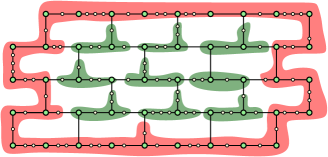
Figure 2: A $5$-wall and its canonical partition ${\cal Q}$. The red bag is the external bag $Q_{\rm ext}$.

For every $i,j\in[2,r-1]$, we denote by $Q^{(i,j)}$ the graph $A^{(i,j)}\cup B^{(i,j)}$ and by ${Q_{\rm ext}}$ the graph $W\setminus\bigcup_{i,j\in[2,r-1]}V(Q_{i,j})$. Now consider the collection ${\cal Q}=\{Q_{\rm ext}\}\cup\{Q_{i,j}\mid i,j\in[2,r-1]\}$ and observe that the graphs in ${\cal Q}$ are connected subgraphs of $W$ and their vertex sets form a partition of $V(W)$. We call ${\cal Q}$ the canonical partition of $W$. Also, we call every $Q_{i,j},i,j\in[2,r-1]$ an internal bag of ${\cal Q}$, while we refer to $Q_{\rm ext}$ as the external bag of ${\cal Q}$. See Figure 2 for an illustration of the notions defined above. For every $i\in[(r-1)/2]$, we say that a set $Q\in{\cal Q}$ is an $i$-internal bag of ${\cal Q}$ if $V(Q)$ does not contain any vertex of the first $i$ layers of $W$. Notice that the $1$-internal bags of ${\cal Q}$ are the internal bags of ${\cal Q}$.

Canonical partition of a graph with respect to a wall.

Let $W$ be a wall of a graph $G$. Consider the canonical partition ${\cal Q}$ of $W$. The enhancement of the canonical partition $\mathcal{Q}$ on $G$ is the following operation. We set $\tilde{\cal Q}:={\cal Q}$ and, as long as there is a vertex $x\in G\setminus V({\boldsymbol{\boldsymbol{\bigcup}}}\tilde{\cal Q})$ that is adjacent to a vertex of a graph $Q\in\tilde{\cal Q}$, we update $\tilde{\cal Q}:=\tilde{\cal Q}\setminus\{Q\}\cup\{\tilde{Q}\}$, where $\tilde{Q}=G[\{x\}\cup V(Q)]$. We call the $\tilde{Q}\in\tilde{\cal Q}$ that contains $Q_{\rm ext}$ as a subgraph the external bag of $\tilde{\cal Q}$, and we denote it by $\tilde{Q}_{\rm ext}$, while we call internal bags of $\tilde{\cal Q}$ all graphs in $\tilde{\cal Q}\setminus\{\tilde{Q}_{\rm ext}\}$. Moreover, we enhance $\tilde{\cal Q}$ by adding all vertices of $G\setminus\bigcup_{\tilde{Q}\in\tilde{\mathcal{Q}}}V(\tilde{Q})$ in its external bag, i.e., by updating $\tilde{Q}_{\rm ext}:=G[V(\tilde{Q}_{\rm ext})\cup V(G)\setminus\bigcup_{\tilde{Q}\in\tilde{\mathcal{Q}}}V(\tilde{Q})]$.

We call such a partition $\tilde{\cal Q}$ a $W$-canonical partition of $G$. Notice that a $W$-canonical partition of $G$ is not unique, since the sets in ${\cal Q}$ can be “expanded” arbitrarily when introducing vertex $x$.

Let $W$ be an $r$-wall of a graph $G$, for some odd integer $r\geq 3$ and let $\tilde{\cal Q}$ be a $W$-canonical partition of $G$. For every $i\in[(r-1)/2]$, we say that a set $Q\in\tilde{\cal Q}$ is an $i$-internal bag of $\tilde{\cal Q}$ if it contains an $i$-internal bag of ${\cal Q}$ as a subgraph.

We stress that given a graph $G$ and an $r$-wall $W$ of $G$ for some odd integer $r\geq 3$, a $W$-canonical partition $\tilde{\mathcal{Q}}$ of $G$ can have internal bags that are adjacent to vertices of arbitrarily many other bags. However, if $W$ is a flat wall of $G$ certified by some $7$-tuple $\mathfrak{R}$, the “flat structure” of the $\mathfrak{R}$-compass of $W$ implies that every bag can be adjacent to only bags that contain vertices of the same brick of $W$.

The next result is also proved in [SauST21kapiI] and intuitively states that, given a flatness pair $(W,\mathfrak{R})$ of “big enough” height and a $W$-canonical partition $\tilde{\mathcal{Q}}$ of $G$, we can find a “packing” of subwalls of $W$ that are inside some central part of $W$ and such that the vertex set of every internal bag of $\tilde{\cal Q}$ intersects the vertices of the flaps in the influence of at most one of these walls. We will use this result in the case where the set $A^{\prime}$ of Proposition 3.7 is “small”, i.e., there are only “few” vertices in $A$ that have “big enough” degree with respect to the central part of the canonical partition, and therefore Proposition 3.7 cannot justify branching. Following the latter condition and Proposition 5.4, we will be able to find a flatness pair with “few” apices so as to build irrelevant vertex arguments inside its compass. In [SauST21kapiI], $(W,\mathfrak{R})$-canonical partition is used to denote a $W$-canonical partition of $G$, where $(W,\mathfrak{R})$ is a flatness pair of $G$. However, in this subsection we provide a more general definition that does not take into account the flatness of $W$.

Proposition 5.4 (​​[SauST21kapiI]).

There exists a function $f_{13}:{\mathbb{N}}^{3}\to{\mathbb{N}}$ such that if $p,l\in{\mathbb{N}}_{\geq 1}$, $r\in{\mathbb{N}}_{\geq 3}$ is an odd integer, $G$ is a graph, $(W,\mathfrak{R})$ is a flatness pair of $G$ of height at least $\hyperref@@ii[@idealistic]{f_{\ref*{@idealistic}}}(l,r,p)$, and $\tilde{\mathcal{Q}}$ is a $W$-canonical partition of $G$, then there is a collection $\mathcal{W}=\{W^{1},\ldots,W^{l}\}$ of $r$-subwalls of $W$ such that

• for every $i\in[l]$, $\bigcup{\sf influence}_{\mathfrak{R}}(W^{i})$ is a subgraph of $\bigcup\{Q\mid Q\text{ is a $p$-internal bag of }\tilde{\mathcal{Q}}\}$ and

• for every $i,j\in[l]$, with $i\neq j$, there is no internal bag of $\tilde{\mathcal{Q}}$ that contains vertices of both $V(\bigcup{\sf influence}_{\mathfrak{R}}(W^{i}))$ and $V(\bigcup{\sf influence}_{\mathfrak{R}}(W^{j}))$.

Moreover, $\hyperref@@ii[@idealistic]{f_{\ref*{@idealistic}}}(l,r,p)=\mathcal{O}(\sqrt{l}\cdot r+p)$ and $\mathcal{W}$ can be constructed in time $\mathcal{O}(n+m)$.

5.5 Bidimensionality of sets

In this subsection, we present the notion of bidimensionality of a set with respect to a wall of a graph. This notion intuitively expresses the “spread” of a set $X$ in a $W$-canonical partition of $G$. The crucial idea is that a set $X$ of small bidimensionality cannot “destroy” a (flat) wall too much.

Bidimensionality.

Let $W$ be a wall of a graph $G$, $\tilde{\mathcal{Q}}$ be a $W$-canonical partition of $G$, and $X\subseteq V(G)$. The bidimensionality of $X$ in $G$ with respect to $\tilde{\mathcal{Q}}$, denoted by ${\sf bid}_{\tilde{\mathcal{Q}}}(X)$, is the number of internal bags of $\tilde{\mathcal{Q}}$ intersected by $X$. The bidimensionality of $X$ in $G$ with respect to $W$, denoted by ${\sf bid}_{G,W}(X)$, is the maximum bidimensionality of $X$ with respect to a $W$-canonical partition of $G$.

5.3 and Lemma 5.2 provide sets $X\subseteq V(G)$ that can be used to apply Proposition 3.7 to $\mathcal{F}$-M-Deletion and $\mathcal{F}$-M-Elimination Distance, respectively.

Every set $S\subseteq V(G)$ of size at most $k$ clearly has bidimensionality at most $k$.

Observation 5.3.

Let $\mathcal{F}$ be a finite collection of graphs, let $G$ be a graph, let $k\in{\mathbb{N}}$, and let $W$ be a wall of $G$. Then for every $k$-apex set $S$ of $G$ for ${\sf exc}(\mathcal{F})$ it holds that ${\sf bid}_{G,W}(S)\leq k$.

Moreover, given a $k$-elimination set $S$, we can find a set $X\supseteq S$ of bidimensionality at most $k(k+1)/2$ such that $G\setminus X\in{\sf exc}(\mathcal{F})$. To prove this, we first prove the following result, which intuitively states that a $k$-elimination set can intersect at most $k$ horizontal and vertical paths of a wall.

Lemma 5.1.

Let $\mathcal{F}$ be a finite collection of graphs. Let $G$ be a graph, let $k\in{\mathbb{N}}$, let $r,h$ be odd integers with $r\geq h+k$, let $W$ be an $r$-wall of $G$, and let $S$ be a $k$-elimination set of $G$ for ${\sf exc}(\mathcal{F})$. Then there is an $h$-subwall $W^{\prime}$ of $W$ with $V(W^{\prime})\cap S=\emptyset$.

Proof.

Since $S$ is a $k$-elimination set of $G$ for ${\sf exc}(\mathcal{F})$, there is an $\mathcal{F}$-elimination forest $(F,\chi,R)$ of $G$ of height $k$ such that $\chi({\sf Int}(F,R))=S$.

We set $W_{0}:=W$. For $i\in[k]$, we proceed to construct an $r_{i}$-subwall $W_{i}$ of the $r_{i-1}$-wall $W_{i-1}$ with $r_{i}\geq r-i$ such that for every $i\in[k]$ there is a node $z_{i}$ of $F$ such that $(F_{z_{i}},z_{i})$ has height at most $k-i$ and $V(W_{i})\subseteq\chi(V(F_{z_{i}}))$. This will imply the existence of a wall of size at least $r-k$ whose vertex set will be a subset of $\chi(V(F_{z})$, where $z\in{\sf Leaf}(F,R)$.

Let $S_{i}:=V(W_{i-1})\cap S$. If $S_{i}=\emptyset$, we set $W_{j}:=W_{i-1}$ for $j\in[i,k]$. Otherwise, let $u_{i}$ be the least common ancestor of $\chi^{-1}(S_{i})$ in $(F,R)$. According to Lemma 4.1, since $W_{i-1}$ is connected, $u_{i}$ exists and belongs to $\chi^{-1}(S_{i})$.

We obtain an $(r_{i-1}-1)$-subwall $W_{i}$ of $W_{i-1}$ that does not contain $\chi(u_{i})$ by taking the wall containing all horizontal and vertical paths of $W_{i-1}$ aside from the ones intersecting $u_{i}$ and we set $r_{i}:=r_{i-1}-1$ (to simplify the argument, here we call the resulting graph a wall even when the height is even). Note that since $W_{i}$ is a subgraph of $G[\chi(V(F_{u_{i}}))]$ that is connected, there is a $z_{i}\in{\sf Ch}_{F_{u_{i}},u_{i}}(u_{i})$ such that $V(W_{i})\subseteq V(F_{z_{i}})$. Notice that $(F_{u_{i}},\chi|_{V(F_{u_{i}}},u_{i})$ is an $\mathcal{F}$-elimination forest of $G[\chi(F_{u_{i}})]$ of height at most $k-i$.

Observe that $z_{k}$ should be a leaf of $(F,R)$ and therefore, since we have that $V(W_{k})\subseteq V(F_{z_{k}})\subseteq V(G)\setminus S$, $W_{k}$ is a wall of $G\setminus S$ of height at least $r-k\geq h$. ∎

Now we prove our result regarding the bidimensionality of $k$-elimination sets.

Lemma 5.2.

Let $\mathcal{F}$ be a finite collection of graphs. Let $G$ be a graph, let $A\subseteq V(G)$, let $k\in{\mathbb{N}}$, let $r\geq 2k+3$ be an odd integer, let $(W,\mathfrak{R})$ be a flatness pair of $G\setminus A$, and let $S$ be a $k$-elimination set of $G$ for ${\sf exc}(\mathcal{F})$. There is a set $X\supseteq S$ such that $G\setminus X\in{\sf exc}(\mathcal{F})$ and ${\sf bid}_{G\setminus A,W}(X)\leq k(k+1)/2$.

Proof.

Let $p={\sf odd}(r-k)$. Let $W^{\prime}$ be a $p$-subwall of $W$ that is a wall of $G\setminus S$, which exists due to Lemma 5.1. Let $C$ be the connected component of $G\setminus S$ that contains $W^{\prime}$. Since $C\in{\sf exc}(\mathcal{F})$, $K_{s_{\mathcal{F}}}$ is not a minor of $C$. Moreover, since $S$ is a $k$-elimination set of $G$ for ${\sf exc}(\mathcal{F})$, there is a set $P\subseteq S$ of size at most $k$ such that $(L,R):=(V(G)\setminus V(C),V(C)\cup P)$ is a separation of $G$ with $L\cap R=P$.

Let us show that ${\sf bid}_{G\setminus A,W}(V(G)\setminus V(C))\leq k(k+1)/2$. Let $\tilde{\mathcal{Q}}$ be a $W$-canonical partition of $G\setminus A$. Let $l$ be the number of internal bags of $\tilde{\mathcal{Q}}$ intersected by $P$ and note that $l\leq k$.

Let $G^{\prime}$ be the graph obtained from $G$ after contracting each bag of $\tilde{\mathcal{Q}}$ to a vertex. It is easy to observe that $G^{\prime}$ is isomorphic to a planar supergraph of an $h$-grid $H$, where $h=r-2$, together with an additional vertex that is adjacent to every vertex of the perimeter of $H$.

We let $[h]^{2}$ be the vertex set of $H$, where $(i,j)$ and $(i^{\prime},j^{\prime})$ are adjacent if and only if $|i-i^{\prime}|+|j-j^{\prime}|=1$. We will show that there is a separation $(L^{\prime},R^{\prime})$ of $H$ of order at most $l$ that maximizes $\min\{|L^{\prime}|,|R^{\prime}|\}$. Let $A=L^{\prime}\cap R^{\prime}$. We suppose without loss of generality that $|L^{\prime}|\leq|R^{\prime}|$. Notice that $l<h$. We take $A:=\{(i,j)\in[h]^{2}\mid i+j=l\}$, i.e., $L^{\prime}$ is the set of pairs of indices in the triangle bounded by $(0,0)$, $(0,l)$, and $(l,0)$. Thus, $|L^{\prime}|=l(l+1)/2$. It is easy to verify that this maximizes $|L^{\prime}|$.

Therefore, since the vertices of $H$ are the internal bags of $\tilde{\mathcal{Q}}$ and $P$ intersects $l$ internal bags, it implies that one of $L$ and $R$ intersects at most $l(l+1)/2\leq k(k+1)/2$ internal bags of $\tilde{\mathcal{Q}}$. Recall that $W^{\prime}$ is a wall of $C$ of height $p$. It is easy to verify that an elementary $x$-wall $W^{*}$ has $2x^{2}-2$ vertices with $8x-10$ vertices in the perimeter. Hence, it has $2(x-2)^{2}$ vertices not in the perimeter, and therefore the canonical partition of $W^{*}$ has $(x-2)^{2}$ internal bags. Thus, the canonical partition of $W^{\prime}$ has $(p-2)^{2}$ internal bags. Observe that each such a bag is contained in an internal bag of $\tilde{\mathcal{Q}}$ and therefore $V(C)$ intersects at least $(p-2)^{2}$ internal bags of $\tilde{\mathcal{Q}}$. Since $(p-2)^{2}\geq(r-k-2)^{2}\geq(k+1)^{2}>k(k+1)/2$, it holds that ${\sf bid}_{G\setminus A,W}(V(C)\cup P)>k(k+1)/2$. Therefore, ${\sf bid}_{G\setminus A,W}(V(G)\setminus V(C))\leq k(k+1)/2$. ∎

5.6 Homogeneous walls

In this subsection, we define homogeneous flat walls. Intuitively, homogeneous flat walls are flat walls that allow the routing of the same set of (topological) minors in the augmented flaps (i.e., the flaps together with the apex set) “cropped” by each one of their bricks. Such a flat wall can be detected in a big enough flat wall (Proposition 3.5) and this “homogeneity” property implies that some central part of a big enough homogeneous wall can be declared irrelevant (Proposition 3.6). The results presented in this subsection are from [SauST21kapiI, SauST21kapiII].

Folios.

We say that $(M,T)$ is a tm-pair if $M$ is a graph, $T\subseteq V(M)$, and all vertices in $V(M)\setminus T$ have degree two. We denote by ${\sf diss}(M,T)$ the graph obtained from $M$ by dissolving all vertices in $V(M)\setminus T$. A tm-pair of a graph $G$ is a tm-pair $(M,T)$ where $M$ is a subgraph of $G$. We call the vertices in $T$ branch vertices of $(M,T)$. We need to deal with topological minors for the notion of homogeneity defined below, on which the statement of [BasteST20acom, Theorem 5.2] relies. If $\textbf{M}=(M,B,\rho)\in{\cal B}$ and $T\subseteq V(M)$ with $B\subseteq T$, we call $(\textbf{M},T)$ a btm-pair and we define ${\sf diss}(\textbf{M},T)=({\sf diss}(M,T),B,\rho)$. Note that we do not permit dissolution of boundary vertices, as we consider all of them to be branch vertices. If $\textbf{G}=(G,B,\rho)$ is a boundaried graph and $(M,T)$ is a tm-pair of $G$ where $B\subseteq T$, then we say that $(\textbf{M},T)$, where $\textbf{M}=(M,B,\rho)$, is a btm-pair of $\textbf{G}=(G,B,\rho)$. Let $\textbf{G}_{1},{\bf G}_{2}$ be two boundaried graphs. We say that $\textbf{G}_{1}$ is a topological minor of $\textbf{G}_{2}$, denoted by $\textbf{G}_{1}{\preceq_{\sf tm}}\textbf{G}_{2}$, if $\textbf{G}_{2}$ has a btm-pair $(\textbf{M},T)$ such that ${\sf diss}(\textbf{M},T)$ is isomorphic to $\textbf{G}_{1}$. Given a $\textbf{G}\in{\cal B}$ and a positive integer $\ell$, we define the $\ell$-folio of ${\bf G}$ as

$${\ell}\mbox{\sf-folio}(\textbf{G})=\{\textbf{G}^{\prime}\in{\cal B}\mid\textbf{G}^{\prime}{\preceq_{\sf tm}}\textbf{G}\mbox{\leavevmode\nobreak\ and $\textbf{G}^{\prime}$ has detail at most $\ell$}\}.$$

Augmented flaps.

Let $G$ be a graph, $A$ be a subset of $V(G)$ of size $a$, and $(W,\mathfrak{R})$ be a flatness pair of $G\setminus A$. For each flap $F\in{\sf Flaps}_{\mathfrak{R}}(W)$ we consider a labeling $\ell_{F}:\partial F\rightarrow\{1,2,3\}$ such that the set of labels assigned by $\ell_{F}$ to $\partial F$ is one of $\{1\}$, $\{1,2\}$, $\{1,2,3\}$. Also, let $\tilde{a}\in[a]$. For every set $\tilde{A}\in\binom{A}{\tilde{a}}$, we consider a bijection $\rho_{\tilde{A}}:\tilde{A}\to[\tilde{a}]$. The labelings in ${\cal L}=\{\ell_{F}\mid F\in{\sf Flaps}_{\mathfrak{R}}(W)\}$ and the labelings in $\{\rho_{\tilde{A}}\mid\tilde{A}\in\binom{A}{\tilde{a}}\}$ will be useful for defining a set of boundaried graphs that we will call augmented flaps. We first need some more definitions.

Given a flap $F\in{\sf Flaps}_{\mathfrak{R}}(W)$, we define an ordering $\Omega(F)=(x_{1},\ldots,x_{q})$, with $q\leq 3$, of the vertices of $\partial{F}$ so that

• $(x_{1},\ldots,x_{q})$ is a counter-clockwise cyclic ordering of the vertices of $\partial F$ as they appear in the corresponding cell of $C(\Gamma)$. Notice that this cyclic ordering is significant only when $|\partial F|=3$, in the sense that $(x_{1},x_{2},x_{3})$ remains invariant under shifting, i.e., $(x_{1},x_{2},x_{3})$ is the same as $(x_{2},x_{3},x_{1})$ but not under inversion, i.e., $(x_{1},x_{2},x_{3})$ is not the same as $(x_{3},x_{2},x_{1})$, and

• for $i\in[q]$, $\ell_{F}(x_{i})=i$.

Notice that the second condition is necessary for completing the definition of the ordering $\Omega(F)$, and this is the reason why we set up the labelings in ${\cal L}$.

For each set $\tilde{A}\in\binom{A}{\tilde{a}}$ and each $F\in{\sf Flaps}_{\mathfrak{R}}(W)$ with $t_{F}:=|\partial F|$, we fix $\rho_{F}:\partial F\to[\tilde{a}+1,\tilde{a}+t_{F}]$ such that $(\rho^{-1}_{F}(\tilde{a}+1),\ldots,\rho^{-1}_{F}(\tilde{a}+t_{F}))=\Omega(F)$. Also, we define the boundaried graph

$$\textbf{F}^{\tilde{A}}:=(G[\tilde{A}\cup F],\tilde{A}\cup\partial F,\rho_{\tilde{A}}\cup\rho_{F})$$

and we denote by $F^{\tilde{A}}$ the underlying graph of $\textbf{F}^{\tilde{A}}$. We call $\textbf{F}^{\tilde{A}}$ an $\tilde{A}$-augmented flap of the flatness pair $(W,\mathfrak{R})$ of $G\setminus A$ in $G$.

Palettes and homogeneity.

For each $\mathfrak{R}$-normal cycle $C$ of ${\sf Compass}_{\mathfrak{R}}(W)$ and each set $\tilde{A}\subseteq A$, we define $(\tilde{A},\ell)\mbox{\sf-palette}(C)=\{\ell\mbox{\sf-folio}({\bf F}^{\tilde{A}})\mid F\in{\sf influence}_{\mathfrak{R}}(C)\}$. Given a set $\tilde{A}\subseteq A$, we say that the flatness pair $(W,\mathfrak{R})$ of $G\setminus A$ is $\ell$-homogeneous with respect to $\tilde{A}$ if every internal brick of ${W}$ has the same $(\tilde{A},\ell)$-palette (seen as a cycle of ${\sf Compass}_{\mathfrak{R}}(W)$). Also, given a collection ${\cal S}\subseteq 2^{A}$, we say that the flatness pair $(W,\mathfrak{R})$ of $G\setminus A$ is $\ell$-homogeneous with respect to ${\cal S}$ if it is $\ell$-homogeneous with respect to every $\tilde{A}\in{\cal S}$.

6 Vertex deletion to a minor-closed graph class

In this section, we prove our main result for the $\mathcal{F}$-M-Deletion problem. The following theorem is a restatement of Theorem 1.2 using the reformulation introduced in Subsection 2.2.

Theorem 6.1.

For every finite collection of graphs $\mathcal{F}$, there exists an algorithm that, given a graph $G$ and a non-negative integer $k$, runs in time $2^{k^{\mathcal{O}_{\ell_{\mathcal{F}}}(1)}}\cdot n^{2}$ and either outputs a $k$-apex set of $G$ for ${\sf exc}{(\mathcal{F})}$ or reports that such a set does not exist.

This algorithm is a generalization of the algorithm in the apex-minor free case of [SauST21kapiII]. In order to give an algorithm without the apex-minor restriction, we enhance the techniques of [SauST21kapiII] with some new tricks. We present this algorithm in this paper as a stepping stone to present the algorithms for elimination distance in LABEL:@oeconomicus and LABEL:@stubbornly, since the techniques used are similar (however not the same).

6.1 Description of the algorithm for $\mathcal{F}$-M-Deletion

Our algorithm for $\mathcal{F}$-M-Deletion has three steps. In Step 1, either we can easily conclude with a positive or a negative answer or we find a big wall. If we can find a large flat wall of bounded treewidth inside this wall, then we go to Step 2 and find an irrelevant vertex. Otherwise, we proceed to Step 3 where, by using flow techniques, we find a set of vertices that intersects every solution, and we branch on this set or we report a negative answer. The correctness of the algorithm is not trivial and will be justified in Subsection 6.2. While the general scheme of the algorithm is similar to the algorithm in [SauST21kapiII] for $\mathcal{F}$-M-Deletion in the case where $\mathcal{F}$ contains an apex-graph, here, in order to obtain a quadratic algorithm for general $\mathcal{F}$, we employ additional novel tricks so as to deal with the possible existence of many apices in all graphs in $\mathcal{F}$.

We define the following constants.

$$a= \ \hyperref@@ii[@collaboration]{f_{\ref*{@collaboration}}}(s_{\mathcal{F}}+a_{\mathcal{F}}-1), b= \ \hyperref@@ii[@collaboration]{f_{\ref*{@collaboration}}}(s_{\mathcal{F}}),$$

$$q= \ \hyperref@@ii[@categories]{f_{\ref*{@categories}}}(a_{\mathcal{F}},s_{\mathcal{F}},k), p= \ \hyperref@@ii[@provincial]{f_{\ref*{@provincial}}}(a_{\mathcal{F}},s_{\mathcal{F}},k),$$

$$l= \ (q-1)\cdot(k+b), r_{6}= \ \hyperref@@ii[@differences]{f_{\ref*{@differences}}}(a+b,\ell_{\mathcal{F}},3,k)$$

$$d= \ \hyperref@@ii[@deliberation]{f_{\ref*{@deliberation}}}(a+b,\ell_{\mathcal{F}}) r_{5}= \ \hyperref@@ii[@philistines]{f_{\ref*{@philistines}}}(r_{6},a+b,a+b,d),$$

$$t= \ \hyperref@@ii[@corollaries]{f_{\ref*{@corollaries}}}(s_{\mathcal{F}})\cdot r_{5}, r_{4}= \ {\sf odd}(t+3),$$

$$r_{3}= \ \hyperref@@ii[@idealistic]{f_{\ref*{@idealistic}}}(a_{\mathcal{F}},r_{4},1), r_{2}= \ {\sf odd}(2+\hyperref@@ii[@classifications]{f_{\ref*{@classifications}}}(s_{\mathcal{F}}+a_{\mathcal{F}}-1)\cdot r_{3}),$$

$$r_{2}^{\prime}= \ {\sf odd}(\max\{\hyperref@@ii[@unaffected]{f_{\ref*{@unaffected}}}(a_{\mathcal{F}},s_{\mathcal{F}},k),\hyperref@@ii[@idealistic]{f_{\ref*{@idealistic}}}(l+1,r_{2},p)\}), r_{1}= \ {\sf odd}(\hyperref@@ii[@classifications]{f_{\ref*{@classifications}}}(s_{\mathcal{F}})\cdot r_{2}^{\prime}+k).$$

Note that $r_{6}=\mathcal{O}_{\ell_{\mathcal{F}}}(k)$, $r_{5},r_{4},r_{3},r_{2},t=\mathcal{O}_{\ell_{\mathcal{F}}}(k^{c})$ and $r_{2}^{\prime},r_{1}=\mathcal{O}_{\ell_{\mathcal{F}}}(k^{c+2})$ where $c=\hyperref@@ii[@withdrawing]{f_{\ref*{@withdrawing}}}(a+b,a+b,d)$. Recall from Subsection 2.2 that we assume that $G$ has $\mathcal{O}_{s_{\mathcal{F}}}(k\sqrt{\log k}\cdot n)$ edges.

Step 1.

Run the algorithm Find-Wall from Proposition 3.1 with input $(G,r_{1},k)$ and, in time $2^{\mathcal{O}_{\ell_{\mathcal{F}}}(r_{1}^{2}+(k+r_{1})\log(k+r_{1}))}\cdot n=2^{\mathcal{O}_{\ell_{\mathcal{F}}}(k^{2(c+2)})}\cdot n$,

• either report a no-instance, or

• conclude that ${\sf tw}(G)\leq\hyperref@@ii[@veneration]{f_{\ref*{@veneration}}}(s_{\mathcal{F}})\cdot r_{1}+k$ and solve $\mathcal{F}$-M-Deletion in time $2^{\mathcal{O}_{\ell_{\mathcal{F}}}((r_{1}+k)\log(r_{1}+k))}\cdot n=2^{\mathcal{O}_{\ell_{\mathcal{F}}}(k^{c+2}\cdot\log k)}\cdot n$ using the algorithm of Proposition 3.2, or

• obtain an $r_{1}$-wall $W_{1}$ of $G$.

If the output of Proposition 3.1 is an $r_{1}$-wall $W_{1}$, consider all the $\binom{r_{1}}{r_{2}}^{2}=2^{\mathcal{O}_{\ell_{\mathcal{F}}}(k^{c}\log k)}$ $r_{2}$-subwalls of $W_{1}$. For each one of them, say $W_{2}$, let $W_{2}^{*}$ be the central $(r_{2}-2)$-subwall of $W_{2}$ and let $D_{W_{2}}$ be the graph obtained from $G$ after removing the perimeter of $W_{2}$ and taking the connected component containing $W_{2}^{*}$. Run the algorithm Grasped-or-Flat of Proposition 3.3 with input $(D_{W_{2}},r_{3},s_{\mathcal{F}}+a_{\mathcal{F}}-1,W_{2}^{*})$. This can be done in time $\mathcal{O}_{s_{\mathcal{F}}}(k\sqrt{\log k}\cdot n)$.

If for some of these subwalls the result is a set $A\subseteq V(D_{W_{2}})$ with $|A|\leq a$ and a flatness pair $(W_{3},\mathfrak{R}_{3})$ of $D_{W_{2}}\setminus A$ of height $r_{3}$ then, as in Proposition 5.4, compute a $W_{3}$-canonical partition $\tilde{\mathcal{Q}}$ of $D_{W_{2}}\setminus A$ and a collection $\mathcal{W}=\{W^{1},...,W^{a_{\mathcal{F}}}\}$ of $r_{4}$-subwalls of $W_{3}$ such that for every $i\in[a_{\mathcal{F}}]$, $\bigcup{\sf influence}_{\mathfrak{R}_{3}}(W^{i})$ is a subgraph of $\bigcup\{Q\mid Q\text{ is a $p$-internal bag of }\tilde{\mathcal{Q}}\}$ and for every $i,j\in[a_{\mathcal{F}}]$, with $i\neq j$, there is no internal bag of $\tilde{\mathcal{Q}}$ that contains vertices of both $V(\bigcup{\sf influence}_{\mathfrak{R}_{3}}(W^{i}))$ and $V(\bigcup{\sf influence}_{\mathfrak{R}_{3}}(W^{j}))$. This can be done in time $\mathcal{O}_{s_{\mathcal{F}}}(k\sqrt{\log k}\cdot n)$.

For $i\in[a_{\mathcal{F}}]$, let $W^{i*}$ be the central $(r_{4}-2)$-subwall of $W^{i}$ and let $D_{W^{i}}$ be the graph obtained from $D_{W_{2}}$ after removing $A$ and the perimeter of $W^{i}$ and taking the connected component containing $W^{i*}$. Run the algorithm Clique-or-twFlat of Proposition 3.4 with input $(D_{W^{i}},r_{5},s_{\mathcal{F}})$. This takes time $2^{\mathcal{O}_{\ell_{\mathcal{F}}}(r_{5}^{2})}\cdot n=2^{\mathcal{O}_{\ell_{\mathcal{F}}}(k^{2c})}\cdot n$. If for one of these subwalls the result is a set $A^{\prime}$ of size at most $b$ and a regular flatness pair $(W_{5},\mathfrak{R}_{5})$ of $D_{W^{i}}\setminus A^{\prime}$ of height $r_{5}$ whose $\mathfrak{R}_{5}$-compass has treewidth at most $t$, then we proceed to Step 2.

If, for every flatness pair $(W_{3},\mathfrak{R}_{3})$ and for every $i\in[a_{\mathcal{F}}]$, the result is a report that $K_{s_{\mathcal{F}}}$ is a minor of $D_{W^{i}}$, then we proceed to Step 3.

Step 2 (irrelevant vertex case).

We obtain a 7-tuple $\mathfrak{R}_{5}^{\prime}$ by adding all vertices of $G\setminus V({\sf Compass}_{\mathfrak{R}_{5}}(W_{5}))$ to the set in the first coordinate of $\mathfrak{R}_{5}$, such that $(W_{5},\mathfrak{R}_{5}^{\prime})$ is a regular flatness pair of $G\setminus(A\cup A^{\prime})$ whose $\mathfrak{R}_{5}^{\prime}$-compass has treewidth at most $t$. We apply the algorithm Homogeneous of Proposition 3.5 with input $(r_{6},a+b,a+b,d,t,G,A\cup A^{\prime},W_{5},\mathfrak{R}_{5}^{\prime})$, which outputs, in time $2^{\mathcal{O}_{\ell_{\mathcal{F}}}(t\log t+k\log k)}\cdot n=2^{\mathcal{O}_{\ell_{\mathcal{F}}}(k^{c}\log k)}\cdot n$, a flatness pair $(W_{6},\mathfrak{R}_{6})$ of $G\setminus(A\cup A^{\prime})$ of height $r_{6}$ that is $d$-homogeneous with respect to $2^{A\cup A^{\prime}}$ and is a $W^{*}$-tilt of $(W_{5},\mathfrak{R}_{5}^{\prime})$ for some subwall $W^{*}$ of $W_{5}$. We apply the algorithm Find-Irrelevant-Vertex of Proposition 3.6 with input $(k,a+b,G,A\cup A^{\prime},W_{6},\mathfrak{R}_{6})$, which outputs, in time $\mathcal{O}(n+m)=\mathcal{O}_{\ell_{\mathcal{F}}}(k\sqrt{\log k}\cdot n)$, a vertex $v$ such that $(G,k)$ and $(G\setminus v,k)$ are equivalent instances of $\mathcal{F}$-M-Deletion. Then the algorithm runs recursively on the equivalent instance $(G\setminus v,k)$.

Step 3 (branching case).

Consider all the $r_{2}^{\prime}$-subwalls of $W_{1}$, which are at most $\binom{r_{1}}{r_{2}^{\prime}}^{2}=2^{\mathcal{O}_{\ell_{\mathcal{F}}}(k^{c+2}\log k)}$ many, and for each of them, say $W_{2}^{\prime}$, compute its canonical partition $\mathcal{Q}$. Then, contract each bag $Q$ of $\mathcal{Q}$ to a single vertex $v_{Q}$, and add a new vertex $v_{\rm all}$ and make it adjacent to all $v_{Q}$’s. In the resulting graph $G^{\prime}$, for every vertex $y$ of $G\setminus V(W_{2}^{\prime})$, check, using a flow augmentation algorithm [Diestel10grap], whether there are $q$ internally vertex-disjoint paths from $v_{\rm all}$ to $y$ in time $\mathcal{O}(q\cdot m)=\mathcal{O}_{\ell_{\mathcal{F}}}(k^{4}\sqrt{\log k}\cdot n)$. Let $\tilde{A}$ be the set of all such $y$’s.

If $|\tilde{A}|<a_{\mathcal{F}}$, then report a no-instance.

If $a_{\mathcal{F}}\leq|\tilde{A}|\leq k+b$, then consider all the $\binom{|\tilde{A}|}{a_{\mathcal{F}}}=2^{\mathcal{O}_{\ell_{\mathcal{F}}}(\log k)}$ subsets of $\tilde{A}$ of size $a_{\mathcal{F}}$. For each one of them, say $A^{*}$, construct $\tilde{\mathcal{Q}}$ by enhancing $\mathcal{Q}$ on $G\setminus A^{*}$. Then, we distinguish two cases depending on whether for every $A^{*}$ all its vertices are adjacent to vertices of $q$ $p$-internal bags of $\tilde{\mathcal{Q}}$.

If each vertex of $A^{*}$ is adjacent to vertices of $q$ $p$-internal bags of $\tilde{\mathcal{Q}}$, then (due to Proposition 3.7) $A^{*}$ should intersect every solution of $\mathcal{F}$-M-Deletion for the instance $(G,k)$. Therefore, the algorithm runs recursively on each instance $(G\setminus y,k-1)$ for $y\in A^{*}$. If one of them is a yes-instance with $(k-1)$-apex set $S$ of $G\setminus y$, then $(G,k)$ is a yes-instance with $k$-apex set $S\cup\{y\}$ of $G$. If all of them are no-instances, then report a no-instance. This concludes the case where each vertex of $A^{*}$ is adjacent to vertices of $q$ $p$-internal bags of $\tilde{\mathcal{Q}}$.

If for every subset $A^{*}$ of $\tilde{A}$ of size $a_{\mathcal{F}}$, there is a vertex of $A^{*}$ that is not adjacent to vertices of $q$ $p$-internal bags of the given $\tilde{\mathcal{Q}}$, then report a no-instance. This concludes the case that $a_{\mathcal{F}}\leq|\tilde{A}|\leq k+b$.

If for every wall, $|\tilde{A}|>k+b$, then report that $(G,k)$ is a no-instance of $\mathcal{F}$-M-Deletion.

Notice that Step 3, when applied, takes time $2^{\mathcal{O}_{\ell_{\mathcal{F}}}(k^{c+2}\log k)}\cdot n^{2}$, because we apply the flow algorithms to each of the $2^{\mathcal{O}_{\ell_{\mathcal{F}}}(k^{c+2}\log k)}$ $r_{2}^{\prime}$-subwalls and for each vertex of $G$. However, the search tree created by the branching technique has at most $a_{\mathcal{F}}$ branches and depth at most $k$. So Step 3 cannot be applied more than ${a_{\mathcal{F}}}^{k}$ times during the course of the algorithm. Since Step 1 runs in time $2^{\mathcal{O}_{\ell_{\mathcal{F}}}(k^{2(c+2)})}\cdot n$, Step 2 runs in time $2^{\mathcal{O}_{\ell_{\mathcal{F}}}(k^{2c})}\cdot n$, and both may be applied at most $n$ times, the claimed time complexity follows: the algorithm runs in time $2^{\mathcal{O}_{\ell_{\mathcal{F}}}(k^{2(c+2)})}\cdot n^{2}$.

6.2 Correctness of the algorithm

Suppose first that $(G,k)$ is a yes-instance and let $S$ be a $k$-apex set of $G$. The application of the algorithm Find-Wall of Proposition 3.1 with input $(G,r_{1},k)$ either returns a report that ${\sf tw}(G)\leq\hyperref@@ii[@veneration]{f_{\ref*{@veneration}}}(s_{\mathcal{F}})\cdot r_{1}+k$ or returns an $r_{1}$-wall. In the first case, i.e., if ${\sf tw}(G)\leq\hyperref@@ii[@veneration]{f_{\ref*{@veneration}}}(s_{\mathcal{F}})\cdot r_{1}+k$, the application of the algorithm of Proposition 3.2 correctly outputs a $k$-apex set of $G$. We will focus on the latter case, i.e., where the algorithm Find-Wall returns an $r_{1}$-wall of $G$, say $W_{1}$. Since $r_{1}\geq\hyperref@@ii[@classifications]{f_{\ref*{@classifications}}}(s_{\mathcal{F}})\cdot r_{2}^{\prime}+k$, there is an $(\hyperref@@ii[@classifications]{f_{\ref*{@classifications}}}(s_{\mathcal{F}})\cdot r_{2}^{\prime})$-subwall of $W_{1}$, say $W_{1}^{*}$, that does not contain vertices of $S$. Since $G\setminus S$ does not contain $K_{s_{\mathcal{F}}}$ as a minor, there is no model of $K_{s_{\mathcal{F}}}$ grasped by $W_{1}^{*}$ and therefore, due to Proposition 3.3 with input $(G\setminus S,r_{2}^{\prime},s_{\mathcal{F}},W_{1}^{*})$, we know that there is a set $B\subseteq V(G\setminus S)$, with $|B|\leq b$, and a flatness pair $(W_{2}^{\prime},\mathfrak{R}_{2}^{\prime})$ of $G\setminus(S\cup B)$ of height $r_{2}^{\prime}$ such that $W_{2}^{\prime}$ is a $W^{\prime\prime}$-tilt of some subwall $W^{\prime\prime}$ of $W_{1}^{*}$.

Let $\mathcal{Q}$ be the canonical partition of $W_{2}^{\prime}$. Let $G^{\prime}$ be the graph obtained by contracting each bag $Q$ of $\mathcal{Q}$ to a single vertex $v_{Q}$, and adding a new vertex $v_{\rm all}$ and making it adjacent to all $v_{Q}$’s. Let $\tilde{A}$ be the set of vertices $y$ of $G\setminus V(W_{2}^{\prime})$ such that there are $q$ internally vertex-disjoint paths from $v_{\rm all}$ to $y$ in $G^{\prime}$. We claim that $\tilde{A}\subseteq S\cup B$. To show this, we first prove that, for every $y\notin S\cup B$, the maximum number of internally vertex-disjoint paths from $v_{\sf all}$ to $y$ in $G^{\prime}$ is $k+b+4$. Indeed, if $y$ is a vertex in the $\mathfrak{R}_{2}^{\prime}$-compass of $W_{2}^{\prime}$, there are at most $k+b$ such paths that intersect the set $S\cup B$ and at most four paths that do not intersect $S\cup B$ (in the graph $G^{\prime}\setminus(S\cup B)$) due to the fact that $(W_{2}^{\prime},\mathfrak{R}_{2}^{\prime})$ is a flatness pair of $G\setminus(S\cup B)$. If $y$ is not a vertex in the $\mathfrak{R}_{2}^{\prime}$-compass of $W_{2}^{\prime}$, then, since by the definition of flatness pairs the perimeter of $W_{2}^{\prime}$ together with the set $S\cup B$ separate $y$ from the $\mathfrak{R}_{2}^{\prime}$-compass of $W_{2}^{\prime}$, every collection of internally vertex-disjoint paths from $v_{\rm all}$ to $y$ in $G^{\prime}$ should intersect the set $\{v_{Q_{\rm ext}}\}\cup S\cup B$, where $Q_{\rm ext}$ is the external bag of $\mathcal{Q}$. Therefore, in both cases, if $y\notin S\cup B$, the maximum number of internally vertex-disjoint paths from $v_{\sf all}$ to $y$ in $G^{\prime}$ is $k+b+4$. Since $k+b+4<q$, we have that $y\notin\tilde{A}$. Hence, $\tilde{A}\subseteq S\cup B$ and therefore $|\tilde{A}|\leq k+b$. Hence, if $(G,k)$ is a yes-instance we cannot have that $|\tilde{A}|>k+b$, so the algorithm correctly reports a no-instance at the end of Step 3.

Let $\tilde{\mathcal{Q}}$ be a $W_{2}^{\prime}$-canonical partition of $G\setminus(S\cup B)$ obtained by enhancing $\mathcal{Q}$ on $G\setminus(S\cup B)$. Let $\tilde{A}^{\prime}$ be the set of vertices in $S\cup B$ that are adjacent to vertices of at least $q$ $p$-internal bags of $\tilde{\mathcal{Q}}$ (recall that $\tilde{A}$ is the set of vertices in $S\cup B$ that are adjacent to vertices of at least $q$ internal bags of $\tilde{\mathcal{Q}}$). Note that $\tilde{A}^{\prime}\subseteq\tilde{A}$ and therefore $|\tilde{A}^{\prime}|\leq|\tilde{A}|$.

If $|\tilde{A}^{\prime}|<a_{\mathcal{F}}$, then at most $a_{\mathcal{F}}-1$ vertices of $S\cup B$ are adjacent to vertices of at least $q$ $p$-internal bags of $\tilde{\mathcal{Q}}$. This means that the $p$-internal bags of $\tilde{\mathcal{Q}}$ that contain vertices adjacent to some vertex of $(S\cup B)\setminus\tilde{A}^{\prime}$ are at most $(q-1)\cdot(k+b)=l$.

Consider a family $\mathcal{W}=\{W^{1},\ldots,W^{l+1}\}$ of $l+1$ $r_{2}$-subwalls of $W_{2}^{\prime}$ such that for every $i\in[l+1]$, $\bigcup{\sf influence}_{\mathfrak{R}_{2}^{\prime}}(W^{i})$ is a subgraph of $\bigcup\{Q\mid Q\text{ is a $p$-internal bag of }\tilde{\mathcal{Q}}\}$ and for every $i,j\in[l+1]$, with $i\neq j$, there is no internal bag of $\tilde{\mathcal{Q}}$ that contains vertices of both $V(\bigcup{\sf influence}_{\mathfrak{R}_{2}^{\prime}}(W^{i}))$ and $V(\bigcup{\sf influence}_{\mathfrak{R}_{2}^{\prime}}(W^{j}))$. The existence of $\mathcal{W}$ follows from Proposition 5.4 and the fact that $r_{2}^{\prime}\geq\hyperref@@ii[@idealistic]{f_{\ref*{@idealistic}}}(l+1,r_{2},p)$.

The fact that the $p$-internal bags of $\tilde{\mathcal{Q}}$ that contain vertices adjacent to some vertex of $(S\cup B)\setminus\tilde{A}^{\prime}$ are at most $l$ implies that there exists an $i\in[l+1]$ such that no vertex of $V(\bigcup{\sf influence}_{\mathfrak{R}_{2}^{\prime}}({W^{i}}))$ is adjacent, in $G$, to a vertex in $(S\cup B)\setminus\tilde{A}^{\prime}$. Let $W_{2}:=W^{i}$, let $W_{2}^{*}$ be the central $(r_{2}-2)$-subwall of $W_{2}$, and let $D_{W_{2}}$ be the graph obtained from $G$ by removing the perimeter of $W_{2}$ and taking the connected component that contains $W_{2}^{*}$. Since no vertex of $V(\bigcup{\sf influence}_{\mathfrak{R}_{2}^{\prime}}({W^{i}}))$ is adjacent, in $G$, to a vertex in $(S\cup B)\setminus\tilde{A}^{\prime}$, any path in $D_{W_{2}}$ going from a vertex of $W_{2}^{*}$ to a vertex in $S$ must intersect a vertex of $\tilde{A}^{\prime}$. Thus, there is no model of $K_{s_{\mathcal{F}}+a_{\mathcal{F}}-1}$ grasped by $W_{2}^{*}$ in $D_{W_{2}}$, because otherwise, $K_{s_{\mathcal{F}}}$ would be a minor of $G\setminus S$. So, by applying the algorithm Grasped-or-Flat of Proposition 3.3 with input $(D_{W_{2}},r_{3},s_{\mathcal{F}}+a_{\mathcal{F}}-1,W_{2}^{*})$, since $r_{2}-2\geq\hyperref@@ii[@classifications]{f_{\ref*{@classifications}}}(s_{\mathcal{F}}+a_{\mathcal{F}}-1)\cdot r_{3}$, we should find a set $A\subseteq V(D_{W_{2}})$ with $|A|\leq a$ and a flatness pair $(W_{3},\mathfrak{R}_{3})$ of $D_{W_{2}}\setminus A$ of height $r_{3}$, such that $W_{3}$ is a tilt of some subwall $\tilde{W}_{3}$ of $W_{2}$.

Let $\tilde{\mathcal{Q}}^{\prime}$ be a $W_{3}$-canonical partition of $D_{W_{2}}\setminus A$. Let $\mathcal{W}^{\prime}=\{W^{1},...,W^{a_{\mathcal{F}}}\}$ be a collection of $r_{4}$-subwalls of $W_{3}$ such that for every $i\in[a_{\mathcal{F}}]$, $\bigcup{\sf influence}_{\mathfrak{R}_{3}}(W^{i})$ is a subgraph of $\bigcup\{Q\mid Q\text{ is an internal bag of }\tilde{\mathcal{Q}}^{\prime}\}$ and for every $i,j\in[a_{\mathcal{F}}]$, with $i\neq j$, there is no internal bag of $\tilde{\mathcal{Q}}^{\prime}$ that contains vertices of both $V(\bigcup{\sf influence}_{\mathfrak{R}_{3}}(W^{i}))$ and $V(\bigcup{\sf influence}_{\mathfrak{R}_{3}}(W^{j}))$. Since $|\tilde{A}^{\prime}|<a_{\mathcal{F}}$, there is an $i\in[a_{\mathcal{F}}]$ such that $V(\bigcup{\sf influence}_{\mathfrak{R}_{3}}(W^{i}))$ does not intersect $\tilde{A}^{\prime}$. The existence of $\mathcal{W}^{\prime}$ follows from Proposition 5.4 and the fact that $r{}_3\ge \text{<a href="\#S5.Thmproposition4" title="Proposition 5.4 ([SauST21kapiI]). ‣ Canonical partition of a graph with respect to a wall. ‣ 5.4 Canonical partitions ‣ 5 Even more definitions: Flat walls ‣ Efficient parameterized algorithms for modification problems to minor-closed classes" class="ltx\_ref"><span class="ltx\_text ltx\_ref\_tag">5.4</span></a>}$