Robust Bayesian Inference for Moving Horizon Estimation

Abstract

The accuracy of moving horizon estimation (MHE) suffers significantly in the presence of measurement outliers. Existing methods address this issue by treating measurements leading to large MHE cost function values as outliers, which are subsequently discarded. This strategy, achieved through solving combinatorial optimization problems, is confined to linear systems to guarantee computational tractability and stability. Contrasting these heuristic solutions, our work reexamines MHE from a Bayesian perspective, unveils the fundamental issue of its lack of robustness: MHE’s sensitivity to outliers results from its reliance on the Kullback-Leibler (KL) divergence, where both outliers and inliers are equally considered. To tackle this problem, we propose a robust Bayesian inference framework for MHE, integrating a robust divergence measure to reduce the impact of outliers. In particular, the proposed approach prioritizes the fitting of uncontaminated data and lowers the weight of contaminated ones, instead of directly discarding all potentially contaminated measurements, which may lead to undesirable removal of uncontaminated data. A tuning parameter is incorporated into the framework to adjust the robustness degree to outliers. Notably, the classical MHE can be interpreted as a special case of the proposed approach as the parameter converges to zero. In addition, our method involves only minor modification to the classical MHE stage cost, thus avoiding the high computational complexity associated with previous outlier-robust methods and inherently suitable for nonlinear systems. Most importantly, our method provides robustness and stability guarantees, which are often missing in other outlier-robust Bayes filters. The effectiveness of the proposed method is demonstrated on simulations subject to outliers following different distributions, as well as on physical experiment data.

, , , ,

1 Introduction

Accurate state estimation from noisy measurements, combined with the knowledge of system dynamics, is a crucial aspect of effective control systems. This problem has attracted significant attention across diverse domains, including vehicle control, aerospace navigation, and power grid management. Bayesian filtering offers a principled approach to solving state estimation problems by relying on Bayes’ formula to update the posterior distribution of the system’s state [47, 12]. Building upon the foundation of Bayesian filtering, moving horizon estimation (MHE) has emerged as a powerful technique for obtaining accurate estimates in nonlinear systems [39]. MHE is formulated as a receding horizon optimization problem, which takes into account a finite number of past measurements. This formulation enables MHE to handle diverse noise distributions and to account for constraints on states and noises. Indeed, MHE becomes the Kalman filter (KF) when constraints are absent and only the latest measurement is considered.

The accuracy of state estimation can be severely degraded when the assumed measurement generation mechanism deviates from the true mechanism. This misspecification of the measurement model, which may arise from sensor malfunction or inaccurate noise modeling, presents a significant challenge in maintaining estimation accuracy. Measurements affected by such misspecification, often referred to as outliers, necessitate careful handling to ensure the reliability of state estimates.

Outlier-robust MHE was first studied in [2, 3], where a mixed-integer optimization problem was formulated to tackle the issue of measurement outliers. At each time instant, a set of least-squares cost functions is minimized, with the potential outlier-affected measurements being left out in turn. Subsequently, based on the assumption that outliers lead to a large value of cost function, only the minimizer associated with the lowest cost is selected as the estimate. A significant issue with this method is that simply discarding contaminated measurements can potentially lead to the loss of valuable information. Moreover, this strategy assumes bounded values of the measurement noise and intermittent outliers, which can limit its applicability as real-world noise and outliers often exhibit unbounded behavior and unpredictable distributions. Furthermore, it is constrained to be applicable only to linear systems in order to ensure stability and computational tractability, given the complexity of solving NP-hard mixed-integer optimization problems [15, 2, 3].

To address the degradation of estimation accuracy caused by the presence of measurement outliers, robust Bayesian inference (RBI) provides a systematic solution [28, 29, 1]. It is revealed in RBI theory that the sensitivity of Bayesian inference to outliers arises from its equal consideration of outliers and inliers. This sensitivity is due to the inherent mechanism of Bayesian inference, which aims to minimize the Kullback-Leibler (KL) divergence between the assumed measurement likelihood and the true data-generating mechanism. This revelation motivates us to reinterpret MHE from a Bayesian perspective, differing from the optimization viewpoint in most MHE literature, enabling the application of RBI to mitigate the impact of outliers rather than merely discarding contaminated measurements. However, directly applying RBI to Bayesian filtering lacks robustness and stability guarantees [9], which are indispensable properties for state estimators. This theoretical gap highlights the necessity for a novel approach that can not only handle outliers effectively but also assure robustness and stability.

Capitalizing on the theory of RBI and recognizing the theoretical gap when applying it to MHE, this paper proposes an outlier-robust MHE framework that maintains robustness and preserves stability in the presence of measurement outliers. We rectify the sensitivity issue of KL divergence by introducing the $\beta$-divergence to assign lower weight to outliers, thereby mitigating their impact. Furthermore, we present a thorough analysis of robustness and stability when applying RBI to MHE, compared to our prior work [10]. Specifically, the key contributions of this paper can be summarized as follows:

1. We propose the $\beta$-MHE algorithm, which incorporates $\beta$-divergence into MHE for improved state estimation in the presence of outliers. This approach includes a tunable parameter, which allows for the adjustment of robustness degree against outliers. Notably, standard MHE is a special case of $\beta$-MHE when the parameter approaches zero. Further, the proposed algorithm necessitates only a minor modification to the MHE stage cost, circumventing the need for linearity assumptions and avoiding the NP-hardness issues associated with mixed-integer optimization in current robust MHE methods [2, 3].

2. We analytically derive the influence functions for MHE methods, providing a solid foundation for analyzing their robustness. Significantly, for linear Gaussian systems, we prove that the influence function of the proposed $\beta$-MHE is bounded, which demonstrates its robustness. This is the first work that systematically investigates the robustness of MHE from the perspective of influence function.

3. We analyze the stability of $\beta$-MHE by leveraging state-of-the-art stability results in MHE. We establish that, for a system exhibiting input/output-to-state stability and a cost function bounded by $\mathcal{K}$ functions with contraction properties, the proposed method ensures robustly asymptotically stable when the horizon length is sufficiently large.

The remainder of this paper unfolds as follows: Section 2 surveys the relevant literature. The problem formulation and preliminaries are presented in Section 3. Our proposed algorithm for outlier-robust MHE is introduced in Section 4. Section 5 and Section 6 study robustness and stability of $\beta$-MHE respectively. Simulation results are demonstrated in Section 7, while experimental results are provided in Section 8. Finally, we wrap up with conclusions in Section 9.

Notation: $\mathcal{D}_{\text{KL}}(\cdot||\cdot)$ and $\mathcal{D}_{\beta}(\cdot||\cdot)$ are the Kullback–Leibler divergence and the $\beta$-divergence of two probability distributions, respectively. $\delta(\cdot,\cdot)$ represents the Dirac function. The set of real numbers is denoted as $\mathbb{R}$, and the set of nonnegative real numbers is denoted as $\mathbb{R}_{+}$. The set of integers that lie in the interval $[a,b]$ is denoted by $\mathbb{Z}_{[a,b]}$. A function $\alpha:\mathbb{R}_{+}\to\mathbb{R}_{+}$ is a $\mathcal{K}$ function if it is continuous, strictly monotone increasing and $\alpha(0)=0$. A function $\alpha:\mathbb{R}_{+}\to\mathbb{R}_{+}$ is a $\mathcal{L}$ function if it is continuous, nonincreasing, and $\alpha\to 0$ if $t\to\infty$. A function $\alpha:\mathbb{R}_{+}\times\mathbb{R}_{+}\to\mathbb{R}_{+}$ is a $\mathcal{KL}$ function if for $\forall t$, $\alpha(\cdot,t)$ is a $\mathcal{K}$ function and $\forall s$, $\alpha(s,\cdot)$ is a $L$ function. $M\succeq 0$ indicates that the matrix $M$ is positive semi-definite, while $M\succ 0$ indicates that the matrix $M$ is positive-definite. $\|x\|$ represents the $l_{2}$-norm of the vector $x$, i,e., $\|x\|=\sqrt{x^{\top}x}$. We denote $\|x\|_{a:b}:=\max_{t\in\mathbb{Z}_{[a,b]}}\left\{\|x_{t}\|\right\}$ and $\|x\|_{0:\infty}:=\sup_{t\in\mathbb{Z}_{[0,\infty]}}\left\{\|x_{t}\|\right\}$. For $M\succeq 0$, $\|x\|_{M}$ is short for $\sqrt{x^{\top}Mx}$. $\|M\|_{\mathcal{F}}$ is the Frobenius norm of matrix $M$ while $|M|$ signifies the determinant of the matrix $M$. Besides, $\mathbb{I}_{n\times n}$ is the identity matrix with dimension $n$.

2 Related Works

In this section, we first introduce existing Bayesian filtering techniques besides MHE, which typically ignore the presence of outliers. Subsequently, we examine how these traditional techniques have been modified to tackle the outlier problem. Finally, we broaden our scope to $H_{\infty}$ filtering, a robust state estimation method for outlier mitigation that operates outside the Bayesian filtering framework.

2.1 Bayesian filtering

Under the assumptions of linearity and Gaussianity, Bayesian filtering can simplify to the well-known KF, which acquires state estimates recursively and analytically [27]. However, a closed-form estimator like KF does not exist for nonlinear systems, as nonlinear functions cannot maintain the property of Gaussian. To circumvent this limitation, several KF variants have been proposed, such as the extended KF (EKF) and the unscented KF (UKF) [26, 41]. Nevertheless, these methods still suffer from reduced estimation accuracy, particularly in highly nonlinear systems or under low signal-to-noise ratios. In contrast, particle filter (PF) uses sequential Monte Carlo method to approximate the posterior distribution with a finite number of samples. While PF theoretically converges to the true distribution as the number of samples approaches infinity, its extensive computational requirements limit its practical use [12]. A significant weakness shared by all these methods is their sensitivity to measurement outliers. Such outliers can significantly impair estimation accuracy, emphasizing the need for robust estimation techniques.

2.2 Outlier-robust Bayesian filtering

To address the significant challenge of measurement outliers, various methods have been developed. For linear systems where KF is prevalent, numerous outlier-robust KF variants have emerged. For example, leveraging Schweppe’s proposal and the Huber function, a batch-mode maximum likelihood-type KF is proposed in [17]. Alternatively, the maximum correntropy KF substitutes the minimum mean square error criterion with the more robust maximum correntropy criterion [11]. Furthermore, a novel outlier-robust KF framework using a statistical similarity measure has been developed recently, illustrating that existing methods can be recovered or approximated by choosing different similarity functions [24].

While these methods can address the challenge of outliers in linear systems, capitalizing on the inherent structure of KF, they do not constitute a comprehensive, principled approach within the broader Bayesian framework. When these methods are extended to nonlinear systems, they often translate directly into outlier-robust EKF and UKF using linearization or unscented transformation techniques [35, 51, 52]. However, this direct translation lacks a solid theoretical foundation. In contrast, outlier-robust PFs have been developed independently, without relying on the recursive form of KF. They utilize techniques such as kernel density estimation [33], auxiliary particle filtering schemes [36], and hypothesis testing [37] to bolster their robustness against outliers. Regrettably, these methods for nonlinear systems lack robustness guarantees and stability analyses compared to the robust filters designed for linear systems, such as in [17, 2, 3]. This gap underlines the need for designing an outlier-robust filter for nonlinear systems with robustness and stability guarantees.

2.3 $H_{\infty}$ filtering

In our discussion of robust filtering approaches, the $H_{\infty}$ filter merits attention due to its unique objectives and robustness characteristics. Unlike the Kalman filter, which aims to minimize the mean-square error, the $H_{\infty}$ filter is designed to constrain the worst-case variance in state estimates, ensuring the minimization of estimation energy error for all fixed-energy disturbances [45]. Extensions for nonlinear systems such as the $H_{\infty}$ EKF, $H_{\infty}$ EKF and $H_{\infty}$ PF [13, 34, 50] have been developed, addressing nonlinear dynamics while maintaining robustness. However, the $H_{\infty}$ filtering approach is inherently conservative due to its design philosophy, which emphasizes worst-case scenarios. This results in a strategy that does not fully capitalize on available system model information, consequently leading to suboptimal performance.

3 Problem Formulation and Preliminaries

In this section, we present the problem formulation of MHE, comparing the conventional optimization-based viewpoint and a Bayesian perspective. We also introduce the state-space model formulation of MHE, laying the groundwork for a deeper exploration of its stability. Concluding this section, we revisit the optimization-centric interpretation of Bayesian inference, which forms the foundation for implementing RBI techniques.

3.1 Problem Formulation in a Bayesian View

MHE can be interpreted from two distinct viewpoints. Traditional research considers MHE as an optimization method, where a trajectory of state estimates is optimized online to fit the measurements with minimal noise estimates. In contrast, our perspective considers MHE as a tool for obtaining the maximum a posteriori (MAP) estimate within the framework of Bayesian inference.

Consider the stochastic systems characterized by the hidden Markov model (HMM):

$$x_{0} \sim\pi_{0}(x_{0}),$$ (1)

$$x_{t}|x_{t-1} \sim f(x_{t}|x_{t-1}),$$

$$y_{t}|x_{t} \sim g(y_{t}|x_{t}),$$

where $x_{t}$ represents the unobserved states of a Markov process and $y_{t}$ denotes the associated noisy measurements. Besides, $\pi_{0}$ represents the initial distribution of the state, $f$ is the transition probability, and $g$ is the likelihood function, also known as the emission probability. In this context, optimal state estimation aims to infer the true state $x_{t}$ of stochastic systems based on current and past measurements $y_{1:t}$. To this effect, Bayesian filtering is utilized to compute either the posterior marginal distribution $q_{t}(x_{t}|y_{1:t})$ or the posterior joint distribution $q_{t}(x_{0:t}|y_{1:t})$ that is factorized as

$$q_{t}(x_{0:t}|y_{1:t})=\pi_{0}(x_{0})\prod\limits_{i=1}^{t}g(y_{i}|x_{i})f(x_{i}|x_{i-1}).$$ (2)

For nonlinear systems with non-Gaussian noises, computing the posterior distributions becomes a challenging task. It is often more feasible to obtain a point estimate of the state instead of computing the entire density. For nonlinear systems, it is common to choose the MAP estimate due to the asymmetric and potentially multi-modal nature of the posterior distribution [40]. In light of this, full information estimation (FIE) targets the mode of the posterior joint distribution:

$$\hat{x}_{0|t},\hat{x}_{1|t},...,\hat{x}_{t|t}=\arg\max_{x_{0:t}}q_{t}(x_{0:t}|y_{1:t}).$$ (3)

However, the computational complexity of solving FIE in (3) rises with the number of available measurements. To maintain computational feasibility, MHE employs a sliding window approach, using a finite number of past measurements to simplify the problem. By leveraging logarithmic transformations, the MHE problem can be formulated as

$$\hat{x}_{t-T|t},\hat{x}_{t-T+1|t},...,\hat{x}_{t|t}=\arg\min_{x_{t-T:t}}J(x_{t-T:t}),$$ (4a)

$$J(x_{t-T:t})=\Gamma(x_{t-T})+\sum\limits_{i=t-T+1}^{t}\left\{k(x_{i},x_{i-1})+h(y_{i},x_{i})\right\},$$ (4b)

where

$$\Gamma(x_{t-T}) \approx-\log{q_{t-T}(x_{t-T}|y_{1:t-T})},$$ (5a)

$$k(x_{i},x_{i-1}) =-\log{f(x_{i}|x_{i-1})},$$ (5b)

$$h(y_{i},x_{i}) =-\log{g(y_{i}|x_{i})}.$$ (5c)

In this formulation, $\Gamma(x_{t-T})$ is referred to as the arrival cost (also known as the initial penalty), and $\mathbb{C}(x_{t},x_{t-1},y_{t})=k(x_{t},x_{t-1})+h(y_{t},x_{t})$ represents the stage cost function. For simplicity, we use $\hat{x}_{t-T:t}$ to represent $\left\{\hat{x}_{t-T|t},\hat{x}_{t-T+1|t},...,\hat{x}_{t|t}\right\}$.

Assumption 1.

We assume that the optimization problem defined by (4a)(4b) is well-posed, i.e., the solution of (4a)(4b) exists for $\forall t\in\mathbb{Z}_{[0,\infty)}$.

Remark 1.

The arrival cost is a fundamental concept in MHE, serving as an equivalent statistic for summarizing past measurements $y_{1:t-T}$. Typically, when approximating the posterior distribution $q_{t-T}(x_{t-T}|y_{1:t-T})$ with a Gaussian distribution, the arrival cost is chosen to be of the quadratic form $\|x_{t-T}-\hat{x}_{t-T|t-T}\|^{2}_{P^{-1}_{t-T}}$. Here, $\hat{x}_{t-T|t-T}$ denotes the optimal estimate calculated in the previous time $t-T$, and $P_{t-T}$ is the error covariance matrix, which can be determined using EKF [39] or UKF [38] through Ricatti equation.

In practical scenarios, the assumption that measurements are strictly generated by the likelihood function $g$ often fails, leading to outliers that can critically undermine MHE’s accuracy [2, 3]. Responding to this challenge, our work focuses on formulating an approach that can effectively handle these outliers within the MHE framework. Unlike previous outlier-robust MHE approaches that are constrained to linear systems and specific noise assumptions [2, 3], our work takes into account more general nonlinear systems, eliminating the need for stringent noise assumptions. Furthermore, in contrast to other outlier-robust Bayesian filtering techniques [35, 51, 52, 33, 36, 37] that lack robustness or stability guarantees, our methodology aims to provide these assurances, thereby improving the reliability of the estimator.

3.2 State Space Model Formulation of MHE

While the HMM-based formulation of MHE provides a clear probabilistic interpretation, the state space model (SSM) formulation proves more convenient for stability analysis. SSM can be expressed as:

$$x_{t+1} =\mathcal{F}(x_{t},\xi_{t}),$$

$$y_{t} =\mathcal{G}(x_{t})+\zeta_{t}.$$

Where $\mathcal{F}$ and $\mathcal{G}$ represent the transition and measurement functions, respectively, while $\xi_{t}$ and $\zeta_{t}$ denote the process and measurement noise. The transition function $\mathcal{F}$ in SSM aligns with the transition probability $f$ in HMM, with the measurement function $\mathcal{G}$ aligning with the likelihood function $g$. For example, if the measurement noise adheres to a normal distribution, i.e., $\zeta_{t}\sim\mathcal{N}(0,R)$, we can express the likelihood function as $g(y_{t}|x_{t})=\frac{1}{\sqrt{(2\pi)^{n_{\zeta}}|R|}}\exp\left(-\frac{1}{2}(y_{t}-\mathcal{G}(x_{t}))^{\top}R^{-1}(y_{t}-\mathcal{G}(x_{t})\right)$, where $n_{\zeta}$ is the dimension of $\zeta_{t}$.

For stability analysis, we can rewrite the stage cost $\mathbb{C}(x_{t},x_{t-1},y_{t})$ as $\mathbb{C}(\xi_{t-1},\zeta_{t})=k(\xi_{t-1})+h(\zeta_{t})$ and the objective function $J(x_{0:t})$ as $J(x_{0},\xi_{0:t-1})$ within the SSM framework. This transformation modifies the optimization variables to $\xi_{t-1}$ and $\zeta_{t}$. For instance, with $\zeta_{t}\sim\mathcal{N}(0,R)$, we can represent $h(y_{t},x_{t})$ as $h(\zeta_{t})=\frac{1}{2}\zeta_{t}^{\top}R^{-1}\zeta_{t}$, significantly streamlining the notation.

Remark 2.

In our study, we primarily focus on state estimation. Therefore, any control inputs that are known beforehand are treated as fixed constants. This treatment simplifies the ensuing optimization and associated analyses without sacrificing any critical information. For the sake of clarity and conciseness, these control inputs are omitted from the problem formulation.

3.3 An Optimization-centric View on Bayesian Inference

In this subsection, we review the optimization-centric perspective of Bayesian inference, laying the foundation of RBI and paving the way for our proposed approach. Bayesian inference calculates the posterior distribution $p_{\text{pos}}(x|y)$ utilizing a prior probability $\pi(x)$ and a likelihood function $g(y|x)$,

$$p_{\text{pos}}(x|y)=\frac{\pi(x)g(y|x)}{p(y)},\;p(y)=\int_{x}{\pi(x)g(y|x)\mathrm{d}x}.$$

From an optimization-centric perspective on Bayesian inference [28], the posterior distribution can be formulated as a solution to the optimization problem:

$$p_{\text{pos}}=\min_{\nu}\left\{\int{-\log{g(y|x)}\nu(x)\mathrm{d}x}+\mathcal{D}_{\text{KL}}(\nu||\pi)\right\},$$ (6)

$$\mathcal{D}_{\text{KL}}(\nu||\pi):=\int\nu(x)\log\left(\frac{\nu(x)}{\pi(x)}\right)\,\mathrm{d}x.$$

Indeed, the negative logarithm of the likelihood in (6), i.e., $-\log{g(y|x)}$, can be extended to a generalized loss function $\ell(x,y)$. This function captures the discrepancy between observed data and the assumed likelihood, resulting in a generalized optimization problem:

$$q=\min_{\nu}\left\{\int{\ell(x,y)\nu(x)\mathrm{d}x}+\mathcal{D}_{\text{KL}}(\nu||\pi)\right\}.$$ (7)

The resulting belief distribution $q$, also referred to as the Gibbs posterior [46], leads to a Bayes-type updating rule given by

$$q(x)=\pi(x)\frac{G(y|x)}{Z},\;Z=\int_{x}{\pi(x)G(y|x)\mathrm{d}x},$$

where $G(y|x):=\exp{\left(-\ell(x,y)\right)}$ denotes a generalized likelihood function. By strategically designing the loss function $\ell$, it is possible to achieve RBI, effectively mitigating the impact of outliers in the data.

Remark 3.

The optimization target of (6) is essentially the negative of the evidence lower bound (ELBO) used in variational inference. In detail, variational inference aims to maximize the ELBO [8], and our methodology seeks to minimize its negative counterpart.

4 Algorithm Design for Outlier-Robust MHE

In Section 3, we showed that the negative logarithm of the likelihood in Bayesian inference could be extended to a generalized likelihood function $G(y|x)=\exp{\left(-\ell(x,y)\right)}$. This insight also inspires a generalization of Bayesian filtering. Specifically, if we define the sequence of generalized likelihoods as $G(y_{t}|x_{t})=\exp{\left(-\ell(x_{t},y_{t})\right)}$, the joint generalized posterior distribution $q^{\prime}_{t}(x_{0:t}|y_{1:t})$ can be expressed as the product of $G(y_{t}|x_{t})$ and $f(x_{t}|x_{t-1})$, i.e.,

$$q^{\prime}_{t}(x_{0:t}|y_{1:t})=\pi_{0}(x_{0})\prod\limits_{i=1}^{t}G(y_{i}|x_{i})f(x_{i}|x_{i-1}).$$ (8)

Observe that when the loss function $\ell(x_{t},y_{t})$ is chosen to be the negative logarithm of the likelihood, i.e., $\ell(x_{t},y_{t})=-\log{g(y_{t}|x_{t})}$, (8) becomes the posterior distribution in Bayesian filtering (2). Under this circumstance, $G(y_{t}|x_{t})=\exp{\left(\log{g(y_{t}|x_{t})}\right)}=g(y_{t}|x_{t})$.

Essentially, maximizing $-\log{g(y_{t}|x_{t})}$ is equivalent to minimizing $\mathcal{D}_{\text{KL}}(p_{\text{true}}^{t}(y_{t})||g(y_{t}|x_{t}))$ [20, 16], which is the KL divergence between the true data-generating model, denoted as $p_{\text{true}}^{t}(y_{t})$, and the assumed likelihood function $g(y_{t}|x_{t})$. The sensitivity of KL divergence to outliers leads to the sensitivity of Bayesian filtering, as it treats all data points equally, without distinguishing between inliers and outliers [1]. To enhance the robustness of Bayesian filtering, a more robust divergence such as the $\beta$-divergence can be employed [20, 16].

Fig. 1 compares KL divergence and $\beta$-divergence for parameter estimation of a single Gaussian distribution. When optimizing KL divergence, both inliers and outliers are treated equally, leading to an estimate that can be significantly disturbed by outliers. Conversely, the optimization of $\beta$-divergence yields a more robust estimate. It de-emphasizes the impact of outliers and focuses on fitting the primary distribution [16]. This property makes $\beta$-divergence a suitable choice when dealing with measurement outliers.

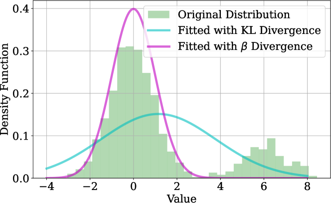
Figure 1: Comparison of the robustness of $\beta$-divergence and KL divergence for handling outliers. Here, the Gaussian distribution $\mathcal{N}(0,\;1)$ is contaminated with Gaussian distribution $\mathcal{N}(5,\;1)$ with probability 0.1.

The $\beta$-divergence between the true data distribution $p_{\text{true}}^{t}(\cdot)$ and the assumed likelihood $g(\cdot|x_{t})$ is given by

$$\mathcal{D}_{\beta}\left(p_{\text{true}}^{t}(\cdot)||g(\cdot|x_{t})\right)=\frac{1}{\beta}\int{p_{\text{true}}^{t}(y)^{\beta+1}\mathrm{d}y}$$ (9)

$$-\frac{\beta+1}{\beta}\int{p_{\text{true}}^{t}(y)g(y|x_{t})^{\beta}\mathrm{d}y}+\int{g(y|x_{t})^{\beta+1}\mathrm{d}y}.$$

Here, $\beta\in(0,1)$, and

$$\lim_{\beta\to 0}\mathcal{D}_{\beta}(\cdot||\cdot)=\mathcal{D}_{\text{KL}}(\cdot||\cdot).$$

The term $\frac{1}{\beta}\int{p_{\text{true}}^{t}(y)^{\beta+1}\mathrm{d}y}$ in (9) can be neglected because it is a constant value independent of $x_{t}$. Thus, the minimizer of $\mathcal{D}_{\beta}\left(p_{\text{true}}^{t}(\cdot)||g(\cdot|x_{t})\right)$ equals

$$\arg\min_{x_{t}}\Big{\{}-\frac{\beta+1}{\beta}\int{p_{\text{true}}^{t}(y)g(y|x_{t})^{\beta}\mathrm{d}y}$$ (10)

$$+\int{g(y|x_{t})^{\beta+1}\mathrm{d}y}\Big{\}}.$$

When applying the $\beta$-divergence in practice, since we cannot directly access the true data distribution $p_{\text{true}}^{t}(y)$ in (10), we use the empirical data distribution $p_{\text{em}}^{t}(y)=\delta(y-y_{t})$ as replacement [1, 9, 16, 20]. As a result, we can obtain the loss function $\ell^{\beta}(x_{t},y_{t})$ related to the $\beta$-divergence by substituting $p_{\text{true}}^{t}(y)$ with $p_{\text{em}}^{t}(y)$:

$$\ell^{\beta}(x_{t},y_{t})=-\frac{\beta+1}{\beta}g(y_{t}|x_{t})^{\beta}+\int{g(y|x_{t})^{\beta+1}\mathrm{d}y}.$$ (11)

When choosing $G(y_{t}|x_{t})$ as the “$\beta$ likelihood”

$$G^{\beta}(y_{t}|x_{t}):=\exp{\left(-\ell^{\beta}(x_{t},y_{t})\right)},$$ (12)

we can modify (5c) in the MHE objective to

$$h(y_{k},x_{k})=\ell^{\beta}(x_{k},y_{k}),$$ (13)

leading to the $\beta$-MHE algorithm. Note that the other components of the MHE algorithm are retained. Thus, the computational complexity of $\beta$-MHE aligns with that of MHE, since the only alteration lies in the (5c) and (13).

As summarized in Algorithm 1, the $\beta$-MHE algorithm achieves robustness to outliers by employing a cost function that leverages $\beta$-divergence. The choice of the parameter $\beta$ balances the robustness and accuracy of $\beta$-MHE, with smaller $\beta$ appropriate for minor measurement outliers, and larger $\beta$ suitable for significant measurement outliers. Notably, as $\beta$ approaches zero, $\beta$-MHE converges to the standard MHE, facilitating a smooth transition between the two methods.

Algorithm 1 $\beta$-MHE Algorithm

1:The hidden Markov model {$\pi_{0}$, $f$, $g$}, the estimation horizon $T$, the previous state estimate $\hat{x}_{t-T|t-T}$ at time $t-T$, and the measurements $y_{t-T+1:t}$

2:State estimate $\hat{x}_{t}$

3:if $0<t<T$ then

4:     The estimation horizon is reduced to $T^{\prime}=t$. Solve (4a),(4b),(5a),(5b),(13) using the arrival cost:

$$\Gamma(x_{0})=\|x_{0}-\hat{x}_{0|0}\|^{2}_{P^{-1}_{0}},$$

where $\hat{x}_{0}$ and $P_{0}$ are the mean and variance of the distribution $\pi_{0}$.

5:else

6:     Solve (4a),(4b),(5a),(5b),(13) using the arrival cost:

$$\Gamma(x_{t-T})=\|x_{t-T}-\hat{x}_{t-T|t-T}\|^{2}_{P^{-1}_{t-T}},$$

where $P_{t-T}$ is calculated via EKF or UKF.

5 Robustness Analysis

Robustness plays a pivotal role in characterizing the estimator’s ability to maintain accuracy in the presence of outliers[22, 21, 42, 25]. To evaluate the robustness of MHE, we utilize the influence function, a widely used measure in robust statistics determining an estimator’s sensitivity to outliers [22, 21, 25]. In particular, under linear Gaussian scenarios, we evaluate the supremum of the influence function for both MHE and $\beta$-MHE. Our findings confirm that the $\beta$-MHE, exhibiting a finite influence function, indeed provides improved robustness compared to MHE, which exhibits an unbounded influence function.

5.1 Influence Function of the MHEs

The influence function has been successfully implemented in robustness analyses of KFs [17, 32]. However, its application to the robustness analysis of MHE remains unexplored. This is mainly because previous works formulate MHE from an optimization standpoint, neglecting its essential nature as an inference problem. Existing robustness analyses for MHE are based on manually-designed robustness metrics [2, 3]. Unlike the influence function, these metrics lack a solid statistical foundation. Such manually-designed metrics restricts robustness analyses to linear systems, neglects process noise, and considers only bounded outliers [2, 3]. Recognizing this research gap, this subsection proposes the adoption of the influence function as a tool to facilitate the robustness analysis of nonlinear MHE.

As discussed in section 3, through an optimization-centric view on Bayesian inference, the loss function $\ell(x,y)$ in (7) is designed by minimizing the divergence between the empirical data distribution $p_{\text{em}}(y^{\prime})=\delta(y^{\prime}-y)$ and the likelihood function $g(y^{\prime}|x)$. Suppose the empirical data distribution is contaminated by a data point $z$ with probability $\epsilon$, such that $p_{\text{em}}(y^{\prime})=(1-\epsilon)\delta(y^{\prime}-y)+\epsilon\delta(y^{\prime}-z)$, the resulting estimator is then denoted as $\hat{x}\left((1-\epsilon)g+\epsilon\delta(z)\right)$ or simply as $\hat{x}^{z,\epsilon}$. Influence function is defined as the value of the derivative of $\hat{x}\left((1-\epsilon)g+\epsilon\delta(z)\right)$ with respect to the contamination probability $\epsilon$ at $\epsilon=0$:

$$\left.\mathbb{IF}(z,\hat{x},g)=\frac{\partial{}}{\partial{\epsilon}}\left[\hat{x}\left((1-\epsilon)g+\epsilon\delta(z)\right)\right]\right|_{\epsilon=0}.$$

Before we present our main result, we make the following assumption:

Assumption 2.

$J(x_{t-T:t})$ is twice continuously differentiable with respect to $x_{t-T:t}$ and its second derivative at the local minimum is nonsingular.

Remark 4.

Assumption 2 allows the derivation of an analytical form of the influence function. Assumption 2 is not overly restrictive, as it only necessitates a nonsingular Hessian matrix at the local minimum point. Besides, the twice continuous differentiability condition is naturally fulfilled in the case of MHE and $\beta$-MHE for linear Gaussian systems, which can be validated through the formulation of stage costs in (16) and (17).

The analytical expression of the influence function is presented in Theorem 1.

Theorem 1.

Under Assumption 1 and 2, the influence function of $\beta$-MHE for a general system (1) can be written as

$$\mathbb{IF}(z,\hat{x}_{t-T:t},G^{\beta}(y_{t}|x_{t}))=M_{1}^{-1}(\hat{x}_{t-T:t})\cdot M_{2}(z,\hat{x}_{t-T:t}),$$ (14a)

$$M_{1}(\hat{x}_{t-T:t}):=\left.\frac{\partial^{2}{\left[J(x_{t-T:t})\right]}}{\partial{x_{t-T:t}^{2}}}\right|_{x_{t-T:t}=\hat{x}_{t-T:t}},$$ (14b)

$$M_{2}(z,\hat{x}_{t-T:t}):=\sum\limits_{i=t-T+1}^{t}\left.\frac{\partial{\left[\mathscr{K}^{\beta,z}(x_{i},y_{i})\right]}}{\partial{x_{t-T:t}}}\right|_{x_{t-T:t}=\hat{x}_{t-T:t}},$$ (14c)

where $J(x_{t-T:t})$ is defined by (4b)(5a)(5b)(13) and $\mathscr{K}^{\beta,z}(x_{t},y_{t})=\frac{\beta+1}{\beta}{g(y_{t}|x_{t})^{\beta}}-\frac{\beta+1}{\beta}{g(z|x_{t})}^{\beta}$.

The proof of Theorem 1 can be found in Appendix A.

Corollary 1.

Similar results hold for the MHE when $\mathscr{K}^{\beta,z}(x_{t},y_{t})$ is restricted to $\mathscr{K}^{z}(x_{t},y_{t})=\log{g(y_{t}|x_{t})}-\log{g(z|x_{t})}$ and $J(x_{t-T:t})$ is defined by (4b)(5a)(5b)(5c).

Proof.

Let $\beta\to 0$, then the $\beta$-MHE converges to MHE, and therefore the results can be obtained for MHE. ∎

5.2 Gross Error Sensitivity of MHEs for Linear Guassian Systems

The previous subsection derives the influence function of $\beta$-MHE and MHE under a specific point of contamination. To comprehensively assess the estimator’s robustness, this subsection focuses on worst-case scenarios, namely considering the supremum of the influence function across all possible contamination points. This leads to the concept of gross error sensitivity [31].

Gross error sensitivity measures the maximum change a small perturbation to the likelihood $g$ at a point $z$ can induce to the estimate $\hat{x}$. It is defined as

$${\gamma}(\hat{x},g)=\sup_{z}\|\mathbb{IF}(z,\hat{x},g)\|.$$

We consider the typical linear Gaussian systems

$$x_{t+1}=Ax_{t}+\xi_{t},\quad y_{t}=Cx_{t}+\zeta_{t},$$ (15)

$$\xi_{t}\sim\mathcal{N}(0,\;Q),\quad\zeta_{t}\sim\mathcal{N}(0,\;R),\quad x_{0}\sim\mathcal{N}(0,\;P_{0}),$$

where $x_{t}\in\mathbb{R}^{n}$, $y_{t}\in\mathbb{R}^{m}$, $Q\succ 0$ and $R\succ 0$. The terms $\xi_{t}$ and $\zeta_{t}$ refer to the additive process noise and measurement noise, respectively. The arrival cost and the stage cost functions of MHE for system (15) are defined as

$$\Gamma(x_{t-T}) =\frac{1}{2}\|x_{t-T}-\hat{x}_{t-T|t-T}\|^{2}_{P_{t-T}^{-1}},$$ (16)

$$k(x_{t},x_{t-1}) =\frac{1}{2}\|x_{t}-Ax_{t-1}\|^{2}_{{Q}^{-1}},$$

$$h(y_{t},x_{t}) =\frac{1}{2}\|y_{t}-Cx_{t}\|^{2}_{{R}^{-1}}.$$

Here, $\hat{x}_{t-T|t-T}$ represents the optimal estimate from the previous time and $P_{t-T}$ refers to the error covariance matrix, which can be calculated recursively by solving the matrix Riccati equation [39]

$$P_{i+1}=Q+AP_{i}A^{\top}-AP_{i}C^{\top}(R+CP_{i}C^{\top})^{-1}CP_{i}A^{\top}.$$

The problem setting for the $\beta$-MHE method is largely similar to that of MHE, with the only adjustment being the modification of $h(y_{t},x_{t})$ in (16). Specifically, by substituting (5c) with (13), $h(y_{t},x_{t})$ in (16) is altered to

$$h(y_{t},x_{t}) =-\frac{\beta+1}{\beta\sqrt{(2\pi)^{\beta m}|R|^{\beta}}}e^{-\frac{\beta}{2}\|y_{t}-Cx_{t}\|^{2}_{{R}^{-1}}}$$ (17)

$$+\frac{1}{(\beta+1)^{\frac{1}{2}}(2\pi)^{\frac{m\beta}{2}}|R|^{\frac{\beta}{2}}}.$$

The subsequent theorem characterizes the robustness properties of MHE methods for linear Gaussian systems.

Theorem 2.

Under Assumption 1 and 2, the gross error sensitivity of MHE for system (15) is infinite while for that of $\beta$-MHE, it is bounded. Specifically, we have

$$\gamma(\hat{x}_{t-T:t},G^{\beta}(y_{t}|x_{t})) \leq 2\sqrt{T}\cdot\|M_{1}^{-1}(\hat{x}_{t-T:t})\|_{\mathcal{F}}\cdot\rho_{\text{max}},$$ (18)

where $M_{1}(\hat{x}_{t-T:t})$ is defined as (14b), and

$$\rho_{\text{max}} :=\max_{i\in\mathbb{Z}_{[t-T,t]}}\sup_{z}\|\rho(\hat{x}_{i},z)\|,$$ (19)

$$\rho(\hat{x}_{t},z) :=\frac{(\beta+1)C^{\top}R^{-1}}{\sqrt{(2\pi)^{\beta m}|R|^{\beta}}}(z-C\hat{x}_{t})e^{-\frac{\beta}{2}\|z-C\hat{x}_{t}\|^{2}_{{R}^{-1}}}.$$

The proof of Theorem 2 can be found in Appendix B.

Remark 5.

Due to the selected arrival cost, choosing the MHE horizon length $T=1$ recovers KF. Therefore, Theorem 2 also suits the robustness analysis of KF.

Theorem 2 provides an important conclusion: for linear Gaussian systems, the supremum of the influence function is finite for $\beta$-MHE, marking a distinct contrast to MHE, for which the supremum is infinite. This underscores the superior robustness offered by $\beta$-MHE over MHE.

6 Stability Analysis

The stability of MHE plays a significant role in its theoretical foundation, as it guarantees the estimates’ convergence to the true state [39, 23, 44, 5, 30, 7]. This section analyzes the stability of $\beta$-MHE inspired by the result in [4]. As a preliminary step, we introduce the concept of incremental input/output-to-state stability (i-IOSS) based on (20), which will play a key role in our subsequent analysis.

Definition 1 (i-IOSS).

The system $x_{t+1}=\mathcal{F}(x_{t},\xi_{t})$, $y_{t}=\mathcal{G}(x_{t})+\zeta_{t}$ is i-IOSS if there exist $\mathcal{KL}$ function $\gamma_{x}(\cdot,\cdot)$, and $\mathcal{K}$ functions $\gamma_{\xi}(\cdot),\gamma_{\zeta}(\cdot)$ which satisfy

$$\left\|x_{t}^{(1)}-x_{t}^{(2)}\right\| \leq\gamma_{x}\left(\left\|x_{0}^{(1)}-x_{0}^{(2)}\right\|,t\right)$$ (20)

$$\oplus\gamma_{\xi}\left(\left\|\xi^{(1)}-\xi^{(2)}\right\|_{0:t-1}\right)$$

$$\oplus\gamma_{\zeta}\left(\left\|y^{(1)}-y^{(2)}\right\|_{1:t}\right),\;\forall t\in\mathbb{Z}_{[0,\infty)}.$$

Here, $x_{t}^{(1)}$ and $x_{t}^{(2)}$ are two state sequences with initial states $x_{0}^{(1)}$ and $x_{0}^{(2)}$ respectively.

The concept of i-IOSS allows us to measure a system’s resistance to external perturbations. As summarised in Assumption 3, we assume the underlying system to be IOSS and the $\mathcal{KL}$ function $\gamma_{x}$ eventually become a contraction map on all intervals from the origin to $\bar{s}$.

Assumption 3.

The system $x_{t+1}=\mathcal{F}(x_{t},\xi_{t})$, $y_{t}=\mathcal{G}(x_{t})+\zeta_{t}$ is i-IOSS and furthermore, for every $\bar{s}>0$ and for every $\eta\in(0,1)$, there exists some $T_{m}\geq 0$ such that

$$\gamma_{x}(s,T_{m})\leq\eta s,$$ (21)

$\forall$ $s\leq\bar{s}$.

To further study the system’s stability properties, we proceed to introduce the definition of robustly asymptotically stable (RAS).

Definition 2 (RAS [4]).

An estimator is RAS if there exist $\bar{s},\delta>0$, $\mathcal{KL}$ functions $\rho_{x}(\cdot,\cdot)$, and $\mathcal{K}$ functions $\rho_{\xi}(\cdot),\rho_{\zeta}(\cdot)$ such that if $\|x_{0}-\hat{x}_{0|0}\|\leq\bar{s}$, $\|\xi\|_{0:\infty},\|\zeta\|_{0:\infty}\leq\delta$, then for $\forall t\in\mathbb{Z}_{[0,\infty)}$, we have

$$\left\|x_{t}-\hat{x}_{t|t}\right\| \leq\rho_{x}\left(\left\|x_{0}-\hat{x}_{0|0}\right\|,t\right)$$

$$\oplus\rho_{\xi}\left(\left\|\xi\right\|_{0:t-1}\right)$$

$$\oplus\rho_{\zeta}\left(\left\|\zeta\right\|_{1:t}\right).$$

To establish the RAS of MHE, we lay down two crucial assumptions.

Assumption 4.

The stage costs $k(\xi_{t})$ and $h(\zeta_{t})$ are bounded by $\mathcal{K}$ functions, i.e.,

$$\underline{\gamma}_{\xi}{(\|\xi_{t}\|)} \leq k(\xi_{t})\leq\bar{\gamma}_{\xi}{(\|\xi_{t}\|)},$$ (22)

$$\underline{\gamma}_{\zeta}{(\|\zeta_{t}\|)} \leq h(\zeta_{t})\leq\bar{\gamma}_{\zeta}{(\|\zeta_{t}\|)}.$$

Here, $\underline{\gamma}_{\xi},\bar{\gamma}_{\xi},\underline{\gamma}_{\zeta},\bar{\gamma}_{\zeta}$ are $\mathcal{K}$ functions.

Assumption 5.

For every $\bar{s}>0$ and $\eta\in(0,1)$, there exists $\mu>0$ such that $\gamma_{\xi}\left(2\underline{\gamma}_{\xi}^{-1}\Big{(}3\mu\cdot s^{2}\Big{)}\right)\leq\eta s$, $\gamma_{\zeta}\left(2\underline{\gamma}_{\zeta}^{-1}\Big{(}3\mu\cdot s^{2}\Big{)}\right)\leq\eta s$, $\forall$ $s\leq\bar{s}$.

Remark 6.

Assumption 4 assumes that the cost functions are bounded by $\mathcal{K}$ functions. This is a natural assumption that can be easily verified in most scenarios. For example, for the system with Gaussian noises, the stage costs $k(\xi_{t})=\frac{1}{2}\|\xi_{t}\|^{2}_{Q^{-1}}$ and $h(\zeta_{t})=\ell^{\beta}(\zeta_{t})=-\frac{\beta+1}{\beta\sqrt{(2\pi)^{\beta m}|R|^{\beta}}}e^{-\frac{\beta}{2}\|\zeta_{t}\|^{2}_{{R}^{-1}}}$ can be verified to satisfy (22) by noticing:

$$\frac{1}{2}\underline{\lambda}_{Q}\|\xi_{t}\|^{2} \leq\frac{1}{2}\|\xi_{t}\|^{2}_{Q^{-1}}\leq\frac{1}{2}\bar{\lambda}_{Q}\|\xi_{t}\|^{2},$$

$$-e^{-\frac{\beta}{2}\underline{\lambda}_{R}\|\zeta_{t}\|^{2}} \leq-e^{-\frac{\beta}{2}\|\zeta_{t}\|^{2}_{R^{-1}}}\leq-e^{-\frac{\beta}{2}\bar{\lambda}_{R}\|\zeta_{t}\|^{2}},$$

where $\underline{\lambda}_{Q},\bar{\lambda}_{Q}>0$ are the minimum and maximum eigenvalues of the matrix $Q^{-1}$, and $\underline{\lambda}_{R},\bar{\lambda}_{R}>0$ are the minimum and maximum eigenvalues of the matrix $R^{-1}$.

Following these assumptions, the stability of the corresponding $\beta$-MHE can be established:

Theorem 3.

Under Assumption 3, 4 and 5, for every $\bar{s}>0$, there exists a $T_{m}$ and $\bar{s}$ such that if $T\geq T_{m}$ and $\|\hat{x}_{0|0}-x_{0}\|\leq\bar{s}$, then there exist $\mathcal{KL}$ function $\rho_{x}$, $\mathcal{K}$ function $\rho_{\xi}$ and $\rho_{\zeta}$, and $\delta>0$, such that if $\|\xi\|_{0:\infty},\|\zeta\|_{0:\infty}\leq\delta$, then

$$\|x_{t}-\hat{x}_{t|t}\|\leq\rho_{x}(\|x_{0}-\hat{x}_{0|0}\|,t)\oplus\rho_{\xi}(\|\xi\|_{0:t-1})\oplus\rho_{\zeta}(\|\zeta\|_{1:t})$$ (23)

for $\forall t\in\mathbb{Z}_{[0,\infty)}$.

Theorem 3 builds RAS of $\beta$-MHE and its proof can be found in Appendix C.

In this section, we establish a sufficient condition for the stability of $\beta$-MHE. We find that to ensure stability in $\beta$-MHE, the system needs to exhibit IOSS properties, the cost function should be bounded by $\mathcal{K}$ functions with contraction properties, and the estimation length has to be sufficiently large. The stability analysis guarantees the convergence of the estimation error when performing the $\beta$-MHE algorithm.

7 Simulations

In this section, our aim is to assess the robustness of the $\beta$-MHE algorithm in the presence of outliers, as well as to investigate the effect of the $\beta$ parameter on this robustness. To this effect, we carry out two numerical simulations that showcase the performance of the algorithm. Throughout these simulations, we use the root mean squared error (RMSE) as an indicator of estimation accuracy. The RMSE measures the differences between the state estimation $\hat{x}_{t}$ and the actual state $x_{t}$:

$$\text{RMSE}=\sqrt{\frac{\sum_{t=1}^{N_{\text{step}}}\|x_{t}-\hat{x}_{t}\|^{2}}{n\cdot N_{\text{step}}}}.$$

In this equation, $N_{\text{step}}$ refers to the duration of the trajectory, and $n$ is the dimension of the state. The simulations are conducted on a laptop equipped with an AMD Ryzen 7 processor and 16.0 GB RAM. The optimization problems are handled using CasADi [6], an open-source solver for the efficient execution of nonlinear optimization tasks.

7.1 Linear System Case: Wiener Velocity Model

To initially test the robustness of our $\beta$-MHE algorithm in a linear system, we opt to use the Wiener velocity model, a commonly referenced model in filtering literatures [43, 49, 24]. Adopting a discretization step of $\Delta t=0.1$, we obtain a linear Gaussian stochastic model represented by (15). The state is expressed as $x=\left[\begin{matrix}p_{x}&p_{y}&\dot{p}_{x}&\dot{p}_{y}\end{matrix}\right]^{\top}$, encompassing the position coordinates $p_{x}$, $p_{y}$ and the velocities $\dot{p}_{x}$, $\dot{p}_{y}$. The parameters defined in (15) are shown as

$$A =\begin{bmatrix}1&0&\Delta t&0\\ 0&1&0&\Delta t\\ 0&0&1&0\\ 0&0&0&1\end{bmatrix},\;C=\begin{bmatrix}1&0&0&0\\ 0&1&0&0\end{bmatrix},$$

$$Q =\begin{bmatrix}\frac{\Delta t^{3}}{3}&0&\frac{\Delta t^{2}}{2}&0\\ 0&\frac{\Delta t^{3}}{3}&0&\frac{\Delta t^{2}}{2}\\ \frac{\Delta t^{2}}{2}&0&\Delta t&0\\ 0&\frac{\Delta t^{2}}{2}&0&\Delta t\end{bmatrix},\;R=\mathbb{I}_{2\times 2}.$$

To emulate the real-world scenario where measurements can be contaminated, we introduce noise following $\mathcal{N}(0,100^{2}\cdot\mathbb{I}_{2\times 2})$ with a probability $p_{c}$. To validate the robustness and performance of our proposed $\beta$-MHE algorithm, we compare it with MHE and KF across a varied range of $\beta$ values. The RMSE is evaluated over 100 Monte Carlo trials each consisting of 200 steps, i.e., $N_{\text{step}}=200$.

Fig. 2 displays the box plot of RMSE for different methodologies at $p_{c}=0.2$. Interestingly, we observe that the average RMSE demonstrates a decreasing trend as $\beta$ increases, until it attains its minimum at $\beta=10^{-4}$. This $\beta$ value emerged as a threshold from extensive experiments aiming to strike a balance between accuracy and robustness. Beyond this point, the RMSE begins to climb. Remarkably, when $\beta\leq 10^{-4}$, our proposed $\beta$-MHE achieves higher estimation accuracy compared to both the KF and the conventional MHE.

For further clarity, Fig. 3 presents the estimation error of the four states for different methods, where $\beta$ is set as $10^{-4}$. From a computational perspective, the average processing time per step for the KF, MHE, and $\beta$-MHE were recorded as 0.00023 ms, 0.024 ms, and 0.028 ms respectively. This indicates that the computational demand of our proposed $\beta$-MHE is comparable to that of the MHE.

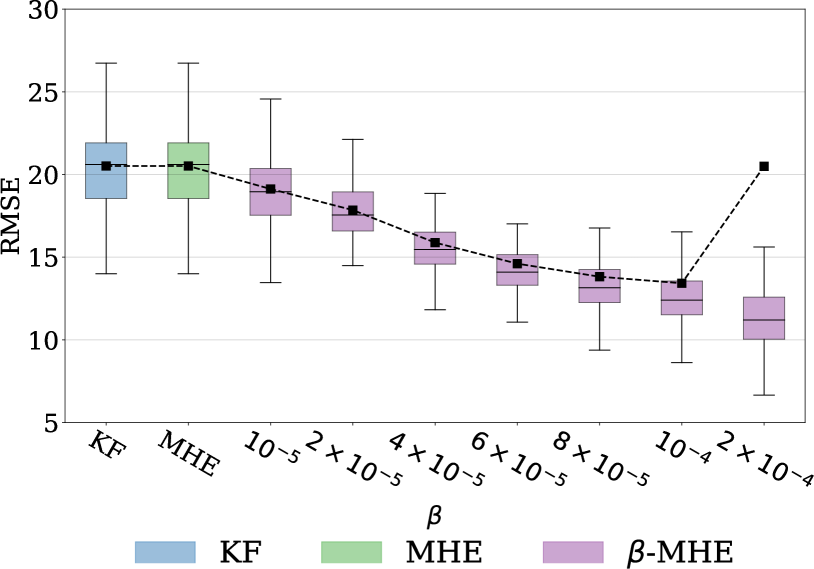
Figure 2: Box plot of RMSE for KF, MHE and $\beta$-MHE with different values of $\beta$ when contamination probability $p_{c}=0.2$. The black square “ $\blacksquare$ ” represents the average RMSE.

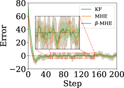
(a)

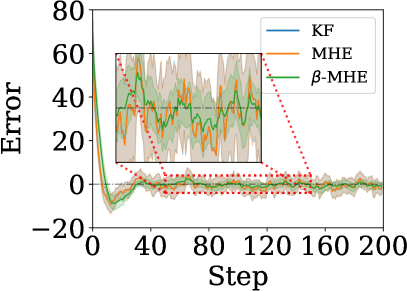
(b)

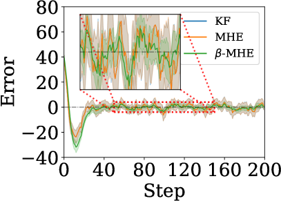
(c)

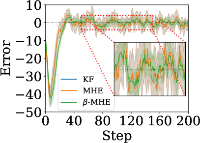
(d)

Figure 3: (a) Estimation error of $p_{x}$. (b) Estimation error of $p_{y}$. (c) Estimation error of $\dot{p}_{x}$. (d) Estimation error of $\dot{p}_{y}$. The solid lines correspond to the mean and the shaded regions correspond to $95\%$ confidence interval over 100 runs. Given that the MHE horizon length T is chosen as 1, the result of MHE, illustrated as the blue line, is identical to that of the KF, depicted by the orange line.

7.2 Nonlinear System Case: Isothermal Gas-phase Reactor Model

In this subsection, we perform simulation on an isothermal gas-phase reactor model, a model commonly referenced in MHE literature [48, 19, 18, 44]. This model describes the reversible reaction $2A_{r}\rightleftharpoons B_{r}$. Initially, the reactor is charged with certain amounts of $A_{r}$ and $B_{r}$, but the exact composition of the original mixture remains uncertain. The state $x$ includes the partial pressures, i.e., $x=\left[\begin{matrix}P_{A}&P_{B}\end{matrix}\right]^{\top}$. The discrete-time version of the gas-phase reactor model with the one-step Euler method ($\Delta t=0.1$) is

$${P}_{A,t+1} ={P}_{A,t}+\left(-2k_{1}P_{A,t}^{2}+2k_{2}P_{B,t}\right)\cdot\Delta t+\xi_{1,t},$$

$${P}_{B,t+1} ={P}_{B,t}+\left(k_{1}{P}_{A,t}^{2}-k_{2}{P}_{B,t}\right)\cdot\Delta t+\xi_{2,t},$$

where $k_{1}=0.16$, $k_{2}=0.0064$, $\xi_{t}\sim\mathcal{N}(0,\;10^{-4}\mathbb{I}_{2\times 2})$, and $x_{0}\sim\mathcal{N}(0,\;\mathbb{I}_{2\times 2})$. A pressure gauge measures the total pressure of the system as the species react, i.e.,

$$y_{t}=P_{A,t}+P_{B,t}+\zeta_{t},$$

where $\zeta_{t}\sim\mathcal{N}(0,\;0.01)$. It is proved in [44] that this system has IOSS property. We simulate measurement outliers as the impulsive noise drawing from a Student’s t distribution with $\nu=1$ degrees of freedom. Strictly speaking, we define $\zeta_{t}\sim p_{c}\cdot t_{\nu=1}(0,\;0.01)+(1-p_{c})\cdot\mathcal{N}(0,\;0.01)$. We evaluate the results for our proposed $\beta$-MHE, the MHE, and UKF for different contamination probabilities. As shown in Fig. 4, our method surpasses UKF and the MHE under different contamination probabilities and remains effective when there are no outliers. Besides, the estimation error of the two states is illustrated in Fig. 5, where $\beta$ is chosen as $10^{-4}$ and $p_{c}=0.2$. It is noticeable that the estimation error of UKF and MHE varies considerably, whereas for $\beta$-MHE, it remains relatively stable. Besides, the average computation time of each step for UKF, the MHE, and the $\beta$-MHE are 0.015 ms, 0.451 ms, and 0.495 ms respectively, which reveals the computational burdens of the proposed $\beta$-MHE and the MHE are at the same level for nonlinear systems.

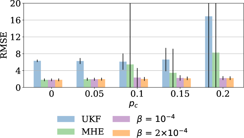
Figure 4: Bar plot of RMSE for UKF, MHE, and $\beta$-MHE with different contamination probabilities. The height of each bar represents the average RMSE value for a particular method under a specific contamination level. The error bars extending from the top of each bar indicate the standard deviation of the RMSE values over 100 runs, representing the variability in performance for each method. In addition, the MHE horizon length $T$ equals 3.

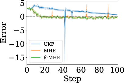
(a)

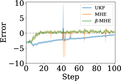
(b)

Figure 5: (a) Estimation error of $P_{A}$. (b) Estimation error of $P_{B}$. The solid lines correspond to the mean, and the shaded regions correspond to $95\%$ confidence interval over 100 runs.

8 Experiment: Warehouse Vehicle Localization

In this section, we carry out a real-world experiment involving indoor vehicle localization to assess the robustness and accuracy of our proposed algorithm. The experiment is conducted on a warehouse vehicle outfitted with a Lidar sensor, which supplies the necessary measurement data for real-time estimation of the vehicle’s position and heading angle.

8.1 Experimental Setup

In this experiment, we utilized a differential-drive vehicle equipped with a Lidar sensor for environment perception, as depicted in Fig. 6. The vehicle state is represented by $x=\left[\begin{matrix}p_{x}&p_{y}&\theta\end{matrix}\right]^{\top}$, including its 2D position ($p_{x}$ and $p_{y}$) and orientation angle ($\theta$). The longitudinal velocity $v$ and yaw rate $\omega$ are the control inputs [14]. The Lidar sensor boasts a 240-degree detection range and 0.33-degree resolution. Throughout the experiment, manual control was employed to guide the vehicle’s movement.

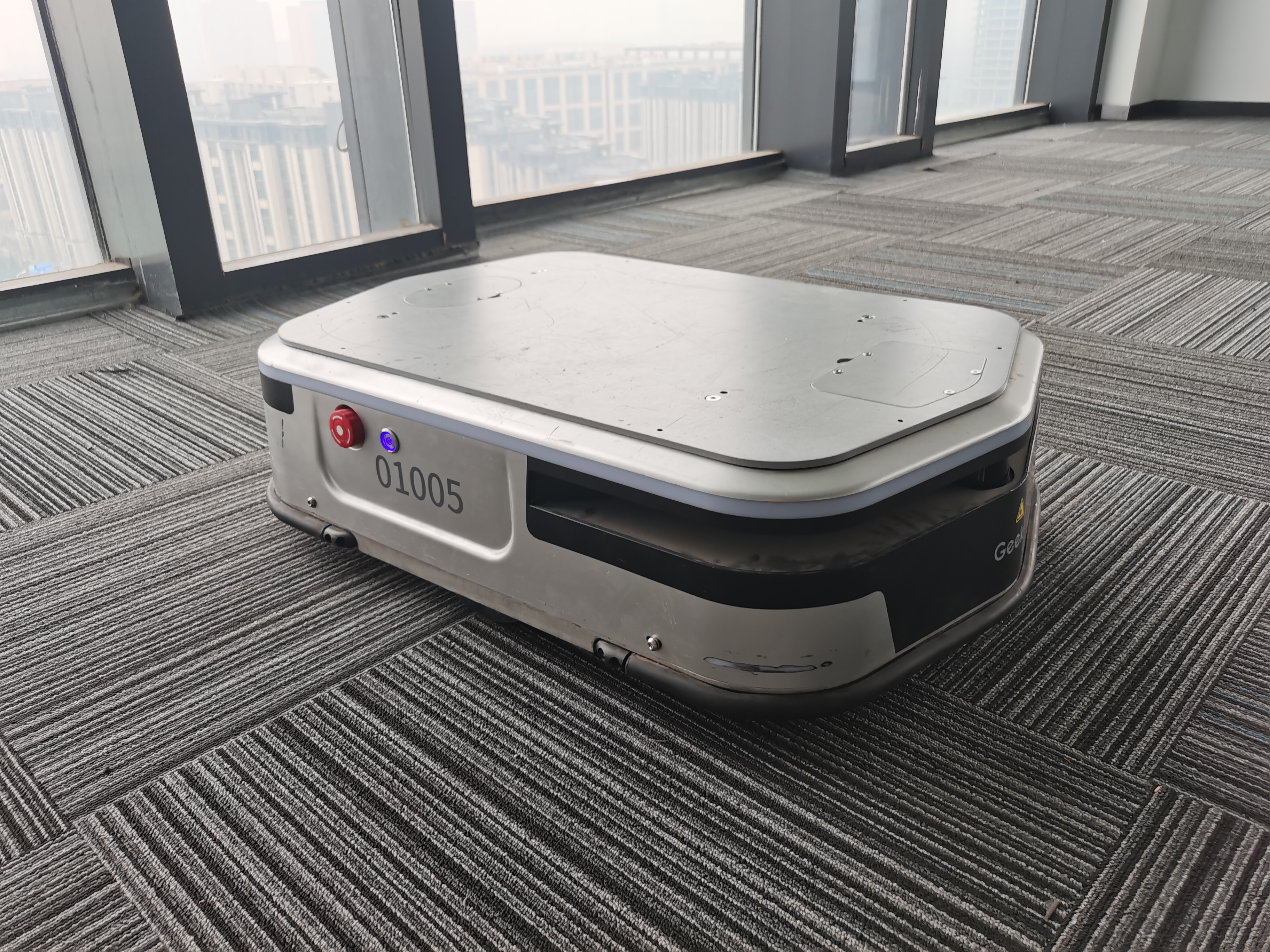
(a)

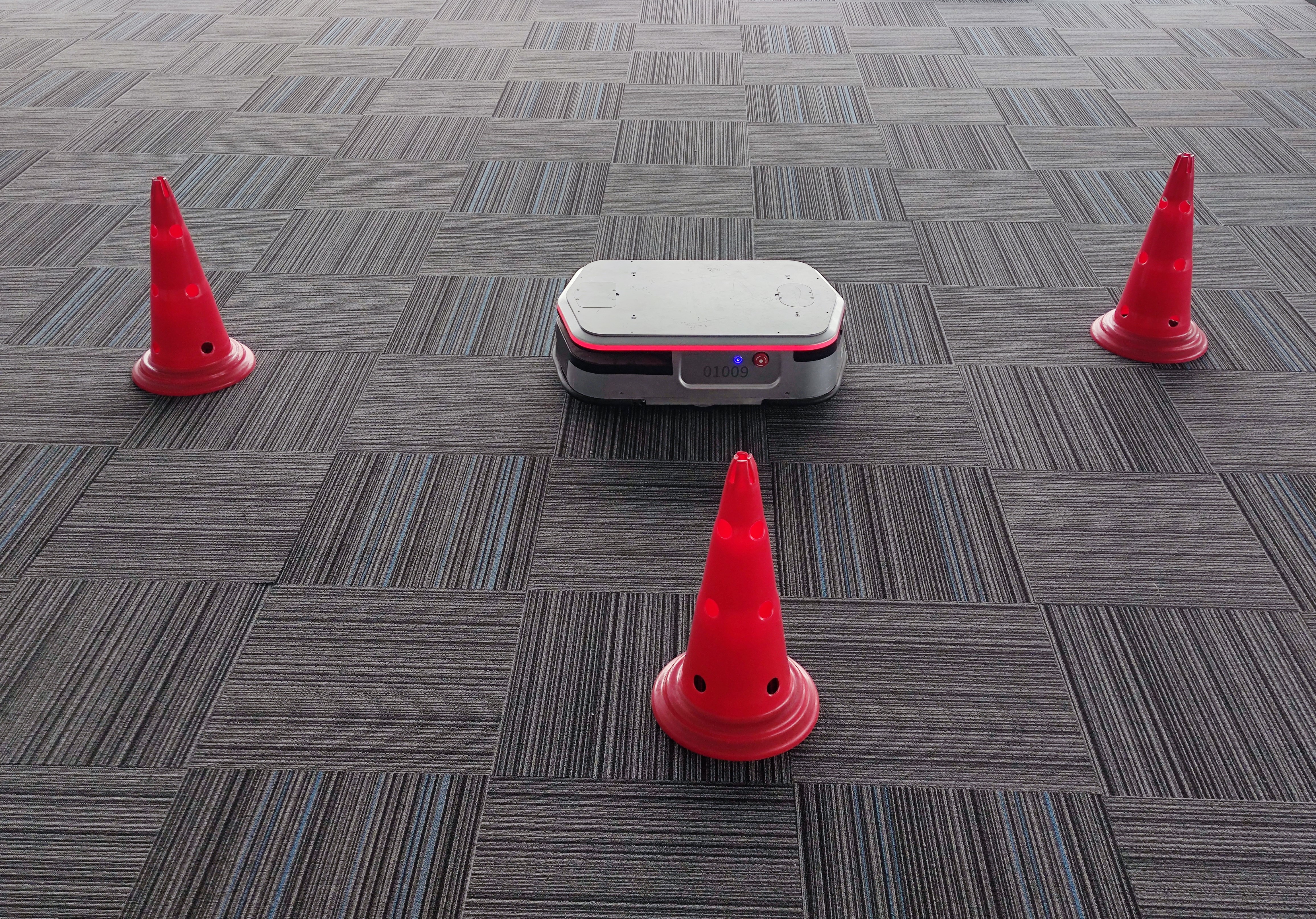
(b)

Figure 6: (a) The warehouse vehicle. (b) Experiment field. The three red traffic cones serve as landmarks for positioning.

The dynamics of the vehicle can be modeled as:

$$\begin{bmatrix}p_{x,t+1}\\ p_{y,t+1}\\ \theta_{t+1}\end{bmatrix}=\begin{bmatrix}p_{x,t}\\ p_{y,t}\\ \theta_{t}\end{bmatrix}+\begin{bmatrix}v_{t}\cdot\cos\theta_{t}\\ v_{t}\cdot\sin\theta_{t}\\ \omega_{t}\end{bmatrix}\cdot\Delta t+\xi_{t},$$ (24)

where $\Delta t=0.0667s$ is the sample period, $v_{t}$ is the longitudinal velocity, $\omega_{t}$ is the yaw rate, and $\xi_{t}$ is the process noise. In addition, the vehicle relies on three red traffic cones with predetermined positions as landmarks on the map to estimate its own location. The observation model is given by:

$$y_{t}=[d^{1}_{t},d^{2}_{t},d^{3}_{t},\alpha^{1}_{t},\alpha^{2}_{t},\alpha^{3}_{t}]^{\top}+\zeta_{t},$$ (25)

where $d^{i}$ and $\alpha^{i}$ ($i=1,2,3$) are defined as relative distance and orientation angle between the vehicle and the traffic cones respectively:

$$d^{i} =\|(p^{tc,i}_{x}-p_{x}-l\cos\theta,p^{tc,i}_{y}-p_{y}-l\sin\theta)\|_{2},$$ (26)

$$\alpha^{i} =\arctan\left(\frac{p^{tc,i}_{y}-p_{y}-l\sin\theta}{p^{tc,i}_{x}-p_{x}-l\cos\theta}\right)-\theta.$$

Here $(p^{tc,i}{x},p^{tc,i}{y})$ is the position of the $i_{\text{th}}$ traffic cone, and $l$ represents the longitudinal installation offset of the Lidar with respect to the robot center. The system model is illustrated in Fig. 7.

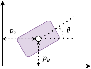
(a)

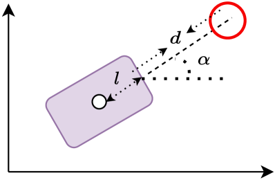
(b)

Figure 7: (a) The diagram of the vehicle’s states containing the 2D position of the vehicle $p_{x}$ and $p_{y}$, and the orientation angle $\theta$. (b) The diagram of the measurement model. Note that the red circle represents the red traffic cone.

We use an auxiliary high-definition indoor SLAM system to acquire highly precise location estimates for the vehicle, with a localization error less than $10mm$. The output of the SLAM system is treated as the ground truth states for evaluation. The detailed parameters about the experimental setup are given in Table 1.

Table 1: Parameters of the experiments.

Symbol	Description	Value
$(p^{lm}_{x,1},p^{lm}_{y,1})$	$1\text{st}$ traffic cone’s position	(1.05m, -2.69m)
$(p^{lm}_{x,2},p^{lm}_{y,2})$	$2\text{nd}$ traffic cone’s position	(4.07m, -1.75m)
$(p^{lm}_{x,3},p^{lm}_{y,3})$	$3\text{rd}$ traffic cone’s position	(6.02m, -3.32m)
$l$	Lidar longitude offset	0.329m

8.2 Data Pre-processing and Experimental Results

The experiment begins with the gathering of raw data, including ground truth states, control inputs, and the Lidar point cloud. Subsequently, we process the Lidar point cloud to extract measurements, which represent the relative distance and orientation angle between the vehicle and the traffic cones. The assembled dataset incorporates trajectories totaling 11 minutes in length.

Following this, we undertake the noise identification process, where we employ the ground truth data and measurements to obtain the parameters of the noise distribution. We operate under the assumption that both process and observation noises adhere to a Gaussian distribution, with each component being mutually independent. Specifically, the variance matrix of the Gaussian distribution manifests as a diagonal matrix. The noises can be represented as

$$\xi_{t}\sim\mathcal{N}\left(\mu_{\xi},\Sigma_{\xi}\right),\zeta_{t}\sim\mathcal{N}\left(\mu_{\zeta},\Sigma_{\zeta}\right).$$ (27)

For the acquired samples of process noise and measurement noise, we utilize (28) to implement a maximum likelihood estimation to identify the mean and variance of the distributions.

$$\xi_{t} =\begin{bmatrix}p_{x,t+1}\\ p_{y,t+1}\\ \theta_{t+1}\end{bmatrix}-\begin{bmatrix}p_{x,t}\\ p_{y,t}\\ \theta_{t}\end{bmatrix}-\begin{bmatrix}v_{t}\cdot\cos\theta_{t}\\ v_{t}\cdot\sin\theta_{t}\\ \omega_{t}\end{bmatrix}\cdot\Delta t,$$ (28)

$$\zeta_{t} =y_{t}-[d^{1}_{t},d^{2}_{t},d^{3}_{t},\alpha^{1}_{t},\alpha^{2}_{t},\alpha^{3}_{t}]^{\top}.$$

The identified parameters of the noise are:

$$\mu_{\xi} =\left[\begin{matrix}-0.00017&-0.00020&-0.00056\end{matrix}\right]^{\top},$$

$$\Sigma_{\xi} =\text{diag}\Big{(}\left[\begin{matrix}0.0034&0.0056&0.0041\end{matrix}\right]\Big{)},$$

$$\mu_{\zeta} =\left[\begin{matrix}-0.0312&-0.0581&-0.0557&0.0053&0.0059&0.0125\end{matrix}\right]^{\top},$$

$$\Sigma_{\zeta} =\text{diag}\Big{(}\left[\begin{matrix}0.0238&0.0284&0.0259&0.0107&0.0094&0.0118\end{matrix}\right]\Big{)}.$$

In the experiment, we simulate a scenario where the Lidar sensor might occasionally penetrate objects, thereby generating an output equivalent to the maximum Lidar range of 20m. Assuming that such an outlier is encountered with a probability of $p_{c}=0.01$, we segment the dataset into 50 sub-trajectories, each lasting 6.67 seconds (equivalent to 100 time steps). The experimental results are presented in Fig. 8 and Fig. 9, which provide a comparative analysis of the performance metrics of the UKF, MHE, and $\beta$-MHE under different $\beta$ values. The experimental results indicate that $\beta$-MHE yields superior performance than both MHE and UKF across various $\beta$ values.

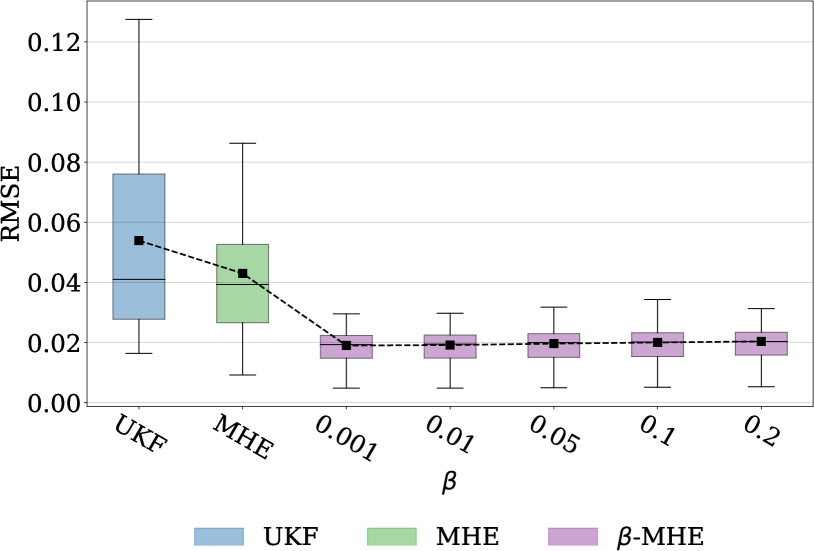
Figure 8: Box plot of RMSE for UKF, MHE and $\beta$-MHE with different values of $\beta$ when contamination probability $p_{c}=0.05$. The black square “ $\blacksquare$ ” represents the average RMSE.

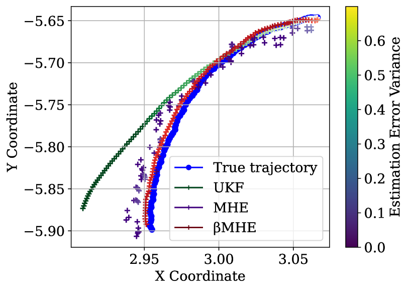
Figure 9: Robot trajectories with estimation error variance for UKF, MHE and $\beta$-MHE with $\beta=0.1$.

9 Conclusion

In this paper, we proposed a robust Bayesian inference framework for MHE that can maintain its accuracy in the presence of measurement outliers. By introducing a robust divergence measure, which assigns greater weight to inliers, our method mitigates the impact of outliers and significantly improves the robustness of the MHE method. We derived the analytical form of the influence functions for MHE methods. We demonstrated that, for linear Gaussian systems, the influence function of our proposed method is bounded, highlighting its robustness. Moreover, we performed stability analysis and shown that our proposed method exhibits robust asymptotic stability under certain conditions. Future studies will focus on developing techniques for auto-tuning parameters and applications to large-scale systems.

Appendix A Proof of Theorem 1

Proof.

Consider that the measurement model is contaminated by outliers, and the empirical probability satisfies

$$p_{\text{em}}^{t}(y)=(1-\epsilon)\delta(y-y_{t})+\epsilon\delta(y-z).$$ (29)

Substituting (29) for $p^{t}_{\text{true}}(y)$ in (10), the loss function $\ell^{\beta}(x_{t},y_{t})$ defined in (11) is converted to

$$\ell^{\beta,z,\epsilon}(x_{t},y_{t}) =-\frac{(1-\epsilon)(\beta+1)}{\beta}g(y_{t}|x_{t})^{\beta}$$

$$-\frac{\epsilon(\beta+1)}{\beta}g(z|x_{t})^{\beta}+\int{g(y|x_{t})^{\beta+1}\mathrm{d}y}.$$

If we replace $G^{\beta}(y_{t}|x_{t})$ defined in (12) with $G^{\beta,z,\epsilon}(y_{t}|x_{t}):=\exp{\left(-\ell^{\beta,z,\epsilon}(x_{t},y_{t})\right)}$, the state estimate with contaminated data can be obtained by

$$\hat{x}_{t-T:t}^{z,\epsilon}=\arg\min_{x_{t-T:t}}\left\{J^{\beta,z,\epsilon}(x_{t-T:t})\right\},$$

where

$$J^{\beta,z,\epsilon}(x_{t-T:t})$$

$$=\Gamma(x_{t-T})+\sum\limits_{i=t-T+1}^{t}\left\{k(x_{i},x_{i-1})+\ell^{\beta,z,\epsilon}(x_{i},y_{i})\right\}.$$

Here $\Gamma(x_{t-T})$ satisfies (5a), and $k(x_{t},x_{t-1})$ satisfies (5b). By the assumption of the differentiability of $J^{\beta,z,\epsilon}(x_{t-T:t})$, we obtain

$$\left.\frac{\partial{\left\{J^{\beta,z,\epsilon}(x_{t-T:t})\right\}}}{\partial{x_{t-T:t}}}\right|_{x_{t-T:t}=\hat{x}_{t-T:t}^{z,\epsilon}}=0.$$ (30)

According to the definition,

$$\mathbb{IF}(z,\hat{x}_{t-T:t},G^{\beta}(y_{t}|x_{t}))=\left.\frac{\partial{\hat{x}_{t-T:t}^{z,\epsilon}}}{\partial{\epsilon}}\right|_{\epsilon=0}.$$

Taking the derivative of the both sides of (30) with respect to $\epsilon$ at $\epsilon=0$ and defining $\mathscr{K}^{\beta,z}(x_{t},y_{t})=\left.\frac{\partial{\ell^{\beta,z,\epsilon}(x_{t},y_{t})}}{\partial{\epsilon}}\right|_{\epsilon=0}$, we have

$$\left.\frac{\partial^{2}{\left[J(x_{t-T:t})\right]}}{\partial{x_{t-T:t}^{2}}}\right|_{{x_{t-T:t}=\hat{x}_{t-T:t}}}\cdot\mathbb{IF}(z,\hat{x}_{t-T:t},G^{\beta}(y_{t}|x_{t}))$$

$$+\sum\limits_{i=t-T+1}^{t}\left.\frac{\partial{\left[\mathscr{K}^{\beta,z}(x_{i},y_{i})\right]}}{\partial{x_{t-T:t}}}\right|_{{x_{t-T:t}=\hat{x}_{t-T:t}}}=0.$$

Here, $J(x_{t-T:t})$ is defined by (4b)(5a)(5b)(13). Therefore, (14a) holds given the Assumption 2 that the Hessian matrix $M_{1}(\hat{x}_{t-T:t})$ is nonsingular. ∎

Appendix B Proof of Theorem 2

Proof.

First, we will prove that the gross error sensitivity of MHE is infinite. We observe that

$$\|M_{2}(z,\hat{x}_{t-T:t})\|\leq\|M_{1}(\hat{x}_{t-T:t})\|_{\mathcal{F}}\cdot\|\mathbb{IF}(z,\hat{x}_{t-T:t},g(y_{t}|x_{t}))\|.$$

For MHE, we have

$$\sum\limits_{j=t-T+1}^{t}\left.\frac{\partial{\left[\mathscr{K}^{z}(x_{j},y_{j})\right]}}{\partial{x_{t-T}}}\right|_{x_{t-T}=\hat{x}_{t-T}}=0,$$ (31)

and

$$\sum\limits_{j=t-T+1}^{t}\left.\frac{\partial{\left[\mathscr{K}^{z}(x_{j},y_{j})\right]}}{\partial{x_{t-i}}}\right|_{x_{t-i}=\hat{x}_{t-i}}=C^{\top}R^{-1}(y_{t-i}-C\hat{x}_{t-i})$$ (32)

$$-C^{\top}R^{-1}(z-C\hat{x}_{t-i}),\;\;i\in\mathbb{Z}_{[0,T-1]}.$$

Thus $\sup_{z}\|M_{2}(z,\hat{x}_{t-T:t})\|=\infty$, which leads to

$$\gamma(\hat{x}_{t-T:t},g(y_{t}|x_{t})) =\sup_{z}{\|\mathbb{IF}(z,\hat{x}_{t-T:t},g(y_{t}|x_{t}))\|}$$

$$\geq\frac{\sup_{z}\|M_{2}(z,\hat{x}_{t-T:t})\|}{\|M_{1}(\hat{x}_{t-T:t})\|_{\mathcal{F}}}$$

$$=\infty.$$

In the next step, we will prove that the gross error sensitivity of the $\beta$-MHE is bounded. We find

$$\|\mathbb{IF}(z,\hat{x}_{t-T:t},G^{\beta}(y_{t}|x_{t}))\|\leq \|M_{1}^{-1}(\hat{x}_{t-T:t})\|_{\mathcal{F}}$$

$$\cdot \|M_{2}(z,\hat{x}_{t-T:t})\|.$$

Similar to (31) and (32), we have

$$\sum\limits_{j=t-T+1}^{t}\left.\frac{\partial{\left[\mathscr{K}^{\beta,z}(x_{j},y_{j})\right]}}{\partial{x_{t-T}}}\right|_{x_{t-T}=\hat{x}_{t-T}}=0,$$

and

$$\sum\limits_{j=t-T+1}^{t}\left.\frac{\partial{\left[\mathscr{K}^{\beta,z}(x_{j},y_{j})\right]}}{\partial{x_{t-i}}}\right|_{x_{t-i}=\hat{x}_{t-i}}$$

$$=\frac{(\beta+1)C^{\top}R^{{-}1}}{\sqrt{(2\pi)^{\beta m}|R|^{\beta}}}(y_{t-i}-C\hat{x}_{t-i})e^{-\frac{\beta}{2}\|y_{t-i}-C\hat{x}_{t-i}\|^{2}_{{R}^{-1}}}$$

$$-\frac{(\beta+1)C^{\top}R^{-1}}{\sqrt{(2\pi)^{\beta m}|R|^{\beta}}}(z-C\hat{x}_{t-i})e^{-\frac{\beta}{2}\|z-C\hat{x}_{t-i}\|^{2}_{{R}^{-1}}},$$

$$\forall i\in\mathbb{Z}_{[0,T-1]}.$$

Define the function $\rho(\hat{x}_{t},z)$ as in (19) and we observe that $\lim_{z\to\infty}\rho(\hat{x}_{t},z)=0$. Because $\|\rho(\hat{x}_{t},z)\|^{2}$ is continuous with respect to $z$, it is bounded, i.e.,

$$\|\rho(\hat{x}_{t},z)\|\leq \rho_{\text{max}},\;\;\forall z.$$

Because

$$\|M_{2}(z,\hat{x}_{t-T:t})\|^{2}$$

$$=\sum\limits_{i=0}^{T-1}\left\|\sum\limits_{j=t-T+1}^{t}\left.\frac{\partial{\left[\mathcal{K}^{\beta,z}(x_{j},y_{j})\right]}}{\partial{x_{t-i}}}\right|_{x_{t-i}=\hat{x}_{t-i}}\right\|^{2}$$

$$\leq 4T\cdot\rho_{\text{max}}^{2},$$

we get

$$\|\mathbb{IF}(z,\hat{x}_{t-T:t},G^{\beta}(y_{t}|x_{t}))\| \leq 2\sqrt{T}\cdot\|M_{1}^{-1}(\hat{x}_{t-T:t})\|_{\mathcal{F}}\cdot\rho_{\text{max}}.$$ (33)

Taking the supremum on both sides of (33) results in (18), thereby completing the proof. ∎

Appendix C Proof of Theorem 3

In order to prove the robust stability of MHE, we first need a proposition that bounds the estimator error within the MHE problem in terms of the initial state estimate error and the norm of disturbances.

Proposition 1.

Under Assumption 1, for $\forall t\in\mathbb{Z}_{[0,T]}$, we have

$$\|\hat{x}_{t|t}-x_{t}\|$$ (34)

$$\leq \gamma_{x}\left(2\sqrt{3}\cdot\|{x}_{0}-\hat{x}_{0|0}\|,t\right)\oplus\gamma_{x}\left(2\sqrt{\frac{3T}{\mu}\cdot\bar{\gamma}_{\xi}\left(\|\xi\|_{0:t-1}\right)},t\right)$$

$$\oplus \gamma_{x}\left(2\sqrt{\frac{3T}{\mu}\cdot\bar{\gamma}_{\zeta}\left(\|\zeta\|_{1:t}\right)},t\right)\oplus\gamma_{\xi}\left(2\underline{\gamma}_{\xi}^{-1}\Big{(}3\mu\cdot\|{x}_{0}-\hat{x}_{0|0}\|^{2}\Big{)}\right)$$

$$\oplus \gamma_{\xi}\left(2\underline{\gamma}_{\xi}^{-1}\Big{(}3T\cdot\bar{\gamma}_{\xi}\left(\|\xi\|_{0:t-1}\right)\Big{)}\right)\oplus\gamma_{\xi}\left(2\underline{\gamma}_{\xi}^{-1}\Big{(}3T\cdot\bar{\gamma}_{\zeta}\left(\|\zeta\|_{1:t}\right)\Big{)}\right)$$

$$\oplus \gamma_{\zeta}\left(2\underline{\gamma}_{\zeta}^{-1}\Big{(}3\mu\cdot\|{x}_{0}-\hat{x}_{0|0}\|^{2}\Big{)}\right)\oplus\gamma_{\zeta}\left(2\underline{\gamma}_{\zeta}^{-1}\Big{(}3T\cdot\bar{\gamma}_{\xi}\left(\|\xi\|_{0:t-1}\right)\Big{)}\right)$$

$$\oplus \gamma_{\zeta}\left(2\underline{\gamma}_{\zeta}^{-1}\Big{(}3T\cdot\bar{\gamma}_{\zeta}\left(\|\zeta\|_{1:t}\right)\Big{)}\right).$$

Proof.

By Assumption 1, the MHE problem exists a solution $\hat{x}_{0|t},\hat{\xi}_{0:t-1|t},\hat{\zeta}_{1:t|t}$. For $\forall t\in\mathbb{Z}_{[0,T]}$, we have

$$\mu\cdot\|\hat{x}_{0|t}-\hat{x}_{0|0}\|^{2}\oplus\underline{\gamma}_{\xi}\left(\|\hat{\xi}\|_{0:t-1}\right)\oplus\underline{\gamma}_{\zeta}\left(\|\hat{\zeta}\|_{1:t}\right)$$

$$\leq \mu\cdot\|\hat{x}_{0|t}-\hat{x}_{0|0}\|^{2}+\underline{\gamma}_{\xi}\left(\|\hat{\xi}\|_{0:t-1}\right)+\underline{\gamma}_{\zeta}\left(\|\hat{\zeta}\|_{1:t}\right)$$

$$\leq J(\hat{x}_{0|t},\hat{\xi}_{0:t-1|t})$$

$$\leq J(\hat{x}_{0|t},{\xi}_{0:t-1|t})$$

$$\leq 3\mu\cdot\|{x}_{0}-\hat{x}_{0|0}\|^{2}\oplus 3T\cdot\bar{\gamma}_{\xi}\left(\|\xi\|_{0:t-1}\right)\oplus 3T\cdot\bar{\gamma}_{\zeta}\left(\|\zeta\|_{1:t}\right).$$

Thus, we obtain the following bounds

$$\|\hat{x}_{0|t}-\hat{x}_{0|0}\|$$

$$\leq\frac{\sqrt{3}}{\sqrt{\mu}}\Big{(}\sqrt{\mu\cdot\|{x}_{0}-\hat{x}_{0|0}\|^{2}\oplus T\cdot\bar{\gamma}_{\xi}\left(\|\xi\|_{0:t-1}\right)\oplus T\cdot\bar{\gamma}_{\zeta}\left(\|\zeta\|_{1:t}\right)}\Big{)}$$

$$=\sqrt{3}\cdot\|{x}_{0}-\hat{x}_{0|0}\|\oplus\sqrt{\frac{3T}{\mu}\cdot\bar{\gamma}_{\xi}\left(\|\xi\|_{0:t-1}\right)}\oplus\sqrt{\frac{3T}{\mu}\cdot\bar{\gamma}_{\zeta}\left(\|\zeta\|_{1:t}\right)},$$ (35a)

$$\|\hat{\xi}\|_{0:t-1}$$

$$\leq\underline{\gamma}_{\xi}^{-1}\Big{(}3\Big{(}\mu\cdot\|{x}_{0}-\hat{x}_{0|0}\|^{2}\oplus T\cdot\bar{\gamma}_{\xi}\left(\|\xi\|_{0:t-1}\right)\oplus T\cdot\bar{\gamma}_{\zeta}\left(\|\zeta\|_{1:t}\right)\Big{)}\Big{)}$$

$$=\underline{\gamma}_{\xi}^{-1}\Big{(}3\mu\cdot\|{x}_{0}-\hat{x}_{0|0}\|^{2}\Big{)}\oplus\underline{\gamma}_{\xi}^{-1}\Big{(}3T\cdot\bar{\gamma}_{\xi}\left(\|\xi\|_{0:t-1}\right)\Big{)}$$

$$\oplus\underline{\gamma}_{\xi}^{-1}\Big{(}3T\cdot\bar{\gamma}_{\zeta}\left(\|\zeta\|_{1:t}\right)\Big{)},$$ (35b)

$$\|\hat{\zeta}\|_{1:t}$$

$$\leq\underline{\gamma}_{\zeta}^{-1}\Big{(}3\Big{(}\mu\cdot\|{x}_{0}-\hat{x}_{0|0}\|^{2}\oplus T\cdot\bar{\gamma}_{\xi}\left(\|\xi\|_{0:t-1}\right)\oplus T\cdot\bar{\gamma}_{\zeta}\left(\|\zeta\|_{1:t}\right)\Big{)}\Big{)}$$

$$=\underline{\gamma}_{\zeta}^{-1}\Big{(}3\mu\cdot\|{x}_{0}-\hat{x}_{0|0}\|^{2}\Big{)}\oplus\underline{\gamma}_{\zeta}^{-1}\Big{(}3T\cdot\bar{\gamma}_{\xi}\left(\|\xi\|_{0:t-1}\right)\Big{)}$$

$$\oplus\underline{\gamma}_{\zeta}^{-1}\Big{(}3T\cdot\bar{\gamma}_{\zeta}\left(\|\zeta\|_{1:t}\right)\Big{)}.$$ (35c)

From the system’s i-IOSS bound in (20), we have

$$\|\hat{x}_{t|t}-x_{t}\|$$ (36)

$$\leq \gamma_{x}(\|\hat{x}_{0|t}-x_{0}\|,t)\oplus\gamma_{\xi}\left(\|{\xi}-\hat{\xi}\|_{0:t-1}\right)\oplus\gamma_{\zeta}\left(\|\zeta-\hat{\zeta}\|_{1:t}\right)$$

$$\leq \gamma_{x}(\|\hat{x}_{0|t}-\hat{x}_{0|0}+\hat{x}_{0|0}-x_{0}\|,t)$$

$$\oplus \gamma_{\xi}(\left\|{\xi}\right\|_{0:t-1}+|\hat{\xi}\|_{0:t-1})\oplus\gamma_{\zeta}\left(\|{\zeta}\|_{1:t}+\|\hat{\zeta}\|_{1:t}\right)$$

$$\leq \gamma_{x}(2\|\hat{x}_{0|t}-\hat{x}_{0|0}\|\oplus 2|\hat{x}_{0|0}-x_{0}|,t)$$

$$\oplus \gamma_{\xi}(2\left\|{\xi}\right\|_{0:t-1}\oplus 2\|\hat{\xi}\|_{0:t-1})\oplus\gamma_{\zeta}(2\|{\zeta}\|_{1:t}\oplus 2\|\hat{\zeta}\|_{1:t}).$$

Substituting (35) into (36), we have

$$\|\hat{x}_{t|t}-x_{t}\|$$

$$\leq \gamma_{x}(2\|\hat{x}_{0|t}-\hat{x}_{0|0}\|\oplus 2\|\hat{x}_{0|0}-x_{0}\|,t)$$

$$\oplus \gamma_{\xi}(2\left\|{\xi}\right\|_{0:t-1}\oplus 2\|\hat{\xi}\|_{0:t-1})\oplus\gamma_{\zeta}(2\|{\zeta}\|_{1:t}\oplus 2\|\hat{\zeta}\|_{1:t})$$

$$\leq \gamma_{x}(2\|\hat{x}_{0|0}-x_{0}\|,t)\oplus\gamma_{\xi}(2\left\|{\xi}\right\|_{0:t-1})\oplus\gamma_{\zeta}(2\left\|{\zeta}\right\|_{1:t})$$

$$\oplus \gamma_{x}\left(2\sqrt{3}\cdot\|{x}_{0}-\hat{x}_{0|0}\|,t\right)\oplus\gamma_{x}\left(2\sqrt{\frac{3T}{\mu}\cdot\bar{\gamma}_{\xi}\left(\|\xi\|_{0:t-1}\right)},t\right)$$

$$\oplus \gamma_{x}\left(2\sqrt{\frac{3T}{\mu}\cdot\bar{\gamma}_{\zeta}\left(\|\zeta\|_{1:t}\right)},t\right)\oplus\gamma_{\xi}\left(2\underline{\gamma}_{\xi}^{-1}\Big{(}3\mu\cdot\|{x}_{0}-\hat{x}_{0|0}\|^{2}\Big{)}\right)$$

$$\oplus \gamma_{\xi}\left(2\underline{\gamma}_{\xi}^{-1}\Big{(}3T\cdot\bar{\gamma}_{\xi}\left(\|\xi\|_{0:t-1}\right)\Big{)}\right)\oplus\gamma_{\xi}\left(2\underline{\gamma}_{\xi}^{-1}\Big{(}3T\cdot\bar{\gamma}_{\zeta}\left(\|\zeta\|_{1:t}\right)\Big{)}\right)$$

$$\oplus \gamma_{\zeta}\left(2\underline{\gamma}_{\zeta}^{-1}\Big{(}3\mu\cdot\|{x}_{0}-\hat{x}_{0|0}\|^{2}\Big{)}\right)\oplus\gamma_{\zeta}\left(2\underline{\gamma}_{\zeta}^{-1}\Big{(}3T\cdot\bar{\gamma}_{\xi}\left(\|\xi\|_{0:t-1}\right)\Big{)}\right)$$

$$\oplus \gamma_{\zeta}\left(2\underline{\gamma}_{\zeta}^{-1}\Big{(}3T\cdot\bar{\gamma}_{\zeta}\left(\|\zeta\|_{1:t}\right)\Big{)}\right).$$

Combine with the fact that

$$\gamma_{x}(2\|\hat{x}_{0|0}-x_{0}\|,t) \leq\gamma_{x}\left(2\sqrt{3}\cdot\|{x}_{0}-\hat{x}_{0|0}\|,t\right),$$

$$\gamma_{\xi}(2\left\|{\xi}\right\|_{0:t-1}) \leq\gamma_{\xi}\left(2\underline{\gamma}_{\xi}^{-1}\Big{(}3T\cdot\bar{\gamma}_{\xi}\left(\|\xi\|_{0:t-1}\right)\Big{)}\right),$$

$$\gamma_{\zeta}(2\left\|{\zeta}\right\|_{1:t}) \leq\gamma_{\zeta}\left(2\underline{\gamma}_{\zeta}^{-1}\Big{(}3T\cdot\bar{\gamma}_{\zeta}\left(\|\zeta\|_{1:t}\right)\Big{)}\right),$$

we can finally obtain (34). ∎

Then, we give the proof of Theorem 3.

Proof.

By Proposition 1, we have

$$\|\hat{x}_{t+T|t+T}-x_{t+T}\|$$ (37)

$$\leq \gamma_{x}\left(2\sqrt{3}\cdot\|{x}_{t}-\hat{x}_{t|t}\|,T\right)\oplus\gamma_{x}\left(2\sqrt{\frac{3T}{\mu}\cdot\bar{\gamma}_{\xi}\left(\|\xi\|_{t:t+T-1}\right)},T\right)$$

$$\oplus \gamma_{x}\left(2\sqrt{\frac{3T}{\mu}\cdot\bar{\gamma}_{\zeta}\left(\|\zeta\|_{t+1:t+T}\right)},T\right)\oplus\gamma_{\xi}\left(2\underline{\gamma}_{\xi}^{-1}\Big{(}3\mu\cdot\|{x}_{t}-\hat{x}_{t|t}\|^{2}\Big{)}\right)$$

$$\oplus \gamma_{\xi}\left(2\underline{\gamma}_{\xi}^{-1}\Big{(}3T\cdot\bar{\gamma}_{\xi}\left(\|\xi\|_{t:t+T-1}\right)\Big{)}\right)\oplus\gamma_{\xi}\left(2\underline{\gamma}_{\xi}^{-1}\Big{(}3T\cdot\bar{\gamma}_{\zeta}\left(\|\zeta\|_{t+1:t+T}\right)\Big{)}\right)$$

$$\oplus \gamma_{\zeta}\left(2\underline{\gamma}_{\zeta}^{-1}\Big{(}3\mu\cdot\|{x}_{t}-\hat{x}_{t|t}\|^{2}\Big{)}\right)\oplus\gamma_{\zeta}\left(2\underline{\gamma}_{\zeta}^{-1}\Big{(}3T\cdot\bar{\gamma}_{\xi}\left(\|\xi\|_{t:t+T-1}\right)\Big{)}\right)$$

$$\oplus \gamma_{\zeta}\left(2\underline{\gamma}_{\zeta}^{-1}\Big{(}3T\cdot\bar{\gamma}_{\zeta}\left(\|\zeta\|_{t+1:t+T}\right)\Big{)}\right).$$

Define the $\mathcal{K}$ functions $\alpha_{\xi}(s)$ and $\alpha_{\zeta}(s)$ as:

$$\alpha_{\xi}(s) :=\gamma_{x}\left(2\sqrt{\frac{3T}{\mu}\cdot\bar{\gamma}_{\xi}\left(s\right)},0\right)$$

$$\oplus\gamma_{\xi}\left(2\underline{\gamma}_{\xi}^{-1}\Big{(}3T\cdot\bar{\gamma}_{\xi}\left(s\right)\Big{)}\right)\oplus\gamma_{\zeta}\left(2\underline{\gamma}_{\zeta}^{-1}\Big{(}3T\cdot\bar{\gamma}_{\xi}\left(s\right)\Big{)}\right),$$

$$\alpha_{\zeta}(s) :=\gamma_{x}\left(2\sqrt{\frac{3T}{\mu}\cdot\bar{\gamma}_{\zeta}\left(s\right)},0\right)$$

$$\oplus\gamma_{\xi}\left(2\underline{\gamma}_{\xi}^{-1}\Big{(}3T\cdot\bar{\gamma}_{\zeta}\left(s\right)\Big{)}\right)\oplus\gamma_{\zeta}\left(2\underline{\gamma}_{\zeta}^{-1}\Big{(}3T\cdot\bar{\gamma}_{\zeta}\left(s\right)\Big{)}\right).$$

Define $\lambda:=2\sqrt{3}\eta<1$, for $\eta\in(0,\frac{1}{2\sqrt{3}})$, by Assumption 3, for $\|x_{t}-\hat{x}_{t|t}\|\leq\bar{s}$, there exists $T\geq T_{m}\geq 0$, such that

$$\gamma_{x}(2\sqrt{3}\cdot\|{x}_{t}-\hat{x}_{t|t}\|,T) \leq\gamma_{x}(2\sqrt{3}\cdot\|{x}_{t}-\hat{x}_{t|t}\|,T_{m})$$

$$\leq 2\sqrt{3}\eta\|{x}_{t}-\hat{x}_{t|t}\|$$

$$=\lambda|{x}_{t}-\hat{x}_{t|t}|.$$

Note that there exists $\delta>0$ such that if $\|\xi\|_{0:\infty},\|\zeta\|_{0:\infty}\leq\delta$, then $\alpha_{\xi}(\|\xi\|_{0:\infty}),\alpha_{\zeta}(\|\zeta\|_{0:\infty})\leq\bar{s},\forall\bar{s}>0$. By Assumption 5, for $\|x_{t}-\hat{x}_{t|t}\|\leq\bar{s}$, we can make $\mu$ small enough, such that

$$\gamma_{\xi}\left(2\underline{\gamma}_{\xi}^{-1}\Big{(}3\mu\cdot\|{x}_{t}-\hat{x}_{t|t}\|^{2}\Big{)}\right)\leq\lambda\|{x}_{t}-\hat{x}_{t|t}\|,$$

$$\gamma_{\zeta}\left(2\underline{\gamma}_{\zeta}^{-1}\Big{(}3\mu\cdot\|{x}_{t}-\hat{x}_{t|t}\|^{2}\Big{)}\right)\leq\lambda\|{x}_{t}-\hat{x}_{t|t}\|.$$

Thus, from (37), we can obtain

$$\|\hat{x}_{t+T|t+T}-x_{t+T}\| \leq\lambda\|{x}_{t}-\hat{x}_{t|t}\|$$ (38)

$$\oplus\alpha_{\xi}(\|{\xi}\|_{t:t+T-1})\oplus\alpha_{\zeta}(\|{\zeta}\|_{t+1:t+T}),$$

for $\|x_{t}-\hat{x}_{t|t}\|\leq\bar{s}$.

By Proposition 1, for $i\leq T$, we have

$$\|\hat{x}_{i|i}-x_{i}\|$$ (39)

$$\leq \gamma_{x}\left(2\sqrt{3}\cdot\|{x}_{0}-\hat{x}_{0|0}\|,i\right)\oplus\gamma_{x}\left(2\sqrt{\frac{3T}{\mu}\cdot\bar{\gamma}_{\xi}\left(\|\xi\|_{0:i-1}\right)},i\right)$$

$$\oplus \gamma_{x}\left(2\sqrt{\frac{3T}{\mu}\cdot\bar{\gamma}_{\zeta}\left(\|\zeta\|_{1:i}\right)},i\right)\oplus\gamma_{\xi}\left(2\underline{\gamma}_{\xi}^{-1}\Big{(}3\mu\cdot\|{x}_{0}-\hat{x}_{0|0}\|^{2}\Big{)}\right)$$

$$\oplus \gamma_{\xi}\left(2\underline{\gamma}_{\xi}^{-1}\Big{(}3T\cdot\bar{\gamma}_{\xi}\left(\|\xi\|_{0:i-1}\right)\Big{)}\right)\oplus\gamma_{\xi}\left(2\underline{\gamma}_{\xi}^{-1}\Big{(}3T\cdot\bar{\gamma}_{\zeta}\left(\|\zeta\|_{1:i}\right)\Big{)}\right)$$

$$\oplus \gamma_{\zeta}\left(2\underline{\gamma}_{\zeta}^{-1}\Big{(}3\mu\cdot\|{x}_{0}-\hat{x}_{0|0}\|^{2}\Big{)}\right)\oplus\gamma_{\zeta}\left(2\underline{\gamma}_{\zeta}^{-1}\Big{(}3T\cdot\bar{\gamma}_{\xi}\left(\|\xi\|_{0:i-1}\right)\Big{)}\right)$$

$$\oplus \gamma_{\zeta}\left(2\underline{\gamma}_{\zeta}^{-1}\Big{(}3T\cdot\bar{\gamma}_{\zeta}\left(\|\zeta\|_{1:i}\right)\Big{)}\right).$$

Regarding the definition of $\alpha_{\xi},\alpha_{\zeta}$ and define the $\mathcal{K}$ function $\alpha_{x}$ as

$$\alpha_{x}(s)=\gamma_{x}(2\sqrt{3}s,0)\oplus\lambda s,$$

we have

$$\|x_{i}-\hat{x}_{i|i}\|\leq\alpha_{x}(\|x_{0}-\hat{x}_{0|0}\|)\oplus\alpha_{\xi}(\|{\xi}\|_{0:i-1})\oplus\alpha_{\zeta}(\|{\zeta}\|_{1:i}).$$

Next, we prove by induction that

$$\|\hat{x}_{i+jT|i+jT}-x_{i+jT}\|\leq\lambda^{j}\alpha_{x}(\|x_{0}-\hat{x}_{0|0}\|)$$ (40)

$$\oplus\alpha_{\xi}(\|{\xi}\|_{jT:jT+i-1})\oplus\alpha_{\zeta}(\|{\zeta}\|_{jT+1:jT+i})$$

$$\oplus\max_{0\leq k\leq j-1}\left\{\alpha_{\xi}(\lambda^{j-k-1}\|{\xi}\|_{kT:(k+1)T-1})\right\}$$

$$\oplus\max_{0\leq k\leq j-1}\left\{\alpha_{\zeta}(\lambda^{j-k-1}\|{\zeta}\|_{kT+1:(k+1)T})\right\},$$

for all $j\geq 0$ and $0\leq i\leq T-1$ with $\lambda<1$. The base is (40) and then we perform the inductive step. By applying (38), we have

$$\|\hat{x}_{i+(j+1)T|i+(j+1)T}-x_{i+(j+1)T}\|$$

$$\leq \lambda\|{x}_{i+jT}-\hat{x}_{i+jT|i+jT}\|\oplus\alpha_{\xi}(\|{\xi}\|_{i+jT:i+(j+1)T-1})$$

$$\oplus \alpha_{\zeta}(\|{\zeta}\|_{i+jT+1:i+(j+1)T})$$

$$\leq \lambda^{j+1}\alpha_{x}(\|x_{0}-\hat{x}_{0|0}\|)\oplus\lambda\alpha_{\xi}(\|{\xi}\|_{jT:jT+i-1})$$

$$\oplus \lambda\alpha_{\zeta}(\|{\zeta}\|_{jT+1:jT+i})\oplus\max_{0\leq k\leq j-1}\left\{\alpha_{\xi}(\lambda^{j-k}\|{\xi}\|_{kT:(k+1)T-1})\right\}$$

$$\oplus \max_{0\leq k\leq j-1}\left\{\alpha_{\zeta}(\lambda^{j-k}\|{\zeta}\|_{kT+1:(k+1)T})\right\}$$

$$\oplus \alpha_{\xi}(\|{\xi}\|_{i+jT:i+(j+1)T-1})\oplus\alpha_{\zeta}(\|{\zeta}\|_{i+jT+1:i+(j+1)T})$$

$$\leq \lambda^{j+1}\alpha_{x}(\|x_{0}-\hat{x}_{0|0}\|)\oplus\alpha_{\xi}(\|{\xi}\|_{jT:(j+1)T+i-1})$$

$$\oplus \alpha_{\zeta}(\|{\zeta}\|_{jT+1:(j+1)T+i})\oplus\max_{0\leq k\leq j-1}\left\{\alpha_{\xi}(\lambda^{j-k}\|{\xi}\|_{kT:(k+1)T-1})\right\}$$

$$\oplus \max_{0\leq k\leq j-1}\left\{\alpha_{\zeta}(\lambda^{j-k}\|{\zeta}\|_{kT+1:(k+1)T})\right\}$$

$$\leq \lambda^{j+1}\alpha_{x}(\|x_{0}-\hat{x}_{0|0}\|)\oplus\alpha_{\xi}(\|{\xi}\|_{(j+1)T:(j+1)T+i-1})$$

$$\oplus \alpha_{\zeta}(\|{\zeta}\|_{(j+1)T+1:(j+1)T+i})\oplus\max_{0\leq k\leq j}\left\{\alpha_{\xi}(\lambda^{j-k}\|{\xi}\|_{kT:(k+1)T-1})\right\}$$

$$\oplus \max_{0\leq k\leq j}\left\{\alpha_{\zeta}(\lambda^{j-k}\|{\zeta}\|_{kT+1:(k+1)T})\right\}.$$

which is the required statement. An immediate consequence of this statement is that

$$\|\hat{x}_{i+jT|i+jT}-x_{i+jT}\|$$

$$\leq \lambda^{j}\alpha_{x}(\|x_{0}-\hat{x}_{0|0}\|)\oplus\alpha_{\xi}(\|{\xi}\|_{0:jT+i-1})\oplus\alpha_{\zeta}(\|{\zeta}\|_{1:jT+i}),$$

for all $0\leq i\leq T-1$ and $j\geq 0$. For $t=jT+i$, define the $\mathcal{KL}$ function $\rho_{x}(s,t):=\lambda^{\lfloor{t/T}\rfloor}\alpha_{x}(s),\rho_{\xi}=\alpha_{\xi},\rho_{\zeta}=\alpha_{\zeta}$, thus we have

$$|x_{t}-\hat{x}_{t|t}|\leq\rho_{x}(\|x_{0}-\hat{x}_{0|0}\|,t)\oplus\rho_{\xi}(\|{\xi}\|_{0:t-1})\oplus\rho_{\zeta}(\|{\zeta}\|_{1:t}).$$

∎

References

- [1] Haleh Akrami, Anand A Joshi, Jian Li, Sergül Aydöre, and Richard M Leahy. A robust variational autoencoder using beta divergence. Knowledge-Based Systems, 238:107886, 2022.
- [2] Angelo Alessandri and Moath Awawdeh. Moving-horizon estimation for discrete-time linear systems with measurements subject to outliers. In 53rd IEEE Conference on Decision and Control, pages 2591–2596. IEEE, 2014.
- [3] Angelo Alessandri and Moath Awawdeh. Moving-horizon estimation with guaranteed robustness for discrete-time linear systems and measurements subject to outliers. Automatica, 67:85–93, 2016.
- [4] Douglas A Allan and James B Rawlings. Moving horizon estimation. Handbook of model predictive control, pages 99–124, 2019.
- [5] Douglas A Allan and James B Rawlings. Robust stability of full information estimation. SIAM Journal on Control and Optimization, 59(5):3472–3497, 2021.
- [6] Joel A E Andersson, Joris Gillis, Greg Horn, James B Rawlings, and Moritz Diehl. CasADi – A software framework for nonlinear optimization and optimal control. Mathematical Programming Computation, 11(1):1–36, 2019.
- [7] Giorgio Battistelli, Luigi Chisci, and Stefano Gherardini. Moving horizon estimation for discrete-time linear systems with binary sensors: Algorithms and stability results. Automatica, 85:374–385, 2017.
- [8] David M Blei, Alp Kucukelbir, and Jon D McAuliffe. Variational inference: A review for statisticians. Journal of the American Statistical Association, 112(518):859–877, 2017.
- [9] Ayman Boustati, Omer Deniz Akyildiz, Theodoros Damoulas, and Adam Johansen. Generalised Bayesian filtering via sequential Monte Carlo. Advances in Neural Information Processing Systems, 33:418–429, 2020.
- [10] Wenhan Cao, Chang Liu, Zhiqian Lan, Yingxi Piao, and Shengbo Eben Li. Generalized moving horizon estimation for nonlinear systems with robustness to measurement outliers. In 2023 American Control Conference (ACC), pages 1614–1621. IEEE, 2023.
- [11] Badong Chen, Xi Liu, Haiquan Zhao, and Jose C Principe. Maximum correntropy Kalman filter. Automatica, 76:70–77, 2017.
- [12] Zhe Chen et al. Bayesian filtering: From Kalman filters to particle filters, and beyond. Statistics, 182(1):1–69, 2003.
- [13] Garry A Einicke and Langford B White. Robust extended Kalman filtering. IEEE Transactions on Signal Processing, 47(9):2596–2599, 1999.
- [14] Jos Elfring, Elena Torta, and René van de Molengraft. Particle filters: A hands-on tutorial. Sensors, 21(2):438, 2021.
- [15] Christodoulos A Floudas. Nonlinear and mixed-integer optimization: fundamentals and applications. Oxford University Press, 1995.
- [16] Futoshi Futami, Issei Sato, and Masashi Sugiyama. Variational inference based on robust divergences. In International Conference on Artificial Intelligence and Statistics, pages 813–822. PMLR, 2018.
- [17] Mital A Gandhi and Lamine Mili. Robust Kalman filter based on a generalized maximum-likelihood-type estimator. IEEE Transactions on Signal Processing, 58(5):2509–2520, 2009.
- [18] Meriem Gharbi, Fabia Bayer, and Christian Ebenbauer. Proximity moving horizon estimation for discrete-time nonlinear systems. IEEE Control Systems Letters, 5(6):2090–2095, 2020.
- [19] Meriem Gharbi, Bahman Gharesifard, and Christian Ebenbauer. Anytime proximity moving horizon estimation: Stability and regret for nonlinear systems. In 2021 60th IEEE Conference on Decision and Control (CDC), pages 728–735. IEEE, 2021.
- [20] Abhik Ghosh and Ayanendranath Basu. Robust Bayes estimation using the density power divergence. Annals of the Institute of Statistical Mathematics, 68(2):413–437, 2016.
- [21] Frank R Hampel. The influence curve and its role in robust estimation. Journal of the American Statistical Association, 69(346):383–393, 1974.
- [22] Frank R Hampel, Elvezio M Ronchetti, Peter Rousseeuw, and Werner A Stahel. Robust statistics: the approach based on influence functions. Wiley-Interscience; New York, 1986.
- [23] Wuhua Hu. Generic stability implication from full information estimation to moving-horizon estimation. arXiv preprint arXiv:2105.10125, 2021.
- [24] Yulong Huang, Yonggang Zhang, Yuxin Zhao, Peng Shi, and Jonathon A Chambers. A novel outlier-robust Kalman filtering framework based on statistical similarity measure. IEEE Transactions on Automatic Control, 66(6):2677–2692, 2020.
- [25] Peter J Huber. Robust statistics. In International encyclopedia of statistical science, pages 1248–1251. Springer, 2011.
- [26] Simon J Julier and Jeffrey K Uhlmann. Unscented filtering and nonlinear estimation. Proceedings of the IEEE, 92(3):401–422, 2004.
- [27] R. E. Kalman. A New Approach to Linear Filtering and Prediction Problems. Journal of Basic Engineering, 82(1):35–45, 03 1960.
- [28] Jeremias Knoblauch, Jack Jewson, and Theodoros Damoulas. An optimization-centric view on Bayes’ rule: Reviewing and generalizing variational inference. Journal of Machine Learning Research, 23(132):1–109, 2022.
- [29] Jeremias Knoblauch, Jack E Jewson, and Theodoros Damoulas. Doubly robust Bayesian inference for non-stationary streaming data with -divergences. Advances in Neural Information Processing Systems, 31, 2018.
- [30] Sven Knüfer and Matthias A Müller. Nonlinear full information and moving horizon estimation: Robust global asymptotic stability. Automatica, 150:110603, 2023.
- [31] Daijin Ko and Peter Guttorp. Robustness of estimators for directional data. The Annals of Statistics, pages 609–618, 1988.
- [32] Branko Kovacevic, Zeljko Durovic, and Sonja Glavaski. On robust Kalman filtering. International Journal of Control, 56(3):547–562, 1992.
- [33] Rohit Kumar, David Castanón, Erhan Ermis, and Venkatesh Saligrama. A new algorithm for outlier rejection in particle filters. In 2010 13th International Conference on Information Fusion, pages 1–7. IEEE, 2010.
- [34] Wenling Li and Yingmin Jia. H-infinity filtering for a class of nonlinear discrete-time systems based on unscented transform. Signal Processing, 90(12):3301–3307, 2010.
- [35] Xi Liu, Badong Chen, Bin Xu, Zongze Wu, and Paul Honeine. Maximum correntropy unscented filter. International Journal of Systems Science, 48(8):1607–1615, 2017.
- [36] Cristina S Maiz, Joaquin Miguez, and Petar M Djuric. Particle filtering in the presence of outliers. In 2009 IEEE/SP 15th Workshop on Statistical Signal Processing, pages 33–36. IEEE, 2009.
- [37] Cristina S Maiz, Elisa M Molanes-Lopez, Joaquín Miguez, and Petar M Djuric. A particle filtering scheme for processing time series corrupted by outliers. IEEE Transactions on Signal Processing, 60(9):4611–4627, 2012.
- [38] Cheryl C Qu and Juergen Hahn. Computation of arrival cost for moving horizon estimation via unscented Kalman filtering. Journal of Process Control, 19(2):358–363, 2009.
- [39] Christopher V Rao, James B Rawlings, and David Q Mayne. Constrained state estimation for nonlinear discrete-time systems: Stability and moving horizon approximations. IEEE Transactions on Automatic Control, 48(2):246–258, 2003.
- [40] James B Rawlings and Bhavik R Bakshi. Particle filtering and moving horizon estimation. Computers & Chemical Engineering, 30(10-12):1529–1541, 2006.
- [41] Maria Isabel Ribeiro. Kalman and extended kalman filters: Concept, derivation and properties. Institute for Systems and Robotics, 43(46):3736–3741, 2004.
- [42] Peter J Rousseeuw. Tutorial to robust statistics. Journal of chemometrics, 5(1):1–20, 1991.
- [43] Simo Särkkä et al. Recursive Bayesian inference on stochastic differential equations. Helsinki University of Technology, 2006.
- [44] Julian D Schiller, Simon Muntwiler, Johannes Köhler, Melanie N Zeilinger, and Matthias A Müller. A lyapunov function for robust stability of moving horizon estimation. IEEE Transactions on Automatic Control, 2023.
- [45] Dan Simon. Optimal state estimation: Kalman, H infinity, and nonlinear approaches. John Wiley & Sons, 2006.
- [46] Nicholas A Syring. Gibbs Posterior Distributions: New Theory and Applications. PhD thesis, University of Illinois at Chicago, 2017.
- [47] Simo Särkkä. Bayesian Filtering and Smoothing. Institute of Mathematical Statistics Textbooks. Cambridge University Press, 2013.
- [48] M.J. Tenny and J.B. Rawlings. Efficient moving horizon estimation and nonlinear model predictive control. In Proceedings of the 2002 American Control Conference, volume 6, pages 4475–4480. IEEE, 2002.
- [49] Filip Tronarp, Toni Karvonen, and Simo Särkkä. Student’s -filters for noise scale estimation. IEEE Signal Processing Letters, 26(2):352–356, 2019.
- [50] Qicong Wang, Jing Li, Meixiang Zhang, and Chenhui Yang. H-infinity filter based particle filter for maneuvering target tracking. Progress In Electromagnetics Research B, 30:103–116, 2011.
- [51] Junbo Zhao and Lamine Mili. A robust generalized-maximum likelihood unscented Kalman filter for power system dynamic state estimation. IEEE Journal of Selected Topics in Signal Processing, 12(4):578–592, 2018.
- [52] Junbo Zhao, Marcos Netto, and Lamine Mili. A robust iterated extended Kalman filter for power system dynamic state estimation. IEEE Transactions on Power Systems, 32(4):3205–3216, 2016.