Efficient implicit solvers
for models of neuronal networks

Abstract

We introduce economical versions of standard implicit ODE solvers that are specifically tailored for the efficient and accurate simulation of neural networks. The specific versions of the ODE solvers proposed here, allow to achieve a significant increase in the efficiency of network simulations, by reducing the size of the algebraic system being solved at each time step, a technique inspired by very successful semi-implicit approaches in computational fluid dynamics and structural mechanics. While we focus here specifically on Explicit first step, Diagonally Implicit Runge Kutta methods (ESDIRK), similar simplifications can also be applied to any implicit ODE solver. In order to demonstrate the capabilities of the proposed methods, we consider networks based on three different single cell models with slow-fast dynamics, including the classical FitzHugh-Nagumo model, a Intracellular Calcium Concentration model and the Hindmarsh-Rose model. Numerical experiments on the simulation of networks of increasing size based on these models demonstrate the increased efficiency of the proposed methods.

⁽¹⁾ Dipartimento di Matematica
Politecnico di Milano
Via Bonardi 9, 20133 Milano, Italy
luca.bonaventura@polimi.it

⁽²⁾ Departamento de Ecuaciones Diferenciales y Análisis Numérico,
Universidad de Sevilla
Apdo. de correos 1160, 41080 Sevilla, Spain
soledad@us.es, macarena@us.es

⁽³⁾ Instituto de Matemáticas de la Universidad de Sevilla,
Universidad de Sevilla
Av. de la Reina Mercedes, s/n, 41012 Sevilla, Spain

Keywords: Implicit methods, DIRK methods, biological neural networks, slow-fast dynamics.

AMS Subject Classification: 34K28, 37M05, 65P99, 65Z05, 92C42

1 Introduction

Synchronization between neuronal activities plays an important role in the understanding of the nervous system. Starting with the seminal work of Hodgkin-Huxley [18], the complexity of the ionic dynamics is usually reflected in the models of neural activity by the presence of nonlinearities and of different timescales for the different variables. The rich variety of synchronization types that can take place in neuron networks results both from the complexity of the neural dynamics and from the scale and structure of the network itself, which can vary from a small number of cells (microscopic scale), through neuron populations (mesoscopic scale), to large areas of the brain and spinal cord (macroscopic scale).

The synchronization properties of coupled systems with multiple timescales, such as relaxation oscillators [15, 29], bursters [17] and systems presenting Mixed-Mode Oscillations (MMOs) [10], differ strongly from those between coupled harmonic oscillators, and the role of the coupling strength is different in the two cases. In particular, it has been shown that canard phenomena [3] arising in multiple timescale systems play a prominent role in organizing the synchronization of coupled slow-fast systems. Recent studies on these topic mostly address issues such as synchronization and desynchronization, local oscillations and clustering [11] and the problem of synchronization of coupled multiple timescale systems constitutes a very active field of research. Furthermore, neuronal networks with similar properties are the main component of many supervised learning methods based on recurrent neural networks, such as continuous time Liquid State Machines, see e.g., [28, 27] and Echo State Networks [22, 31].

Due to the nonlinearities involved and to the scale of the networks under study, numerical simulation is an essential tool to understand and simulate synchronization phenomena. From a numerical point of view, efficient simulations of neural networks require the use of special methods suitable for stiff problems, due to the slow-fast nature of the dynamics. Furthermore, if the number of cells in the cluster is large, numerical simulations can entail a substantial computational effort if standard ODE solvers are applied. Numerical techniques with similar properties are also required in the so-called Neural ODE approaches to neural network modelling [9].

In this work, we show how to build economical versions of standard implicit ODE solvers specifically tailored for the efficient and accurate simulation of neural networks. The specific versions of the ODE solvers proposed here allow to achieve a significant increase in the efficiency of network simulations, by reducing the size of the algebraic system being solved at each time step. This development is inspired by very successful semi-implicit approaches in computational fluid dynamics, see e.g. [4, 8]. A similar approach was applied in [6] to the classical equations of structural mechanics. While we focus here specifically on Explicit first step, Diagonally Implicit Runge Kutta methods (ESDIRK), see the reviews [23, 24], analogous simplifications can be applied to any implicit ODE solver.

In order to demonstrate the capabilities of the proposed methods, we consider networks based on three different single cells models, aiming to cover a wide variety of models, with different dynamical properties depending, among others, on their slow-fast nature. The first model is the classical FitzHugh-Nagumo (FN) system [15, 29]. It consists on a system of two equations that evolve with different time scales. With only two equations, the system is able to reproduce the neuron excitability. The second model is a FN system with an extra variable representing the Intracellular Calcium Concentration (ICC) in neurons [25]. The third variable is slow, so that the resulting system is a two slow - one fast system. This allows the system to have MMOs, that is, oscillatory patterns with an alternation of small and large amplitude oscillations [10]. The third model is the Hindmarsh-Rose (HR) system [17]. This is a system with one slow and two fast variables, which displays bursting oscillations. The main characteristic of these oscillations is an alternation of slow phases, where the system is quasi-stationary, and rapid phases, where the system is quasi-periodic. During the latter phase, the system solutions display groups of large-amplitude oscillations or spikes that occur on a faster timescale [21, 30]. For classical parameter values, the HR model produces square-wave bursting, one of the three main classes introduced in [30], taking this name because of the form of the oscillations.

From each of these single-cell models, following the approaches proposed in the literature [7, 12, 14, 20, 25, 32], we build three different networks, based on the density of the coupling matrix (sparse, middle, dense), with the objective of testing the efficiency of the developed methods in these three different situations.

The rest of the article is outlined as follows: in Section 2, we present the single neuron models that we use as node in the networks. In Section 3, we build the networks that we aim to simulate. Subsequently, Section 4 is devoted to deriving the efficient implicit solvers for the Implicit Euler method adapted to each network. After that, in Section 5 we extend the procedure outlined in Section 4 for the implicit Euler method to a class of convenient high order ODE solvers. Numerical experiments are performed in Section 6. Finally, Section 7 is devoted to exposing conclusions and perspectives of the present work.

2 Single neuron models

We present here the single-cell neuron models that we use to construct the networks in Section 3. As we have already commented in the Introduction, we consider three different slow-fast models: the classical FN system [15, 29], the FN system with an extra variable representing the ICC in neurons [25] and the HR system [17]. We consider first the classical FN model of spike generation [15, 29], given by

$$\begin{array}[]{rcl}\dot{x}&=&-y+f(x),\\ \dot{y}&=&\varepsilon(x+g(y)),\\ \end{array}$$

where

$$f(w)=4w-w^{3},\ \ \ g(w)=a_{1}w+a_{2},$$ (1)

with $(x,y)\in\mathbb{R}^{2}.$ Here $x$ represents the membrane potential and $y$ is the slow recovery variable. The timescale separation parameter $\varepsilon$ fulfills $0<\varepsilon\ll 1,$ and $a_{1},a_{2}\in\mathbb{R}$ are usually taken such that the system has only one equilibrium point.

We consider then the ICC model, introduced in [25], which is given by

$$\begin{array}[]{rcl}\dot{x}&=&\tau(-y+f(x)-\phi_{f}(z)),\\ \dot{y}&=&\tau\varepsilon k(x+g(y)),\\ \dot{z}&=&\tau\varepsilon\left(\phi_{r}(x)+r(z)\right),\end{array}$$ (2)

where functions $f$ and $g$ are given in (1),

$$\phi_{f}(w)=\frac{\mu w}{w+z_{0}},\quad\phi_{r}(w)=\frac{\lambda}{1+\exp{(-\rho(w-x_{on})})},$$ (3)

$$r(w)=-\frac{w-z_{b}}{\tau_{z}},$$ (4)

and $(x,y,z)\in\mathbb{R}^{3}$. Here, $x$ represents the membrane potential, $y$ is the slow recovery variable and $z$ stands for the ICC. The timescale separation parameter $\varepsilon$ fulfills $0<\varepsilon\ll 1.$ The parameter $\tau>0$ has been introduced in [25] so that the outputs comply with a given physical timescale and does not impact the phase portrait. Moreover, following [14], we assume $a_{1}<0,$ $|a_{1}|\ll 1$ and parameters $a_{2},z_{0},\lambda,\tau_{z},z_{b},k$ to be strictly positive. We also consider a large enough $\rho$ value, so that the sigmoid $\phi_{r}$ is steep at its inflection point and represents a sharp activation function.

Finally, we consider the HR model proposed in [17]

$$\begin{array}[]{rcl}\dot{x}&=&l(x)+y-z+I,\\ \dot{y}&=&c+m(x)-y,\\ \dot{z}&=&\varepsilon(k(x-x_{0})-z),\end{array}$$

where

$$l(w)=-aw^{3}+bw^{2},\quad m(w)=-dw^{2},$$ (5)

with $(x,y,z)\in\mathbb{R}^{3}$. Here $x$ represents the membrane potential and $y$ and $z$ take into account the transport of ions across the membrane through the ion channels. The timescale separation parameter $\varepsilon$ fulfills $0<\varepsilon\ll 1.$ Parameter $k>0$ has been introduced so that the outputs fit realistic biological evolution patterns and parameter $I$ stands for the external exciting current. Following [12], we take $I=3.28$ and $k=4,$ $\varepsilon=0.008.$ Finally, $a,b,c$ and $d$ are positive parameters, with classical values $a=1,b=3,c=1,$ and $d=5,$ and $x_{0}<0,$ usually taken as $x_{0}=-1.6.$

3 Network models

In this Section we show how to construct the networks that will be simulated in this work, starting from the single cell neuron models considered in Section 2. From now on, we denote by $\mathbb{I}$ the identity matrix of order $N,$ $\mathbb{O}$ the null matrix of order $N$ and $e$ the vector $e=[1,1,...,1]^{T}\in\mathbb{R}^{N}.$

3.1 FitzHugh-Nagumo neuron network

The coupling of FN systems with electrical coupling (also called gap-junction) has been widely considered in the literature, see, for instance, [7, 20, 32]. As a first case, we consider the model given by model variables $x,y,\in\mathbb{R}^{N}$ and defined by the functions

$${f}({w})=[f(w_{1}),\dots,f(w_{N})]^{T},\quad{g}({w})=[g(w_{1}),\dots,g(w_{N})]^{T},$$ (6)

where functions $f$ and $g$ are given in expressions (1). Different cells are connected by the symmetric connectivity matrix $\tilde{{C}}=(\tilde{c}_{ij}),$ with $\tilde{c}_{ij}\in[-1,1],$ so that an undirected network is obtained. The model equations are then

$$\begin{array}[]{l}\dot{x}_{i}=-y_{i}+f(x_{i})+\dfrac{1}{N}\sum\limits_{j=1}^{N}\tilde{c}_{ij}(x_{i}-x_{j}),\\ \dot{y}_{i}=\varepsilon\left(x_{i}+g(y_{i})\right).\\ \end{array}\$$

for $i=1,2,...N.$ Setting also $c=(c_{i})$ and $D=(d_{ij}),$ with

$$\frac{1}{N}\sum\limits_{j=1}^{N}\tilde{c}_{ij}=c_{i},\ \ \ d_{ij}=c_{i}\delta_{ij}-\frac{1}{N}\tilde{c}_{ij},$$

where $\delta_{ij}$ denotes the Kronecker delta, one can then rewrite the equation for $x_{i}$ as

$$\dot{x}_{i}=f(x_{i})-y_{i}+\sum\limits_{j=1}^{N}d_{ij}x_{j}.$$

The whole system can then be written in vector notation as

$$\left[\begin{array}[]{c}\dot{{x}}\\ \dot{{y}}\end{array}\right] = \left[\begin{array}[]{c }{f}({x})-{y}+{D}{x}\\ \varepsilon{x}+\varepsilon{g}({y})\end{array}\right]$$ (11)

$$= A\left[\begin{array}[]{c}{x}\\ {y}\\ \end{array}\right]+\left[\begin{array}[]{c}{f}({x})\\ \varepsilon a_{2}{e}\\ \end{array}\right],$$ (16)

where we have set

$$A=\left[\begin{array}[]{cc}{D}&-\mathbb{I}\\ \varepsilon\mathbb{I}&\varepsilon a_{1}\mathbb{I}\end{array}\right].$$

As a consequence, the Jacobian of the vector field on the right hand side is given by

$${J}=\left[\begin{array}[]{cc}{D}+{\rm diag}({f}^{\prime}({x}))&-\mathbb{I}\\ \varepsilon\mathbb{I}&\varepsilon a_{1}\mathbb{I}\end{array}\right].$$ (17)

3.2 Intracellular Calcium Concentration neuron network

We now build a neuron network by coupling systems of the form (2), introduced in [25]. A first step in the construction of a network from the one-cell system (2) has been given in [14], where the synchronization patterns of the symmetric coupling of two cells were analyzed. Here, we consider instead a larger and in principle arbitrary network. We consider the model variables ${x},{y},{z},\in\mathbb{R}^{N}$ and model coefficients $\tau,\varepsilon,\lambda,\mu,\tau_{z},x_{on},z_{0},$ defined by the functions ${f}$ and ${g}$ given in expression (6) and

$${\phi}_{f}({w}) = [\phi_{f}(w_{1}),\dots,\phi_{f}(w_{N})]^{T},$$

$${\phi}_{r}({w}) = [\phi_{r}(w_{1}),\dots,\phi_{r}(w_{N})]^{T},$$

$${r}({w}) = [r(w_{1}),\dots,r(w_{N})]^{T},$$

where functions, $\phi_{f}$ and $\phi_{r}$ are given in (3) and $r$ is given in (4). We then define ${k}=[k_{1},\dots,k_{N}]^{T}$ as random numbers uniformly distributed in the interval $[0.6,1.4].$ Different cells are connected by the symmetric connectivity matrix $\tilde{{C}}=(\tilde{c}_{ij}),$ with $\tilde{c}_{ij}\in[-1,1],$ so that an undirected network is obtained. The model equations are then

$$\begin{array}[]{l}\dot{x}_{i}=\tau(-y_{i}+f(x_{i})-\phi_{f}(z_{i})),\\ \dot{y}_{i}=\tau\varepsilon k_{i}\left(x_{i}+g(y_{i})+\frac{2}{N}\sum\limits_{j=1}^{N}\tilde{c}_{ij}(x_{i}-x_{j})\right),\\ \dot{z}_{i}=\tau\varepsilon\left(\phi_{r}(x_{i})+r(z_{i})\right).\\ \end{array}$$

for $i=1,2,...N.$ Setting also $c=(c_{i}),$ $D=(d_{ij})$ and $K=(k_{ij}),$ with

$$\frac{2}{N}\sum\limits_{j=1}^{N}\tilde{c}_{ij}=c_{i},\ \ \ d_{ij}=(1+c_{i})\delta_{ij}-2\frac{\tilde{c}_{ij}}{N},\ \ \ k_{ij}=\delta_{ij}k_{i}$$

where $\delta_{ij}$ denotes the Kronecker delta, one can rewrite the equation for $y_{i}$ as

$$\dot{y}_{i}=\tau\varepsilon k_{i}\left(g(y_{i})+\sum\limits_{j=1}^{N}d_{ij}x_{j}\right),$$

and the whole system in vector notation as

$$\left[\begin{array}[]{c}\dot{{x}}\\ \dot{{y}}\\ \dot{{z}}\\ \end{array}\right] = \tau\left[\begin{array}[]{c }{f}({x})-{y}-{\phi}_{f}({z})\\ \varepsilon{K}{D}{x}+\varepsilon{K}{g}({y})\\ \varepsilon{\phi}_{r}({x})+\varepsilon{r}({z})\\ \end{array}\right]$$ (24)

$$= {A}\left[\begin{array}[]{c}{x}\\ {y}\\ {z}\\ \end{array}\right]+\tau\left[\begin{array}[]{c}{f}({x})-{\phi}_{f}({z})\\ \varepsilon a_{2}{k}\\ \varepsilon{\phi}_{r}({x})+\varepsilon z_{b}/\tau_{z}\\ \end{array}\right],$$ (31)

where we have set

$${A}=\tau\left[\begin{array}[]{ccc}\mathbb{O}&-\mathbb{I}&\mathbb{O}\\ \varepsilon{K}{D}&\varepsilon a_{1}\ {K}&\mathbb{O}\\ \mathbb{O}&\mathbb{O}&-\varepsilon\mathbb{I}/\tau_{z}\\ \end{array}\right].$$

As a consequence, the Jacobian of the vector field on the right hand side is given by

$${J}=\tau\left[\begin{array}[]{ccc}{\rm diag}({f}^{\prime}({x}))&-\mathbb{I}&-{\rm diag}({\phi}^{\prime}_{f}({z}))\\ \varepsilon{K}{D}&\varepsilon a_{1}{K}&\mathbb{O}\\ \varepsilon{\rm diag}({\phi}^{\prime}_{r}({x}))&\mathbb{O}&-\varepsilon\mathbb{I}/\tau_{z}\\ \end{array}\right],$$ (32)

where

$$\phi^{\prime}_{f}(w)=\frac{\mu z_{0}}{(w+z_{0})^{2}},\ \ \ \phi^{\prime}_{r}(w)=\frac{\lambda\rho\exp{(-\rho(w-x_{on}))}}{[1+\exp{(-\rho(w-x_{on}))}]^{2}}.$$

3.3 Hindmarsh-Rose neuron network

In this section we consider instead the HR neuron network given in [12], which consist on a network of electrically coupled HR systems. The model variables are ${x},{y},{z}\in\mathbb{R}^{N}.$ Different cells are connected by a symmetric connectivity matrix ${{C}}=(c_{ij}).$ In [12], a full connectivity matrix was considered given by $c_{ij}=|i-j|^{-2}$ for $i\neq j=1,2,...N$ and $c_{ij}=0$ for $i=j=1,2,...N.$ However, alternative structures could also be considered, in particular given by sparse connectivity matrices. The model equations are then for $i=1,2,...N,$

$$\begin{array}[]{l}\dot{x}_{i}=l(x_{i})+y_{i}-z_{i}+I+\sum_{j=1}^{N}c_{ij}(x_{i}-x_{j}),\\ \dot{y}_{i}=c+m(x_{i})-y_{i},\\ \dot{z}_{i}=\varepsilon(k(x_{i}-x_{0})-z_{i}).\end{array}$$

Setting also $c=(c_{i})$ and $D=(d_{ij}),$ with

$$\sum\limits_{j=1}^{N}c_{ij}=c_{i},\ \ d_{ij}=c_{i}\delta_{ij}-c_{ij},$$

one can then rewrite the equation for $x_{i}$ as

$$\dot{x}_{i}=l(x_{i})+y_{i}-z_{i}+I+\sum_{j=1}^{N}d_{ij}x_{j}.$$

Defining then

$${l}({w})=[l(w_{1}),\dots,l(w_{N})]^{T},\quad{m}({w})=[m(w_{1}),\dots,m(w_{N})]^{T},$$

where functions $l$ and $m$ are defined in (5), the whole system can be written in vector notation as

$$\left[\begin{array}[]{c}\dot{{x}}\\ \dot{{y}}\\ \dot{{z}}\\ \end{array}\right] = \left[\begin{array}[]{c }{l}({x})+{y}-{z}+{I}{e}+{D}{x}\\ {m}({x})-{y}+c{e}\\ \varepsilon k{x}-\varepsilon{z}-\varepsilon kx_{0}{e}\\ \end{array}\right]$$ (39)

$$= {A}\left[\begin{array}[]{c}{x}\\ {y}\\ {z}\\ \end{array}\right]+\left[\begin{array}[]{c}{l}({x})+I{e}\\ {m}({x})+c{e}\\ -\varepsilon kx_{0}{e}\\ \end{array}\right],$$ (46)

where we have set

$${A}=\left[\begin{array}[]{ccc}{D}&\mathbb{I}&-\mathbb{I}\\ \mathbb{O}&-\mathbb{I}&\mathbb{O}\\ \varepsilon k\mathbb{I}&\mathbb{O}&-\varepsilon\mathbb{I}\\ \end{array}\right].$$

As a consequence, the Jacobian of the vector field on the right hand side is given by

$${J}=\left[\begin{array}[]{ccc}{\rm diag}({l}^{\prime}({x}))+{D}&\mathbb{I}&-\mathbb{I}\\ {\rm diag}({m}^{\prime}({x}))&-\mathbb{I}&\mathbb{O}\\ \varepsilon k\mathbb{I}&\mathbb{O}&-\varepsilon\mathbb{I}\\ \end{array}\right].$$

4 Derivation of efficient implicit solvers

The basic idea of our approach can be presented in the simplest case of the implicit Euler method. The extension to more accurate multi-stage or multi-step implicit methods is then straightforward and can be obtained by a repetition of implicit Euler stages with suitably rescaled time steps, see the discussion in Section 5. In all cases, the key computational step will be reformulated as the solution of a linear system whose size is equal to that of one of the vector unknowns only, rather than to a multiple of it, as it would happen in the case of straightforward application of implicit discretizations.

4.1 FitzHugh-Nagumo neuron network

Consider system (11) and apply the implicit Euler method to compute its numerical solution with time step $h.$ At each time step, one needs to solve a nonlinear system

$${G}({u}) = \left[\begin{array}[]{c }{G}_{1}({x}^{n+1},{y}^{n+1})\\ {G}_{2}({x}^{n+1},{y}^{n+1})\end{array}\right]$$

$$= \left[\begin{array}[]{c}{x}^{n+1}-h({f}({x}^{n+1})-{y}^{n+1}+{D}{x}^{n+1})-{x}^{n}\\ {y}^{n+1}-h(\varepsilon{x}^{n+1}+\varepsilon{g}({y}^{n+1}))-{y}^{n}\end{array}\right]={0},$$

where

$${u}=\left[\begin{array}[]{c}{x}^{n+1}\\ {y}^{n+1}\end{array}\right].$$

Solving such a system by the Newton method requires to solve linear systems of the form

$${J}_{G}({u}^{(k)})=\left[\mathbb{I}-h{J}({u}^{(k)})\right]\delta^{(k+1)}=-{G}({u}^{(k)}),$$

where the vectors ${u}^{(k)}_{1},$ ${u}^{(k)}_{2}$ denote iterative approximations of ${x}^{n+1},$ ${y}^{n+1},$ respectively,

$$\delta^{(k+1)}=\left[\begin{array}[]{c}\delta^{(k+1)}_{1}\\ \delta^{(k+1)}_{2}\end{array}\right],$$

denotes the increment vector such that ${u}^{(k+1)}={u}^{(k)}+\delta^{(k+1)}$ and the Jacobian matrix ${J}$ is the same defined in (17), namely

$${J}=\left[\begin{array}[]{cc}{D}+{\rm diag}({f}^{\prime}({x}))&-\mathbb{I}\\ \varepsilon\mathbb{I}&\varepsilon a_{1}\mathbb{I}\end{array}\right].$$

Due to the special structure of ${J},$ this system can be rewritten as

$${M}^{(k)}\delta^{(k+1)}_{1}+h\delta^{(k+1)}_{2} = -{G}_{1}({u}^{(k)}_{1},{u}^{(k)}_{2}),$$

$$-h\varepsilon\delta^{(k+1)}_{1}+(1-h\varepsilon a_{1})\delta^{(k+1)}_{2} = -{G}_{2}({u}^{(k)}_{1},{u}^{(k)}_{2}),$$

where

$${M}^{(k)}=\mathbb{I}-h{D}-h{\rm diag}({f}^{\prime}))$$

and the dependency on the quantities at the $k$-th iteration has been omitted for simplicity. The second equation allows to write, as long as $h\varepsilon a_{1}<1,$

$$\delta^{(k+1)}_{2}=-\frac{1}{1-h\varepsilon a_{1}}{G}_{2}({u}^{(k)}_{1},{u}^{(k)}_{2})+\frac{h\varepsilon}{1-h\varepsilon a_{1}}\delta^{(k+1)}_{1}.$$ (49)

As a consequence, the first equation can be rewritten as a linear system whose only unknown is $\delta{u}^{(k+1)}_{1},$ more specifically,

$$\left({M}^{(k)}+\dfrac{\varepsilon h^{2}}{1-h\varepsilon a_{1}}\mathbb{I}\right)\delta^{(k+1)}_{1}$$

$$=\left(\frac{1-h\varepsilon a_{1}+\varepsilon h^{2}}{1-h\varepsilon a_{1}}\mathbb{I}-h{D}-h{\rm diag}({f}^{\prime})\right)\delta^{(k+1)}_{1}$$

$$=-{G}_{1}({u}^{(k)}_{1},{u}^{(k)}_{2})+\dfrac{h}{1-h\varepsilon a_{1}}{G}_{2}({u}^{(k)}_{1},{u}^{(k)}_{2}).$$

After solving this system, the variable $\delta{u}^{(k+1)}_{2}$ can be calculated backsubstituting in (49).

4.2 Intracellular Calcium Concentration neuron network

Considering now system (24), at each time step one needs to solve a nonlinear system

$${G}({u}) = \left[\begin{array}[]{c }{G}_{1}({x}^{n+1},{y}^{n+1},{z}^{n+1})\\ {G}_{2}({x}^{n+1},{y}^{n+1},{z}^{n+1})\\ {G}_{3}({x}^{n+1},{y}^{n+1},{z}^{n+1})\end{array}\right]$$

$$= \left[\begin{array}[]{c}{x}^{n+1}\\ {y}^{n+1}\\ {z}^{n+1}\end{array}\right]-h\tau\left[\begin{array}[]{c }{f}({x}^{n+1})-{y}^{n+1}-{\phi}_{f}({z}^{n+1})\\ \varepsilon{K}{D}{x}^{n+1}+\varepsilon{K}{g}({y}^{n+1})\\ \varepsilon{\phi}_{r}({x}^{n+1})+\varepsilon{r}({z}^{n+1})\\ \end{array}\right]-\left[\begin{array}[]{c}{x}^{n}\\ {y}^{n}\\ {z}^{n}\end{array}\right]={0},$$

where

$${u}=\left[\begin{array}[]{c}{x}^{n+1}\\ {y}^{n+1}\\ {z}^{n+1}\end{array}\right].$$

Solving such a system by the Newton method requires to solve linear systems of the form

$${J}_{G}({u}^{(k)})=\left[\mathbb{I}-h{J}({u}^{(k)})\right]\delta^{(k+1)}=-{G}({u}^{(k)}),$$

where the vectors ${u}^{(k)}_{1},$ ${u}^{(k)}_{2},$ ${u}^{(k)}_{3}$ denote iterative approximations of ${x}^{n+1},$ ${y}^{n+1},$ ${z}^{n+1},$ respectively,

$$\delta^{(k+1)}=\left[\begin{array}[]{c}\delta^{(k+1)}_{1}\\ \delta^{(k+1)}_{2}\\ \delta^{(k+1)}_{3}\end{array}\right],$$

denotes the increment vector such that ${u}^{(k+1)}={u}^{(k)}+\delta{u}^{(k+1)}$ and the Jacobian matrix ${J}$ is the same defined in (32), namely

$${J}=\tau\left[\begin{array}[]{ccc}{\rm diag}({f}^{\prime}({x}))&-\mathbb{I}&-{\rm diag}({\phi}^{\prime}_{f}({z}))\\ \varepsilon{K}{D}&\varepsilon a_{1}{K}&\mathbb{O}\\ \varepsilon{\rm diag}({\phi}^{\prime}_{r}({x}))&\mathbb{O}&-\varepsilon\mathbb{I}/\tau_{z}\\ \end{array}\right].$$

Due to the special structure of ${J},$ this system can be rewritten as

$$\left[\mathbb{I}-\tilde{h}{\rm diag}({f}^{\prime})\right]\delta^{(k+1)}_{1}+\tilde{h}\delta^{(k+1)}_{2}+\tilde{h}{\rm diag}({\phi}^{\prime}_{f})\delta^{(k+1)}_{3} = -{G}_{1}$$

$$-\tilde{h}\varepsilon{K}{D}\delta^{(k+1)}_{1}+(\mathbb{I}-\tilde{h}\varepsilon a_{1}{K})\delta^{(k+1)}_{2} = -{G}_{2}$$

$$-\tilde{h}\varepsilon{\rm diag}({\phi}^{\prime}_{r})\delta^{(k+1)}_{1}+\left(1+\frac{\tilde{h}\varepsilon}{\tau_{z}}\right)\delta^{(k+1)}_{3} = -{G}_{3},$$

where we have set $\tilde{h}=\tau h$ and the dependency on the quantities at the $k$-th iteration has been omitted for simplicity. The third equation allows to write

$$\delta^{(k+1)}_{3}=-\frac{1}{\left(1+\frac{\tilde{h}\varepsilon}{\tau_{z}}\right)}{G}_{3}+\frac{\tilde{h}\varepsilon}{\left(1+\frac{\tilde{h}\varepsilon}{\tau_{z}}\right)}{\rm diag}({\phi}^{\prime}_{r})\delta^{(k+1)}_{1},$$ (52)

which can in turn be substituted into the first equation to yield

$$\delta^{(k+1)}_{2} = -\frac{{G}_{1}}{\tilde{h}}+\frac{{\rm diag}({\phi}^{\prime}_{f})}{\left(1+\frac{\tilde{h}\varepsilon}{\tau_{z}}\right)}{G}_{3}-\left[\frac{\mathbb{I}}{\tilde{h}}-{\rm diag}({f}^{\prime})\right]\delta^{(k+1)}_{1}$$

$$- \frac{\tilde{h}\varepsilon}{\left(1+\frac{\tilde{h}\varepsilon}{\tau_{z}}\right)}{\rm diag}({\phi}^{\prime}_{f}){\rm diag}({\phi}^{\prime}_{r})\delta^{(k+1)}_{1}$$

$$= -\frac{{G}_{1}}{\tilde{h}}+\frac{{\rm diag}({\phi}^{\prime}_{f})}{\left(1+\frac{\tilde{h}\varepsilon}{\tau_{z}}\right)}{G}_{3}-{M}^{(k)}\delta^{(k+1)}_{1},$$

where ${M}^{(k)}$ denotes the diagonal matrix

$${M}^{(k)}=\left[\frac{\mathbb{I}}{\tilde{h}}-{\rm diag}({f}^{\prime})\right]+\frac{\tilde{h}\varepsilon}{\left(1+\frac{\tilde{h}\varepsilon}{\tau_{z}}\right)}{\rm diag}({\phi}^{\prime}_{f}){\rm diag}({\phi}^{\prime}_{r}).$$

As a consequence, the second equation can be rewritten as a linear system whose only unknown is $\delta^{(k+1)}_{1},$ more specifically

$$-\tilde{h}\varepsilon{K}{D}\delta^{(k+1)}_{1}-\left(\mathbb{I}-\tilde{h}\varepsilon a_{1}{K}\right){M}^{(k)}\delta^{(k+1)}_{1}$$

$$=-{G}_{2}+(\mathbb{I}-\tilde{h}\varepsilon a_{1}{K})\left[\frac{{G}_{1}}{\tilde{h}}-\frac{{\rm diag}({\phi}^{\prime}_{f})}{\left(1+\frac{\tilde{h}\varepsilon}{\tau_{z}}\right)}{G}_{3}\right],$$ (53)

which can be rewritten as

$$\left[(\mathbb{I}-\tilde{h}\varepsilon a_{1}{K}){M}^{(k)}+\tilde{h}\varepsilon{K}{D}\right]\delta^{(k+1)}_{1}$$

$$={G}_{2}+(\mathbb{I}-\tilde{h}\varepsilon a_{1}{K})\left[-\frac{{G}_{1}}{\tilde{h}}+\frac{{\rm diag}({\phi}^{\prime}_{f})}{\left(1+\frac{\tilde{h}\varepsilon}{\tau_{z}}\right)}{G}_{3}\right].$$

After solving this system, the variables $\delta{u}^{(k+1)}_{2},\delta{u}^{(k+1)}_{3}$ can be calculated substituting back the value of $\delta{u}^{(k+1)}_{1}$ in (4.2) and (52).

4.3 Hindmarsh-Rose neuron network

For system (39), one can proceed as in Section 4.2. Recalling that in this case one has

$${J}=\left[\begin{array}[]{ccc}{\rm diag}({l}^{\prime}({x}))+{D}&\mathbb{I}&-\mathbb{I}\\ {\rm diag}({m}^{\prime}({x}))&-\mathbb{I}&\mathbb{O}\\ \varepsilon k\mathbb{I}&\mathbb{O}&-\varepsilon\mathbb{I}\\ \end{array}\right],$$

the nonlinear systems to be solved at each time step are given by

$$[\mathbb{I}-h({\rm diag}({l}^{\prime})+{D})]\delta^{(k)}_{1}-h\delta^{(k)}_{2}+h\delta^{(k)}_{3}=-{G}_{1}$$

$$-h{\rm diag}({m}^{\prime})\delta^{(k)}_{1}+(1+h)\delta^{(k)}_{2}=-{G}_{2}$$

$$-h\varepsilon k\delta^{(k)}_{1}+(1+h\varepsilon)\delta^{(k)}_{3}=-{G}_{3}$$

This entails that

$$\delta^{(k)}_{2}=-\frac{{G}_{2}}{(1+h)}+\frac{h}{1+h}{\rm diag}({m}^{\prime})\delta^{(k)}_{1}$$

$$\delta^{(k)}_{3}=-\frac{{G}_{3}}{1+h\varepsilon}+\frac{h\varepsilon k}{1+h\varepsilon}\delta^{(k)}_{1}$$

from which one obtains

$$\left\{[\mathbb{I}-h({\rm diag}({l}^{\prime})+{D})]-\frac{h^{2}}{1+h}{\rm diag}({m}^{\prime})+\frac{h^{2}\varepsilon k}{1+h\varepsilon}\mathbb{I}\right\}\delta^{(k)}_{1}={d}$$

where

$${d}=-{G}_{1}-\frac{h}{(1+h)}{G}_{2}+\frac{h}{1+h\varepsilon}{G}_{3}.$$

5 High order ESDIRK solvers

The procedure outlined in Section 4 for the implicit Euler method can be extended in principle to any class of higher order implicit methods. Here we focus on the specific class of so-called ESDIRK methods (Diagonally Implicit Runge Kutta methods with Explicit first stage, see e.g. [16, 26] for the general terminology on ODE solvers and all the related basic concepts). ESDIRK methods have a number of computational advantages that have been discussed in detail in [23, 24], to which we refer for all the relevant technical details. Here, we will only mention that we have implemented the following methods:

• Second order: ESDIRK2(1)3L[2]SA (section 4.1.1).

• Third order: ESDIRK3(2)4L[2]SA (section 5.1.1).

• Fourth order: ESDIRK4(3)6L[2]SA (section 7.1.1),

where the acronyms and section numbers are those of reference [23]. In particular, in ESDIRKi(j)kL[m]SA i is the order of the method, j is the order of the embedded error estimator, k means the number of stages, m is the stage-order, L stands for L-stable and SA for Stiffly Accurate.

In each stage of these methods the same procedure described in Section 4 was followed. While this requires a specific implementation for each class of neural network systems, as it will be seen in Section 6, this is more than compensated by the reduction in computational cost.

6 Numerical experiments

All the methods discussed in Section 5 have been implemented in MATLAB, both in their standard formulation and employing the specific, economical reformulation outlined for each system in Section 4. All the ESDIRK methods considered are endowed with embedded methods of lower order, also described in detail in [23], that allow to perform cheap time step adaptation. The implementation of the ESDIRK solvers used in the numerical experiments provides both a fixed time step option and an adaptive time step options that uses a standard time step adaptation criterion (see e.g. again [16]) based on an error estimate computed using the methods embedded in each of the ESDIRK methods listed above.

For all the adaptive implementation of the methods, both absolute and relative error tolerances were introduced, defined as $\tt atol$ and $\tt rtol,$ respectively. For all the benchmarks, reference solutions were computed with the $\tt ode15s$ MATLAB function using reference tolerances given by $\tt atol_{ref}=10^{-5}atol,$ $\tt rtol_{ref}=10^{-5}rtol,$ respectively. We have solved the systems using:

• The $\tt ode23tb$ MATLAB solver, because the method it implements is the so called TR-BDF2 method [2], [19], which is essentially equivalent to the second order ESDIRK2(1)3L[2]SA solver.

• The standard ESDIRK solvers mentioned above, of orders $i=2,3,4,$ denoted as $ESDIRKi,$ respectively.

• The adapted economical ESDIRK solvers of corresponding orders, denoted as $ESDIRKiXY,$ where $XY$ indicates the specific system under consideration.

In some cases, we have also compared the efficiency of the proposed solvers with that of reference MATLAB solvers such as $\tt ode45$ and $\tt ode15s,$ used with the same value of the tolerance parameters. We have computed the errors of each solution with respect to the reference one as:

$${\cal E}=\dfrac{\max_{k}\|u-u_{ref}\|_{\infty}}{\max_{k}\|u_{ref}\|_{\infty}},$$

where the maximum is over all the computed time steps, as well as the CPU time required by each method, denoted by $T_{i},T_{iXY},$ respectively. Moreover, we have computed error and CPU time ratios of the standard solvers with respect to economical ones as

$$R_{{\cal E},i}=\dfrac{{\cal E}_{i}}{{\cal E}_{iXY}}\quad\mbox{and}\quad R_{T,i}=\dfrac{T_{i}}{T_{iXY}}.$$

Therefore, values $R_{T,i}>1$ denote a superior efficiency of the economical versions of the ESDIRK solvers.

6.1 Validation tests

The goal of this first set of numerical experiments is to validate our implementation and to assess the sensitivity to the results to the error tolerance (for the adaptive implementation) and to the size of the time step (for the non adaptive implementation). To do this, we consider a FN network with $N=100$ cells with a sparse lattice connectivity matrix and the timescale separation $\varepsilon=0.05.$ The initial conditions have been selected as follows. The first component $x$ of each cell is sampled randomly with uniform distribution in the interval $[-2,-1]$, once for all computations. The second component has been chosen as $y=f(x),$ where $f$ is given by (1), so that the initial conditions are close to the attracting part of the slow manifold. In the first test, we have selected a final time $T=200$ and we have varied the absolute and relative tolerances as ${\tt atol}={\tt rtol}=10^{-3},10^{-4},10^{-5}.$ Figure 1 shows the time evolution of the first component of cells 1-5 and 50-55 for the reference solution, showing the typical activation and deactivation pattern.

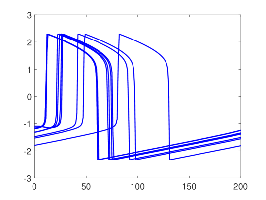
Figure 1: Reference solution for the $x$ component of the FN system, cells 1-5 and 50-55.

In Figure 2, the error and CPU ratios of standard ESDIRK method versus their economical variants are displayed, highlighting the superior performance of the proposed methods. In particular, it can be observed that the reformulation of the systems for the economical solvers allows in general to obtain a more effective error estimation, as well as to reduce the computational effort. A more detailed comparison of the error behaviour of different methods is shown in Figure 3, where we display the absolute errors for the $x$ component of the first cell in the network.

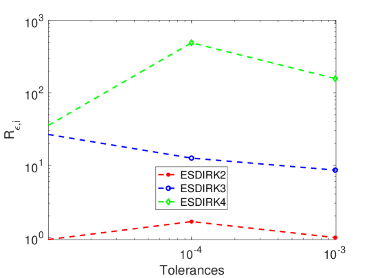
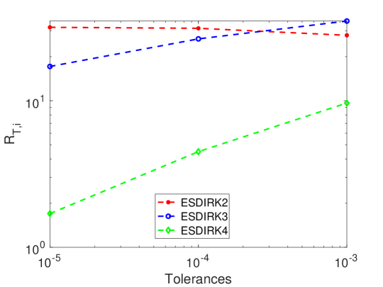
Figure 2: Errors (above) and CPU time (below) ratios with respect to different tolerances.

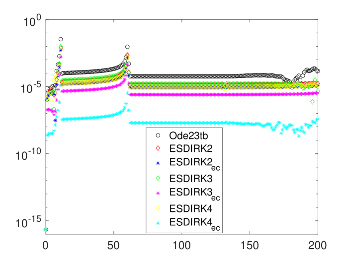
Figure 3: Time evolution of absolute error for $x$ component of the first cell in the network.

In the second test we have considered the non adaptive implementations and analyzed the dependency of the error on the size of the time step. Thus, we have taken all the parameters as in the previous test, and we have set the number of integration steps $M=100,200,400,800$ and $1600$ (corresponding to time step size $h=2,1,0.5,0.25$ and $0.125,$ respectively). The results are reported in figures 4 and 5. As it can be observed, while the error decreases as the number of steps is increased, see Figure 5, the CPU ratios remain approximately of the same size, see Figure 4. Notice that in this case, since no error estimation is involved and the economical solvers are, indeed, solving exactly the same problem as their standard counterparts, no error reduction is observed in the economical solvers with respect to the standard ones (see Figure 5).

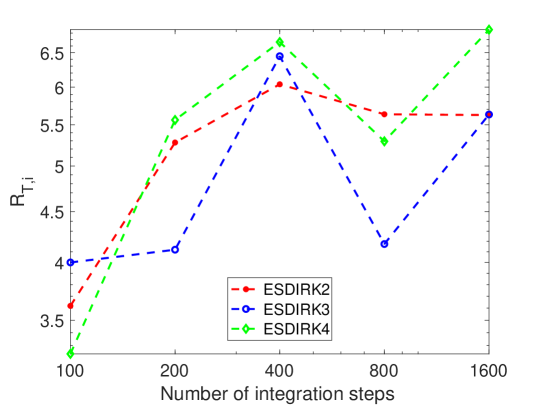
Figure 4: CPU time ratios with respect to number of integration steps.

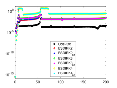
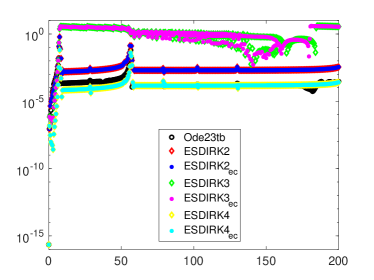
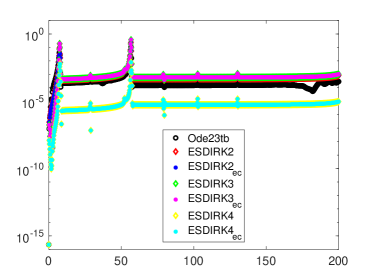
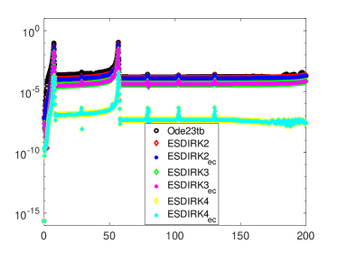
Figure 5: Time evolution of absolute error for $x$ component of the first cell in the network in cases $M=200$ (above, first case), 400 (above, second case), 800 (below, first case) and 1600 (below, second case).

6.2 Sensitivity to network size

In this second set of numerical experiments, we study how the performance of the proposed solvers depends on the network size. To do this, we consider again the FN network described in the first test of the previous Section, assuming $\tt atol=\tt rtol=10^{-4}$ and considering $N=10,10^{2},10^{3}$ cells. The results are shown in Figures 6 and 7. In particular, for the error ratios (first panel) we observe that the higher the order of the method, the better is the performance. This situation is reversed for the corresponding CPU ratios (second panel). In Figure 7 we represent the product of the ratios, and we observe that, overall, economical versions of the solvers are more efficient than the standard ones, and that again the higher the order of the method, the better is the performance.

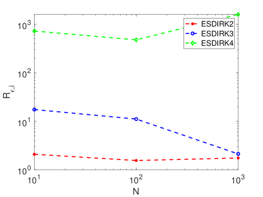
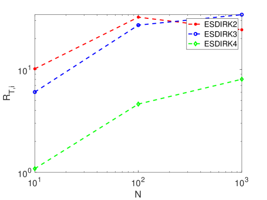
Figure 6: Error ratios (above) and CPU time ratios (below) as a function of network size $N$.

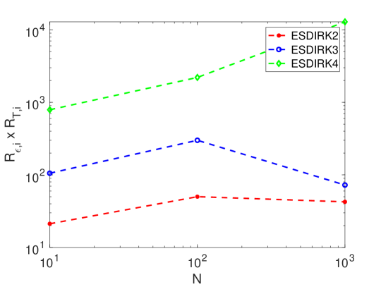
Figure 7: Product of error and CPU time ratios as a function of network size $N$.

6.3 Tests with different coupling matrices and timescales

In this third set of numerical experiments, we study how the performance depends on the sparsity of the coupling matrix and on the timescale separation. To do this, we consider now the HR network with $N=10^{3}$ cells and $\tt atol=\tt rtol=10^{-4}$. The initial conditions have been selected in each cell as $[x_{0},y_{0},z_{0}]=[-1.48+\delta,-10.06+\delta,1.84+\delta],$ where $\delta$ denotes a random variable with uniform distribution on $(-0.01,0.01),$ in order to start the simulation in a neighbourhood of the system attractor. In the first test, we have selected $\varepsilon=0.01$ and we have considered coupling matrices with the structure represented in Figure 8. Note that the plots actually show the case $N=10$ instead of $N=10^{3}$ for the sake of clarity.

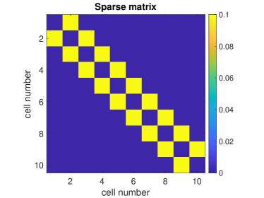
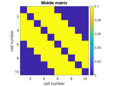
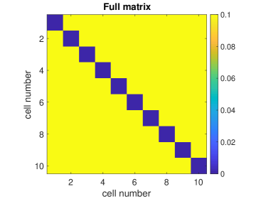
Figure 8: Structure of different coupling matrices for a network of $N=10$ cells.

Figure 9 shows the time evolution of the first component of cells 1-5 and 501-505 for the reference solution in the case of the sparse coupling matrix, displaying an early synchronization peak.

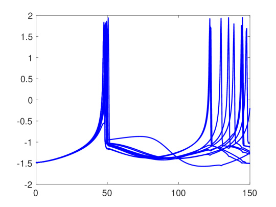
Figure 9: First component of cells 1-5 and 501-505 for the reference solution.

We report the error behaviour of different methods in Figure 10, where we display the absolute errors for the first component of the first cell in the network.

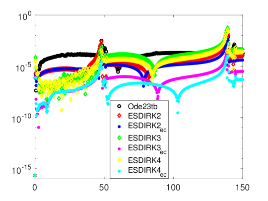
Figure 10: Time evolution of absolute error for first component.

Now, let us consider the three types of coupling matrices considered. The obtained results are shown in Figure 11.

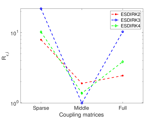
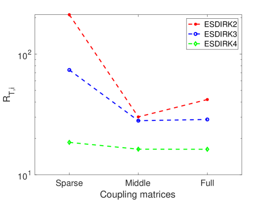
Figure 11: Errors (above) and CPU time (below) ratios with respect to different coupling matrices.

We observe in Figure 11 (second panel) that the less sparse is the matrix, the better is the performance of the economic versions of the methods with respect to the standard ones. However, regarding the error ratios, we do not observe such enhancement (see Figure 11, first panel).

In the second test, we have considered the sparse lattice matrix in case of $N=10$ cells (see first case in Figure 8) and we have selected timescale separation parameter values of $\varepsilon=0.001,0.005,0.01$ and $0.05$. We represent the results in Figure 12. In the first panel, we observe that for the intermediate $\varepsilon$ values, the higher the order of the method, the better is the performance with respect to the error ratios. In the right panel, we see that for $\varepsilon<10^{-2}$ the time ratios remain almost constant, which entails that the increasing stiffness of the problems does not affect the efficiency of the proposed methods.

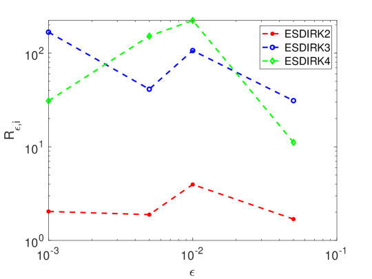
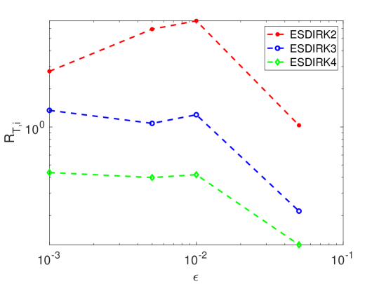
Figure 12: Errors (above) and CPU time (below) ratios with respect to timescale separation $\varepsilon$.

6.4 Test with a realistic network configuration

We consider here the ICC model on the type of network already studied in [1]. The network is composed of two different clusters, with the cells connected in-phase within each cluster and anti-phase between them. This configuration appears, for instance, in the motoneurons of the embrionic spinal cord of the zebrafish, see e.g. the discussion in [13]. The values chosen for the model parameters are the same as in the third example of Section 4.3 of [1], assuming that the first cluster is homogeneous and the second heterogeneous. In this case, only the third and fourth order economical solvers were considered and compared to the MATLAB solvers $\tt ode45$ and $\tt ode15s,$ used with the same value of the tolerance parameters $\tt atol=\tt rtol=10^{-6}$. In Figure 13, we report the time evolution of the $x$ variable in the first cell of the second cluster and of the absolute errors on the same variable for different solvers. It can be observed that, with the same tolerance, the economical ESDIRK solvers achieve superior accuracy with respect to the reference MATLAB solvers, even though due to lack of code optimization the required CPU time for the our implementation is more than one order of magnitude larger than that of the MATLAB solvers.

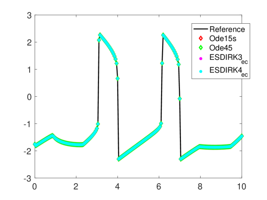
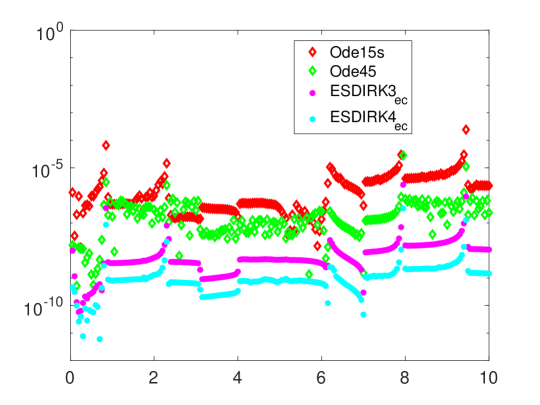
Figure 13: Time evolution of the $x$ variable in the first cell of the second cluster (above) and absolute errors for the same variable for different solvers (below).

7 Conclusions and future work

We have outlined a general method to build efficient, specific versions of standard implicit ODE solvers tailored for the simulation of neural networks. The specific versions of the ODE solvers proposed here allow to achieve a significant increase in the efficiency of network simulations, by reducing the size of the algebraic system being solved at each time step. This development is inspired by very successful semi-implicit approaches in computational fluid dynamics and structural mechanics.

While we have focused here specifically on Explicit first step, Diagonally Implicit Runge Kutta methods (ESDIRK), similar simplifications can be applied to any implicit ODE solver. In order to demonstrate the capabilities of the proposed methods, we have considered networks based on three different slow-fast single cells models, including the classical FitzHugh-Nagumo (FN) model, the Intracellular Calcium Concentration (ICC) model and the Hindmarsh-Rose (HR) system model. The numerical results obtained in a range of simulations of systems with different size and topology demonstrate the potential of the proposed method to increase substantially the efficiency of numerical simulations of neural networks.

In future developments, we plan more extensive applications of the proposed approach to the study of large scale neural networks of biological interest and to further improve the efficiency by developing self-adjusting multirate extensions of these numerical methods along the lines of [5].

References

- [1] A. Bandera, S. Fernández-García, M. Gómez-Mármol, and A. Vidal. A multiple timescale network model of intracellular calcium concentrations in coupled neurons: Insights from rom simulations. Mathematical Modelling of Natural Phenomena, 17:1–26, 2022.
- [2] R.E. Bank, W.M. Coughran, W. Fichtner, E.H. Grosse, D.J. Rose, and R.K. Smith. Transient Simulation of Silicon Devices and Circuits. IEEE Transactions on Electron Devices, 32:1992–2007, 1985.
- [3] E. Benoit, J.L. Callot, F. Diener, and M. Diener. Chasse au canard. Collectanea Mathematica, pages 37–76, 1981.
- [4] L. Bonaventura. A semi-implicit, semi-Lagrangian scheme using the height coordinate for a nonhydrostatic and fully elastic model of atmospheric flows. Journal of Computational Physics, 158:186–213, 2000.
- [5] L. Bonaventura, F. Casella, L. Delpopolo Carciopolo, and A. Ranade. A self adjusting multirate algorithm for robust time discretization of partial differential equations. Computers & Mathematics with Applications, 79:2086–2098, 2020.
- [6] L. Bonaventura and M. Gómez Marmol. The TR-BDF2 method for second order problems in structural mechanics. Computers & Mathematics with Applications, 92:13–26, 2021.
- [7] S. A. Campbell and M. Waite. Multistability in coupled FitzHugh–Nagumo oscillators. Nonlinear Analysis: Theory, Methods & Applications, 47(2):1093–1104, 2001.
- [8] V. Casulli. Semi-implicit finite difference methods for the two dimensional shallow water equations. Journal of Computational Physics, 86:56–74, 1990.
- [9] R.T. Q. Chen, Y. Rubanova, J. Bettencourt, and D.K. Duvenaud. Neural Ordinary Differential Equations. Advances in neural information processing systems, 31, 2018.
- [10] M. Desroches, J. Guckenheimer, B. Krauskopf, C. Kuehn, H.M. Osinga, and M. Wechselberger. Mixed-mode oscillations with multiple time scales. SIAM Rev., 54(2):211–288, 2012.
- [11] B. Ermentrout, M. Pascal, and B. Gutkin. The effects of spike frequency adaptation and negative feedback on the synchronization of neural oscillators. Neural Computation, 13:1285–1310, 2001.
- [12] A. S. Etémé, C. B. Tabi, and A. Mohamadou. Long-range patterns in Hindmarsh-Rose networks. Communications in Nonlinear Science and Numerical Simulation, 43:211–219, 2017.
- [13] F. V. Fallani, M. Corazzol, J. R. Sternberg, C. Wyart, and M. Chavez. Hierarchy of neural organization in the embryonic spinal cord: Granger-causality graph analysis of in vivo calcium imaging data. IEEE Transactions on Neural Systems and Rehabilitation Engineering, 23(3):333–341, 2015.
- [14] S. Fernández-García and A. Vidal. Symmetric coupling of multiple timescale systems with mixed-mode oscillations and synchronization. Physica D: Nonlinear Phenomena, 401:132129, 2020.
- [15] R. FitzHugh. Impulses and physiological states in theoretical models of nerve membrane. Biophysical Journal, 1(6):445–466, 1961.
- [16] E. Hairer, S.P. Nørsett, and G. Wanner. Solving Ordinary Differential Equations I: Nonstiff Problems. Springer-Verlag, Berlin Heidelberg, 3rd corr. edition, 2008.
- [17] J. L. Hindmarsh and R. M. Rose. A model of neural bursting using three coupled first order differential equations. Proceedings of the Royal Society of London B, 221(1222):87–102, 1984.
- [18] A.L. Hodgkin and A.F. Huxley. A quantitative description of membrane current and its application to conduction and excitation in nerve. The Journal of Physiology, 117:500–544, 1952.
- [19] M.E. Hosea and L.F. Shampine. Analysis and implementation of TR-BDF2. Applied Numerical Mathematics, 20:21–37, 1996.
- [20] M. M. Ibrahim and I. H. Jung. Complex synchronization of a ring-structured network of FitzHugh-Nagumo neurons with single-and dual-state gap junctions under ionic gates and external electrical disturbance. IEEE Access, 7:57894–57906, 2019.
- [21] E. M. Izhikevich. Neural excitability, bursting and spiking. Int. J. Bifurcation Chaos, 10(6):1171–1266, 2000.
- [22] H. Jaeger, M. Lukoševičius, D. Popovici, and U. Siewert. Optimization and applications of echo state networks with leaky-integrator neurons. Neural Networks, 20:335–352, 2007.
- [23] C. A. Kennedy and M.H. Carpenter. Diagonally implicit Runge-Kutta methods for Ordinary Differential Equations, a review. Technical Report TM-2016-219173, NASA, 2016.
- [24] C. A. Kennedy and M.H. Carpenter. Diagonally implicit Runge–Kutta methods for stiff ODEs. Applied Numerical Mathematics, 146:221–244, 2019.
- [25] M. Krupa, A. Vidal, and F. Clément. A network model of the periodic synchronization process in the dynamics of calcium concentration in GnRH neurons. Journal of Mathematical Neuroscience, 3:1–24, 2013.
- [26] J.D. Lambert. Numerical methods for ordinary differential systems: the initial value problem. Wiley, 1991.
- [27] W. Maass. Liquid State Machines: motivation, theory, and applications, pages 275–296. World Scientific, 2011.
- [28] W. Maass, T. Natschläger, and H. Markram. Real-time computing without stable states: A new framework for neural computation based on perturbations. Neural Computing, 14:2531–2560, 2002.
- [29] J. Nagumo, S. Arimoto, and S. Yoshizawa. An active pulse transmission line simulating nerve axon. Proceedings of the IRE, 50(10):2061–2070, 1962.
- [30] J. Rinzel. A formal classification of bursting mechanisms in excitable systems. Mathematical Topics in Population Biology, Morphogenesis, and Neurosciences, 71, 1987.
- [31] B.I. Yildiz, H. Jaeger, and S.J. Kiebel. Re-visiting the echo state property. Neural Networks, 35:1–9, 2012.
- [32] Z. Yong, Z. Su-Hua, Z. Tong-Jun, A. Hai-Long, Z. Zhen-Dong, H. Ying-Rong, L. Hui, and Z. Yu-Hong. The synchronization of FitzHugh-Nagumo neuron network coupled by gap junction. Chinese Physics B, 17:2297–07, 2008.