Clean self-supervised MRI reconstruction from noisy, sub-sampled training data with Robust SSDU

Abstract

Most existing methods for Magnetic Resonance Imaging (MRI) reconstruction with deep learning use fully supervised training, which assumes that a high signal-to-noise ratio (SNR), fully sampled dataset is available for training. In many circumstances, however, such a dataset is highly impractical or even technically infeasible to acquire. Recently, a number of self-supervised methods for MR reconstruction have been proposed, which use sub-sampled data only. However, the majority of such methods, such as Self-Supervised Learning via Data Undersampling (SSDU), are susceptible to reconstruction errors arising from noise in the measured data. In response, we propose Robust SSDU, which provably recovers clean images from noisy, sub-sampled training data by simultaneously estimating missing k-space samples and denoising the available samples. Robust SSDU trains the reconstruction network to map from a further noisy and sub-sampled version of the data to the original, singly noisy and sub-sampled data, and applies an additive Noisier2Noise correction term at inference. We also present a related method, Noiser2Full, that recovers clean images when noisy, fully sampled data is available for training. Both proposed methods are applicable to any network architecture, straight-forward to implement and have similar computational cost to standard training. We evaluate our methods on the multi-coil fastMRI brain dataset with a novel denoising-specific architecture and find that it performs competitively with a benchmark trained on clean, fully sampled data.

I Introduction

Magnetic Resonance Imaging (MRI) has excellent soft tissue contrast and is the gold standard modality for a number of clinical applications. A hindrance of MRI, however, is its lengthy acquisition time, which is especially challenging when high spatio-temporal resolution is required, such as for dynamic imaging [1]. To address this, there has been substantial research attention on methods that reduce the acquisition time without significantly sacrificing the diagnostic quality [2, 3, 4]. In MRI, measurements are acquired in the Fourier representation of the image, referred to in the MRI literature as “k-space”. Since the acquisition time is roughly proportional to the number of k-space samples, acquisitions can be accelerated by sub-sampling. A reconstruction algorithm is then employed to estimate the image from the sub-sampled data.

In recent years, reconstructing sub-sampled MRI data with neural networks has emerged as the state-of-the-art [5, 6, 7]. The majority of existing methods assume that a fully sampled dataset is available for fully-supervised training. However, for many applications, no such dataset is available, and may be difficult or even infeasible to acquire in practice [8, 9, 10]. In response, there has been a number of self-supervised methods proposed, which train on sub-sampled data only [11, 12, 13, 14].

Most existing training methods assume that the measurement noise is small and do not denoise sampled data. Section III shows that without denoising the reconstruction quality degrades when the measurement noise increases. This is a particular concern for low SNR applications, such as for the increasing interest in low-cost, low-field scanners [15, 16, 17].

In response, this paper presents a modification of Self-Supervised Learning via Data Undersampling (SSDU) [13] that also removes measurement noise, building on the present authors’ recent work [18] on the connection between SSDU and the multiplicative version of the self-supervised denoising method Noisier2Noise [19]. Our method, which we term “Robust SSDU”, combines SSDU with additive Noisier2Noise for simultaneous self-supervised reconstruction and denoising. In brief, Robust SSDU trains a network to map from a further sub-sampled and further noisy version of the training data to the original sub-sampled, noisy data. Then, at inference, a correction is applied to the network that ensures that the clean (i.e. noise-free) image is recovered in expectation. We find that Robust SSDU performs competitively with a best-case benchmark where the network is trained on clean, fully sampled data, despite training on noisy, sub-sampled data only. We also propose a related method that recovers clean images for the simpler task of when fully sampled, noisy data is available for training, which we term “Noisier2Full”. Both Noisier2Full and Robust SSDU are fully mathematically justified and have minimal additional computational expense compared to standard training.

The existing method most similar to Robust SSDU is Noise2Recon-Self-Supervised (Noise2Recon-SS) [20]. We find that Robust SSDU offers substantial image quality improvements over Noise2Recon-SS in practice and a two-fold reduction in computational cost at training: see Section V.

II Theory: background

This section reviews key works from the literature that form the bases of the methods proposed in this paper.

II-A Self-supervised denoising with Noisier2Noise

Denoising with deep learning concerns the task of recovering a clean $q$-dimensional vector from noisy measurements

$$y_{t}=y_{0,t}+n_{t},$$

where $n_{t}$ is noise and $t$ indexes the training set. In MRI, noise in k-space is modeled as complex Gaussian with zero mean, $n_{t}\backsim\mathcal{CN}(0,\Sigma^{2}_{n})$, where $\Sigma^{2}_{n}$ is a covariance matrix that can be estimated, for instance, with an empty pre-scan [21]. In this paper, the noise is modeled as white, $\Sigma^{2}_{n}=\sigma_{n}^{2}\mathds{1}$. Although multi-coil MR data has non-trivial $\Sigma^{2}_{n}$ in general, we note that the noise can be whitened by left-multiplying $y_{t}$ with $\Sigma^{-1}_{n}$. We refer

Self-supervised denoising concerns the task of training a network to remove noise when the training data is itself noisy [22, 23, 24, 25]. This paper focuses on additive Noisier2Noise [19] because we find that it offers a natural way to extend image reconstruction to low SNR data: see Section III.

Noisier2Noise’s training procedure consists of corrupting the noisy training data with further noise, and training a network to recover the singly noisy image from the noisier image. Concretely, further noise is introduced to $y_{t}$,

$$\widetilde{y}_{t}=y_{t}+\widetilde{n}_{t}=y_{0,t}+n_{t}+\widetilde{n}_{t},$$ (1)

where $\widetilde{n}_{t}\backsim\mathcal{CN}(0,\alpha^{2}\sigma^{2}_{n}\mathds{1})$ for a constant $\alpha$. Then, a network $f_{\theta}$ with parameters $\theta$ is trained to minimize

$$\hat{\theta}=\underset{\theta}{\arg\min}\sum_{t}\|f_{\theta}(\widetilde{y}_{t})-y_{t}\|^{2}_{2}.$$ (2)

The following result states that a simple transform of the trained network yields the clean $y_{0,t}$ in expectation.

Result 1.

Consider the random variables $Y=Y_{0}+N$ and $\widetilde{Y}=Y+\widetilde{N}$, where $N$ and $\widetilde{N}$ are zero-mean Gaussian distributed with variances $\sigma_{n}^{2}$ and $\alpha^{2}\sigma_{n}^{2}$ respectively. Minimizing

$$\theta^{*}=\underset{\theta}{\arg\min}\hskip 2.84544pt\mathds{E}[\|f_{\theta}(\widetilde{Y})-Y\|^{2}_{2}|\widetilde{Y}]$$ (3)

yields a network that satisfies

$$\mathds{E}[Y_{0}|\widetilde{Y}]=\frac{(1+\alpha^{2})f_{\theta^{*}}(\widetilde{Y})-\widetilde{Y}}{\alpha^{2}}.$$

Proof.

See Section 3.3 of [19]. ∎

Here, (3) can be thought of as (2) in the limit of an infinite number of samples, and $\hat{\theta}$ as a finite sample approximation of $\theta^{*}$. Result 1 states that the clean image can be estimated in conditional expectation by employing a correction term based on $\alpha$ at inference. In practice,

$$\hat{y}_{s}=\frac{(1+\alpha^{2})f_{\hat{\theta}}(\widetilde{y}_{s})-\widetilde{y}_{s}}{\alpha^{2}}$$ (4)

is used, where $s$ indexes the test set.

II-B Self-supervised reconstruction with SSDU

This section focuses on the case where the data consists of noise-free, sub-sampled data

$$y_{t}=M_{\Omega_{t}}y_{0,t}.$$

Here, $M_{\Omega_{t}}$ is a sampling mask, a diagonal matrix with $j$th diagonal 1 when $j\in\Omega_{t}$ and 0 otherwise for sampling set $\Omega_{t}\subseteq\{1,2,\ldots,q\}$.

Self-supervised reconstruction consists of training a network to recover images when only sub-sampled data is available for training [26]. This work focuses on the popular method SSDU [13], which was theoretically justified in [18] via the multiplicative noise version of Noiser2Noise [19]. In this framework, analogous to the further noise used in (1), the data is further sub-sampled by applying a second mask with sampling set $\Lambda_{t}\subseteq\{1,2,\ldots,q\}$ to $y_{t}$,

$$\widetilde{y}_{t}=M_{\Lambda_{t}}y_{t}=M_{\Lambda_{t}\cap\Omega_{t}}y_{0,t},$$ (5)

where $M_{\Lambda_{t}\cap\Omega_{t}}=M_{\Lambda_{t}}M_{\Omega_{t}}$. Training consists of minimizing a loss function on indices in $\Omega_{t}\setminus\Lambda_{t}$, such as

$$\hat{\theta}=\underset{\theta}{\arg\min}\sum_{t}\|M_{\Omega_{t}\setminus\Lambda_{t}}(f_{\theta}(\widetilde{y}_{t})-y_{t})\|^{2}_{2},$$ (6)

where $M_{\Omega_{t}\setminus\Lambda_{t}}=(\mathds{1}-M_{\Lambda_{t}})M_{\Omega_{t}}$. Although for theoretical ease we state SSDU with an $\ell_{2}$ loss here, it is known that other losses are possible [13].

Let $p_{j}=\mathds{P}[j\in\Omega]$ and $\widetilde{p}_{j}=\mathds{P}[j\in\Lambda]$. Assuming that

$$p_{j} >0\hskip 5.69046pt\forall\hskip 2.84544ptj,$$ (7)

$$\widetilde{p}_{j}<1 \hskip 5.69046pt\forall\hskip 2.84544pt\{j:p_{j}<1\},$$ (8)

the following result from [18] proves that SSDU recovers the clean image in expectation.

Result 2.

Consider the random variables $Y=M_{\Omega}Y_{0}$ and $\widetilde{Y}=M_{\Lambda}Y$, where $N$ and $\widetilde{N}$ are zero-mean Gaussian distributed with variances $\sigma_{n}^{2}$ and $\alpha^{2}\sigma_{n}^{2}$ respectively. When (7) and (8) hold, minimizing

$$\theta^{*}=\underset{\theta}{\arg\min}\sum_{t}\|M_{\Omega\setminus\Lambda}(f_{\theta}(\widetilde{Y})-Y)\|^{2}_{2}$$ (9)

yields a network with parameters that satisfies

$$M_{(\Lambda\cap\Omega)^{c}}\mathds{E}[Y_{0}|\widetilde{Y}]=M_{(\Lambda\cap\Omega)^{c}}f_{\theta^{*}}(\widetilde{Y}).$$ (10)

Proof.

See Appendix B of [18]. ∎

Result 2 states that the network correctly estimates $Y_{0}$ in conditional expectation for indices not in $\Lambda\cap\Omega$. To estimate everywhere in k-space one can overwrite sampled indices or use a data consistent architecture: see [18] for details.

III Theory: proposed methods

The reminder of this paper considers the task of training a network to recover images from noisy, sub-sampled data

$$y_{s}=M_{\Omega_{s}}(y_{0,s}+n_{s}).$$

It has been stated that when a network reconstructs noisy MRI data with a standard training method, there is a denoising effect [16]. In the following, we motivate the need for methods that explicitly remove noise by showing that the apparent noise removal is in fact a “pseudo-denoising” effect due to the correct estimation in expectation of indices in $\Omega^{c}$.

Consider the standard approach of training a network to map from noisy, sub-sampled $y_{t}$ to noisy, fully sampled $y_{0,t}+n_{t}$. In terms of random variables, training consists of minimizing

$$\theta^{*}=\underset{\theta}{\arg\min}\hskip 2.84544pt\mathds{E}[\|f_{\theta}(Y)-(Y_{0}+N)\|^{2}_{2}|Y],$$

which gives a network that satisfies

$$f_{\theta^{*}}(Y)=\mathds{E}[Y_{0}+N|Y].$$ (11)

It is instructive to examine how $\mathds{E}[Y_{0}+N|Y]$ depends on the sampling mask $\Omega$. Firstly, for $j\notin\Omega$,

$$\mathds{E}[Y_{0,j}+N_{j}|Y,j\notin\Omega] =\mathds{E}[Y_{0,j}|Y]+\mathds{E}[N_{j}]$$

$$=\mathds{E}[Y_{0,j}|Y],$$ (12)

where we have used the independence of $N_{j}$ from $Y$ when $j\notin\Omega$ and $\mathds{E}[N_{j}]=0$ by assumption. For the alternative $j\in\Omega$,

$$\mathds{E}[Y_{0,j}+N_{j}|Y,j\in\Omega]=\mathds{E}[Y_{j}|Y]=Y_{j}$$

where $Y_{0,j}+N_{j}=Y_{j}$ for $j\in\Omega$ has been used. The trained network therefore satisfies

$$f_{\theta^{*}}(Y)=\mathds{E}[Y_{0}+N|Y]=M_{\Omega^{c}}\mathds{E}[Y_{0}|Y]+M_{\Omega}Y.$$

Therefore the network targets the noise-free $Y_{0,j}$ in regions in $\Omega^{c}$ but recovers the noisy $Y$ otherwise. As there is less total measurement noise present than $Y_{0}+N$, this gives the impression of noise removal, however, we emphasize that the network does not remove the noise in $Y$; hence the use of the term “pseudo-denoising”.

We refer to this method described in this section as “Noise2Full” throughout this paper. In the following we propose methods that explicitly recover $Y_{0}$ in conditional expectation from noisy, sub-sampled inputs in two cases: A) the training data is noisy and fully sampled; B) the training data is noisy and sub-sampled. For tasks A and B we propose “Noisier2Full” and “Robust SSDU” respectively.

III-A Noisier2Full for fully sampled, noisy training data

This section proposes Noisier2Full, which extends additive Noisier2Noise to reconstruction tasks for noisy, fully sampled training data. Based on (1), we propose corrupting the measurements $y_{t}$ with further noise on the sampled indices,

$$\widetilde{y}_{t}=y_{t}+M_{\Omega_{t}}\widetilde{n}_{t}.$$

Then we minimize the loss between $\widetilde{y}_{t}$ and the noisy, fully sampled training data $y_{0,t}+n_{t}$. In terms of random variables,

$$\theta^{*}=\underset{\theta}{\arg\min}\hskip 2.84544pt\mathds{E}[\|f_{\theta}(\widetilde{Y})-(Y_{0}+N)\|^{2}_{2}|\widetilde{Y}].$$ (13)

Minimizing the $\ell_{2}$ norm gives a network that satisfies

$$f_{\theta^{*}}(\widetilde{Y})=\mathds{E}[Y_{0}+N|\widetilde{Y}],$$

which is recognizable as (11) with $Y$ replaced by $\widetilde{Y}$. Similarly to (12), $N_{j}$ is independent of $\widetilde{Y}$ when $j\notin\Omega$, so the ground truth is estimated in such regions:

$$\mathds{E}[Y_{0,j}|\widetilde{Y},j\notin\Omega]=\mathds{E}[Y_{0,j}|\widetilde{Y}].$$

However, crucially, the expectation is conditional on $\widetilde{Y}$, not $Y$, so the additive Noisier2Noise correction stated in Result 1 is applicable when $j\in\Omega$:

$$\mathds{E}[Y_{0,j}|\widetilde{Y},j\in\Omega]=\frac{(1+\alpha^{2})f_{\theta^{*}}(\widetilde{Y})_{j}-\widetilde{Y}_{j}}{\alpha^{2}}$$

Therefore $Y_{0}$ can be estimated with

$$\mathds{E}[Y_{0}|\widetilde{Y}]=M_{\Omega}\left(\frac{(1+\alpha^{2})f_{\theta^{*}}(\widetilde{Y})-\widetilde{Y}}{\alpha^{2}}\right)+M_{\Omega^{c}}f_{\theta^{*}}(\widetilde{Y}).$$ (14)

In summary, Noisier2Full recovers $Y_{0}$ in conditional expectation by introducing further noise to the sampled indices during training, and correcting those indices at inference via additive Noisier2Noise. In the subsequent section, we show how this approach can extended to the more challenging case where the training data is also sub-sampled.

III-B Robust SSDU for sub-sampled, noisy training data

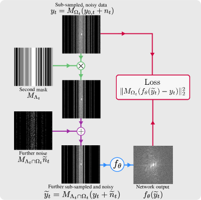
Figure 1: The proposed self-supervised reconstruction and denoising method Robust SSDU, which extends the training procedure illustrated in Fig. 1 of [18] to low SNR data. The sub-sampled, noisy training data $y_{t}$ is further sub-sampled by a mask $M_{\Lambda_{t}}$ and corrupted by further noise $\widetilde{n}_{t}$, yielding $\widetilde{y}_{t}$. The loss is computed between $y_{t}$ and $f_{\theta}(\widetilde{y}_{t})$ on $\Omega_{t}$.

This section proposes Robust SSDU, which recovers clean images in conditional expectation when the training data is both noisy and sub-sampled. Robust SSDU combines the approaches from Sections II-A and II-B to simultaneously reconstruct and denoise the data: see Fig. 1 for a schematic. We propose combining (1) and (5) to form a vector that is further sub-sampled and additionally noisy,

$$\widetilde{y}_{t}=M_{\Lambda_{t}\cap\Omega_{t}}(y_{t}+\widetilde{n}_{t}).$$

Recall that SSDU employs $M_{\Omega\setminus\Lambda}$ in the loss, which yields a network that estimates indices in $(\Lambda\cap\Omega)^{c}$: see Result 2. For Robust SSDU we replace $M_{\Omega\setminus\Lambda}$ with $M_{\Omega}$, so that the loss is

$$\hat{\theta}=\underset{\theta}{\arg\min}\sum_{t}\|M_{\Omega_{t}}(f_{\theta}(\widetilde{y}_{t})-y_{t})\|^{2}_{2}.$$

In the following we show that this change leads to estimation everywhere in k-space, not just indices in $(\Lambda\cap\Omega)^{c}$.

Claim 1.

Consider the random variables $Y=M_{\Omega}(Y_{0}+N)$ and $\widetilde{Y}=M_{\Lambda\cap\Omega}(Y+\widetilde{N})$, where $N$ and $\widetilde{N}$ are zero-mean Gaussian distributed with variances $\sigma_{n}^{2}$ and $\alpha^{2}\sigma_{n}^{2}$ respectively. When (7) and (8) hold, minimizing

$$\theta^{*}=\underset{\theta}{\arg\min}\hskip 2.84544pt\mathds{E}[\|M_{\Omega}(f_{\theta}(\widetilde{Y})-Y)\|_{2}^{2}|\widetilde{Y}].$$ (15)

yields a network with parameters that satisfies

$$f_{\theta^{*}}(\widetilde{Y})=\mathds{E}[Y_{0}+N|\widetilde{Y}].$$

Proof.

See appendix VII-A. ∎

At inference, we can use a similar approach to Section III-A, applying the additive Noisier2Noise correction on indices sampled in $\widetilde{Y}$. Since the indices sampled in $\widetilde{Y}$ are $\Lambda\cap\Omega$, the clean image $Y_{0}$ is estimable with

$$\mathds{E}[Y_{0}|\widetilde{Y}]=M_{\Lambda\cap\Omega}\left(\frac{(1+\alpha^{2})f_{\theta^{*}}(\widetilde{Y})-\widetilde{Y}}{\alpha^{2}}\right)\\ +M_{(\Lambda\cap\Omega)^{c}}f_{\theta^{*}}(\widetilde{Y}).$$ (16)

Roughly speaking, Robust SSDU can be thought of as a generalization of Noisier2Full to sub-sampled training data. Specifically, Robust SSDU is mathematically equivalent to Noisier2Full when $\Omega=\{1,2,\ldots,q\}$ and there is the change of notation $\Lambda\rightarrow\Omega$. More broadly, Robust SSDU can be interpreted as the simultaneous application of additive and multiplicative Noisier2Noise [19, 18].

III-C Weighted variants of Noisier2Full and Robust SSDU

For Noisier2Full and Robust SSDU, the task at training and inference is not identical: at training the network maps from $\widetilde{Y}$ to $Y_{0}+N$ or $M_{\Omega}(Y_{0}+N)$, while at inference it maps from $\widetilde{Y}$ to $Y_{0}$ via the $\alpha$-based correction term. Taking a similar approach to [27, 28], this section describes how this can be compensated for by modifying the loss function in such a way that its gradient equals the gradient of the target loss in conditional expectation.

Claim 2.

Consider the random variables $Y=M_{\Omega}(Y_{0}+N)$ and $\widetilde{Y}=Y+M_{\Omega}\widetilde{N}$, where $N$ and $\widetilde{N}$ are zero-mean Gaussian distributed with variances $\sigma_{n}^{2}$ and $\alpha^{2}\sigma_{n}^{2}$ respectively. Define

$$\hat{Y}_{Nr2F}=M_{\Omega}\left(\frac{(1+\alpha^{2})f_{\theta}(\widetilde{Y})-\widetilde{Y}}{\alpha^{2}}\right)+M_{\Omega^{c}}f_{\theta}(\widetilde{Y})$$

where $f_{\theta}$ is an arbitrary function. Then

$$\nabla_{\theta}\mathds{E}\left[\left\|\hat{Y}_{Nr2F}-Y_{0}\right\|^{2}_{2}|\widetilde{Y}\right]\\ =\nabla_{\theta}\mathds{E}\left[\left\|\left(\frac{1+\alpha^{2}}{\alpha^{2}}M_{\Omega}+M_{\Omega^{c}}\right)(f_{\theta}(\widetilde{Y})-Y_{0}-N)\right\|^{2}_{2}|\widetilde{Y}\right].$$ (17)

Proof.

See appendix VII-B. ∎

We therefore suggest replacing the Noisier2Full loss stated in (13) with the right-hand-side of (17), which increases the weight of the indices in $\Omega$. Intuitively, it uses the ratio of noise removed at training, which has variance $\mathrm{Var}(\widetilde{N})=\alpha^{2}\sigma_{n}^{2}$, and the noise removed at inference, which has variance $\mathrm{Var}(N+\widetilde{N})=(1+\alpha^{2})\sigma_{n}^{2}$, to compensate for the difference between the task at training and inference. The following result concerns the analogous expression for Robust SSDU.

Claim 3.

Consider the random variables $Y=M_{\Omega}(Y_{0}+N)$ and $\widetilde{Y}=M_{\Lambda\cap\Omega}(Y+\widetilde{N})$, where $N$ and $\widetilde{N}$ are zero-mean Gaussian distributed with variances $\sigma_{n}^{2}$ and $\alpha^{2}\sigma_{n}^{2}$ respectively. Define

$$\hat{Y}_{RSSDU}=M_{\Lambda\cap\Omega}\left(\frac{(1+\alpha^{2})f_{\theta}(\widetilde{Y})-\widetilde{Y}}{\alpha^{2}}\right)+M_{(\Lambda\cap\Omega)^{c}}f_{\theta^{*}}(\widetilde{Y})$$

where $f_{\theta}$ is an arbitrary function. Then

$$\mathds{E}\left[\left\|\hat{Y}_{RSSDU}-Y_{0}\right\|^{2}_{2}|\widetilde{Y}\right]\\ =\nabla_{\theta}\mathds{E}\left[\left\|\left(\frac{1+\alpha^{2}}{\alpha^{2}}M_{\Lambda\cap\Omega}+\mathcal{P}^{\frac{1}{2}}M_{\Omega\setminus\Lambda}\right)(f_{\theta}(\widetilde{Y})-Y)\right\|^{2}_{2}|\widetilde{Y}\right]$$ (18)

where

$$\mathcal{P}=\mathds{E}[M_{\Omega\setminus\Lambda}]^{-1}\mathds{E}[M_{(\Lambda\cap\Omega)^{c}}].$$ (19)

Proof.

See appendix VII-C. ∎

The $M_{\Lambda\cap\Omega}$ coefficient has a similar role to the $M_{\Omega}$ coefficient in (17). The $M_{\Omega\setminus\Lambda}$ coefficient compensates for the variable density of $\Omega$ and $\Lambda$, and was first proposed in [18], where it was shown to improve the reconstruction quality and robustness to the distribution of $\Lambda$ for standard SSDU without denoising.

The weightings can be thought of as entry-wise modifications of the learning rate [18]. Neither weighting matrices change $\theta^{*}$, so the proofs of Noisier2Full and Robust SSDU from Sections III-A and III-B hold. Rather, the role of the weights is to improve the finite-sample case in practice, where $\theta^{*}$ is estimated with $\hat{\theta}$: see Section V for an empirical evaluation.

IV Materials and methods

IV-A Description of data

We used the multi-coil brain data from the publicly available fastMRI dataset [29]. We only used data that had 16 coils, so that the training, validation and test sets contained 2004, 320 and 224 slices respectively. The slices were normalized so that the cropped RSS estimate had maximum 1. Here, the cropped RSS is defined as $Z((\sum_{c}^{N_{c}}|F^{H}{y}_{c}|^{2})^{\frac{1}{2}})$, where the subscript $c$ refers to all entries on the $c$th coil, $F$ is the discrete Fourier transform, $N_{c}$ is the number of coils and $Z$ is an operator that crops to a central $320\times 320$ region. We retrospectively sub-sampled column-wise with the central 10 lines fully sampled and randomly drawn with polynomial density otherwise, with the probability density scaled to achieve a desired acceleration factor $R_{\Omega}=q/\sum_{j}p_{j}$. The data was treated as noise-free, and we generated white, complex Gaussian measurement noise with standard deviation $\sigma_{n}$ to simulate noisy conditions. An implementation of our method in PyTorch will be made available on GitHub.

IV-B Comment on the proposed methods in practice

The theoretical guarantees for Noisier2Full and Robust SSDU use the further noisy, possibly further sub-sampled $\widetilde{y}_{s}$ as the input to the network at inference. In practice, as suggested in the original Noisier2Noise [19] and SSDU [13] papers, we used $y_{s}$ as the input to the network at inference, so that the estimate

$$\hat{y}_{s}=M_{\Omega_{s}}\left(\frac{(1+\alpha^{2})f_{\hat{\theta}}(y_{s})-y_{s}}{\alpha^{2}}\right)+M_{\Omega_{s}^{c}}f_{\hat{\theta}}(y_{s})$$

is used in place of (14) and (16). Although this deviates from strict theory, and is not guaranteed to be correct in conditional expectation, we have found that it achieves better reconstruction performance in practice: see [19] and [18] for a detailed empirical evaluation. All subsequent results for the proposed methods use this estimate at inference.

IV-C Comparative training methods

For noise-free, fully sampled training data, fully supervised training can be employed. Although it is possible in principle to have higher SNR data at training than at inference by acquiring multiple averages [30], such datasets would require an extended acquisition time and are rare in practice. Nonetheless, training a network on this type of data via simulation is instructive as a best-case target. This method is referred to as the “best-case benchmark” throughout this paper.

For noisy, fully sampled training data, we employed three training methods: the proposed Noisier2Full and Weighted Noisier2Full and the standard approach Noise2Full, as described in Section III. We did not compare with Noise2Inverse [31] as it was designed for learned denoising but fixed reconstruction operators.

For the more challenging scenario where noisy, sub-sampled training data is available, we compared Robust SSDU and Weighted Robust SSDU with the original version of SSDU, which reconstructs sub-sampled data but does not denoise. We refer to this as “Standard SSDU”. We also compared with Noise2Recon-SS [20], which, like Robust SSDU, includes adding further noise to the sub-sampled data. However, Noise2Recon-SS has a number of key differences to the method proposed in this paper. With an $\ell_{2}$ k-space loss, training with Noise2Recon-SS consists of minimizing

$$\hat{\theta}=\underset{\theta}{\arg\min}\sum_{t}\|M_{\Omega_{t}\setminus\Lambda_{t}}(f_{\theta}(M_{\Lambda_{t}}y_{t})-y_{t})\|^{2}_{2}\\ +\lambda\|f_{\theta}(y_{t}+M_{\Omega_{t}}\widetilde{n}_{t})-f_{\theta}(M_{\Lambda_{t}}y_{t})\|^{2}_{2},$$

where $\lambda$ is a hand-selected weighting. We used $\lambda=1$ throughout. The $\ell_{2}$ loss in k-space was used so that it could be fairly compared to the other methods, but we note that [20] used image-domain losses. The first term is based on SSDU, and the second ensures that $f_{\theta}(y_{t}+M_{\Omega_{t}}\widetilde{n}_{t})$ and $f_{\theta}(M_{\Lambda_{t}}y_{t})$ yield similar outputs, so that the method is in a sense robust to $\widetilde{n}_{t}$. At inference, Noise2Recon-SS uses $\hat{y}_{s}=f_{\hat{\theta}}(y_{s})$; there is no correction term. We emphasize that, unlike the proposed Robust SSDU, there is no theoretical evidence that Noise2Recon-SS recovers the clean image in expectation.

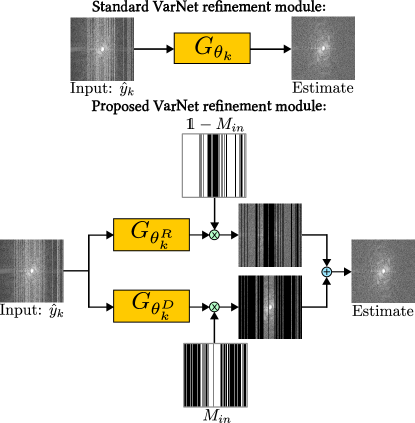
Figure 2: The refinement module for the proposed architecture Denoising VarNet, which trains two networks in parallel, removing noise and aliasing separately.

IV-D Network architecture and training details

All training methods considered in this paper are agnostic to the network architecture. We employed a network architecture based on the Variational Network (VarNet) [7, 32], which is available as part of the fastMRI package [29]. VarNet consists of a coil sensitivity map estimation module followed by a series of “cascades”. The k-space estimate at the $k$th cascade takes the form

$$\hat{y}_{k+1}=\hat{y}_{k}-\eta_{k}M_{in}(\hat{y}_{k}-y_{in})+G_{\theta_{k}}(\hat{y}_{k})$$

where $y_{in}$ and $M_{in}$ are the input k-space and sampling mask respectively and the $t$ or $s$ index has been dropped for legibility. We use the generic subscript $in$ here because the input is not the same for every method: for instance, fully-supervised and Noisier2Full have $M_{in}=M_{\Omega_{t}}$ and $M_{in}=M_{\Lambda_{t}\cap\Omega_{t}}$ respectively. Here, $\eta_{k}$ is a trainable parameter and $G_{\theta_{k}}(\hat{y}_{k})$ is a neural network with cascade-dependent parameters $\theta_{k}$, referred to as a “refinement module”, which was an image-domain U-net [33] in [7, 32].

VarNet was originally constructed for reconstruction only, without explicit denoising. For joint reconstruction and denoising, we propose partitioning $G_{\theta_{k}}(\hat{y}_{k})$ into two functions,

$$G_{\theta_{k}}(\hat{y}_{k})=M_{in}G_{\theta^{D}_{k}}(\hat{y}_{k})+(\mathds{1}-M_{in})G_{\theta^{R}_{k}}(\hat{y}_{k}).$$

This refinement module is illustrated in Fig. 2. We refer to the architecture with the proposed refinement module as “Denoising VarNet” throughout this paper. We used a U-net [33] for both $G_{\theta^{D}_{k}}(\hat{y}_{k})$ and $G_{\theta^{R}_{k}}(\hat{y}_{k})$, although we note that in general these functions need not be the same. We used 5 cascades, giving a network with $2.5\times 10^{7}$ parameters.

We used the Adam optimizer [34] and trained for 100 epochs with learning rate $10^{-3}$. The $\Omega_{t}$ and $n_{t}$ were fixed but the $\Lambda_{t}$ and $\widetilde{n}_{t}$ were re-generated once per epoch [35], which we found considerably reduced susceptibility to overfitting. As in [18], we used the same distribution of $\Lambda_{t}$ as $\Omega_{t}$ but with parameters selected to give a sub-sampling factor of $R_{\Lambda}=q/\sum_{j}\widetilde{p}_{j}=2$. The choice of $\alpha$ is discussed in Section V-B. Unless otherwise stated, the training methods were evaluated on data generated with $\sigma_{n}\in\{0.02,0.04,0.06,0.08\}$ and $R_{\Omega}\in\{4,8\}$. For each training method, $\sigma_{n}$ and $R_{\Omega}$, we trained a separate network from scratch.

V Results

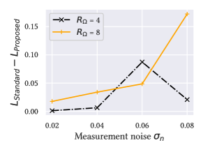
Figure 3: The difference in decibels between the test set loss of Standard VarNet, $L_{Standard}$, and the proposed Denoising VarNet, $L_{Proposed}$, is shown for the benchmark training method. All differences are positive, showing that Denoising VarNet outperforms Standard VarNet, especially for large $\sigma_{n}$.

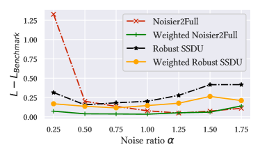
Figure 4: The robustness of Noisier2Full, Robust SSDU and their weighted versions to $\alpha$ at $R_{\Omega}=8$ and $\sigma_{n}=0.06$. The difference in decibels between the test set loss $L$ and the best-case benchmark $L_{Benchmark}$ is shown. The weighted versions are substantially more robust, especially for small $\alpha$.

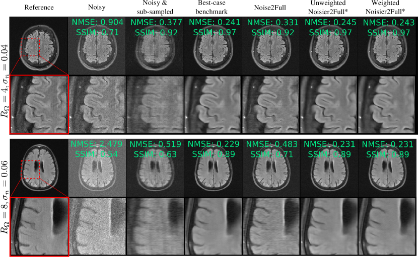
Figure 5: Reconstructions when fully sampled, noisy data is available for training. “Noisy” and “Noisy & sub-sampled” refer to the RSS reconstruction of $y_{0,s}+n_{s}$ and $M_{\Omega_{s}}(y_{0,s}+n_{s})$ respectively. While there is clear noise in Noise2Full’s reconstruction, the proposed methods, which are indicated with an asterisk, perform very similarly to the best-case benchmark.

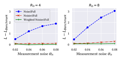
Figure 6: The test set loss in decibels for methods that use noisy, fully-sampled training data. Weighted Noisier2Full performs comparably with the best-case benchmark for all $\sigma_{n}$. We emphasize that the flatness does not imply that the test set loss is unchanged for changing $\sigma_{n}$, as the best-case benchmark test set loss is different for each $\sigma_{n}$.

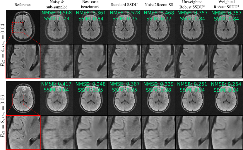
Figure 7: Example reconstructions for networks trained on noisy, sub-sampled data. The proposed methods, highlighted with an asterisk, perform very similarly to the best-case benchmark, even at $R_{\Omega}=8$.

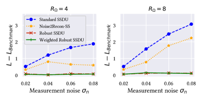
Figure 8: The test set loss in decibels for methods that use noisy, sub-sampled training data. The difference between the loss and the best-case benchmark is shown.

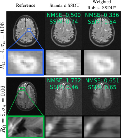
Figure 9: Clinical regions of interest annotated via fastMRI+ [36] at $\sigma_{n}=0.06$. The top image shows a lacunar infarct and the bottom shows a resection cavity. The proposed method Weighted Robust SSDU has improved sharpness compared to Standard SSDU, which has substantial reconstruction errors arising from the measurement noise.

V-A Evaluation of Denoising VarNet

To evaluate the performance of the proposed Denoising VarNet architecture, we trained the best-case baseline for Standard VarNet with 10 cascades and the Denoising VarNet with 5 cascades, so that they had roughly the same number of parameters. Fig. 3 shows that Denoising VarNet outperforms Standard VarNet on the test set for all considered $R_{\Omega}$ and $\sigma_{n}$, especially for more challenging acceleration factors and noise levels.

V-B Robustness to $\alpha$

To evaluate the robustness to $\alpha$, we trained Noisier2Full, Robust SSDU and their weighted variants for $\alpha$ between 0.25 to 1.75 in steps of 0.25. We focused solely on the case where $R_{\Omega}=8$ and $\sigma_{n}=0.06$. The performance on the test set is shown in Fig. 4, which shows that the weighted versions are considerably more robust. The weighted and unweighted minima were at $\alpha=1$ and $1.25$ for Noisier2Full and $\alpha=0.75$ and $0.5$ respectively. We employed these values of $\alpha$ for all experiments in Section V-C and V-D; we assumed that the tuned $\alpha$ at $R_{\Omega}=8$ and $\sigma_{n}=0.06$ is a reasonable approximation of the optimum for every every evaluated $R_{\Omega}$ and $\sigma_{n}$.

V-C Task A: Fully sampled, noisy training data

Fig. 6 shows the how the test set loss of networks trained on fully sampled, noisy data compares with the best-case benchmark. Noise2Full’s performance significantly degrades as $\sigma_{n}$ increases: for $R_{\Omega}=8$ and $\sigma_{n}=0.08$, Noise2Full’s test set loss is approximately double that of the best-case benchmark. In contrast, Weighted Noisier2Full performs similarly to the benchmark: for all $\sigma_{n}$ and $R_{\Omega}$, Weighted Noisier2Full was within 0.09dB of the best-case benchmark. The performance of unweighted Noisier2Full was slightly poorer than the weighted version, especially for high noise levels at the more challenging acceleration factor $R_{\Omega}=8$. Two reconstruction examples are shown in Fig. 5. Here, and throughout this paper, the example reconstructions show the image domain RSS cropped to a central $320\times 320$ region. The k-space Normalized Mean-Squared Error (NMSE) and Structural Similarity (SSIM) [37] are also shown, where the SSIM is computed on the magnitude image with the background excluded via the mask from the ESPIRiT algorithm [38], which we implemented with the BART toolbox [39].

V-D Task B: Sub-sampled, noisy training data

Fig. 8 shows the test set loss for the methods designed for sub-sampled, noisy training data. The weighted and unweighted variants of the proposed Robust SSDU performed within 0.17dB of the best-case benchmark, despite only having access to noisy, sub-sampled training data. Noise2Recon-SS performs well in some cases, particularly at $R_{\Omega}=4$, but is consistently outperformed by both variants of Robust SSDU. Fig. 7 shows example reconstructions, demonstrating similar performance to the best-case benchmark qualitatively. Fig. 9 compares Standard SSDU and Weighted Robust SSDU using clinical expert bounding boxes from fastMRI+ [36], which shows that the proposed method has substantially enhanced pathology visualization.

VI Discussion and conclusions

Fig. 3 shows that the proposed Denoising VarNet consistently outperforms the Standard VarNet architecture. We understand this to be a consequence of the difference between the distributions of errors due to sub-sampling or measurement noise: the Standard VarNet removes both contributions to the error in a single U-net per cascade, while the Denoising VarNet simplifies the task by decomposing the contributions to the error, so that each of the two U-nets per cascade are specialized for the two distinct error distributions.

The improvement in robustness for the weighted versions, shown in Fig. 4, is especially prominent for small $\alpha$. For instance, at $\alpha=0.25$, the unweighted variant of Noisier2Full is 1.3dB from the benchmark, while the weighted variant is only 0.072dB away. For large $\alpha$ the $\alpha$-based weighting is closer to 1, so weighted Noisier2Full tends to the unweighted method and the difference in performance is small. For instance, when $\alpha=1.75$, the $\alpha$-based weighting is $1.33$, so has a relatively marginal effect. Although the performance of the methods are reasonably similar for tuned $\alpha$, we recommend using the weighted version in practice due to its improved robustness to $\alpha$.

The examples in figures 5, 7 and 9 show that proposed methods are qualitatively very similar to the best-case benchmark, and substantially improve over methods without denoising, whose reconstructions are visibly corrupted with measurement noise. The examples exhibit some loss of detail and blurring at tissue boundaries, especially at $R_{\Omega}=8$. However, the extent of detail loss is similar in the benchmark, indicating that the loss of detail is not a limitation of the proposed methods. Rather, the qualitative performance is limited by the other factors such as the architecture, dataset and choice of loss function. This can also be explained in part by noting that the high-frequency regions of k-space, which provide fine details, typically have smaller signal so are particularly challenging to recover in the presence of significant measurement noise.

The pseudo-denoising effect described in Section III is visible in Fig. 5, which shows less noise in Noise2Full than Noisy. We note that the NMSE of Noisy is roughly 4 and 8 times larger than Noise2Full for $R_{\Omega}=4,8$ respectively, consistent with the theoretical finding that Noise2Full does not remove the measurement noise in the input. A comparison of figures 6 and 8 shows that Standard SSDU performs very similarly to Noise2Full quantitatively, exhibiting a similar pseudo-denoising effect.

Although Noise2Recon-SS improves over Standard SSDU, there is a substantial difference between its performance and the proposed Robust SSDU both qualitatively and quantitatively. In [20], Noise2Recon-SS was not compared with a best-case benchmark; it was only shown to have improved performance compared to Standard SSDU, consistent with the results here. The experimental evaluation in [20] focused on robustness to Out of Distribution (OOD) shifts, where the training and inference measurement noise variances not necessarily the same. Another difference is that Noise2Recon-SS’s simulated noise in [20] had standard deviation randomly selected from a fixed range, while the experiments here fixed the simulated noise standard deviation so that it could be properly compared with the proposed methods.

Robust SSDU requires only a few additional cheap computational steps compared to standard training: the addition or multiplication of the further noise and sub-sampling mask respectively, and the $\alpha$-based correction at inference. Accordingly, the compute time and memory requirements of the proposed methods was found to be very similar to Noise2Full or Standard SSDU. In contrast, Noise2Recon-SS uses both $M_{\Lambda_{t}}y_{t}$ and $y_{t}+M_{\Omega_{t}}\widetilde{n}_{t}$ as the network inputs at training, so requires twice as many forward passes to train the network compared to Robust SSDU. Accordingly, we found that Noise2Recon-SS required approximately twice as much memory and took around two times longer per epoch as the proposed methods.

Another existing method designed for noisy, sub-sampled training data is Robust Equivariant Imaging (REI) method [40, 41]. We did not compare with REI as it was designed for reconstruction tasks with a fixed sampling pattern: the $\Omega_{t}$ was the same for all $t$. This sampling set assumption is central to their use of equivariance, and contrasts with the methods proposed here, which assume that the sampling mask is an instance of a random variable that satisfies $p_{j}>0$ everywhere. However, REI’s suggestion to use Stein’s Unbiased Risk Estimate (SURE) [42] to remove measurement noise would be feasible in combination with SSDU and warrants further investigation in future work.

In [16], an untrained denoising algorithm or pre-trained denoising network was appended to a reconstruction network, which was found to perform well in practice despite not modeling the task-specific noise characteristics [43]. To test the former, we denoised the magnitude image output of Standard SSDU with BM3D [44]. We found that this approach was not competitive with the proposed methods: for instance, at $R_{\Omega}=8$ and $\sigma_{n}=0.06$, we found that the NMSE improvement compared to Standard SSDU was only around 0.5dB. Although appending a pre-trained denoising network to a reconstruction network was beyond the scope of this work, we note that employing transfer learning in conjunction with Robust SSDU to fine-tune a pre-trained denoisier to a specific dataset and noise model is a potential direction for future work.

The theoretical work presented in this paper only applies to the case of $\ell_{2}$ minimization, which can lead to blurry reconstructions. However, it has been established that Standard SSDU can be applied with other losses such as an entry-wise mixed $\ell_{1}$-$\ell_{2}$ loss in k-space [13]. We have found that Robust SSDU with an $\ell_{2}$ loss on $\Lambda\cap\Omega$ and mixed $\ell_{1}$-$\ell_{2}$ loss on $\Omega\setminus\Lambda$ also performs competitively with a suitable benchmark in practice (results not shown for brevity). Future work includes establishing whether Robust SSDU can be modified to be applicable to other loss functions, including potentially losses on the RSS image.

It was assumed in this paper that the measurement noise is white with known variance. Future work includes evaluating the performance of the proposed methods for the more realistic case where the measurement noise has non-trivial covariance matrix and is estimated retrospectively. It would also be desirable to develop an approach that automatically tunes $\alpha$ and the distribution of $M_{\Lambda}$, whose optimal values are specific to the noise model, $M_{\Omega}$ distribution and dataset.

VII Appendices

VII-A Proof of SSDU variant on $M_{\Omega}$

This appendix proves Claim 1 using a similar approach to Appendix B of [18]. Minimization according to (15) yields a network that satisfies

$$\mathds{E}[M_{\Omega}(f_{\theta^{*}}(\widetilde{Y})-Y)|\widetilde{Y}]=0$$ (20)

We split the conditional expectation into two cases: $\widetilde{Y}_{j}\neq 0$ and $\widetilde{Y}_{j}=0$.

Case 1 ($\mathds{E}[m_{j}(f_{\theta^{*}}(\widetilde{Y})_{j}-Y_{j})|\widetilde{Y}_{j}\neq 0]$): When $\widetilde{Y}_{j}\neq 0$, the measurement model implies that $m_{j}=1$ and $Y_{j}=Y_{0,j}+N_{j}$. Therefore

$$\mathds{E}[m_{j}(f_{\theta^{*}}(\widetilde{Y})_{j}-Y_{j})|\widetilde{Y}_{j}\neq 0]\\ =\mathds{E}[f_{\theta^{*}}(\widetilde{Y})_{j}-Y_{0,j}-N_{j}|\widetilde{Y}_{j}\neq 0]$$ (21)

Case 2 ($\mathds{E}[m_{j}(f_{\theta^{*}}(\widetilde{Y})_{j}-Y_{j})|\widetilde{Y}_{j}=0]$): We can use the result derived from equation (27) to (29) in [18], with $Y_{0,j}$ replaced by $Y_{0,j}+N_{j}$:

$$\mathds{E}[m_{j}(f_{\theta^{*}}(\widetilde{Y})_{j}-Y_{j})|\widetilde{Y}_{j}=0]\\ =\mathds{E}[f_{\theta^{*}}(\widetilde{Y})_{j}-Y_{0,j}-N_{j}|\widetilde{Y}_{j}=0]\cdot(1-k_{j})$$ (22)

where

$$k_{j}=\mathds{P}[Y_{j}=0|\widetilde{Y}_{j}=0]=\frac{1-p_{j}}{1-\widetilde{p}_{j}p_{j}}.$$ (23)

Combining Cases 1 and 2: Consider the candidate

$$\mathds{E}[m_{j}(f_{\theta^{*}}(\widetilde{Y})_{j}-Y_{j})|\widetilde{Y}_{j}]$$

$$=\{1-k_{j}(1-\widetilde{m}_{j}m_{j})\}\mathds{E}[f_{\theta^{*}}(\widetilde{Y})_{j}-Y_{0,j}-N_{j}|\widetilde{Y}_{j}].$$ (24)

To verify that this expression is correct, we can check that it is consistent with Cases 1 and 2. For Case 1: if $\widetilde{Y}_{j}\neq 0$, $\widetilde{m}_{j}m_{j}=1$ and the term in curly brackets is $1$, so (24) is consistent with (21). For Case 2: if $\widetilde{Y}_{j}=0$, $\widetilde{m}_{j}m_{j}=0$ and the term in curly brackets is $1-k_{j}$, so (24) is consistent with (22) as required. By (20),

$$\{1-k_{j}(1-\widetilde{m}_{j}m_{j})\}\mathds{E}[f_{\theta^{*}}(\widetilde{Y})_{j}-Y_{0,j}-N_{j}|\widetilde{Y}_{j}]=0$$

The term in the curly brackets is non-zero for all $j$ if $1-k_{j}$ is non-zero for $j\notin\Omega\cap\Lambda$, which true when (7) and (8) hold, where we note that the special case $\widetilde{p}_{j}=p_{j}=1$ is also allowed since $\widetilde{m}_{j}m_{j}=1$ always. Given this assumption, dividing by the term in the curly brackets:

$$\mathds{E}[f_{\theta^{*}}(\widetilde{Y})_{j}-Y_{0,j}-N_{j}|\widetilde{Y}_{j}]=0.$$ (25)

Vectorizing gives the required result. $\blacksquare$

VII-B Proof of weighted Noisier2Full

To compute the unknown

$$\nabla_{\theta}\mathds{E}\left[\left\|\hat{Y}_{Nr2F}-Y_{0}\right\|^{2}_{2}|\widetilde{Y}\right]$$

in terms of the known $Y_{0}+N$, we compute the contributions to the loss in $\Omega$ and $\Omega^{c}$ separately, shown in lemmas 1 and 2 respectively.

Lemma 1.

Consider the random variables $Y=M_{\Omega}(Y_{0}+N)$ and $\widetilde{Y}=Y+M_{\Omega}\widetilde{N}$, where $N$ and $\widetilde{N}$ are zero-mean Gaussian distributed with variances $\sigma_{n}^{2}$ and $\alpha^{2}\sigma_{n}^{2}$ respectively. For an arbitrary function $f_{\theta}$,

$$\nabla_{\theta}\mathds{E}\left[\left\|M_{\Omega}\left(\hat{Y}_{Nr2F}-Y_{0}\right)\right\|^{2}_{2}|\widetilde{Y}\right]\\ =\nabla_{\theta}\mathds{E}\left[\left\|\frac{1+\alpha^{2}}{\alpha^{2}}M_{\Omega}(f_{\theta}(\widetilde{Y})-Y)\right\|^{2}_{2}|\widetilde{Y}\right].$$ (26)

Proof.

Using $M_{\Omega}\widetilde{Y}=M_{\Omega}(Y+\widetilde{N})$ and $M_{\Omega}Y_{0}=M_{\Omega}(Y-N)$, the left-hand-side of (26) is

$$\nabla_{\theta}\mathds{E}\left[\left\|M_{\Omega}\left(\frac{(1+\alpha^{2})f_{\theta}(\widetilde{Y})-\widetilde{Y}}{\alpha^{2}}-Y_{0}\right)\right\|^{2}_{2}|\widetilde{Y}\right]$$

$$=\nabla_{\theta}\mathds{E}\left[\left\|M_{\Omega}\left(\frac{(1+\alpha^{2})f_{\theta}(\widetilde{Y})-Y-\widetilde{N}}{\alpha^{2}}-Y+N\right)\right\|^{2}_{2}|\widetilde{Y}\right]$$

$$=\nabla_{\theta}\mathds{E}\left[\left\|M_{\Omega}\left(\frac{1+\alpha^{2}}{\alpha^{2}}(f_{\theta}(\widetilde{Y})-Y)+N-\frac{\widetilde{N}}{\alpha^{2}}\right)\right\|^{2}_{2}|\widetilde{Y}\right]$$

$$=\nabla_{\theta}\mathds{E}\left[\left\|\frac{1+\alpha^{2}}{\alpha^{2}}M_{\Omega}(f_{\theta}(\widetilde{Y})-Y)\right\|^{2}_{2}|\widetilde{Y}\right]$$

$$\hskip 22.76228pt+\frac{1+\alpha^{2}}{\alpha^{2}}\nabla_{\theta}\mathds{E}\left[2f_{\theta}(\widetilde{Y})^{H}M_{\Omega}\left(N-\frac{\widetilde{N}}{\alpha^{2}}\right)|\widetilde{Y}\right]$$ (27)

where all the terms in the expansion of the $\ell_{2}$ norm in the last step that are not dependent on $\theta$ have been zeroed by $\nabla_{\theta}$. Now we show that the second term on the right-hand-side of (27) is zero. Lemma 3.1 from [19] shows that

$$\mathds{E}[M_{\Omega}\widetilde{N}|\widetilde{Y}]=\alpha^{2}\mathds{E}[M_{\Omega}N|\widetilde{Y}].$$ (28)

where $M_{\Omega}$ is included as the result only applies to sampled terms. Therefore

$$\mathds{E}\left[f_{\theta}(\widetilde{Y})^{H}M_{\Omega}\left(N-\frac{\widetilde{N}}{\alpha^{2}}\right)|\widetilde{Y}\right]\\ =f_{\theta}(\widetilde{Y})^{H}\mathds{E}\left[M_{\Omega}\left(N-\frac{\widetilde{N}}{\alpha^{2}}\right)|\widetilde{Y}\right]=0$$

where the conditional dependence on $\widetilde{Y}$ allows the removal of $f_{\theta}(\widetilde{Y})$ from the expectation. Therefore the right-hand-side of (27) equals the right-hand-side of (26) as required. ∎

Lemma 2.

Consider the random variables $Y$ and $\widetilde{Y}$ as defined in Lemma 1. For an arbitrary function $f_{\theta}$,

$$\nabla_{\theta}\mathds{E}\left[\left\|M_{\Omega^{c}}(\hat{Y}_{Nr2F}-Y_{0})|\widetilde{Y}\right\|^{2}_{2}\right]\\ =\nabla_{\theta}\mathds{E}\left[\left\|M_{\Omega^{c}}(f_{\theta}(\widetilde{Y})-Y_{0}-N)\right\|^{2}_{2}|\widetilde{Y}\right].$$ (29)

Proof.

Since $M_{\Omega^{c}}\hat{Y}_{Nr2F}=M_{\Omega^{c}}f_{\theta}(\widetilde{Y})$, the left-hand-side of (29) is

$$\nabla_{\theta}\mathds{E}\left[\left\|M_{\Omega^{c}}(f_{\theta}(\widetilde{Y})-Y_{0})\right\|^{2}_{2}|\widetilde{Y}\right]$$

$$=\nabla_{\theta}\mathds{E}\left[\left\|M_{\Omega^{c}}(f_{\theta}(\widetilde{Y})-Y_{0}-N+N)\right\|^{2}_{2}|\widetilde{Y}\right]$$

$$=\nabla_{\theta}\mathds{E}\left[\left\|M_{\Omega^{c}}(f_{\theta}(\widetilde{Y})-Y_{0}-N)\right\|^{2}_{2}+2f_{\theta}(\widetilde{Y})^{H}M_{\Omega^{c}}N|\widetilde{Y}\right]$$ (30)

where again all the terms not dependent on $\theta$ have been zeroed by $\nabla_{\theta}$. The second term is

$$\mathds{E}\left[f_{\theta}(\widetilde{Y})^{H}M_{\Omega^{c}}N|\widetilde{Y}\right]=f_{\theta}(\widetilde{Y})^{H}\mathds{E}\left[M_{\Omega^{c}}N|\widetilde{Y}\right]=0$$

where, as in (12), we have used the independence of $N$ from $\widetilde{Y}$ when $j\notin\Omega$. Therefore (30) equals the right-hand-side of (29) as required. ∎

To find the $\ell_{2}$ error of $\hat{Y}_{Nr2F}$, we use $M_{\Omega}+M_{\Omega^{c}}=\mathds{1}$ and sum the results from lemmas 1 and 2:

$$\nabla_{\theta}\mathds{E}\left[\left\|\hat{Y}_{Nr2F}-Y_{0}\right\|^{2}_{2}|\widetilde{Y}\right]$$

$$=\nabla_{\theta}\mathds{E}\left[\left\|(M_{\Omega}+M_{\Omega^{c}})(\hat{Y}_{Nr2F}-Y_{0})\right\|^{2}_{2}|\widetilde{Y}\right]$$

$$=\nabla_{\theta}\mathds{E}\left[\left\|\left(\frac{1+\alpha^{2}}{\alpha^{2}}M_{\Omega}+M_{\Omega^{c}}\right)(f_{\theta}(\widetilde{Y})-Y_{0}-N)\right\|^{2}_{2}|\widetilde{Y}\right]$$

as required.

VII-C Proof of weighted Robust SSDU

Analogous to Appendix VII-B, to compute the unknown

$$\nabla_{\theta}\mathds{E}\left[\left\|\hat{Y}_{RSSDU}-Y_{0}\right\|^{2}_{2}|\widetilde{Y}\right]$$

in terms of the known sub-sampled, noisy $Y$, we compute the contributions to the loss from $\Lambda\cap\Omega$ and $(\Lambda\cap\Omega)^{c}$ separately. For the contribution from $\Lambda\cap\Omega$, an identical approach to the proof in Lemma 1 can be used with $\Omega$ replaced by $\Lambda\cap\Omega$, so that

$$\nabla_{\theta}\mathds{E}\left[\left\|M_{\Lambda\cap\Omega}\left(\hat{Y}_{RSSDU}-Y_{0}\right)\right\|^{2}_{2}|\widetilde{Y}\right]\\ =\nabla_{\theta}\mathds{E}\left[\left\|\frac{1+\alpha^{2}}{\alpha^{2}}M_{\Lambda\cap\Omega}(f_{\theta}(\widetilde{Y})-Y)\right\|^{2}_{2}|\widetilde{Y}\right]$$ (31)

The following lemma shows how the remaining loss, which is computed on $\Omega\setminus\Lambda$, can be used to estimate the target ground truth loss, which is over $(\Lambda\cap\Omega)^{c}$.

Lemma 3.

Consider the random variables $Y=M_{\Omega}(Y_{0}+N)$ and $\widetilde{Y}=M_{\Lambda\cap\Omega}(Y+\widetilde{N})$, where $N$ and $\widetilde{N}$ are zero-mean Gaussian distributed with variances $\sigma_{n}^{2}$ and $\alpha^{2}\sigma_{n}^{2}$ respectively. For an arbitrary function $f_{\theta}$,

$$\nabla_{\theta}\mathds{E}\left[\left\|M_{(\Lambda\cap\Omega)^{c}}(\hat{Y}_{RSSDU}-Y_{0})\right\|^{2}_{2}|\widetilde{Y}\right]\\ =\nabla_{\theta}\mathds{E}\left[\left\|\mathcal{P}^{1/2}M_{\Omega\setminus\Lambda}(f_{\theta}(\widetilde{Y})-Y)\right\|^{2}_{2}|\widetilde{Y}\right]$$ (32)

where $\mathcal{P}$ is defined in (19).

Proof.

Since $M_{(\Lambda\cap\Omega)^{c}}\hat{Y}_{RSSDU}=M_{(\Lambda\cap\Omega)^{c}}f_{\theta}(\widetilde{Y})$, the left-hand-side of (32) is

$$\nabla_{\theta}\mathds{E}\left[\left\|M_{(\Lambda\cap\Omega)^{c}}(f_{\theta}(\widetilde{Y})-Y_{0})\right\|^{2}_{2}|\widetilde{Y}\right]\\ =\nabla_{\theta}\mathds{E}\left[\left\|M_{(\Lambda\cap\Omega)^{c}}(f_{\theta}(\widetilde{Y})-Y_{0}-N)\right\|^{2}_{2}|\widetilde{Y}\right]$$

where Lemma 2 with $\Omega^{c}$ replaced by $(\Lambda\cap\Omega)^{c}$ has been used. Using $|\cdot|^{2}$ to denote the entry-wise magnitude squared, we can write

$$\nabla_{\theta}\mathds{E}\left[\left\|M_{(\Lambda\cap\Omega)^{c}}(f_{\theta}(\widetilde{Y})-Y_{0}-N)\right\|^{2}_{2}|\widetilde{Y}\right]$$

$$=\nabla_{\theta}\mathds{E}\left[1_{q}^{T}M_{(\Lambda\cap\Omega)^{c}}|f_{\theta}(\widetilde{Y})-Y_{0}-N|^{2}|\widetilde{Y}\right],$$

where $1_{q}$ is a $q$-dimensional vector of ones. Eqn. (32) from [18] shows that the conditional expectation of $f_{\theta}(\widetilde{Y})-Y$ on $M_{(\Lambda\cap\Omega)^{c}}$ and $M_{\Omega\setminus\Lambda}$ is related by a factor $\mathcal{P}$. By repeating that derivation with all instances of $f_{\theta}(\widetilde{Y})-Y$ trivially replaced with $|f_{\theta}(\widetilde{Y})-Y_{0}-N|^{2}$, a similar relationship can be derived for the latter, yielding the same $\mathcal{P}$ factor: see [18]. Therefore

$$\nabla_{\theta}\mathds{E}\left[1_{q}^{T}M_{(\Lambda\cap\Omega)^{c}}|f_{\theta}(\widetilde{Y})-Y_{0}-N|^{2}|\widetilde{Y}\right]$$

$$=\nabla_{\theta}\mathds{E}\left[1_{q}^{T}\mathcal{P}M_{\Omega\setminus\Lambda}|f_{\theta}(\widetilde{Y})-Y_{0}-N|^{2}|\widetilde{Y}\right]$$

$$=\nabla_{\theta}\mathds{E}\left[\left\|\mathcal{P}^{1/2}M_{\Omega\setminus\Lambda}(f_{\theta}(\widetilde{Y})-Y)\right\|^{2}_{2}|\widetilde{Y}\right].$$

as required. ∎

To find the $\ell_{2}$ error of $\hat{Y}_{RSSDU}$, we use $M_{\Lambda\cap\Omega}+M_{(\Lambda\cap\Omega)^{c}}=\mathds{1}$ and sum (31) and (32):

$$\nabla_{\theta}\mathds{E}\left[\left\|\hat{Y}_{RSSDU}-Y_{0}\right\|^{2}_{2}|\widetilde{Y}\right]$$

$$=\nabla_{\theta}\mathds{E}\left[\left\|(M_{\Lambda\cap\Omega}+M_{(\Lambda\cap\Omega)^{c}})(\hat{Y}_{Nr2F}-Y_{0})\right\|^{2}_{2}|\widetilde{Y}\right]$$

$$=\nabla_{\theta}\mathds{E}\left[\left\|\left(\frac{1+\alpha^{2}}{\alpha^{2}}M_{\Lambda\cap\Omega}+\mathcal{P}^{1/2}M_{\Omega\setminus\Lambda}\right)(f_{\theta}(\widetilde{Y})-Y)\right\|^{2}_{2}|\widetilde{Y}\right]$$

as required.

References

- [1] A. Bustin, N. Fuin, R. M. Botnar, and C. Prieto, “From compressed-sensing to artificial intelligence-based cardiac MRI reconstruction,” Frontiers in cardiovascular medicine, vol. 7, p. 17, 2020.
- [2] K. P. Pruessmann, M. Weiger, M. B. Scheidegger, and P. Boesiger, “SENSE: sensitivity encoding for fast MRI.,” Magnetic resonance in medicine, vol. 42, pp. 952–62, nov 1999.
- [3] M. Lustig, D. Donoho, and J. M. Pauly, “Sparse MRI: The application of compressed sensing for rapid MR imaging,” Magnetic Resonance in Medicine, vol. 58, pp. 1182–1195, dec 2007.
- [4] J. C. Ye, “Compressed sensing MRI: a review from signal processing perspective,” BMC Biomedical Engineering, vol. 1, p. 8, dec 2019.
- [5] S. Wang, Z. Su, L. Ying, X. Peng, S. Zhu, F. Liang, D. Feng, and D. Liang, “Accelerating magnetic resonance imaging via deep learning,” in 2016 IEEE 13th International Symposium on Biomedical Imaging (ISBI), pp. 514–517, 2016.
- [6] K. Kwon, D. Kim, and H. Park, “A parallel MR imaging method using multilayer perceptron,” Medical physics, vol. 44, no. 12, pp. 6209–6224, 2017.
- [7] K. Hammernik, T. Klatzer, E. Kobler, M. P. Recht, D. K. Sodickson, T. Pock, and F. Knoll, “Learning a variational network for reconstruction of accelerated MRI data,” Magnetic resonance in medicine, vol. 79, no. 6, pp. 3055–3071, 2018.
- [8] M. Uecker, S. Zhang, D. Voit, A. Karaus, K.-D. Merboldt, and J. Frahm, “Real-time MRI at a resolution of 20 ms,” NMR in Biomedicine, vol. 23, no. 8, pp. 986–994, 2010.
- [9] H. Haji-Valizadeh, A. A. Rahsepar, J. D. Collins, E. Bassett, T. Isakova, T. Block, G. Adluru, E. V. DiBella, D. C. Lee, J. C. Carr, et al., “Validation of highly accelerated real-time cardiac cine MRI with radial k-space sampling and compressed sensing in patients at 1.5 T and 3T,” Magnetic resonance in medicine, vol. 79, no. 5, pp. 2745–2751, 2018.
- [10] Y. Lim, Y. Zhu, S. G. Lingala, D. Byrd, S. Narayanan, and K. S. Nayak, “3D dynamic MRI of the vocal tract during natural speech,” Magnetic resonance in medicine, vol. 81, no. 3, pp. 1511–1520, 2019.
- [11] J. I. Tamir, X. Y. Stella, and M. Lustig, “Unsupervised deep basis pursuit: Learning reconstruction without ground-truth data,” in ISMRM annual meeting, 2019.
- [12] P. Huang, C. Zhang, H. Li, S. K. Gaire, R. Liu, X. Zhang, X. Li, and L. Ying, “Deep MRI reconstruction without ground truth for training,” in ISMRM annual meeting, 2019.
- [13] B. Yaman, S. A. H. Hosseini, S. Moeller, J. Ellermann, K. Uğurbil, and M. Akçakaya, “Self-supervised learning of physics-guided reconstruction neural networks without fully sampled reference data,” Magnetic resonance in medicine, vol. 84, no. 6, pp. 3172–3191, 2020.
- [14] H. K. Aggarwal, A. Pramanik, and M. Jacob, “ENSURE: Ensemble Stein’s unbiased risk estimator for unsupervised learning,” in IEEE International Conference on Acoustics, Speech and Signal Processing (ICASSP), pp. 1160–1164, 2021.
- [15] J. Obungoloch, J. R. Harper, S. Consevage, I. M. Savukov, T. Neuberger, S. Tadigadapa, and S. J. Schiff, “Design of a sustainable prepolarizing magnetic resonance imaging system for infant hydrocephalus,” Magnetic Resonance Materials in Physics, Biology and Medicine, vol. 31, pp. 665–676, 2018.
- [16] N. Koonjoo, B. Zhu, G. C. Bagnall, D. Bhutto, and M. Rosen, “Boosting the signal-to-noise of low-field MRI with deep learning image reconstruction,” Scientific reports, vol. 11, no. 1, p. 8248, 2021.
- [17] J. Schlemper, S. S. M. Salehi, C. Lazarus, H. Dyvorne, R. O’Halloran, N. de Zwart, L. Sacolick, J. M. Stein, D. Rueckert, M. Sofka, et al., “Deep learning MRI reconstruction in application to point-of-care MRI,” in Proc. Intl. Soc. Mag. Reson. Med, vol. 28, p. 0991, 2020.
- [18] C. Millard and M. Chiew, “A Theoretical Framework for Self-Supervised MR Image Reconstruction Using Sub-Sampling via Variable Density Noisier2Noise,” IEEE Transactions on Computational Imaging, vol. 9, pp. 707–720, 2023.
- [19] N. Moran, D. Schmidt, Y. Zhong, and P. Coady, “Noisier2Noise: Learning to denoise from unpaired noisy data,” in Proceedings of the IEEE/CVF Conference on Computer Vision and Pattern Recognition, pp. 12064–12072, 2020.
- [20] A. D. Desai, B. M. Ozturkler, C. M. Sandino, R. Boutin, M. Willis, S. Vasanawala, B. A. Hargreaves, C. Ré, J. M. Pauly, and A. S. Chaudhari, “Noise2Recon: Enabling SNR-robust MRI reconstruction with semi-supervised and self-supervised learning,” Magnetic Resonance in Medicine, 2023.
- [21] M. S. Hansen and P. Kellman, “Image reconstruction: an overview for clinicians,” Journal of Magnetic Resonance Imaging, vol. 41, no. 3, pp. 573–585, 2015.
- [22] J. Lehtinen, J. Munkberg, J. Hasselgren, S. Laine, T. Karras, M. Aittala, and T. Aila, “Noise2Noise: Learning image restoration without clean data,” arXiv preprint arXiv:1803.04189, 2018.
- [23] A. Krull, T.-O. Buchholz, and F. Jug, “Noise2void-learning denoising from single noisy images,” in Proceedings of the IEEE/CVF Conference on Computer Vision and Pattern Recognition, pp. 2129–2137, 2019.
- [24] J. Batson and L. Royer, “Noise2self: Blind denoising by self-supervision,” in International Conference on Machine Learning, pp. 524–533, PMLR, 2019.
- [25] T. Huang, S. Li, X. Jia, H. Lu, and J. Liu, “Neighbor2neighbor: Self-supervised denoising from single noisy images,” in Proceedings of the IEEE/CVF conference on computer vision and pattern recognition, pp. 14781–14790, 2021.
- [26] G. Zeng, Y. Guo, J. Zhan, Z. Wang, Z. Lai, X. Du, X. Qu, and D. Guo, “A review on deep learning MRI reconstruction without fully sampled k-space,” BMC Medical Imaging, vol. 21, no. 1, pp. 1–11, 2021.
- [27] F. Wang, H. Qi, A. De Goyeneche, R. Heckel, M. Lustig, and E. Shimron, “K-band: Self-supervised MRI Reconstruction via Stochastic Gradient Descent over K-space Subsets,” arXiv preprint arXiv:2308.02958, 2023.
- [28] S. Wiedemann and R. Heckel, “A deep learning method for simultaneous denoising and missing wedge reconstruction in cryogenic electron tomography,” arXiv preprint arXiv:2311.05539, 2023.
- [29] J. Zbontar, F. Knoll, A. Sriram, T. Murrell, Z. Huang, M. J. Muckley, A. Defazio, R. Stern, P. Johnson, M. Bruno, et al., “fastMRI: An open dataset and benchmarks for accelerated MRI,” arXiv preprint arXiv:1811.08839, 2018.
- [30] M. Lyu, L. Mei, S. Huang, S. Liu, Y. Li, K. Yang, Y. Liu, Y. Dong, L. Dong, and E. X. Wu, “M4Raw: A multi-contrast, multi-repetition, multi-channel MRI k-space dataset for low-field MRI research,” Scientific Data, vol. 10, no. 1, p. 264, 2023.
- [31] A. A. Hendriksen, D. M. Pelt, and K. J. Batenburg, “Noise2Inverse: Self-supervised deep convolutional denoising for tomography,” IEEE Transactions on Computational Imaging, vol. 6, pp. 1320–1335, 2020.
- [32] A. Sriram, J. Zbontar, T. Murrell, A. Defazio, C. L. Zitnick, N. Yakubova, F. Knoll, and P. Johnson, “End-to-end variational networks for accelerated MRI reconstruction,” in International Conference on Medical Image Computing and Computer-Assisted Intervention, pp. 64–73, Springer, 2020.
- [33] O. Ronneberger, P. Fischer, and T. Brox, “U-net: Convolutional networks for biomedical image segmentation,” in International Conference on Medical Image Computing and Computer-Assisted Intervention, pp. 234–241, Springer, 2015.
- [34] D. P. Kingma and J. Ba, “Adam: A method for stochastic optimization,” arXiv preprint arXiv:1412.6980, 2014.
- [35] B. Yaman, S. A. H. Hosseini, S. Moeller, J. Ellermann, K. Uğurbil, and M. Akçakaya, “Ground-truth free multi-mask self-supervised physics-guided deep learning in highly accelerated MRI,” in 2021 IEEE 18th International Symposium on Biomedical Imaging (ISBI), pp. 1850–1854, 2021.
- [36] R. Zhao, B. Yaman, Y. Zhang, R. Stewart, A. Dixon, F. Knoll, Z. Huang, Y. W. Lui, M. S. Hansen, and M. P. Lungren, “fastMRI+, Clinical pathology annotations for knee and brain fully sampled magnetic resonance imaging data,” Scientific Data, vol. 9, no. 1, p. 152, 2022.
- [37] Z. Wang, A. C. Bovik, H. R. Sheikh, and E. P. Simoncelli, “Image quality assessment: From error visibility to structural similarity,” IEEE Transactions on Image Processing, vol. 13, no. 4, pp. 600–612, 2004.
- [38] M. Uecker, P. Lai, M. J. Murphy, P. Virtue, M. Elad, J. M. Pauly, S. S. Vasanawala, and M. Lustig, “ESPIRiT-an eigenvalue approach to autocalibrating parallel MRI: Where SENSE meets GRAPPA,” Magnetic Resonance in Medicine, vol. 71, pp. 990–1001, mar 2014.
- [39] M. Uecker, J. I. Tamir, F. Ong, and M. Lustig, “The BART Toolbox for Computational Magnetic Resonance Imaging,” in ISMRM, 2016.
- [40] D. Chen, J. Tachella, and M. E. Davies, “Robust equivariant imaging: a fully unsupervised framework for learning to image from noisy and partial measurements,” in Proceedings of the IEEE/CVF Conference on Computer Vision and Pattern Recognition, pp. 5647–5656, 2022.
- [41] D. Chen, J. Tachella, and M. E. Davies, “Equivariant imaging: Learning beyond the range space,” in Proceedings of the IEEE/CVF International Conference on Computer Vision, pp. 4379–4388, 2021.
- [42] C. M. Stein, “Estimation of the Mean of a Multivariate Normal Distribution,” The Annals of Statistics, vol. 9, pp. 1135–1151, nov 1981.
- [43] P. Virtue and M. Lustig, “The Empirical Effect of Gaussian Noise in Undersampled MRI Reconstruction,” Tomography, vol. 3, pp. 211–221, dec 2017.
- [44] K. Dabov, A. Foi, V. Katkovnik, and K. Egiazarian, “Image denoising by sparse 3-D transform-domain collaborative filtering.,” IEEE transactions on image processing : a publication of the IEEE Signal Processing Society, vol. 16, pp. 2080–95, aug 2007.