M-LIO: Multi-lidar, multi-IMU odometry with sensor dropout tolerance

We present a robust system for state estimation that fuses measurements from multiple lidars and inertial sensors with GNSS data. To initiate the method, we use the prior GNSS pose information. We then perform incremental motion in real-time, which produces robust motion estimates in a global frame by fusing lidar and IMU signals with GNSS translation components using a factor graph framework. We also propose methods to account for signal loss with a novel synchronization and fusion mechanism. To validate our approach extensive tests were carried out on data collected using Scania test vehicles (5 sequences for a total of $\approx$ 7 Km). From our evaluations, we show an average improvement of 61% in relative translation and 42% rotational error compared to a state-of-the-art estimator fusing a single lidar/inertial sensor pair.

I Introduction

State estimation, which is a sub-problem of Simultaneous Localization and Mapping (SLAM), is a fundamental building block of autonomous navigation. To develop robust SLAM systems, proprioceptive (IMU – inertial measurement unit, wheel encoders) and exteroceptive (camera, lidar, GNSS – Global Navigation Satellite System) sensing are fused. Existing systems have achieved robust and accurate results [1, 2, 3]; however, state estimation in dynamic conditions and when there is measurement loss or noisy is still challenging.

Compared to visual SLAM, lidar-based SLAM has higher accuracy as lidar range measurements of up to 100m directly enable precise motion tracking. Moreover, owing to the falling cost of lidars, mobile platforms are increasingly equipped with multiple lidars [4, 5], to give complementary and complete $360^{\circ}$ sensor coverage (see Fig. 1, for our data collection platform). This also improves the density of measurements which may be helpful for state estimation in degenerate scenarios such as tunnels or straight highways. We can also estimate the reliability of a state estimator by computing the covariance of measurement errors produced from multiple lidar measurements.

Meanwhile, IMUs are low cost sensors which can be used to estimate a motion prior for lidar odometry by integrating the rotation rate and accelerometry measurements. However, IMUs suffer from bias instability and are susceptible to noise. An array of multiple IMUs (MIMUs) could provide enhanced signal accuracy with bias and noise compensation as well as increasing operational robustness to sensor dropouts. Multi-lidar odometry [6, 7] and MIMU odometry [8, 9] have been studied separately; however to the best of our knowledge the fusion of the combined set has not yet been explored.

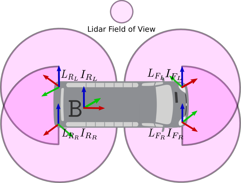
Figure 1: Illustration of the four lidars with their embedded IMUs positioned around the data collection vehicle. The vehicle base frame $\mathtt{{B}}$, is located at the center of the rear axle. The sensor frames of the lidars are: $\mathtt{L}_{{F_{R}}}$, $\mathtt{L}_{{F_{L}}}$, $\mathtt{L}_{{R_{R}}}$ and $\mathtt{L}_{{R_{L}}}$, whereas, the sensor frames of the IMUs are: $\mathtt{{I}}_{{F_{R}}}$, $\mathtt{{I}}_{{F_{L}}}$, $\mathtt{{I}}_{{R_{R}}}$ and $\mathtt{{I}}_{{R_{L}}}$. ${F_{R}}$: front-right, ${F_{L}}$: front-left, ${R_{R}}$: rear-right and ${R_{L}}$: rear-left.

I-A Motivation

As our vehicles are equipped with a GNSS system, we perform the state estimation in global frame and take advantage of it to limit the drift rate. Since GNSS information is unreliable in urban environments (‘urban canyon’) or in underground scenarios (such as mining) we also need to fuse information from onboard sensors (which might be susceptible to signal loss) to create robust state estimates.

To achieve this, we have identified two broad problems: Problem 1: State estimation over long time horizons with onboard sensing inherently suffers from drift. Problem 2: Sensor signals are susceptible to loss, due to networking or operational issues, which might affect reliability of the state estimates using onboard sensing.

In our work we have addressed Problem 1) by fusing the onboard state estimator with GNSS-based estimates. For Problem 2) we provide our formulation for the fusion of multiple lidars and MIMU to create robust signals under noisy conditions, which can give robustness both to failure of an individual lidar or IMU sensor as well as expanding the lidar field-of-view.

I-B Contribution

Our work is motivated by the broad literature in lidar and IMU based state estimation. Our proposed contributions are:

• Multi-lidar odometry using a single fused local submap and handling lidar dropout scenarios.

• MIMU fusion which compensates for the Coriolis effect and accounts for potential signal loss.

• A factor graph framework to jointly fuse multiple lidars, MIMUs and GNSS signals for robust state estimation in a global frame.

• Experimental results and verification using data collected from Scania vehicles with the sensor setup shown in Fig. 2, with FoV schematics similar to Fig. 1.

II Related Work

There have been multiple studies of lidar and IMU-based SLAM after the seminal LOAM paper by Zhang et al. [10] which is itself motivated by generalized-ICP work by Segal et al. [11]. In our discussion we briefly review the relevant literature.

II-A Direct tightly coupled multi-lidar odometry

To develop real-time SLAM systems simple edge and plane features are often extracted from the point clouds and tracked between frames for computational efficiency [3, 12, 13]. Using IMU propagation, motion priors can then be used to enable matching of point cloud features between key-frames. However, this principle cannot be applied to featureless environments. Hence, instead of feature engineering, the whole point cloud is often processed which has an analogy to processing the whole image in visual odometry methods such as LSD-SLAM, [14], which is known as direct estimation. To support direct methods, recently Xu et al. [15] proposed the ikd-tree in their Fast-LIO2 work which efficiently inserts, updates, searches and filters to maintain a local submap. The ikd-tree achieves its efficiency through “lazy delete” and “parallel tree re-balancing” mechanisms.

Furthermore, instead of point-wise operations the authors of Faster-LIO [16] proposed voxel-wise operations for point cloud association across frames and reported improved efficiency. In our work we also maintain an ikd-tree of the fused lidar measurements and tightly couple the relative lidar poses, IMU preintegration and GNSS prior in our propose estimator. Since, we jointly estimate the state based on the residual cost function built upon the multiple modalities we consider this a tightly coupled system.

While there have been many studies of state estimation using single lidar and IMU, there is limited literature available for fusing multi-lidar and MIMU systems. Our idea closely resembles M-LOAM [7], where state estimation with multiple lidars and calibration was performed. However, the working principles are different as M-LOAM is not a direct method and MIMU system is not considered in their work.

Finally, most authors do not address how to achieve reliability in situations of signal loss — an issue which is important for practical operational scenarios.

III Problem Statement

III-A Sensor platform and reference frames

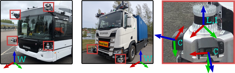
Figure 2: Reference frames conventions for our vehicle platform. The world frame $\mathtt{W}$ is a fixed frame, while the base frame $\mathtt{{B}}$, as shown in Fig. 1, is located at the rear axle center of the vehicle. Each sensor unit contains the two optical frames $\mathtt{C}$, an IMU frame, $\mathtt{I}$, and lidar frame $\mathtt{L}$. The cameras are shown for illustration only and they are not used for this work.

The sensor platform with its corresponding reference frames is shown in Fig. 2 along with the illustrative sensor fields-of-view in Fig. 1. Each of the sensor housings contain a lidar with a corresponding embedded IMU and two cameras. Although we do not use the cameras in this work they are illustrated here to show the full sensor setup. We used logs from a bus and a truck with similar sensor housings for our experiments. The two lower mounted modules from the rear, present in both the vehicles, are not shown here in the picture. The embedded IMUs within the lidar sensors are used to form the MIMU setup.

Now we describe the necessary notation and reference frames used in our system according to the convention of Furgale [17]. The vehicle base frame, $\mathtt{{B}}$ is located on the center of the rear-axle of the vehicle. Sensor readings from GNSS, lidars, cameras and IMUs are represented in their respective sensor frames as $\mathtt{G}$, $\mathtt{L}^{(k)}$, $\mathtt{C}^{(k)}$ and $\mathtt{I}^{(k)}$ respectively. Here, $k\in[F_{L},F_{R},R_{L},R_{R}]$ denotes the location of the sensor in the vehicle corresponding to front-left, front-right, rear-left and rear-right respectively. The GNSS measurements are reported in world fixed frame, $\mathtt{W}$ and transformed to $\mathtt{{B}}$ frame by performing a calibration routine outside the scope of this work. In our discussions the transformation matrix is denoted as, $\mathbf{T}=\left[\begin{array}[]{ll}\mathbf{R}_{3\times 3}&\mathbf{t}_{3\times 1}\\ \mathbf{0}^{\top}&1\end{array}\right]\in\mathrm{SE}(3)$ and $\mathbf{R}\mathbf{R}^{T}=\mathbf{I}_{3\times 3}$, since the rotation matrix is orthogonal.

III-B Problem formulation

Our primary goal is to estimate the position $\tensor[_{\mathtt{{W}}}]{\mathbf{t}}{{}_{\mathtt{{W}}\mathtt{{B}}}}$, orientation $\tensor[_{\mathtt{{W}}}]{\mathbf{R}}{{}_{\mathtt{{W}}\mathtt{{B}}}}$, linear velocity $\tensor[_{\mathtt{W}}]{\mathbf{v}}{{}_{\mathtt{{W}}\mathtt{{B}}}}$, and angular velocity $\tensor[_{\mathtt{W}}]{\boldsymbol{\omega}}{{}_{\mathtt{{W}}\mathtt{{B}}}}$, of the base frame $\mathtt{{B}}$, relative to the fixed world frame $\mathtt{W}$. Additionally, we also estimate the MIMU biases $\tensor[_{\mathtt{{B}}}]{\mathbf{b}}{{}^{g}},\;\tensor[_{\mathtt{{B}}}]{\mathbf{b}}{{}^{a}}$ expressed in $\mathtt{{B}}$ frame, as that is where it can be sensed. Hence, our estimate of vehicle’s state $\boldsymbol{x}_{i}$ at time $t_{i}$, is denoted as:

$$\boldsymbol{x}_{i}=\left[{\mathbf{R}}_{i},\;{\mathbf{t}}_{i},\;{\mathbf{v}}_{i},\;{\boldsymbol{\omega}}_{i},\;\mathbf{b}^{a}_{i},\;\mathbf{b}^{g}_{i}\right]\in\mathrm{SE}(3)\times\mathbb{R}^{15},$$ (1)

where, the corresponding measurements are in the frames mentioned above.

IV Methodology

IV-A Initialization

To provide an initial pose we use the GNSS measurements, $\tensor[_{\mathtt{W}}]{\mathbf{T}}{{}_{\mathtt{{\mathtt{W}\mathtt{G}}}}}$ and determine an initial estimate of the starting yaw and translation component, $\tensor[_{\mathtt{W}}]{\mathbf{t}}{{}_{\mathtt{{\mathtt{W}\mathtt{{B}}}}}}$, in UTM co-ordinates. The GNSS unit also provides IMU measurements in $\mathtt{G}$ frame using its internally embedded IMU, which is transformed to $\mathtt{{B}}$ frame. For gravity alignment we use the equations [18, Eq. 25, 26] to estimate roll and pitch after collecting IMU data when the vehicle is static for $t$ seconds according to the GNSS estimate. Subsequently, only the translation component $\tensor[_{\mathtt{W}}]{\mathbf{t}}{{}_{\mathtt{W}\mathtt{G}}}$, from the GNSS measurements are used.

Meanwhile, the noise processes and starting bias estimates for the embedded IMU sensors were characterized in advance by estimating the Allan Variance [19] parameters using logs collected while stationary.

IV-B Handling lossy signal scenario

To synchronizate the different signals and to handling signal drop we maintain individual buffer queues for each of the lidar and IMU signals. We read the data from the buffers in a FIFO approach and compare the header timestamps (within a threshold of 10 $\mathrm{m}\mathrm{s}$ for lidar and 1 $\mathrm{m}\mathrm{s}$ for IMU) to associate corresponding signals across different sensors as illustrated in Fig. 3. We add an age penalty for unused messages in the buffer queues to avoid unbounded queue growth. Unlike the default approximate time sync policy (in ROS) we ensure that data from a single sensor is returned if the other corresponding signals are available. As an illustration, in Fig. 3, let us assume we receive lossy lidar and IMU signals from our sensor setup. The green cells represent signal availability in the buffer queue, whereas the white cells represent signal loss. The signals are read in a FIFO approach and fused after corresponding associations are formed based on timestamps, which is shown with links between the messages in the middle part of Fig. 3. The right hand side illustrates the components of the fused signal. For example at $t_{2}$, the fused signals comprises of $F_{L}$ and $R_{R}$ signal only.

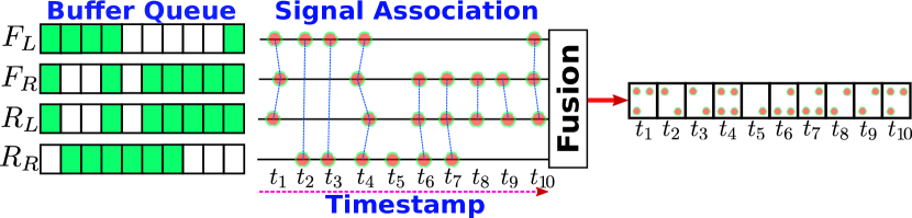
Figure 3: Handling and fusing lossy signals. Green cells denote available data while white cells denote a lost signal for the corresponding timestamp in the buffer queue.

IV-C Lidar fusion

After using the prior extrinsic calibration and signal correspondences we fuse the lidar data from the individual sensors in the $\mathtt{{B}}$ frame using a ikd-tree [15] and downsample them to a 5 $\mathrm{c}\mathrm{m}$ voxel resolution. To compensate for the motion distortion during a lidar scan, all points are projected to a pose corresponding to the beginning of the corresponding scan using IMU pre-integration [20] between the start and end of the lidar scan. We use the dual quaternion (DQ) operator to handle interpolation of translation and rotation components together using screw linear interpolation (ScLERP) [21]. Let, $\mathbf{p}_{t}$ be the the timestamp of a received lidar point at time $t\in[t_{i},t_{i+1}]$. The point can be transformed to the beginning of the scan as $\mathbf{T}_{\mathtt{L}_{i}\mathtt{L}_{t}}^{-1}\mathbf{p}_{t}$, where, $\mathbf{T}_{\mathtt{L}_{i}\mathtt{L}_{t}}$ can be recovered in DQ form as ($\mathbf{Q}$ is the DQ form of $\mathbf{T}$),

$$\mathbf{Q}_{\mathtt{L}_{i}\mathtt{L}_{t}}=\mathbf{Q}_{\mathtt{L}_{i}}\otimes(\mathbf{Q}_{\mathtt{L}_{i}}^{-1}\otimes\mathbf{Q}_{\mathtt{L}_{i+1}})^{\eta},\quad\eta=\frac{t-t_{i}}{t_{i+1}-t_{i}}.$$ (2)

IV-D IMU fusion

To create a robust IMU signal we fuse the available embedded IMUs as a set, which we call a MIMU. A naive approach for MIMU signal fusion would be averaging. Instead we use a MLE approach for the fusion [8].

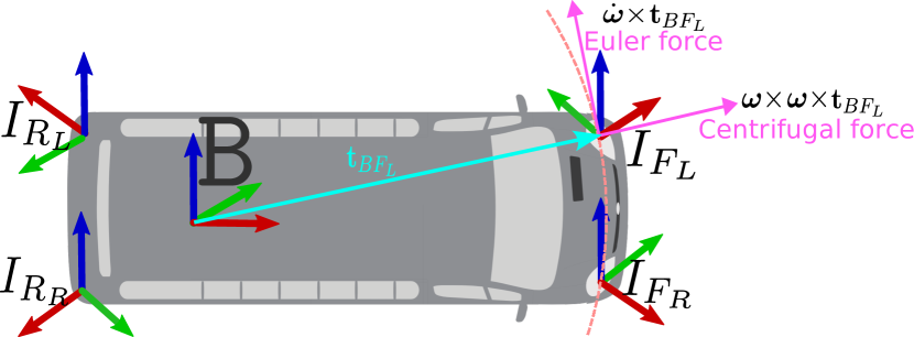
Figure 4: Illustration of IMU transformation with Coriolis force compensation.

IV-D1 IMU transformation with Coriolis compensation

Let, $\left[\mathbf{R}_{\mathtt{{B}}\mathtt{I}^{(k)}},\mathbf{t}_{\mathtt{{B}}\mathtt{I}^{(k)}}\right]$ be the calibration parameters between the $\mathtt{{B}}$ and the $k^{th}$ IMU frame, $\mathtt{I}^{(k)}$. $\mathbf{f}_{\mathtt{I}^{(k)}},\boldsymbol{\omega}_{\mathtt{I}^{(k)}}$ are the linear acceleration and angular velocity measurements for the $k^{th}$ IMU in its corresponding sensor frame, $\mathtt{I}^{(k)}$. Before the fusion of the MIMU signals, all the IMU measurements must be converted to the $\mathtt{{B}}$ frame by compensating for the Coriolis force illustrated in Fig. 4. Please note we have omitted $k$ superscript for brevity in rest of the discussion.

$$\mathbf{R}_{BI}^{-1}\mathbf{f}_{I}=\mathbf{f}_{B}+\underbrace{\boldsymbol{\omega}\times\left(\boldsymbol{\omega}\times\mathbf{t}_{BI}\right)}_{\text{Centrifugal force }}+\underbrace{\dot{\boldsymbol{\omega}}\times\mathbf{t}_{BI}}_{\text{Euler force }}$$ (3)

$$\mathbf{R}_{BI}^{-1}\mathbf{f}_{I} =\mathbf{f}_{B}+[\boldsymbol{\omega}]_{\times}[\boldsymbol{\omega}]_{\times}\mathbf{t}_{BI}+[\dot{\boldsymbol{\omega}}]_{\times}\mathbf{t}_{BI}$$ (4)

$$=\mathbf{f}_{B}+[\boldsymbol{\omega}]^{2}_{\times}\mathbf{t}_{BI}-[\mathbf{t}_{BI}]_{\times}\dot{\boldsymbol{\omega}},$$

where, $[\boldsymbol{.}]_{\times}$ is a skew-symmetric matrix and $[\mathbf{a}]_{\times}\mathbf{b}=-[\mathbf{b}]_{\times}\mathbf{a}$. In the first step of the IMU fusion, we orient all the IMU measurements in their respective sensor frames to $\mathtt{{B}}$ frame by applying eq. 4 with suitable calibration and noise parameters, estimated in advance while characterizing the IMUs.

IV-D2 Accelerometer signal model

From eq. 4 we can also derive the following signal model for an array of $K$ accelerometers, where $\mathbf{y}_{f}$ is the acceleration measurement vector and $\boldsymbol{\eta}^{f}$ is the measurement noise of the accelerometers:

$$\mathbf{y}_{f}=\mathbf{h}_{f}(\boldsymbol{\omega})+\mathbf{H}\Phi+\boldsymbol{\eta}^{f},$$ (5)

where,

IV-D3 Gyroscope signal model

The angular velocity is sensed by gyroscope on a rigid body is the same no matter where the sensor is located, the same applies for angular acceleration. Hence we can derive a simple model for the measurement vector $\mathbf{y}_{\omega}$, given the gyro measurement noise $\boldsymbol{\eta}^{\omega}$:

$$\mathbf{y}_{\omega} =\mathbf{h}_{\omega}(\boldsymbol{\omega})+\boldsymbol{\eta}^{\omega},$$ (7)

where, $\mathbf{h}_{\omega}(\boldsymbol{\omega})=\mathbf{1}_{K}\otimes\boldsymbol{\omega}$. Note that in eq. 7 we do not model the bias, as it has been done in IMU pre-integration. Here $\mathbf{1_{K}}$ is a column vector of ones and $\otimes$ is the kronecker product.

IV-D4 MIMU signal model

Concatenation of eq. 5 and eq. 7 yields:

$$\mathbf{y}=\mathbf{h}(\boldsymbol{\omega})+\mathbf{H\Phi}+\boldsymbol{\eta},$$ (8)

where,

and $\mathbf{0}_{m,n}$ denotes a zero matrix of size $m$ by $n$.

IV-D5 Maximum likelihood estimator

The objective is to use eq. 8 to form a log-likelihood function with the assumption of zero-mean Gaussian distribution of measurement noises:

$$L(\boldsymbol{\omega},\Phi)=\frac{1}{2}\left\|\mathbf{y}-\mathbf{h}(\boldsymbol{\omega})-\mathbf{H\Phi}\right\|_{\mathbf{Q}^{-1}}^{2}.$$ (10)

Here, $\mathbf{Q}$ is the covariance matrix of the system and the norm is given by $\left\|\mathbf{X}\right\|_{\Sigma}^{2}=\mathbf{X}^{T}\Sigma\mathbf{X}$. The maximum likelihood estimator is then defined as:

$${\begin{Bmatrix}\boldsymbol{\omega}^{\star},\Phi^{\star}\end{Bmatrix}} =\underset{\boldsymbol{\omega},\Phi}{\arg\max}\left[L\left(\boldsymbol{\omega},\boldsymbol{\Phi}\right)\right].$$ (11)

To solve eq. 11, a trivial way is to fix the parameter for $\boldsymbol{\omega}$, and to maximize the likelihood function with respect to $\Phi$, and to then replace the solution in the function. As the angular velocity over the sensor array is the same and independent of the location, we can easily calculate the fused $\boldsymbol{\omega}^{\star}$ as weighted least square of gyro measurements as:

$$\leavevmode\resizebox{381.5877pt}{}{$\boldsymbol{\omega}^{\star}=\left(\left(\mathbf{1}_{K}^{T}\otimes\mathbf{I}_{3}\right)\mathbf{Q}^{-1}\left(\mathbf{1}_{K}\otimes\mathbf{I}_{3}\right)\right)^{-1}\left(\mathbf{1}_{K}^{\top}\otimes\mathbf{I}_{3}\right)\mathbf{Q}^{-1}\mathbf{y}_{\boldsymbol{\omega}}$}.$$ (12)

Using the estimated $\boldsymbol{\omega}^{\star}$, we can now solve eq. 11 as follows:

$$\widehat{\Phi}\left(\boldsymbol{\omega}^{\star}\right) =\underset{\Phi}{\arg\max}\left[L\left(\boldsymbol{\omega}^{\star},\Phi\right)\right]$$

$$\stackrel{{\scriptstyle eq.\ref{eq:weighted_LS}}}{{=}}\left(\mathbf{H}^{\top}\mathbf{Q}^{-1}\mathbf{H}\right)^{-1}\mathbf{H}^{\top}\mathbf{Q}^{-1}\left(\mathbf{y}-\mathbf{h}(\boldsymbol{\omega}^{\star})\right).$$ (13)

Note that the right hand term represents the error, i.e. measurements vector $\mathbf{y}$ subtracted from the measurement model $\mathbf{h}(\boldsymbol{\omega}^{\star})$.

IV-E Factor graph formulation

A factor graph is a type of probabilistic graphical model for Bayesian inference, which can exploit the conditional independence between variables in the model and has been used widely for estimation problems in robotics [22]. In our setup we optimize the intra-modal fused measurements in between keyframe at $t_{i}$ and $t_{j}$ for state estimation. Let, ${\cal I}_{ij}$, ${\cal L}_{ij}$ and ${\cal G}_{ij}$ be the IMU, lidar and GNSS measurements between $t_{i}$ and $t_{j}$ and $\mathcal{K}$ be the set of all keyframes. If the measurements are assumed to be conditionally independent then the current state at keyframe $kf$, can be estimated as,

$$\boldsymbol{x}_{kf}^{\star}=\operatorname*{arg\,min}_{\boldsymbol{x}_{kf}}\|\mathbf{r}_{0}\|^{2}_{\Sigma_{0}}+\sum_{(i,j)\in\mathcal{K}_{kf}}\left(\|\mathbf{r}_{{\cal I}_{ij}}\|^{2}_{\Sigma_{{\cal I}_{ij}}}+\right.\\ \left.\|\mathbf{r}_{{\cal L}_{ij}}\|^{2}_{\Sigma_{{\cal L}_{ij}}}+\|\mathbf{r}_{{\cal G}_{i}}\|^{2}_{\Sigma_{{\cal G}_{i}}}\right),$$ (14)

where, each term is the squared residual error associated to a factor type, weighted by the inverse of its covariance matrix. The notations: $\mathbf{r}_{0}$, $\mathbf{r}_{{\cal I}_{ij}}$, $\mathbf{r}_{{\cal L}_{ij}}$, $\mathbf{r}_{{\cal G}_{i}}$ represent residuals for state prior, pre-integrated IMU, lidar odometry and GNSS factors respectively, described in the following sections.

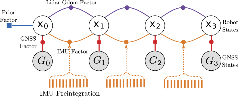
Figure 5: Factor graph structure with preintegrated IMU and lidar factors. GNSS poses are also added as unary factors in the graph.

IV-E1 Prior factor

Prior factors are used to constrain the system with the $\mathtt{{W}}$ frame. Assuming known prior $\tensor[_{\mathtt{W}}]{\mathbf{T}}{{}_{\mathtt{{GNSS}}_{0}}}$, we can anchor our system to the $\mathtt{W}$ frame by computing the residual between the estimated state $\widehat{\boldsymbol{x}}_{0}$, and GNSS based state estimate $\tensor[_{\mathtt{W}}]{\mathbf{T}}{{}_{\mathtt{{GNSS}}_{0}}}$, at $t_{0}$. The residual becomes:

$$\mathbf{r}_{0}=\left(\begin{array}[]{c}\check{\Pi}\left(\widehat{\mathbf{T}}_{0}^{-1}\mathbf{T}_{\mathtt{{GNSS}}_{0}}\right)\\ \widehat{\mathbf{v}}_{0}-[0\;0\;0]^{\mathtt{T}}\\ \widehat{\mathbf{\boldsymbol{\omega}}}_{0}-[0\;0\;0]^{\mathtt{T}}\\ \widehat{\mathbf{b}}_{0}^{a}-\mathbf{b}_{{0}}^{a}\\ \widehat{\mathbf{b}}_{0}^{\omega}-\mathbf{b}_{{0}}^{\omega}\end{array}\right),$$ (15)

where, $\check{\Pi}$ is the lifting operator used to solve the optimization in tangent space according to the “lift-solve-retract” principle presented in [20].

IV-E2 IMU pre-integration factor

We use the standard formulation for IMU measurement pre-integration [20] to create the IMU factor between consecutive nodes of the pose graph. The high frequency pose update (at about 100Hz) is also used by the lidar odometry module. The residual has the form (with a derivation taken from [20]):

$$\mathbf{r}_{{\cal I}_{ij}}=\left[\mathbf{r}^{\mathsf{T}}_{\Delta\mathbf{R}_{ij}},\mathbf{r}^{\mathsf{T}}_{\Delta\mathbf{t}_{ij}},\mathbf{r}^{\mathsf{T}}_{\Delta\mathbf{v}_{ij}},\mathbf{r}_{\mathbf{b}^{a}_{ij}},\mathbf{r}_{\mathbf{b}^{g}_{ij}}\right].$$ (16)

IV-E3 Lidar odometry and between factor

Lidar odometry

For the lidar odometry we register the fused downsampled point cloud directly to local submap using ikd-tree [15] leveraging its computational efficiency when finding correspondences. ICP is performed between corresponding points to infer relative motion, using a motion prior from IMU pre-integration. We register lidar poses at ICP frequency ($\approx$ 2 Hz), so as to used to maintain a smooth local submap. Since we directly register the raw point clouds to the local submap without feature engineering it improves the accuracy of the odometry system in feature-less environments. Also, as we are not specifically doing SLAM, we update the local submap periodically. This helps in managing a small memory footprint unlike maintaining a global map (which would need large memory) required for the lidar odometry.

Between factor formulation

Based on our optimization window we may sample multiple lidar odometry measurements between $t_{i}$ and $t_{j}$. However, to constrain the pose graph with a single between factor within the smoothing window we use the first and the last estimated poses from the lidar odometry module, denoted as, $\widehat{\mathbf{T}}_{i+\epsilon}$ and $\widehat{\mathbf{T}}_{j-\epsilon}$ respectively. Note that we add the term $\epsilon$ to denote the lidar odometry module processing time. Considering $\epsilon\to 0$, the residual has the form:

$$\mathbf{r}_{{\cal L}_{ij}}=\check{\Pi}\left(({\mathbf{T}}_{i}^{-1}{\mathbf{T}}_{j})^{-1}\widehat{\mathbf{T}}_{i}^{-1}\widehat{\mathbf{T}}_{j}\right).$$ (17)

IV-E4 GNSS prior factor

Lidar inertial odometry will drift over time. Hence, to constrain the state estimation over long distances, we add only the $\tensor[_{\mathtt{W}}]{\mathbf{t}}{{}_{\mathtt{{GNSS}}}}$ represented in UTM co-ordinates as a prior on our factor graph formulation if the estimated position covariance is larger than the GNSS position covariance adapted from [13]. Note that our graph formulation will naturally produce state estimates even when no GNSS information is available. Since, we only use the translation components, the residual becomes:

$$\mathbf{r}_{{\cal G}_{i}}=|\tensor[_{\mathtt{W}}]{\mathbf{t}}{{}_{\mathtt{{GNSS}}_{i}}}-\tensor[_{\mathtt{W}}]{\mathbf{t}}{{}_{\mathtt{{\mathtt{{B}}}}_{i}}}|.$$ (18)

For simplicity, we have used constant values for the covariances of IMU pre-integration factor, lidar between factor and GNSS prior factor for our experiments.

V Experimental Results

To demonstrate system performance, we conducted several experiments in real world environments including urban and highway driving scenarios to collect data using two vehicles with the sensor setup illustrated in Fig. 2.

V-A Dataset

All sensing data in our vehicle is synchronized using PTP (Precision Time Protocol). For ground truth (GT) pose estimates, we use data from a GNSS receiver.

We use the following notation to distinguish between different sensor configurations – $\mathbf{L_{n_{l}}I_{n_{i}}G_{n_{g}}}$ (L: Lidar, I: IMU and G: GNSS); with $\mathbf{n_{l}}$, $\mathbf{n_{i}}$ and $\mathbf{n_{g}}$: indicating the corresponding number of sensor.

We collected 5 test sequences which is described in details in Table I. Lossy signal conditions were emulated manually for our experiments by dropping individual sensor signals randomly once for a period of 5-10 seconds in two data logs. For the single modality experiments, we use the $F_{L}$ lidar and its corresponding IMU in both the bus and the truck logs.

Datasets collection details for the experiments
Data	Vehicle	Scenario	Sensor setup	Length ($\mathrm{K}\mathrm{m}$)	Duration ($\mathrm{s}\mathrm{e}\mathrm{c}\mathrm{s}$)	Signal loss
Seq-1	Bus	Urban	${L_{4}I_{4}G_{1}}$	1.643	333.37	Yes
Seq-2†	Bus	Highway	${L_{4}I_{4}G_{1}}$	1.948	168.64	No
Seq-3†	Bus	Highway	${L_{4}I_{4}G_{1}}$	1.577	118.56	No
Seq-4	Truck	Urban	${L_{4}I_{4}G_{1}}$	0.453	78.91	No
Seq-5	Truck	Urban	${L_{4}I_{4}G_{1}}$	1.267	151.37	Yes
†Four front lidars and IMUs are used for this log sequence.

TABLE I:

We demonstrate the lidar fusion method and its results in signal dropout scenario in the supplementary video.

V-B IMU fusion

All the IMUs from the integrated sensor housing (shown in Fig. 2) are oriented along the $\mathtt{{B}}$ frame using the predefined calibration parameters. Due to limited space availability, we only visualize and discuss the results of the fusion of the angular velocity (Y-component) for Seq-1 and confirm that a similar hypothesis holds true for the other IMU signal components in all the sequences. As seen in Fig. 6, the angular velocity components look out-of-phase, since they are not transformed to the $\mathtt{{B}}$ frame. Also, around fifth second in Fig. 6, we observe that there was a signal loss for the $F_{L}$ and $R_{R}$ IMU for around 10 seconds.

After applying the MIMU fusion technique, described in Sec. IV-D, with the correct calibration parameters we get a fused MIMU signal in $\mathtt{{B}}$ frame, which is robust to signal loss as seen in Fig. 7. We also analyzed the fused signal wrt GT and verify the quality of the fusion. The GT IMU signal is logged from the GNSS system in $\mathtt{{B}}$ frame. As seen in Fig. 7 our fused signal for the angular velocity (Y-component) closely corresponds to its respective GT.

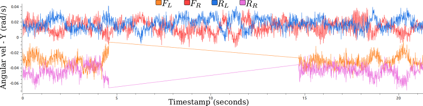
Figure 6: IMU raw signal of angular velocity (Y-component).

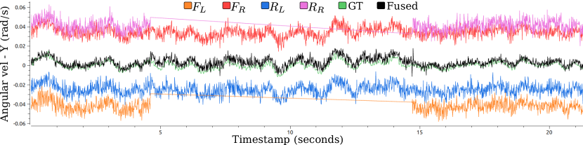
Figure 7: IMU fusion of angular velocity (Y-component).

RMSE of IMU Fusion wrt Ground Truth
Data	Average Fusion		MLE Fusion
	Linear acceleration	Angular velocity	Linear acceleration	Angular velocity
Seq-1	2.868	0.004	1.716	0.003
Seq-2	2.219	0.003	1.814	0.003
Seq-3	2.186	0.003	1.792	0.003
Seq-4	2.041	0.008	1.818	0.007
Seq-5	2.263	0.008	1.820	0.007

TABLE II:

To provide more detailed analysis we summarize our RMSE error for the fused signal wrt the GT signal and compare its performance to a fusion approach based on averaging of the signals in Tab II. For the RMSE, we compared the linear acceleration and the angular velocity components separately as, $\operatorname{RMSE}=\sqrt{\frac{1}{N}\|I_{GT}-\widehat{I}\|^{2}_{F}}$.

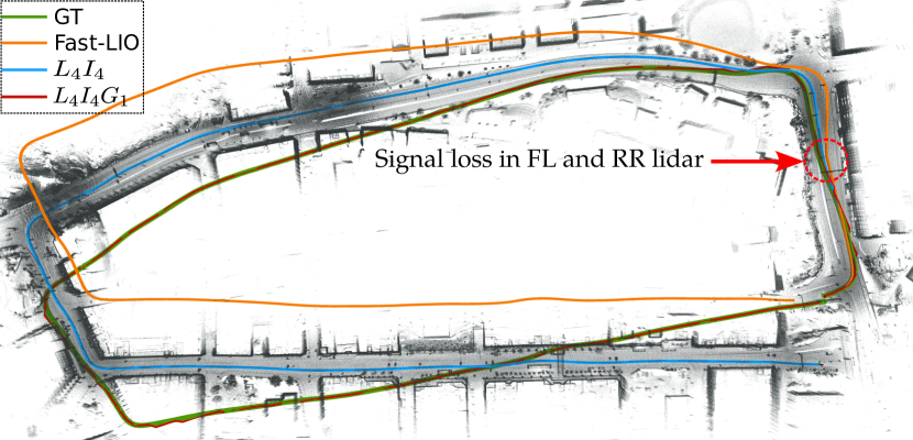
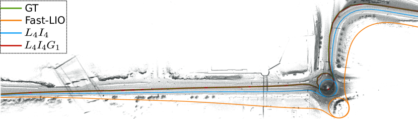
Figure 8: Seq 1: Driving scenario with $F_{L}$ and $R_{R}$ lidar signal loss (Bus)

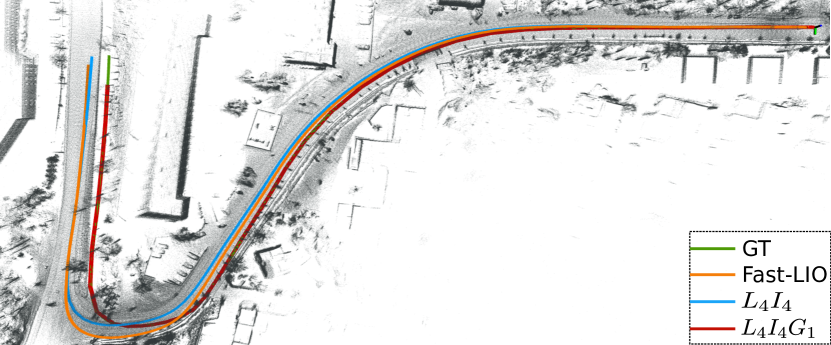
Figure 9: Seq 2: Driving scenario with a roundabout (Bus)

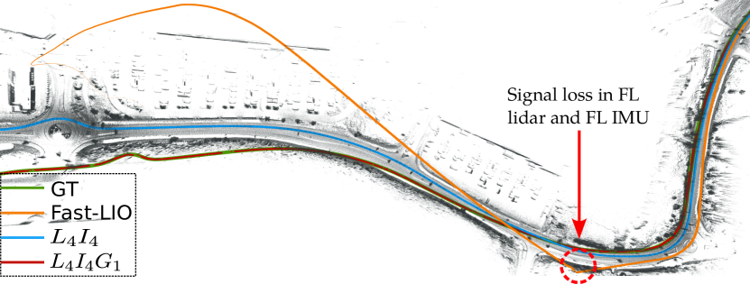
Figure 10: Seq 4: Driving scenario with long turning radius (Truck)

Figure 11: Seq 5: Driving scenario with $F_{L}$ lidar and IMU signal loss (Truck)

V-C State Estimation

The relative pose error (RPE) and absolute pose error (APE) metrics are used to evaluate the local and global consistency respectively of the estimated poses. RPE compares the relative pose along the estimated and the reference trajectory between two timestamps $t_{i}$ and $t_{j}$, using the relative transform over a specific distance traveled (10 $\mathrm{m}$) as,

$$\operatorname{RPE}_{i,j}=({\mathbf{T}}_{GT_{i}}^{-1}{\mathbf{T}}_{GT_{j}})^{-1}(\widehat{{\mathbf{T}}}{{}_{i}^{-1}}\widehat{{\mathbf{T}}}{{}_{j}}).$$ (19)

APE is based on the absolute relative pose difference between two poses ${\mathbf{T}}{{}_{GT_{i}}}$ and $\widehat{{\mathbf{T}}}{{}_{i}}$ at timestamp $t_{i}$ and is compared for the whole trajectory of $N$ timestamps as,

$$\operatorname{APE}_{N}=\sqrt{\frac{1}{N}\sum_{i=1}^{N}\|{\mathbf{T}}{{}_{GT_{i}}^{-1}}\widehat{\mathbf{T}}{{}_{i}}-I_{4\times 4}\|^{2}_{F}}.$$ (20)

In our experiments to demonstrate the performance improvement of using multiple sensors versus a single sensor when signal loss occurs we used the $L_{4}I_{4}$ configuration, described in Sec. V-A. To illustrate the reduction in drift when additionally fusing GNSS, we used the $L_{4}I_{4}G_{1}$ configuration.

As seen in Fig. 6, signal loss for few seconds occurs in Seq-1 (Fig. 11). Fast-LIO2 drifts quickly at that point — but maintains consistency in the rest of the trajectory. Meanwhile, the $L_{4}I_{4}$ configuration handles this situation seamlessly using the other available sensor signals.

In the highway scenario of Seq-2 (Fig. 11), we see that again $L_{4}I_{4}$ configuration outperforms Fast-LIO2 as there are very few environmental structures. Hence, expanding the lidar field-of-view using $L_{4}I_{4}$ gives more constraints for the ICP matching, outperforming Fast-LIO2.

In Seq-5 (Fig. 11), we manually induced a data drop in the $F_{L}$ lidar and IMU for 8 seconds. Fast-LIO2 again fails to recover from the situation, whereas, $L_{4}I_{4}$ configuration performs well again.

Pose Error – RPE (Translation[$\mathrm{m}\text{/}$], Rotation [$\mathrm{\SIUnitSymbolDegree}\text{/}$]) / APE
Data	$\mathbf{L_{4}I_{4}}$	$\mathbf{L_{4}I_{4}G_{1}}$	$\mathbf{Fast-LIO2}\textsuperscript{\textdagger}$
Seq-1	0.676, 1.248 / 4.992	0.115, 1.719 / 3.574	0.977, 1.458 / 11.137
Seq-2	0.419, 0.264 / 5.376	0.158, 0.804 / 4.342	0.673, 0.458 / 24.422
Seq-3	0.361, 0.228 / 3.479	0.221, 0.655 / 2.268	0.421, 0.298 / 13.770
Seq-4	0.835, 0.471 / 1.446	0.106, 0.719 / 0.785	0.824, 0.457 / 0.9840
Seq-5	1.265, 0.454 / 9.556	0.605, 1.479 / 1.645	26.815, 2.238 / 4613.7
†Fast-LIO2 $={L_{1}I_{1}}$ configuration.

TABLE III:

Table III, show RPE and APE metrics for each sequence with Fast-LIO2 acting as the baseline. In all the scenarios, the $L_{4}I_{4}G_{1}$ configuration outperform the other methods, as GNSS pose priors are added seamlessly in a graph based optimization, which constrains the pose drift but suffers from discontinuities; thus for visualization of the lidar map we use the $L_{4}I_{4}$ lidar odometry frame. In most of the scenarios the RPE and APE for $L_{4}I_{4}$ configuration is less than Fast-LIO2, since it encompasses a wider field-of-view with more matching constraints for ICP. However, in Seq-4 (Fig. 11) Fast-LIO2 is performing slightly better as the vehicle is driven in a structure rich environment with no signal dropouts. For Seq-3 results please check our supplementary video.

VI Conclusion

We have presented a method for multi-lidar and MIMU state estimation in a factor graph optimization framework and additionally demonstrated the use of GNSS priors. The proposed method produces comparable performance to a state-of-the-art lidar-inertial odometry system (Fast-LIO2) but outperforms it when there are signal dropouts with an average improvement of 61% in relative translation and 42% in relative rotational error. For future work we aim to introduce radar as an additional modality to discard dynamic environmental points for improving the odometry estimate.

VII Acknowledgements

This research has been jointly funded by the Swedish Foundation for Strategic Research (SSF) and Scania. The authors would like to thank Ludvig af Klinteberg for his valuable comments which improved the manuscript and Goksan Isil for help with experimental data creation.

References

- [1] X. Zuo, P. Geneva, W. Lee, Y. Liu, and G. Huang, “LIC-Fusion: LiDAR-inertial-camera odometry,” in IEEE/RSJ International Conference on Intelligent Robots and Systems, 2019, pp. 5848–5854.
- [2] T. Shan, B. Englot, C. Ratti, and D. Rus, “LVI-SAM: Tightly-coupled lidar-visual-inertial odometry via smoothing and mapping,” in IEEE International Conference on Robotics and Automation, 2021, pp. 5692–5698.
- [3] D. Wisth, M. Camurri, and M. Fallon, “VILENS: Visual, inertial, lidar, and leg odometry for all-terrain legged robots,” IEEE Transactions on Robotics, pp. 1–18, 2022.
- [4] P. Sun, H. Kretzschmar, X. Dotiwalla, A. Chouard, V. Patnaik, P. Tsui, J. Guo, Y. Zhou, Y. Chai, B. Caine, et al., “Scalability in perception for autonomous driving: Waymo open dataset,” in IEEE Conference on Computer Vision and Pattern Recognition, 2020, pp. 2446–2454.
- [5] J. Geyer, Y. Kassahun, M. Mahmudi, X. Ricou, R. Durgesh, A. S. Chung, L. Hauswald, V. H. Pham, M. Mühlegg, S. Dorn, T. Fernandez, M. Jänicke, S. Mirashi, C. Savani, M. Sturm, O. Vorobiov, M. Oelker, S. Garreis, and P. Schuberth, “A2D2: Audi Autonomous Driving Dataset,” https://www.a2d2.audi, 2020.
- [6] M. Palieri, B. Morrell, A. Thakur, K. Ebadi, J. Nash, A. Chatterjee, C. Kanellakis, L. Carlone, C. Guaragnella, and A. Agha-Mohammadi, “Locus: A multi-sensor lidar-centric solution for high-precision odometry and 3d mapping in real-time,” IEEE Robotics and Automation Letters, vol. 6, no. 2, pp. 421–428, 2020.
- [7] J. Jiao, H. Ye, Y. Zhu, and M. Liu, “Robust odometry and mapping for multi-lidar systems with online extrinsic calibration,” IEEE Transactions on Robotics, vol. 38, no. 1, pp. 351–371, 2021.
- [8] I. Skog, J. O. Nilsson, P. Händel, and A. Nehorai, “Inertial sensor arrays, maximum likelihood, and cramér–rao bound,” IEEE Transactions on Signal Processing, vol. 64, no. 16, pp. 4218–4227, 2016.
- [9] M. Faizullin and G. Ferrer, “Best axes composition: Multiple gyroscopes imu sensor fusion to reduce systematic error,” in IEEE European Conference on Mobile Robots, 2021, pp. 1–7.
- [10] J. Zhang and S. Singh, “Low-drift and real-time lidar odometry and mapping,” Autonomous Robots, vol. 41, no. 2, pp. 401–416, Feb. 2017.
- [11] A. Segal, D. Haehnel, and S. Thrun, “Generalized-ICP,” in Robotics: science and systems, vol. 2, no. 4. Seattle, WA, 2009, p. 435.
- [12] T. Shan and B. Englot, “LeGO-LOAM: Lightweight and ground-optimized lidar odometry and mapping on variable terrain,” in IEEE/RSJ International Conference on Intelligent Robots and Systems, 2018, pp. 4758–4765.
- [13] T. Shan, B. Englot, D. Meyers, W. Wang, C. Ratti, and D. Rus, “Lio-sam: Tightly-coupled lidar inertial odometry via smoothing and mapping,” in IEEE/RSJ International Conference on Intelligent Robots and Systems, 2020, pp. 5135–5142.
- [14] J. Engel, T. Schöps, and D. Cremers, “LSD-SLAM: Large-scale direct monocular slam,” in European Conference on computer vision, 2014, pp. 834–849.
- [15] W. Xu, Y. Cai, D. He, J. Lin, and F. Zhang, “FAST-LIO2: Fast direct lidar-inertial odometry,” IEEE Transactions on Robotics, vol. 38, no. 4, pp. 2053–2073, 2022.
- [16] C. Bai, T. Xiao, Y. Chen, H. Wang, F. Zhang, and X. Gao, “Faster-LIO: Lightweight tightly coupled lidar-inertial odometry using parallel sparse incremental voxels,” IEEE Robotics and Automation Letters, vol. 7, no. 2, pp. 4861–4868, 2022.
- [17] P. Furgale, “Representing robot pose: The good, the bad, and the ugly,” in Workshop on Lessons Learned from Building Complex Systems, IEEE International Conference on Robotics and Automation, 2014.
- [18] M. Pedley, “Tilt sensing using a three-axis accelerometer,” Freescale semiconductor application note, vol. 1, pp. 2012–2013, 2013.
- [19] D. W. Allan, “Statistics of atomic frequency standards,” Proceedings of the IEEE, vol. 54, no. 2, pp. 221–230, 1966.
- [20] C. Forster, L. Carlone, F. Dellaert, and D. Scaramuzza, “On-manifold preintegration for real-time visual-inertial odometry,” IEEE Transactions on Robotics, vol. 33, no. 1, pp. 1–21, 2017.
- [21] L. Kavan and J. Žára, “Spherical blend skinning: a real-time deformation of articulated models,” in Symposium on Interactive 3D graphics and games, 2005, pp. 9–16.
- [22] F. Dellaert and M. Kaess, “Factor graphs for robot perception,” Foundations and Trends in Robotics, vol. 6, pp. 1–139, Aug. 2017.