Geometrical and physical interpretation of the Levi-Civita spacetime
in terms of the Komar mass density

Abstract

We revisit the interpretation of the cylindrically symmetric, static vacuum Levi-Civita metric, known in either Weyl, Einstein-Rosen, or Kasner-like coordinates. Despite the infinite axis source, we achieve a rigurous derivation of its Komar mass density through a compactification and subsequent blowing up of the compactification radius. The Komar mass density turns out coordinate system dependent, the timelike Killing vector (in the absence of a preferred normalization) being adopted to the coordinate time in each of the available systems. We show that among all possibilities, the Komar mass density $\mu_{K}$ calculated in the Einstein-Rosen frame, when employed as the metric parameter, has a number of advantages over other parametrizations. First it eliminates previous double coverages of the parameter space. It vanishes in flat spacetime and when small, it corresponds to the mass density of an infinite string. It characterizes the Kretschmann scalar in the simplest possible way (no double coverage of the parameter space, neither a multivalued function, as with other parameters). After a comprehensive analysis of the local and global geometry (including a study of the singularity on the axis, based on the Królak and Tipler criteria, and refuting earlier related claims), we proceed with the physical interpretation of the Levi-Civita spacetime. First we show that the Newtonian gravitational force is attractive and its magnitude increases monotonically with all positive $\mu_{K}$, asymptoting to $R^{-1}$ (with $R$ the proper distance in the "radial" direction). Second, we reveal that the magnitude of the tidal force between nearby timelike geodesics (hence gravity in the Einsteinian sense) attains a maximum at $\mu_{K}=1/2$ and then decreases asymptotically to zero. Hence, from a physical point of view the Komar mass density of the Levi-Civita spacetime encompasses two contributions: Newtonian gravity and acceleration effects. An increase in $\mu_{K}$ strengthens Newtonian gravity but also drags the field lines increasingly parallel, eventually transforming Newtonian gravity through the equivalence principle into a pure acceleration field (with acceleration $R^{-1}$) and the Levi-Civita spacetime into a flat Rindler-like spacetime. In a geometric picture the increase of $\mu_{K}$ from zero to $\infty$ deforms the $t=$const, $z=$const planar sections of the Levi-Civita spacetime into ever deepening funnels, eventually degenerating into cylindrical topology.

I Introduction

Gravitational waves were predicted in the early days of general relativity, as wavelike perturbations of flat spacetime propagating with the speed of light GWfirst , but only in recent years they were detected (see the catalog of 90 gravitational waves GWTC3 by the LIGO Scientific, Virgo and KAGRA Collaborations). As the existence of spherically symmetric gravitational waves in vacuum is forbidden by the Jebsen-Birkhoff theorem, the next simplest geometry would be cylindrically symmetric. Cylindrical symmetry also provides the next simplest setup (after spherical symmetry) for discussing both mathematical and physical aspects of spacetimes with localized sources, emerging as solutions of the Einstein equation and it is also a precursor for studying axial symmetry.

Unlike in the spherically symmetric case, the cylindrically symmetric vacuum is not unique. The Einstein-Rosen cylindrically symmetric vacuum solutions include wavelike behaviors, allowing for both standing wave and approximate progressive wave solutions, discovered analytically in the very early days of general relativity by Einstein and Rosen EinsteinRosen . Later both solitonic waves BelinskiiZakharov and impulsive wave solutions Carmeli , HerreraSantos were identified in this class.

The canonical quantization of cylindrically symmetric gravitational waves by Kuchař was the earliest example of the midisuperspace approach KucharCylindric , which encompasses a much richer structure than previous minisuperspace quantizations of the Friedmann and mixmaster universes (by DeWitt DeWitt and Misner Misner1 ; Misner2 ; Misner3 , respectively). Due to a fair compromise between the simplicity induced by degrees of freedom frozen by symmetry assumptions on the one hand and the full complexity of the gravitational degrees of freedom on the other hand, cylindrical gravitational waves provide an ideal testbed for comparing quantization approaches.

In a strong field a fast changing gravitational wave can be separated from a slowly changing background in the geometrical optics (high frequency) approximation, as discussed thoroughly by Isaacson Isaacson1 ; Isaacson2 . The key concept here is that the curvature radius of the background ought to be much larger than the wavelength. A cylindrically symmetric, static background for the cylindrical gravitational waves, which could represent such a strong field, is the Levi-Civita spacetime Levi-Civita , the static limit of the Einstein-Rosen class.

This static vacuum solution was derived by Levi-Civita in 1919 Levi-Civita , with the intent to characterize the gravitational vacuum outside a cylindrically symmetric source. Generalizations of the static Levi-Civita solution beyond vacuum are also known. The exterior of a radiating cylinder was discussed in Ref. Rao . This radiating Levi-Civita spacetime contains a null dust, in this sense being similar to the spherically symmetric Vaidya metric. Electrovacuum generalisations also emerged, including the inclusion of axial or longitudinal magnetic fields by Bonnor Bonnor and radial electric field by Raychaudhuri Raychaudhuri .

The Levi-Civita static and Einstein-Rosen wavelike solutions with their possible sources have been studied in Refs. Marder , Thorne , Bonnor79 , GriffithsP . However, even for the static vacuum case certain aspects related to its physical interpretation remain elusive. It is the purpose of this paper to revisit the static Levi-Civita spacetime, sheding light on these key properties, both from geometric and physical viewpoints.

The Levi-Civita metric was discovered and has been often discussed in the Weyl form, suitable for static and axially symmetric scenarios. While a small positive metric parameter $\lambda$ has the convenient interpretation of the linear mass density along the symmetry axis of the cylinder (it agrees with it in a first order expansion in $\lambda$ Marder ), the interpretation seems to break down at $\lambda=1/4$, above which the Kretschmann scalar decreases with increasing $\lambda$ GautreauHoffman , Bonnorlambda4 . Furthermore, there is no unique flat spacetime limit, the Levi-Civita spacetime becoming flat for the quartet of values $\lambda=0$, $1/2$ and $\lambda\rightarrow\pm\infty$ GriffithsP . Clearly, the metric parameter $\lambda$ lacks a crystal clear physical meaning, being by far no proper analogue for the mass parameter of the Schwarzschild spacetime.

Einstein-Rosen waves are naturally described in another coordinate system, suitable for cylindrical symmetry. This is the particular nonrotating limit of the Jordan-Ehlers-Kundt-Kompaneets coordinates Bini . The Weyl and Einstein-Rosen metric forms are related through the analytical continuation $t\rightarrow i\widehat{z}$, $z\rightarrow i\widehat{t}$ (with $t$ and $z$ the temporal and axial Einstein-Rosen coordinates, their Weyl counterparts carrying a hat), generating an axially symmetric stationary metric in the Weyl form from a cylindrically symmetric metric. The Levi-Civita spacetime, being both static and cylindrically symmetric, in addition allows for a real coordinate transformation between these two forms Marder , Thorne .

In Sec. 2 we summarize the preliminaries necessary for our discussion. We start from the Einstein-Rosen form (also known as canonical, derived in Appendix A from a more general standard form) of a cylindrically symmetric metric with vorticity-free Killing vectors and orthogonally transitive group action, to specify the metric functions leading to the Levi-Civita metric. We present the transformation between its Weyl and Einstein-Rosen forms explicitly, as we were unable to locate it elsewhere in the literature. The Levi-Civita metric in the Einstein-Rosen form closely mimics the properties established in Weyl coordinates. For a quartet of values of the metric parameter $\sigma=0$, $1$, and $\pm\infty$ the curvature disappears. For small negative values of the parameter $\sigma$ the interpretation of a (Newtonian) gravitational field generated by a homogeneous cylinder holds. For other values however, it breaks down, including a range of parameter values with repulsive gravity. For both the Weyl and the Einstein-Rosen forms the properties of the respective parameters suggest a double coverage of the available configurations. At the end of Sec. 2., preparing for the next section, we summarize the essentials of the Komar superpotential and charges.

Sec. 3. contains a rigorous derivation of the Komar mass density $\mu_{K}$ of the Levi-Civita spacetime in the Einstein-Rosen coordinates. This is achieved despite the infinite source along the axis, through a compactification and subsequent blowing up of the compactification radius. Next we propose $\mu_{K}$ as yet another parameter of the Levi-Civita metric, which has the advantage to eliminate the double coverage encountered before. The metric is flat for $\mu_{K}=0$ and the Komar mass density has the interpretation of linear mass density on the symmetry axis up to $\mu_{K}=1$. At $\mu_{K}\rightarrow\infty$ the metric is flat again, this time in uniformly accelerated Rindler coordinates. As with increasing $\mu_{K}$ the Levi-Civita metric approaches the Rindler limit, we conjecture that beside mass and Newtonian gravitational energy, the Komar mass density also encompasses acceleration contributions. We illustrate this point in Appendix B showing that the Rindler metric also generates a nonvanishing Komar mass density. At the end of the section we discuss the C-energy Thorne , Bini of the Levi-Civita metric, showing that it increases monotonically with $\mu_{K}\geq 0$. When reexpressing it in terms of the Komar mass density calculated in the Weyl coordinates, $\left(\mu_{K}\right)_{\mathrm{Weyl}}=$ $\lambda$, this property is lost, supporting the claim that $\mu_{K}$ is the best available metric parameter.

In Sec. 4. we analyze the behaviour of the curvature invariants parametrized by the Komar mass density, in terms of the proper radial distance. We find a maximum of the Kretschmann scalar $\mathcal{K}$ at $\mu_{K}=1$ and the rest of the scalars expressed in terms of $\mathcal{K}$ and $\mu_{K}$ alone. The increase and subsequent decrease of the Kretschmann curvature with $\mu_{K}$ is counterintuitive, undermining the interpretation of $\mu_{K}$ as mass density for $\mu_{K}>1$. Despite the metric apparently diverging for $\mu_{K}\rightarrow\infty$, the curvature invariants vanish there (which comes as no surprise as $\mu_{K}\rightarrow\infty$ corresponds to $\lambda=1/2$, where the Levi-Civita spacetime is known to be flat). This emerging flatness is manifest in the well-known Kasner-like coordinate system GriffithsP , which is regular for both flat limits and explores a redefined time together with the proper radial distance as new coordinates. We rewrite the Kasner parameters in terms of the Komar mass density. For $\mu_{K}\rightarrow\infty$ the metric emerges flat in accelerated Rindler coordinates.

Recently Ref. Ahmed presented a new cylindrically symmetric vacuum spacetime, claiming that the axis is a null geodesically incomplete soft singularity both in the sense of Królak Krolak and of Tipler Tipler . The C-energy density measured by an observer was also computed, the algebraic type shown to be Petrov type D and the geodesic deviation of timelike geodesics synchronized by the proper time. In Appendix C we prove that the metric of Ref. Ahmed  is nothing but the particular case of the Levi-Civita metric for $\mu_{K}=1$. By taking the particular case of the curvature invariants we correct the respective expressions of Ref. Ahmed . Then in the last subsection of Sec. 4. we analyse the nature of the singularity on the symmetry axis and prove that the radial null geodesics in the Levi-Civita spacetime obey both the Królak and the Tipler strong singularity conditions, irrespective of the value of $\mu_{K}$ (hence we disprove the claim of Ref. Ahmed , according to which the singularity on the axis ought to be soft). The technicalities of the proof are deferred to Appendix D.

In Sec. 5. we proceed with the physical interpretation of the Levi-Civita spacetime for generic Komar mass densities by considering the acceleration necessary to keep a stationary observer in orbit at fixed proper distance from the axis. We show that for positive $\mu_{K}$ the gravitational acceleration is attractive and increases monotonically with $\mu_{K}$, asymptoting to a constant value. Hence, despite increasing $\mu_{K}$, Newtonian gravitational attraction cannot increase above a certain limit. Then, we study the magnitude of the tidal forces, showing that the geodesic deviation also exhibits a maximum, this time at $\mu_{K}=1/2$.

We summarize the geometric and physical characterization of the Levi-Civita metric in the discussion presented as Sec. 6.

Throughout the paper we use units $G=1=c$.

II Preliminaries

In this section we summarize the main ingredients necessary for a subsequent thorough investigation of the Levi-Civita spacetime.

II.1 Einstein-Rosen and Weyl forms of the Levi-Civita spacetime

The Einstein–Rosen, or canonical form of the line element of a generic vacuum cylindrically symmetric spacetime with vorticity-free Killing vectors and orthogonally transitive group action (dubbed as whole-cylinder symmetry by Thorne Thorne ), is (for a derivation see Appendix A)

$$\mathrm{d}s^{2}=e^{2\left(K-U\right)}\left(-\mathrm{d}t^{2}+\mathrm{d}r^{2}\right)+e^{-2U}r^{2}\mathrm{d}\varphi^{2}+e^{2U}\mathrm{d}z^{2}\leavevmode\nobreak\ ,$$ (1)

with $K$ and $U$ functions of the coordinates $\left(t,r\right)$. Here all coordinates are dimensionless. For $K=0=U$ or $K=U=\ln r$ the line element (1) degenerates into the flat metric.

These symmetries and the vacuum condition do not guarantee a unique solution of the Einstein equations. Indeed, they allow for various type of Einstein–Rosen waves EinsteinRosen beside the static Levi-Civita solution. The latter emerges for

$$U=\sigma\ln r\leavevmode\nobreak\ ,\quad K=\sigma^{2}\ln r\leavevmode\nobreak\ ,$$ (2)

giving

$$\mathrm{d}s^{2}=r^{2\sigma\left(\sigma-1\right)}\left(-\mathrm{d}t^{2}+\mathrm{d}r^{2}\right)+r^{2\left(1-\sigma\right)}\mathrm{d}\varphi^{2}+r^{2\sigma}\mathrm{d}z^{2}\leavevmode\nobreak\ ,$$ (3)

with a constant $\sigma\in\mathbb{R}$.

Levi-Civita considered a different line element in the axially symmetric and static Weyl form:

$$\mathrm{d}s^{2}=-\widehat{r}^{4\lambda}\mathrm{d}\widehat{t}^{2}+\widehat{r}^{4\lambda\left(2\lambda-1\right)}\left(\mathrm{d}\widehat{r}^{2}+\mathrm{d}\widehat{z}^{2}\right)+\widehat{r}^{2\left(1-2\lambda\right)}\mathrm{d}\widehat{\varphi}^{2}\leavevmode\nobreak\ ,$$ (4)

with $\lambda\in\mathbb{R}$. Both metrics (3) and (4) are static and cylindrically symmetric, hence they ought to be related. Indeed, they transform into each other through the analytical continuation $t\rightarrow i\widehat{z}$, $z\rightarrow i\widehat{t}$ ExSol .

An explicit coordinate transformation

$$t =\left(\sigma-1\right)^{-2p_{0}}\widehat{t}\leavevmode\nobreak\ ,$$

$$r =\left(\sigma-1\right)^{2/\left(\sigma^{2}-\sigma+1\right)}\widehat{r}^{1/\left(\sigma-1\right)^{2}}\leavevmode\nobreak\ ,$$

$$\varphi =\left(\sigma-1\right)^{-2p_{+}}\widehat{\varphi}\leavevmode\nobreak\ ,$$

$$z =\left(\sigma-1\right)^{-2p_{-}}\widehat{z}\leavevmode\nobreak\ ,$$ (5)

with

$$p_{0}=\frac{\sigma\left(\sigma-1\right)}{\sigma^{2}\!-\!\sigma\!+\!1}\leavevmode\nobreak\ ,\leavevmode\nobreak\ \leavevmode\nobreak\ p_{+}=\frac{1-\sigma}{\sigma^{2}\!-\!\sigma\!+\!1}\leavevmode\nobreak\ ,\leavevmode\nobreak\ \leavevmode\nobreak\ p_{-}=\frac{\sigma}{\sigma^{2}\!-\!\sigma\!+\!1}$$ (6)

can also be constructed, where

$$\sigma=\frac{2\lambda}{2\lambda-1}\leavevmode\nobreak\ .$$ (7)

The coordinate transformation (singular for $\sigma=1$ or $\lambda=1/2$) is obtained by transforming both metrics into a Kasner-like form. In the case of a small parameter $\lambda\approx-\sigma/2$ (thus $\sigma$ also small), (5) is close to the identity transformation and reduces to it for $\sigma\rightarrow 0$.

The line elements (3) and (4) are thus locally isometric. The isometry fails to be global if both $\varphi$ and $\widehat{\varphi}$ are angular coordinates with period $2\pi$. Indeed, if the Einstein-Rosen azimuthal angle is periodic with $2\pi$, the period of the Weyl azimuthal coordinate becomes $2\pi\left(\sigma-1\right)^{2p_{+}}$.

For $0\leq\lambda\ll 1$ (thus $\sigma\approx-2\lambda$ in the small negative value range) the parameter $\lambda$ has the interpretation of the constant mass per unit length of a static cylinder with negligible internal pressure Thorne . Indeed, the cylindrically symmetric Laplace equation

$$\nabla^{2}\phi_{N}=\frac{1}{r}\frac{d}{dr}\left(r\frac{d\phi_{N}}{dr}\right)=0$$ (8)

for the Newtonian potential is solved as $\phi_{N}=2m\ln r$ (with $m$ an integration constant and another irrelevant integration constant dropped). Defining the mass $M=\int_{V}\rho dV$ of a cylindrical volume $V$ (containing a distributional source $\rho$ on the axis) through the Poisson equation $\nabla^{2}\phi_{N}=4\pi\rho$ leads to

$$M=\frac{1}{4\pi}\int_{\partial V}\mathbf{\nabla}\phi_{N}\cdot d\mathbf{A}=m\int dz\mathbf{\leavevmode\nobreak\ ,}$$ (9)

where $d\mathbf{A}$ is the outward directed normal of the boundary $\partial V$ of the cylinder (however as $\mathbf{\nabla}\phi_{N}=(2m/r)\mathbf{e}_{r}$, only the cylindrical surface contributes). Hence, the constant $m$ is precisely the mass density along the $z$-axis. In the stationary, weak field and slow motion limit $g_{00}\approx-1-2\phi_{N}=-1-4m\ln r$. On the other hand, the Levi-Civita metric in Einstein-Rosen coordinates has $g_{00}=-r^{2\sigma\left(\sigma-1\right)}=-\exp\left[2\sigma\left(\sigma-1\right)\ln r\right]$, which for small $\sigma$ approximates as $g_{00}\approx-1-2\sigma\left(\sigma-1\right)\ln r\approx-1+2\sigma\ln r\approx-1-4\lambda\ln r$, confirming the interpretation $\lambda\approx m$, when small.

In deriving the solution (2) a constant of integration was supressed through the requirement to recover the Minkowski metric in cylindrical coordinates when $\lambda=0$ (hence $\sigma=0$). For $\sigma=1$ [hence $\lambda\rightarrow\pm\infty$, due to Eq. (7)] the metric is also flat (although some of the metric coefficients diverge, other vanish). Clearly, the interpretation of $\lambda$ as mass per length is unsuitable for its whole range. In fact there is a duality in the ranges of either parameters $\lambda$ or $\sigma$, corresponding to an interchange of the coordinates $z$ and $\varphi$ GriffithsP . This duality appears as an unnecessary redundancy in either of the parametrizations.

Moreover, the metric (3) diverges for $\sigma\rightarrow\pm\infty$. In this case, however it can be transformed to the flat metric perceived by an accelerated observer, the Rindler metric. This is exactly the flatness of the Levi-Civita metric in the Weyl form emerging for $\lambda=1/2$ GriffithsP , see Eq. (7).

II.2 The Komar superpotential and charges

We consider a vector field $\xi$ and corresponding $1$-form $\bm{\xi}$ on a four dimensional Lorentzian spacetime $M$. Its Komar superpotential $2$-form Komar

$$\mathbf{U}_{\xi}=\ast\mathrm{d}\bm{\xi}=\frac{1}{2}\left(\nabla^{i}\xi^{j}-\nabla^{j}\xi^{i}\right)\sqrt{\mathfrak{g}}\left(\mathrm{d}^{2}x\right)_{ij}\leavevmode\nobreak\$$ (10)

(where $\mathfrak{g}=\left|\det g_{ij}\right|$ and $\left(\mathrm{d}^{2}x\right)_{ij}=\frac{1}{2}\epsilon_{ijkl}\mathrm{d}x^{k}\wedge\mathrm{d}x^{l}$) is defined through the Hodge dual

$$\ast A=\frac{1}{4}A^{ij}\epsilon_{ijkl}\sqrt{\mathfrak{g}}\mathrm{d}x^{k}\wedge\mathrm{d}x^{l}$$ (11)

of the $2$-form $A=\mathrm{d}\bm{\xi}$, with $\mathrm{d}$ the exterior derivative.

Then the current

$$\mathbf{S}_{\xi}=\mathrm{d}\mathbf{U}_{\xi}=\nabla_{j}\left(\nabla^{i}\xi^{j}-\nabla^{j}\xi^{i}\right)\sqrt{\mathfrak{g}}\left(\mathrm{d}^{3}x\right)_{i}\leavevmode\nobreak\$$ (12)

(with $\left(\mathrm{d}^{3}x\right)_{i}=\frac{1}{6}\epsilon_{ijkl}\mathrm{d}x^{j}\wedge\mathrm{d}x^{k}\wedge\mathrm{d}x^{l}$) is identically conserved. This also emerges as the Noether current of the Einstein-Hilbert action, associated to diffeomorphism invariance FF .

When $\xi$ is a Killing vector field (hence $0=\nabla_{i}\xi_{j}+\nabla_{j}\xi_{i}$), from the cyclic identity of the curvature tensor the relation

$$R_{\ ijk}^{l}\xi_{l}=\nabla_{i}\nabla_{j}\xi_{k}$$ (13)

emerges, which renders $\mathbf{S}_{\xi}$ into

$$\mathbf{S}_{\xi} =2R_{\ j}^{i}\xi^{j}\sqrt{\mathfrak{g}}\left(\mathrm{d}^{3}x\right)_{i}$$

$$=16\pi\left(T_{\ j}^{i}-\frac{1}{2}T\delta_{j}^{i}\right)\xi^{j}\sqrt{\mathfrak{g}}\left(\mathrm{d}^{3}x\right)_{i}\leavevmode\nobreak\ .$$ (14)

In the last step we employed the Einstein equations. Hence in vacuum the Komar superpotential of a Killing field is a closed 2-form.

If a closed set $\mathcal{C}\subseteq M$ encompasses all sources (including four-dimensional extended sources, two-dimensional strings, one dimensional point sourses, singularities, topological defects), then for a closed $2$-surface $\mathcal{S}\subseteq M\setminus\mathcal{C}$ the Komar charge

$$Q_{\xi}\left(\mathcal{S}\right)=\int_{\mathcal{S}}\mathbf{U}_{\xi}$$ (15)

depends on the homology class of $\mathcal{S}$ only. Then every pair of closed $2$-surfaces $\mathcal{S}$ and $\mathcal{S}^{\prime}$ encompassing $\mathcal{C}$ are homologous to each other, e.g. there is a $3$-surface $N\subseteq M\setminus\mathcal{C}$ such that $\partial N=\mathcal{S}-\mathcal{S}^{\prime}$. Stokes’ theorem then gives

$$Q_{\xi}\left(\mathcal{S}\right)-Q_{\xi}\left(\mathcal{S}^{\prime}\right)=\int_{\partial N}\mathbf{U}_{\xi}=\int_{N}\mathrm{d}\mathbf{U}_{\xi}=0\leavevmode\nobreak\ ,$$ (16)

which shows that the Komar charge is conserved. If $\mathcal{S}$ and $\mathcal{S}^{\prime}$ are both spacelike and $N$ timelike, this corresponds to a conservation law in the sense that $Q_{\xi}$ takes the same value at all times.

When $\xi$ is a timelike Killing vector field, then

$$m_{K}=-\frac{1}{8\pi}Q_{\xi}\left(\mathcal{S}\right)=-\frac{1}{8\pi}\int_{\mathcal{S}}\mathbf{U}_{\xi}$$ (17)

is the Komar mass of the spacetime. The integral $m_{K}$ is however ambigous to a constant factor, since $a\xi$ is an equally valid Killing vector (here $a\in\mathbb{R}^{+}$). The ambiguity can be removed when a preferred normalization of the timelike Killing vector is available (like $\xi\cdot\xi\rightarrow-1$ at asymptotic infinity).

III A new parametrization of the Levi-Civita metric

In this section we first introduce a mathematically sound construction for defining the Komar mass density $\mu_{K}$ for the Levi-Civita spacetime in the Einstein-Rosen form, and will explore it as an alternative metric parameter. One of its main advantages over the previously used parameters $\lambda$ or $\sigma$ is that it eliminates the double coverage appearing in either of them. The $C$-energy of the spacetime provides additional support for considering $\mu_{K}$ as a natural parameter of the Levi-Civita spacetime.

III.1 Komar mass density for the Levi-Civita spacetime

The static, cylindrically symmetric Levi-Civita spacetime has a three dimensional Killing algebra with a timelike Killing vector, a spacelike axial Killing vector and a translational Killing vector along the $z$-axis (which, being singular, is removed from the manifold). In the coordinates (3) the squared length of the timelike Killing vector field $\xi=a\partial_{t}$ (with $a$ a constant) is $\xi\cdot\xi=-a^{2}r^{2\sigma\left(\sigma-1\right)}$. Aside from special values of the parameter $\sigma=0,1$ where the metric is flat, this Killing vector field cannot be normalized either at infinity or the axis, hence we adopt the simplest choice $a=1$ (adapting the temporal Killing vector field to the coordinate time).

The singularity on the axis $r=0$ extends to infinity, thus it is impossible to wrap it in a closed $2$-surface, as required for the evaluation of the Komar charge. Despite this in what follows we describe a procedure allowing for the definition of the density $\mu_{K}$ of the Komar mass along the $z$-axis.

The key step is to compactify the $z$ direction as $z=l\alpha$, where $l$ is a length scale and $\alpha$ an angle parameter with periodicity $2\pi$. The line element (3) becomes

$$\mathrm{d}s^{2}=r^{2\sigma\left(\sigma-1\right)}\left(-\mathrm{d}t^{2}+\mathrm{d}r^{2}\right)+r^{2\left(1-\sigma\right)}\mathrm{d}\varphi^{2}+r^{2\sigma}l^{2}\mathrm{d}\alpha^{2}\leavevmode\nobreak\ ,$$ (18)

with $\sqrt{\mathfrak{g}}=r^{2\sigma^{2}-2\sigma+1}l$, the Levi-Civita spacetime being recovered in the $l\rightarrow\infty$ limit. A closed spacelike $2$-surface $\mathcal{S}$ encompassing the singular axis (now a ring) is given by constant $t$ and $r$, together with $0\leq\varphi\leq 2\pi$ and the compactified coordinate $0\leq\alpha\leq 2\pi$.

The Killing $1$-form $\bm{\xi}=-r^{2\sigma\left(\sigma-1\right)}\mathrm{d}t$ has the exterior derivative

$$\mathrm{d}\bm{\xi}=2\sigma\left(\sigma-1\right)r^{2\sigma^{2}-2\sigma-1}\mathrm{d}t\wedge\mathrm{d}r\leavevmode\nobreak\ ,$$ (19)

with Hodge dual

$$\ast\mathrm{d}\bm{\xi}=-2\sigma\left(\sigma-1\right)l\mathrm{d}\varphi\wedge\mathrm{d}\alpha\leavevmode\nobreak\ .$$ (20)

Therefore the Komar mass emerges as

$$m_{K}=\frac{\sigma\left(\sigma-1\right)l}{4\pi}\int_{0}^{2\pi}\!\!\mathrm{d}\varphi\int_{0}^{2\pi}\!\!\mathrm{d}\alpha=\pi\sigma\left(\sigma-1\right)l\leavevmode\nobreak\ ,$$ (21)

diverging for $l\rightarrow\infty$. Nevertheless the Komar mass density $\mu_{K}=m_{K}/2\pi l$ results in a finite constant

$$\mu_{K}=\frac{\sigma\left(\sigma-1\right)}{2}=\frac{\lambda}{\left(1-2\lambda\right)^{2}}\leavevmode\nobreak\ ,$$ (22)

independent of the length scale $l$. Next, we take $l\rightarrow\infty$ to obtain the original uncompactified spacetime, with $\mu_{K}$ unaffected by this procedure.

Note than when $\lambda$ is small, $\mu_{K}\approx\lambda$ holds.

As the Komar mass, the Komar mass density also depends on the choice of the timelike Killing vector. In the absence of a preferred normalization, it is adapted to the temporal coordinate of the actual coordinate system. In particular, the timelike coordinate vector in the Weyl form of the metric [see the first Eq. (5)] would give $\left(\mu_{K}\right)_{\mathrm{Weyl}}=\lambda$, another Komar mass density introduced in Ref. CostaNatarioSantos .

Furthermore, as some of the coordinates may be accelerating, in principle $\mu_{K}$ could also include acceleration effects. We illustrate this point in Appendix B for the Rindler metric.

III.2 Levi-Civita spacetime parametrized by Komar mass density

The Komar mass density becomes negative in the repulsive range $\sigma\in\left(0,1\right)$, with a minimal value of $-1/8$ at $\sigma=1/2$ ($\lambda=-1/2$). For all other values of $\sigma$ it stays positive, hence its range is $\mu_{K}\geq-1/8$.

For both parameter values $\sigma=0,1$, where the metric is flat, $\mu_{K}$ vanishes. Hence, $\mu_{K}$ is better suited for the physical interpretation of the spacetime than $\lambda$. The Rindler limit arises for $\mu_{K}\rightarrow\infty$ (thus $\sigma\rightarrow\pm\infty$ or $\lambda=1/2)$.

With the parameters $\sigma$ or $\lambda$ representing shorthand notations

$$\sigma = \frac{1\pm\sqrt{1+8\mu_{K}}}{2}\leavevmode\nobreak\ ,$$

$$\lambda = \frac{1+4\mu_{K}\pm\sqrt{1+8\mu_{K}}}{8\mu_{K}}\leavevmode\nobreak\ ,$$ (23)

cf. Eq. (22), the Levi-Civita metric is rewritten in terms of $\mu_{K}$ as

$$\mathrm{d}s^{2} = r^{4\mu_{K}}\left(-\mathrm{d}t^{2}+\mathrm{d}r^{2}\right)+r^{1\mp\sqrt{1+8\mu_{K}}}\mathrm{d}\varphi^{2}$$ (24)

$$+r^{1\pm\sqrt{1+8\mu_{K}}}\mathrm{d}z^{2}\leavevmode\nobreak\ .$$

The duality in the ranges of $\lambda$ and $\sigma$, related to the interchange of the coordinates $z$ and $\varphi$ is represented here by the sign ambiguity, which selects the coordinate to be regarded as azimuthal (periodic with $2\pi$) in flat space. Denoting this by $\psi\in\left[0,2\pi\right]$ and the remaining axial coordinate by $Z$, the metric becomes

$$\mathrm{d}s^{2} = r^{4\mu_{K}}\left(-\mathrm{d}t^{2}+\mathrm{d}r^{2}\right)+r^{1+\sqrt{1+8\mu_{K}}}\mathrm{d}\psi^{2}$$ (25)

$$+r^{1-\sqrt{1+8\mu_{K}}}\mathrm{d}Z^{2}\leavevmode\nobreak\ .$$

This choice is consistent with picking up the lower signs in Eq. (23). We will explore this parametrization of the Levi-Civita metric in what follows.

III.3 C-energy

Thorne has proposed an energy-like quantity suitable for characterizing systems with whole-cylinder symmetry. This is the cylindrical or C-energy Thorne , arising as the projection of a covariantly conserved flux vector to the worldline of the observer. For the Levi-Civita spacetime outside a homogeneous cylinder the C-energy agrees with the mass per unit length, but only when the latter is small and the pressures inside the cylinder are negligible Thorne .

III.3.1 C-energy in terms of Komar mass density

We adopt the recipe $E_{C}=\frac{1}{8}\ln\left(g_{rr}g_{ZZ}\right)$, which is $1/4$ of the C-energy as defined in Ref. Bini (based on the presentation of Chandrasekhar Chandrasekhar of an argument by Reula, which can be traced back to the integral of a suitable Hamiltonian density in the radial direction). Our definition (after suitable changes of notation) agrees with the one of Thorne Thorne , and has the correct Newtonian limit, as will be shown below. We obtain

$$E_{C}=\frac{1+4\mu_{K}-\sqrt{1+8\mu_{K}}}{8}\ln r\leavevmode\nobreak\ ,$$ (26)

which increases monotonically with $\mu_{K}\geq 0$ and approximates $\mu_{K}^{2}\ln r$ for small $\mu_{K}$.

When rewriting the above C-energy in terms of $\sigma$ or $\lambda$, the monotonic increase holds for a positive $\sigma$ but it is lost for $\lambda$ (it holds only for small $\lambda$):

$$E_{C}=\frac{\sigma^{2}}{4}\ln r=\frac{\lambda^{2}}{\left(2\lambda-1\right)^{2}}\ln r\leavevmode\nobreak\ .$$ (27)

This supports the naturalness of the parametrization of the Levi-Civita metric with the Komar mass density calculated in Einstein-Rosen coordinates, rather than in terms of $\left(\mu_{K}\right)_{\mathrm{Weyl}}=\lambda$.

III.3.2 Alternative definition of C energy

Another definition of C-energy,

$$E_{C}^{\mathrm{alt}}=\frac{1}{8}\left(1-\frac{1}{g_{rr}g_{ZZ}}\right)$$ (28)

has been added in the proof of Thorne’s paper Thorne , with the purpose of all observers measuring finite C-energy density under all circumstances. The weak gravity limit (given by $g_{rr}\approx g_{ZZ}\approx 1$) is the same for both definitions of C energy. This alternative definition is explored in the works of Hayward Hayward and Chiba Chiba , which claims that $E_{C}^{\mathrm{alt}}$ arises as the integral of a suitable Hamiltonian with reference to Chandrasekhar’s work Chandrasekhar , however this rather leads to $E_{C}$.

Note that for the Levi-Civita spacetime, $E_{C}$ is also finite everywhere apart from the singularity.

III.3.3 Newtonian limit

A Lagrangian density leading to the Poisson equation $\nabla^{2}\phi_{N}=4\pi\rho$ (with $\phi_{N}$ the Newtonian gravitational potential and $\rho$ the possibly distributional mass density) is

$$\mathcal{L}=-\frac{1}{8\pi}\left(\mathbf{\nabla}\phi_{N}\right)^{2}-\rho\phi_{N}\leavevmode\nobreak\ .$$ (29)

This consists entirely of the potential term of gravity and an interaction contribution. Hence the volume density of the Newtonian gravitational energy

$$\mathcal{E}=\frac{1}{8\pi}\left(\mathbf{\nabla}\phi_{N}\right)^{2}$$ (30)

for $\phi_{N}=2\lambda\ln r$ becomes $\mathcal{E}=\lambda^{2}/\left(2\pi r^{2}\right)$. Integrating this between two cylindrical surfaces and taking its density $E_{N}$ along the $Z$ axis yields

$$E_{N}\left(r_{2}\right)-E_{N}\left(r_{1}\right)=\lambda^{2}\ln r_{2}-\lambda^{2}\ln r_{1}\leavevmode\nobreak\ .$$ (31)

This agrees with the Newtonian limit of the difference $E_{C}\left(r_{2}\right)-E_{C}\left(r_{1}\right)$ of the C-energies.

IV Geometric characterization in terms of the Komar mass density

IV.1 Curvature invariants

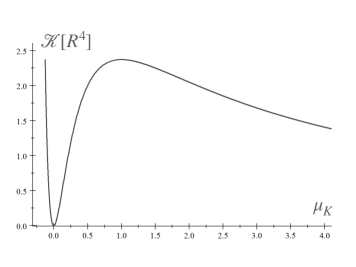
Figure 1: The Kretschmann scalar as function of the Komar mass density (in units of $R^{4}$)

In order to characterize the radial features of the spacetime, we introduce the proper radial distance

$$R=\int_{0}^{r}r^{2\mu_{K}}\mathrm{d}r=\frac{r^{1+2\mu_{K}}}{1+2\mu_{K}}\leavevmode\nobreak\ .$$ (32)

The Kretschmann scalar

$$\mathcal{K}=\frac{64\mu_{K}^{2}}{\left(1+2\mu_{K}\right)^{3}}R^{-4}\leavevmode\nobreak\$$ (33)

scales with $\mu_{K}$, confirming a flat spacetime when it vanishes. It also vanishes in the limit $\mu_{K}\rightarrow\infty$. For all other parameter values the Kretschmann scalar falls off at $R\rightarrow\infty$ and there is a naked singularity on the $Z$ axis.

The dependence of the Kretschmann scalar on the Komar mass density is illustrated for $R=1$ on Fig. 1. It has three extrema: (i) it vanishes at $\mu_{K}=0$, as the spacetime becomes flat; (ii) at $\mu_{K}=-1/8$ there is the maximum in the negative $\mu_{K}$ range; (iii) at $\mu_{K1}=1$ the positive $\mu_{K}$ range has maximal Kretschmann curvature. The existence of $\lambda_{1}=1/4$ (corresponding to $\mu_{K1}$) as the value of the parameter generating maximal Kretschmann curvature has been emphasized by Bonnor and Martins in their discussion of the Levi-Civita metric in the Weyl form Bonnorlambda4 (see Fig. 2 for the Kretschmann scalar as function of $\left(\mu_{K}\right)_{\mathrm{Weyl}}=\lambda$ for $R=1,$ showing a double degeneracy, when compared to Fig. 1). The increase and subsequent decrease of the Kretschmann curvature with $\mu_{K}$ is counterintuitive, undermining the interpretation of $\mu_{K}$ as mass density

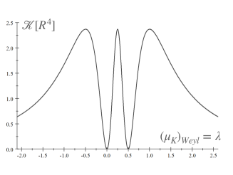
Figure 2: The Kretschmann scalar as function of the Komar mass density defined with the Weyl time (in units of $R^{4}$) shows a double coverage as compared to the Komar mass density defined with the Einstein-Rosen time.

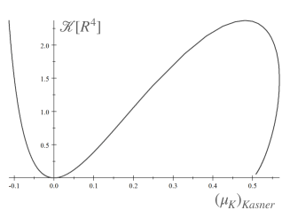
Figure 3: The Kretschmann scalar as function of the Komar mass density defined with the Kasner time (in units of $R^{4}$) is a double valued function for $\left(\mu_{K}\right)_{\mathrm{Kasner}}>0.5$. By contrast $\mathcal{K}$ is well defined everywhere in terms of the Komar mass density $\mu_{K}$ defined with the Einstein-Rosen time

The curvature of a vacuum spacetime, consisting purely of the Weyl tensor $C_{ijkl}$ is characterized by four scalar invariants Harvey :

$$J_{1} = A_{ij}^{\leavevmode\nobreak\ \ ij}\leavevmode\nobreak\ ,\quad J_{2}=B_{ij}^{\leavevmode\nobreak\ \ ij}\leavevmode\nobreak\ ,$$

$$J_{3} = A_{ij}^{\leavevmode\nobreak\ \ kl}A_{kl}^{\leavevmode\nobreak\ \ ij}-\frac{J_{1}^{2}}{2}\leavevmode\nobreak\ ,$$

$$J_{4} = A_{ij}^{\leavevmode\nobreak\ \ kl}B_{kl}^{\leavevmode\nobreak\ \ ij}-\frac{5J_{1}J_{2}}{12}\leavevmode\nobreak\ ,$$ (34)

with

$$A_{ijkl}=C_{ij}^{\leavevmode\nobreak\ \ mn}C_{mnkl}\leavevmode\nobreak\ ,\quad B_{ijkl}=C_{ij}^{\leavevmode\nobreak\ \ mn}A_{mnkl}\leavevmode\nobreak\ .$$ (35)

For the Levi-Civita metric (25) the scalars are

$$J_{1} = \frac{64\mu_{K}^{2}\left(1+2\mu_{K}\right)}{r^{4\left(1+2\mu_{K}\right)}}=\mathcal{K\leavevmode\nobreak\ },$$

$$J_{2} = -\frac{768\mu_{K}^{4}}{r^{6\left(1+2\mu_{K}\right)}}=-\frac{3\mu_{K}}{2}\left(\frac{\mathcal{K}}{1+2\mu_{K}}\right)^{3/2}\leavevmode\nobreak\ ,$$

$$J_{3} = -\frac{1024\mu_{K}^{4}\left(1+2\mu_{K}\right)^{2}}{r^{8\left(1+2\mu_{K}\right)}}=-\frac{\mathcal{K}^{2}}{4}\leavevmode\nobreak\ ,$$

$$J_{4} = 0\leavevmode\nobreak\ .$$ (36)

Hence all invariants are expressed in terms of the Kretschmann scalar and exhibit similar dependence on $\mu_{K}$.

IV.2 Kasner form and Rindler limit of the Levi-Civita spacetime

As in the limit $\mu_{K}\rightarrow\infty$ the metric (25) diverges, we rewrite it in a more suitable form in terms of the proper radial distance (32) and the rescaled time

$$T=\left(1+2\mu_{K}\right)^{\frac{2\mu_{K}}{1+2\mu_{K}}}t\leavevmode\nobreak\ ,$$ (37)

as new coordinates. The line element becomes

$$\mathrm{d}s^{2} = -R^{2p_{0}}\mathrm{d}T^{2}+\mathrm{d}R^{2}+\left[\left(1+2\mu_{K}\right)R\right]^{2p_{+}}\mathrm{d}\psi^{2}$$ (38)

$$+\left[\left(1+2\mu_{K}\right)R\right]^{2p_{-}}\mathrm{d}Z^{2}\leavevmode\nobreak\ ,$$

or

$$\mathrm{d}s^{2}=-R^{2p_{0}}\mathrm{d}T^{2}+\mathrm{d}R^{2}+R^{2p_{+}}\mathrm{d}\chi^{2}+R^{2p_{-}}\mathrm{d}\zeta^{2}\leavevmode\nobreak\ ,$$ (39)

with

$$\chi = \left(1+2\mu_{K}\right)^{p_{+}}\psi\leavevmode\nobreak\ ,$$

$$\zeta = \left(1+2\mu_{K}\right)^{p_{-}}Z\leavevmode\nobreak\ ,$$ (40)

and the coefficients

$$p_{0}=\frac{2\mu_{K}}{1+2\mu_{K}}\leavevmode\nobreak\ ,\quad p_{\pm}=\frac{1\pm\sqrt{1+8\mu_{K}}}{2\left(1+2\mu_{K}\right)}\leavevmode\nobreak\ .$$ (41)

The ranges of the coordinates are $T,\zeta\in\mathbb{R}$, $R\in\mathbb{R}^{+}$ and $\chi\in\left[0,2\pi\left(1+2\mu_{K}\right)^{p_{+}}\right]$. The powers obey $p_{0}+p$${}_{+}+p_{-}=1$ and $p_{0}^{2}+p$${}_{+}^{2}+p_{-}^{2}=1$, implying $p_{0}\in\left[-1/3,1\right]$, $p_{+}\in\left[0,1\right]$, and $p_{-}\in\left[-1/3,2/3\right]$. This form of the Levi-Civita metric resembles the inhomogeneous Kasner metric with coordinates $T$ and $R$ interchanged GriffithsP and is expressed in terms of the Komar mass per unit $Z$ of the Einstein-Rosen coordinates.

For the Levi-Civita metric when $\mu_{K}\rightarrow\infty$, the coefficients reduce to $p_{0}\rightarrow 1$, $p_{\pm}\rightarrow 0$ and $\left(1+2\mu_{K}\right)^{2p_{\pm}}\rightarrow 1$, hence

$$\mathrm{d}s_{\mu_{K}\rightarrow\infty}^{2}=-R^{2}\mathrm{d}T^{2}+\mathrm{d}R^{2}+\mathrm{d}Z^{2}+\mathrm{d}\psi^{2}\leavevmode\nobreak\ .$$ (42)

In this limit it simplifies to a Rindler metric with particular topology $S^{1}\times\mathbb{R}^{3}$, representing flat spacetime perceived by a uniformly accelerated observer with acceleration $R^{-1}$ along $R$. The unusual topology consists of each point of the Rindler wedge $\left(T,R\right)$ corresponding to a cylinder of unit radius (parametrized by longitudinal and angular variables $Z$ and $\psi$, respectively), rather than a plane.

In the $\left(T,R\right)$ coordinates the Komar mass density (associated to the time coordinate vector) emerges as

$$\left(\mu_{K}\right)_{\mathrm{Kasner}}=\frac{p_{0}}{2}\left(1+2\mu_{K}\right)^{p_{-}+p_{+}}=\frac{\mu_{K}}{\left(1+2\mu_{K}\right)^{\frac{2\mu_{K}}{1+2\mu_{K}}}}\leavevmode\nobreak\ .$$ (43)

In the Rindler limit $\mu_{K}\rightarrow\infty$ of an accelerated observer in flat spacetime $\left(\mu_{K}\right)_{\mathrm{Kasner}}=1/2$. This is consistent with the Komar mass surface density $\sigma_{K}$ of the Rindler spacetime given by Eq. (69), multiplied by the circumference $2\pi$ of the additional compactified coordinate.

We have already seen that $\mu_{K}$ bears the advantage over $\left(\mu_{K}\right)_{\mathrm{Weyl}}=\lambda$ of avoiding a double coverage of the parameter space. The parameter $\left(\mu_{K}\right)_{\mathrm{Kasner}}$ suffers from another inconvenience, the Kretschmann scalar $\mathcal{K}$ turning out as a multivalued function of $\left(\mu_{K}\right)_{\mathrm{Kasner}}$ in the range $\left(\mu_{K}\right)_{\mathrm{Kasner}}\geq 1/2$ (which applies to all $\mu_{K}\geq 1.1466$), as can be seen from Fig. 3. Hence we keep $\mu_{K}$ for parametrizing the metric.

With increasing $\mu_{K}$ the Levi-Civita metric approaches the Rindler limit, supporting the statement that beside mass and gravitational energy, the Komar mass density $\mu_{K}$ also encompasses acceleration effects. As the Rindler observers (from the point of view of an inertial observer) accelerate as $R^{-1}$ in the $R$ direction, the Rindler spacetime can also be interpreted through the equivalence principle as a (Newtonian) gravitational field homogeneous in the $T$, $Z$, and $\psi$ directions (hence with the coordinate lines $R$ becoming parallel with $\mu_{K}\rightarrow\infty$). Thus, we conjecture that the magnitude of $\mu_{K}$ correlates with the degree of homogeneity (as defined above) of the Newtonian gravitational field.

IV.3 The singular axis

Recently, Ref. Ahmed has presented the cylindrically symmetric vacuum spacetime

$$\mathrm{d}s^{2}\! = \!\sinh^{2}\!r_{\ast}\!\left(-\mathrm{d}t_{\ast}^{2}\!+\!\mathrm{d}\varphi_{\ast}^{2}\right)+\frac{\mathrm{d}z_{\ast}^{2}}{\sinh r_{\ast}}$$ (44)

$$+\cosh^{2}\!r_{\ast}\sinh r_{\ast}\mathrm{d}r_{\ast}^{2}\leavevmode\nobreak\ ,$$

claiming, among others, that the $r_{\ast}=0$ axis is a geodesically incomplete (for null geodesics) soft singularity both in the sense of Królak Krolak and of Tipler Tipler . However, we show in Appendix C that this metric is but a particular case of the Levi-Civita metric, corresponding to $\mu_{K}=1$, thus referring to the value of the parameter, where the Kretschmann curvature is maximal. We also correct the curvature invariants given in Ref. Ahmed and find that the authors of Ref. Ahmed incorrectly applied the strong singularity criteria.

Therefore we present in this section the rigorous analysis of the singularity on the symmetry axis of the Levi-Civita spacetime, for a generic value of $\mu_{K}$.

Any strong singularity crushes to zero all $3$-volumes (or $2$-volumes, respectively) parallel transported along timelike (or null) geodesics EllisSchmidt . The concept was formulated rigorously by Tipler Tipler . Based on the expectation that in physically realistic spacetimes singularities are both strong and hidden by horizons, Królak proposed a less restrictive condition on the convergence of geodesics Krolak . Clarke and Królak ClarkeKrolak formulated computational recipes corresponding to either the necessary or the sufficient conditions for the Tipler and Królak criteria. For timelike geodesics, there are no conditions that are simulataneously necessary and sufficient, therefore we focus on null geodesics, for which (with special conditions holding on the Weyl tensor), necessary and sufficient conditions may coincide.

In particular, if the Weyl tensor is not identically zero, and it does not display oscillatory behaviour along a null geodesic $\gamma:I\subseteq\mathbb{R}\rightarrow M$ hitting the singularity at affine parameter $\lambda\rightarrow\lambda_{s}$, then the Królak strong singularity condition is satisfied if and only if any component of

$$N_{\ b}^{a}\left(\lambda\right)=\int_{0}^{\lambda}\mathrm{d}\lambda^{\prime}\left(\int_{0}^{\lambda^{\prime}}\mathrm{d}\lambda^{\prime\prime}\left|C_{\ 0b0}^{a}\left(\lambda^{\prime\prime}\right)\right|\right)^{2}$$ (45)

diverge as $\lambda\rightarrow\lambda_{s}$, while the Tipler strong singularity condition holds if and only if any component of

$$L_{\ b}^{a}\left(\lambda\right)=\int_{0}^{\lambda}\mathrm{d}\lambda^{\prime}\int_{0}^{\lambda^{\prime}}\mathrm{d}\lambda^{\prime\prime}\left(\int_{0}^{\lambda^{\prime\prime}}\mathrm{d}\lambda^{\prime\prime\prime}\left|C_{\ 0b0}^{a}\left(\lambda^{\prime\prime\prime}\right)\right|\right)^{2}$$ (46)

diverge as $\lambda\rightarrow\lambda_{s}$. The components $C_{\ bcd}^{a}$ are calculated with respect to a pseudo-orthonormal frame $e_{\mathbf{0}},e_{\mathbf{1}},e_{\mathbf{2}},e_{\mathbf{3}}$ parallel propagated along the geodesic, such that $e_{\mathbf{0}}$ and $e_{\mathbf{1}}$ are the null vectors, $e_{\mathbf{2}}$ and $e_{\mathbf{3}}$ are the spacelike vectors and $e_{\mathbf{0}}=\dot{\gamma}$ is the geodesic’s tangent.

We consider radial null geodesics in the $\left(T,R\right)$-plane of the Kasner-like coordinates:

$$\gamma\left(\lambda\right)=\left(T\left(\lambda\right),R\left(\lambda\right),\chi_{0},\zeta_{0}\right)\leavevmode\nobreak\ ,$$ (47)

where the latter two components are constants. The velocity vector is

$$e_{\mathbf{0}}\left(\lambda\right)=\left(\dot{T}\left(\lambda\right),\dot{R}\left(\lambda\right),0,0\right)\leavevmode\nobreak\ ,$$ (48)

where the overdot denotes derivative with respect to the affine parameter. A radially ingoing null geodesic satisfies the equation

$$\dot{T}=R^{-2p_{0}}\leavevmode\nobreak\ ,\quad\dot{R}=-R^{-p_{0}}\leavevmode\nobreak\ ,$$ (49)

with an irrelevant constant of integration set to unity. Explicitly integrating the geodesic equations is possible, but unnecessary, as the integrals (45) and (46) can be calculated through the chain rule as

$$\int_{0}^{\lambda_{s}}\mathrm{d}\lambda=\int_{0}^{R_{0}}R^{p_{0}\,}\mathrm{d}R\,\leavevmode\nobreak\ ,$$ (50)

where $R_{0}=R\left(0\right)$. A parallel frame along the radial null geodesic is then given by

$$e_{\mathbf{0}} =\left(R^{-2p_{0}},-R^{-p_{0}},0,0\right)\leavevmode\nobreak\ ,$$

$$e_{\mathbf{1}} =\left(\frac{1}{2},\frac{1}{2}R^{p_{0}},0,0\right)\leavevmode\nobreak\ ,$$

$$e_{\mathbf{2}} =\left(0,0,R^{-p_{+}},0\right)\leavevmode\nobreak\ ,$$

$$e_{\mathbf{3}} =\left(0,0,0,R^{-p_{-}}\right)\leavevmode\nobreak\ .$$ (51)

The Weyl tensor, also the integrals (45) and (46) are calculated in the above frame in Appendix D. We found that the components $L_{\ 2}^{2}$ and $L_{\ 3}^{3}$ of the Tipler integrals, as well as the components $N_{\ 2}^{2}$ and $N_{\ 3}^{3}$ of the Królak integrals diverge logarithmically with $R\rightarrow 0$, provided $\mu_{K}\neq 0,\infty$. Hence radial null geodesics satisfy both the Tipler and Królak singularity conditions.

In conclusion, the symmetry axis of the Levi-Civita spacetime represents a strong curvature singularity for any of the allowed parameter values (including $\mu_{K}=1$, which refutes the claim made in Ref. Ahmed about the singularity being soft).

V Physical characterization in terms of the Komar mass density

In this section we analyze the the gravitational effects ocurring in the Levi-Civita spacetime, both from a Newtonian and a general relativistic perspective.

V.1 Gravitational acceleration

In what follows, we investigate the Levi-Civita spacetime by considering a stationary observer at fixed proper distance from the $Z$-axis, with 4-velocity $u^{a}=\left(R^{-p_{0}},0,0,0\right)$ and 4-acceleration

$$a^{a}\equiv u^{b}\nabla_{b}u^{a}=\frac{2\mu_{K}}{1+2\mu_{K}}R^{-1}\delta_{R}^{a}\leavevmode\nobreak\ ,$$ (52)

the latter compensating for the gravitational effect of the cylinder, according to the equivalence principle. The acceleration changing sign with $\mu_{K}$ shows that gravity is repulsive for $-1/8\leq\mu_{K}<0$ and attractive for $\mu_{K}>0$. In the latter case it approximates the Newtonian regime $-d\phi_{N}/dr$ at small $\mu_{K}$ (with $\phi_{N}$ the Newtonian potential generated by a linear mass distribution on the $Z$ axis) and decays at $R\rightarrow\infty$, as expected.

We define the gravitational acceleration (in a Newtonian sense)

$$a_{g}=-\frac{2\mu_{K}}{1+2\mu_{K}}R^{-1}\leavevmode\nobreak\ ,$$ (53)

the magnitude of which represents the magnitude of the acceleration to keep the observer in orbit and its sign being negative (positive) in the attractive (repulsive) regime. This arises from the potential

$$\phi=\frac{2\mu_{K}}{1+2\mu_{K}}\ln R\leavevmode\nobreak\ ,$$ (54)

which reduces to the Newtonian limit $\phi_{N}=2\mu_{K}\ln r$ for small $\mu_{K}$.

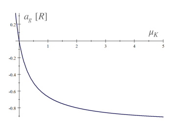
Figure 4: The gravitational acceleration (defined in a Newtonian sense through the equivalence principle) as function of the Komar mass density, in units of $R$.

At unit proper radial distance $a_{g}$ becomes $a_{g}^{R=1}=-2\mu_{K}/\left(1+2\mu_{K}\right)$, illustrated on Fig. 4. The gravitational acceleration at unit proper radial distance is negative (positive) for positive (negative) $\mu_{K}$. For positive $\mu_{K}$ the gravitational acceleration is attractive and increases monotonically with $\mu_{K}$, asymptoting $-1$. Hence, despite increasing $\mu_{K}$, gravitational attraction cannot increase above a certain limit.

V.2 Geodesic deviation

We can better understand the gravitational field by discussing the geodesic deviation. We consider the congruence $U^{a}\equiv\left(\partial/\partial\tau\right)^{a}$, with the proper time $\tau$ given by $d\tau=R^{p_{0}}dT$, implying $U^{a}=R^{-p_{0}}\delta_{T}^{a}$ for any given $R$. Infinitesimally close curves of the congruence are separated by the deviation vector $X^{a}\equiv\left(\partial/\partial R\right)^{a}=\delta_{R}^{a}$. By construction both $U^{a}$ and $X^{a}$ are normalized and they commute. In any arbitrarily chosen point ($\tau=\tau_{1}$, $R=R_{1}$) there is a geodesic with tangent $V^{a}\left(\tau_{1},R_{1}\right)\equiv U^{a}\left(\tau_{1},R_{1}\right)$. In this point the acceleration $D^{2}X^{a}/d\tau^{2}$ can be computed as

$$A^{a} = R_{\leavevmode\nobreak\ bcd}^{a}U^{b}U^{c}X^{d}=R^{-2p_{0}}R_{\leavevmode\nobreak\ TTR}^{a}$$ (55)

$$= p_{0}\left(1-p_{0}\right)R^{-2}\delta_{R}^{a}\leavevmode\nobreak\ ,$$

with magnitude

$$\left(g_{ab}A^{a}A^{b}\right)^{1/2}=\frac{2\left|\mu_{K}\right|}{\left(1+2\mu_{K}\right)^{2}}R^{-2}\leavevmode\nobreak\ .$$ (56)

The negative of this acceleration represents the tidal force acting on a unit mass particle. We visualize its dependence of $\mu_{K}$ at unit proper radial distance on Fig. 5

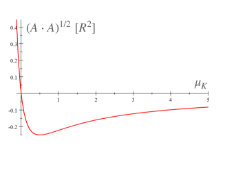
Figure 5: The tidal acceleration among geodesic observers as function of the Komar mass density, in units of $R^{2}$.

The tidal acceleration is zero at $\mu_{K}=0$, as expected for a flat spacetime. Then it increases with $\mu_{K}$ (as for small values it represents the mass density of the cylindric source) up to $\mu_{K2}=1/2$ (corresponding to $\sigma_{2}=\left(1-\sqrt{5}\right)/2$ and $\lambda_{2}=\left(3-\sqrt{5}\right)/4$). Then it decreases again, falling off to zero at $\mu_{K}\rightarrow\infty$. As we discussed before, this renders the Levi-Civita spacetime into Rindler spacetime. In this limit the tidal force vanishes and the gravitational field (in a Newtonian sense) attains a high degree of homogeneity in the $T$, $Z$, and $\psi$ directions.

VI Discussion and concluding remarks

Levi-Civita spacetime can be regarded as the strong field background for a cylindrical gravitational wave, which is the best testbed for comparing quantization methods of gravitational waves. Hence it is paramount to clearly understand this static spacetime. Previous presentations relied on either of the parameters $\lambda$ or $\sigma$, emerging in the Weyl- or Einstein-Rosen coordinates, respectively. Although both parameters, whenever they are small and positive, have the nice interpretation of mass density along the symmetry axis, when considered across their full allowed ranges, are hard to interpret. The reason for this is twofold. First, there is a double coverage of the parameter space, corresponding to a possible interchange of the roles of the axial and polar variables. Then there are two kinds of flat limits, the second one being of Rindler type. This leads to a quartett of parameter values, all leading to flat limit.

Despite the axis being infinite, we could compute the Komar mass density $\mu_{K}$ along the axis through a compactification and a subsequent blowing up of the compactification radius. By introducing $\mu_{K}$ as a new metric parameter, we got rid of the double coverage, but the flat limit still arises in two cases, for $\mu_{K}=0$ and $\mu_{K}\rightarrow\infty$. The first indeed represents no mass on the axis. The second one is a Rindler spacetime, as can be seen manifestly in Kasner type coordinates, which include $R$, the proper radial distance measured from the axis.

The Komar mass density can be in the narrow negative range $-1/8\leq\mu_{K}<0$, when gravity is repulsive. For all positive values it is attractive. In the process of increasing $\mu_{K}$ from $0$ to $\infty$ the Kretschmann scalar increases to $1$, then it decreases again. We identified a recently published solution in Ref. Ahmed as the Levi-Civita spacetime pertinent to the maximal Kretschmann scalar and corrected a number of its claims. In the process we proved that the singularity on the axis is strong for null geodesics both in the Tipler and Królak senses, for any $\mu_{K}$.

In order to understand the Rindler limit at $\mu_{K}\rightarrow\infty$, however $R$ cannot be regarded as radial any more. Initially $\left(R,\psi\right)$ cover $\mathbb{R}^{2}$ as polar coordinates, while in the Rindler limit they cover a cylinder $S^{1}\times\mathbb{R}$. This process can be visualized (through an embedding into higher dimensions) as a pinching of the $\left(R,\psi\right)$ plane into a direction perpendicular to both the plane and the $Z$ axis, creating a cone-like shape. As $\mu_{K}$ further increases, the tip of the cone opens up into a funnel, which attains its climax as a constant cross-section tube, in which the $R$ coordinate lines become parallel. In the Rindler limit inertial observers have coordinate acceleration $R^{-1}$ in the negative $R$ direction, appearing as gravity (in the Newtonian sense), with the tidal acceleration vanishing.

To illustrate the effect of increasing $\mu_{K}$, we calculate the circumference of the circles with coordinate radius $R$ from Eq. (38) as

$$C\left(R;\mu_{K}\right)=2\pi\left[\left(1+2\mu_{K}\right)R\right]^{\frac{1+\sqrt{1+8\mu_{K}}}{2\left(1+2\mu_{K}\right)}}\leavevmode\nobreak\ .$$ (57)

Then we plot the circumference as function of both $R$ and $\mu_{K}$ on Fig. 6. While for $\mu_{K}=0$ the circumference takes the flat value $C\left(R;0\right)=2\pi R$, at $\mu_{K}\rightarrow\infty$ it becomes $\lim_{\mu_{K}\rightarrow\infty}C\left(R;\mu_{K}\right)=2\pi\lim_{\mu_{K}\rightarrow\infty}\mu_{K}^{1/\sqrt{2\mu_{K}}}=2\pi$. We also represent the process of how the Euclidean radius of the circles (defined as $C\left(R;\mu_{K}\right)/2\pi$) changes with the coordinate $R$ for increasing values of $\mu_{K}$ on both an animation (with increasing $\mu_{K}$ as time variable), given as supplementary material, and on a sequence of figures (Fig. 7.)

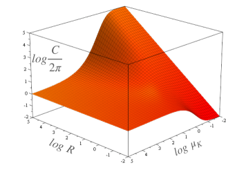
Figure 6: The transformation of the geometry induced by an increasing Komar mass density $\mu_{K}$. The circumference $C$ of a circle is approximately $2\pi$ times the radius $R$ for small $\mu_{K}$, as shown on the right side of the plotted surface, representing an almost flat, cylindrically symmetric spacetime. With increasing $\mu_{K}$ the increase of the cicumference with radius becomes slower, eventually the circumference becoming a constant, regardless of the value of the coordinate $R$. The latter limit corresponds to the Rindler spacetime with poinwise acceleration $R^{-1}$ in the $R$ direction.

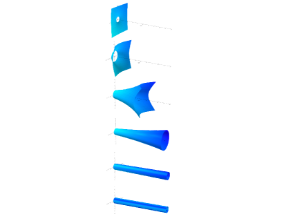
Figure 7: The coordinates $Z$ and $T$ are supressed, while $R$ and $\psi$ are embedded in a three-dimensional Euclidean space. The sequence of figures (from top to bottom) represents the evolution with increasing $\mu_{K}$ of the dependence of the Euclidean radius (defined as $C\left(R;\mu_{K}\right)/2\pi$, the circumference of the circles over $2\pi$, represented in the vertical plane) on the coordinate radius $R$ (represented on logarithmic scale on the horizontal axis). At small $\mu_{K}$ (top figure) the metric is almost flat. With increasing $\mu_{K}$ (lower figures) gravity bends spacetime into a funnel (with the tip at $R=0$), which eventually degenerates into a cylinder, with unit radius for $\mu_{K}\rightarrow\infty$ (bottom figure). While for any $\mu_{K}\neq 0$ the tip $R=0$ of the funnel represents a singularity, the larger hole appearing at the base of the funnel at small $R$ is but a numerical artefact arising from the lower theshold in the chosen range of $R$ to be represented.

We summarize the findings of the paper by presenting the various regimes of the Levi-Civita spacetime on Fig. 8. On the horizontal axis the Kasner parameter $p_{0}$ increases from $-1/3$ to $1$. The red and blue curves represent $p_{+}$ and $p_{-}$, respectively. The Komar mass density also increases from left to right, monotonically with $p_{0}$. From left to right the figure shows the following regimes:

• the limit of maximal repulsion, for $\mu_{K}=-1/8$, thus $p_{0}=-1/3$

• the repulsive gravity regime, for $\mu_{K}\in[-1/8,0)$, thus $p_{0}\in[-1/3,0)$

• the flat limit, for $\mu_{K}=0$, thus $p_{0}=0$

• the regime, where gravitational attraction dominates, for $\mu_{K}\in(0,1)$, thus $p_{0}\in(0,2/3)$

• the maximal value of the Kretschmann scalar (the metric of Ref. Ahmed ), for $\mu_{K}=1$, thus $p_{0}=2/3$

• the regime, where Newtonian gravity drags the field lines increasingly parallel, for $\mu_{K}\in(1,\infty)$, thus $p_{0}\in(2/3,1)$

• the Rindler limit, where the perfectly parallel field lines transform gravity into a pure acceleration field through the equivalence principle, for $\mu_{K}\rightarrow\infty$, thus $p_{0}=1$.

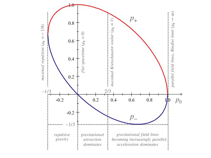
Figure 8: The various regimes of the Levi-Civita metric in terms of the Kasner parameters $p_{+}$ (red curve), $p_{-}$ (blue curve) and $p_{0}$ (horizontal axis). The Komar mass density increases from left to right, spanning to the regime of negative gravity $\mu_{K}\in[-1/8,0)$, no gravity $\mu_{K}=0$, gravitational attraction dominated regime $\mu_{K}\in(0,1)\,$, maximal Kretschmann scalar (the metric of Ref. Ahmed ) $\mu_{K}=1$, increasingly parallel field lines transforming gravity into an acceleration field $\mu_{K}\in(1,\infty)$, and perfectly parallel field lines, the Rindler limit $\mu_{K}\rightarrow\infty$.

Hence, from the combined analysis of the gravitational acceleration (53), which increases monotonically with $\mu_{K}$ but asymptotes to a constant; and of the tidal force (which falls off completely in the asymptotic regime $\mu_{K}\rightarrow\infty$), as shown by the geodesic deviation acceleration (56) we conclude, that adding to the Komar mass density strengthens the gravitational acceleration, as expected, however drives the field lines increasingly parallel. The first effect dominates at small $\mu_{K}$, while the second at large $\mu_{K}$. The Riemannian curvature decays with increasing $\mu_{K}$, the gravitational field becoming fully equivalent to a Rindler frame of accelerating observers in flat spacetime. Hence, in a Newtonian sense the field lines become parallel, while in an Einsteinian sense gravity vanishes.

VII Acknowledgements

This work was supported by the Hungarian National Research Development and Innovation Office (NKFIH) in the form of Grant No. 123996 and has been carried out in the framework of COST action CA18108 (QG-MM) supported by COST (European Cooperation in Science and Technology). Computations of curvature components were performed with the computer algebra system Cadabra2 Cad1 ; Cad2 .

Appendix A Derivation of the Einstein–Rosen form of the cylindrically symmetric metric

Thorne Thorne has given the line element for a generic cylindrically symmetric spacetime with vorticity-free Killing vectors and orthogonally transitive group action (dubbed as whole-cylinder symmetry) in a standard form

$$\mathrm{d}s^{2}=e^{2\left(\tilde{K}-U\right)}\left(-\mathrm{d}\tilde{t}^{2}+\mathrm{d}\tilde{r}^{2}\right)+e^{-2U}W^{2}\mathrm{d}\varphi^{2}+e^{2U}\mathrm{d}z^{2}\leavevmode\nobreak\ ,$$ (58)

with $U$, $\tilde{K}$ and $W$ functions of $\left(\tilde{t},\tilde{r}\right)$ only. For certain particular sources this can be reduced to the simpler Einstein–Rosen (canonical) form (1). For the completeness of presentation we discuss in this Appendix explicitly the reduction and coordinate transformation leading to the canonical form of the cylindrically symmetric line element.

As Thorne has emphasized, when the energy density equals the radial pressure, thus $T_{\tilde{t}}^{\tilde{t}}+T_{\tilde{r}}^{\tilde{r}}=0\,$ (a condition holding both for vacuum and electromagnetic field), the Einstein equation $R_{\tilde{t}}^{\tilde{t}}+R_{\tilde{r}}^{\tilde{r}}-R=0$ implies that the function $W$ with differential

$$\mathrm{d}W=\frac{\partial W}{\partial\tilde{t}}\mathrm{d}\tilde{t}+\frac{\partial W}{\partial\tilde{r}}\mathrm{d}\tilde{r}$$ (59)

obeys the wave equation $W_{,\tilde{t}\tilde{t}}=W_{,\tilde{r}\tilde{r}}$. Hence $W$ is a harmonic function, advantageous to use as a new coordinate.

We introduce another new coordinate $t$ through

$$\frac{\partial t}{\partial\tilde{t}}=\frac{\partial W}{\partial\tilde{r}}\leavevmode\nobreak\ ,\quad\frac{\partial t}{\partial\tilde{r}}=\frac{\partial W}{\partial\tilde{t}}\leavevmode\nobreak\ .$$ (60)

The new coordinate is well-defined, since the harmonicity of $W$ is but the integrability condition for $t$. Moreover, $t$ is also harmonic through Eq. (60). From Eqs. (59) and (60) it is immediate to show that

$$-\mathrm{d}t^{2}+\mathrm{d}r^{2}=e^{2\alpha}\left(-\mathrm{d}\tilde{t}^{2}+\mathrm{d}\tilde{r}^{2}\right)\leavevmode\nobreak\ ,$$ (61)

with $\alpha$ a function of $\left(\tilde{t},\tilde{r}\right)$ given as

$$e^{2\alpha}=-\left(\frac{\partial W}{\partial\tilde{t}}\right)^{2}+\left(\frac{\partial W}{\partial\tilde{r}}\right)^{2}\leavevmode\nobreak\ .$$ (62)

Hence the set of harmonic coordinates $\left(t,r\equiv W\right)$, similarly to the old coordinates $\left(\tilde{t},\tilde{r}\right)$, are conformally flat.

In defining $\alpha$ we assumed the right hand side of Eq. (62) positive, implying the 4-gradient of $W$ to be spacelike. It follows that $t$ is a temporal coordinate.

Eq. (62) is trivially satisfied by parametrizing the 4-gradient of $W$ through

$$\frac{\partial W}{\partial\tilde{r}} = e^{\alpha}\cosh\beta\leavevmode\nobreak\ ,$$

$$\frac{\partial W}{\partial\tilde{t}} = e^{\alpha}\sinh\beta\leavevmode\nobreak\ ,$$ (63)

with $\beta$ a function of $\left(\tilde{t},\tilde{r}\right)$. The coordinate transformation then emerges as a sequence of a hyperbolic rotation and a dilation on the coordinate differentials:

$$\left(\begin{array}[]{c}dt\\ dr\end{array}\right)=e^{\alpha}\left(\begin{array}[]{cc}\cosh\beta&\sinh\beta\\ \sinh\beta&\cosh\beta\end{array}\right)\left(\begin{array}[]{c}d\tilde{t}\\ d\tilde{r}\end{array}\right)\leavevmode\nobreak\ .$$ (64)

With $K=\tilde{K}-\alpha$ and $U$ functions of $\left(t,r\right)$ the line element in the new coordinates takes the canonical (Einstein-Rosen) form (1).

Appendix B Komar mass density of the Rindler metric

In this appendix we calculate a suitably defined Komar mass surface density in flat spacetime, expressed in a reference frame uniformly accelerated into the $x$ direction with acceleration $x^{-1}$, hence in Rindler coordinates:

$$\mathrm{d}s^{2}=-x^{2}\mathrm{d}t^{2}+\mathrm{d}x^{2}+\mathrm{d}y^{2}+\mathrm{d}z^{2}\leavevmode\nobreak\ ,$$ (65)

where $t$ is now the Rindler time. This metric covers the right quadrant of the Minkowski spacetime, corresponding to $x>0$ in the Rindler coordinates and has a coordinate singularity at the hyperplane $x=0$, which represents an infinitely accelerated observer.

We define $y=l\varphi$ and $z=k\psi$, with $l$ and $k$ length scales, $0\leq\varphi\leq 2\pi$ and $0\leq\psi\leq 2\pi$ angular coordinates with period $2\pi$. This compactifies the spacetime in both the $y$ and $z$ direction with the original spacetime recovered for $l,k\rightarrow\infty$. In terms of the compactified coordinates the line element becomes

$$\mathrm{d}s^{2}=-x^{2}\mathrm{d}t^{2}+\mathrm{d}x^{2}+l^{2}\mathrm{d}\varphi^{2}+k^{2}\mathrm{d}\psi^{2}\leavevmode\nobreak\ .$$ (66)

The timelike Killing vector $\xi=\partial_{t}$ has the length squared $\xi\cdot\xi=-x^{2}$ forbidding a distinguished normalization for $\xi$. The Komar superpotential reads

$$\mathbf{U}_{\xi}=\ast\mathrm{d}\bm{\xi}=-2kl\mathrm{d}\varphi\wedge\mathrm{d}\psi\leavevmode\nobreak\ ,$$ (67)

which integrated on $t=\mathrm{const}$, $x=\mathrm{const}$, $0\leq\varphi\leq 2\pi$, and $0\leq\psi\leq 2\pi$ gives

$$m_{K}=\pi kl\leavevmode\nobreak\ .$$ (68)

The coordinate area of the torus $0\leq\varphi,\psi\leq 2\pi$ in the original coordinates $y,z$ is $4\pi^{2}kl$, we thus define the surface Komar mass density as

$$\left(\sigma_{K}\right)_{{}_{\mathrm{Rindler}}}=\frac{m_{K}}{4\pi^{2}kl}=\frac{1}{4\pi}.$$ (69)

We may now take $k,l\rightarrow\infty$ to recover the original Rindler spacetime, a procedure which does not affect $\left(\sigma_{K}\right)_{{}_{\mathrm{Rindler}}}$.

With respect to the timelike coordinate vector of the standard pseudo-Cartesian coordinates, Minkowski spacetime has zero Komar mass. Indeed, the timelike Killing vector is naturally normalized everywhere.

When no obvious normalization of the Killing vector (ensured for example by a proper asymptotic behaviour) is available, Komar integrals can lead to finite, conserved charges that capture some aspects of the reference frame (in this case, acceleration), but such charges do not necessarily characterize invariant geometric aspects of the gravitational field.

Appendix C A particular case: the maximal Kretschmann parameter

In this appendix we show that the cylindrically symmetric vacuum spacetime discussed in Ref. Ahmed is but a particular case of the Levi-Civita metric. We also refute some of their claims about the spacetime.

We start by introducing new coordinates as

$$T = \left(\frac{3}{2}\right)^{2/3}t_{\ast}\leavevmode\nobreak\ ,\quad R=\frac{2}{3}\sinh^{3/2}r_{\ast}\leavevmode\nobreak\ ,$$

$$\chi = \left(\frac{3}{2}\right)^{2/3}\varphi_{\ast}\leavevmode\nobreak\ ,\quad\zeta=\left(\frac{3}{2}\right)^{-1/3}z_{\ast}\leavevmode\nobreak\ ,$$ (70)

(with $\chi\in\left[0,2\pi\left(3/2\right)^{2/3}\right]$), rendering the line element (44) into (39), with the particular coefficients $p_{0}=p_{+}=2/3$ and $p_{-}=-1/3$, leading to $\mu_{K}=1$. Hence the metrics (25) and (44) are locally equivalent for this particular parameter value, nevertheless there is a disagreement in the angular deficits in $\chi$ in their Kasner form.

At $\mu_{K}=1$, the particular case of the Levi-Civita metric discussed in Ref. Ahmed , the Kretschmann scalar exhibits its maximum:

$$\mathcal{K}=\left(\frac{4}{3}\right)^{3}R^{-4}=\frac{12}{\sinh^{6}r_{\ast}}\leavevmode\nobreak\$$ (71)

and the curvature invariants (36) are

$$J_{1} = \mathcal{K\leavevmode\nobreak\ },\quad J_{2}=-\frac{\mathcal{K}^{3/2}}{2\sqrt{3}}=-\frac{12}{\sinh^{9}r_{\ast}}\leavevmode\nobreak\ ,$$ (72)

$$J_{3} = -\frac{\mathcal{K}^{2}}{4}=-\frac{36}{\sinh^{12}r_{\ast}}\leavevmode\nobreak\ ,\quad J_{4}=0\leavevmode\nobreak\ .$$ (73)

With this, we correct the values of $J_{2}$ and $J_{4}$ given in Ref. Ahmed .

The C-energy (26) in the particular case $\mu_{K}=1$ reads

$$E_{C}^{\mu_{K}=1}=\ln r\leavevmode\nobreak\ =\frac{\ln 2}{3}+\frac{1}{2}\ln\sinh r_{\ast},$$ (74)

also different from the one given in Ref. Ahmed , which however seems to be calculated from $E_{C}^{\mathrm{alt}}$.

Ref. Ahmed additionally claimed that the singularity on the axis is soft. We also refute this statement in section IV.3 and Appendix D.

Appendix D Strong singularity conditions

In this Appendix we give the details of the calculations of the Tipler and Królak integrals necessary to classify the singularity on the axis.

In the special case when the Weyl tensor is not identically zero, does not show oscillatory behaviour along the geodesic and the geodesic is null, a unified necessary and sufficient condition for a strong singularity both in the sense of Tipler (46) and of Królak (45) can be given, in terms of the components $C_{\ bcd}^{a}$ of the Weyl tensor in a parallel propagated pseudoorthonormal frame $\left\{e_{\mathbf{a}}\right\}$, with dual $\left\{\theta^{\mathbf{a}}\right\}$. Such a frame, with $e_{\mathbf{0}}$ the tangent of the (affinely parametrized) null geodesic (written in terms of Kasner-like coordinates) was presented as Eq. (51) and can be conveniently extended to a neighborhood of the geodesic.

The curvature forms $\Omega_{\ \mathbf{b}}^{\mathbf{a}}=\mathrm{d}\omega_{\leavevmode\nobreak\ \mathbf{b}}^{\mathbf{a}}+\omega_{\leavevmode\nobreak\ \mathbf{c}}^{\mathbf{a}}\wedge\omega_{\leavevmode\nobreak\ \mathbf{b}}^{\mathbf{c}}$ (with $\omega_{\leavevmode\nobreak\ \mathbf{b}}^{\mathbf{a}}$ the connection 1-forms) are

$$\Omega_{\ \mathbf{0}}^{\mathbf{0}} =\frac{p_{0}\left(p_{0}-1\right)}{R^{2}}\theta^{\mathbf{0}}\wedge\theta^{\mathbf{1}}\leavevmode\nobreak\ ,$$

$$\Omega_{\ \mathbf{2}}^{\mathbf{0}} =\frac{p_{+}p_{-}}{2R^{2}}\theta^{\mathbf{0}}\wedge\theta^{\mathbf{2}}-\frac{\left(2p_{0}+p_{-}\right)p_{+}}{4R^{2\left(1-p_{0}\right)}}\theta^{\mathbf{1}}\wedge\theta^{\mathbf{2}}\leavevmode\nobreak\ ,$$

$$\Omega_{\ \mathbf{3}}^{\mathbf{0}} =\frac{p_{+}p_{-}}{2R^{2}}\theta^{\mathbf{0}}\wedge\theta^{\mathbf{3}}-\frac{\left(2p_{0}+p_{+}\right)p_{-}}{4R^{2\left(1-p_{0}\right)}}\theta^{\mathbf{1}}\wedge\theta^{\mathbf{3}}\leavevmode\nobreak\ ,$$

$$\Omega_{\ \mathbf{2}}^{\mathbf{1}} =\frac{p_{+}p_{-}}{2R^{2}}\theta^{\mathbf{1}}\wedge\theta^{\mathbf{2}}-\frac{\left(2p_{0}+p_{-}\right)p_{+}}{R^{2\left(1+p_{0}\right)}}\theta^{\mathbf{0}}\wedge\theta^{\mathbf{2}}\leavevmode\nobreak\ ,$$

$$\Omega_{\ \mathbf{3}}^{\mathbf{1}} =\frac{p_{+}p_{-}}{2R^{2}}\theta^{\mathbf{1}}\wedge\theta^{\mathbf{3}}-\frac{\left(2p_{0}+p_{+}\right)p_{-}}{R^{2\left(1+p_{0}\right)}}\theta^{\mathbf{0}}\wedge\theta^{\mathbf{3}}\leavevmode\nobreak\ ,$$

$$\Omega_{\ \mathbf{3}}^{\mathbf{2}} =-\frac{p_{+}p_{-}}{R^{2}}\theta^{\mathbf{2}}\wedge\theta^{\mathbf{3}}\leavevmode\nobreak\ ,$$ (75)

with the frame indices raised and lowered by the flat metric

$$\left(k_{ab}\right)=\left(k^{ab}\right)=\begin{pmatrix}0&-1&0&0\\ -1&0&0&0\\ 0&0&1&0\\ 0&0&0&1\end{pmatrix}\leavevmode\nobreak\ ,$$ (76)

which for an arbitrary vector $V^{a}$ results in the rules

$$V_{0}=-V^{1}\leavevmode\nobreak\ ,\quad V_{1}=-V^{0}\leavevmode\nobreak\ ,\quad V_{2}=V^{2}\leavevmode\nobreak\ ,\quad V_{3}=V^{3}\leavevmode\nobreak\ .$$ (77)

The Levi-Civita spacetime being Ricci-flat, the curvature forms $\Omega_{\ \mathbf{b}}^{\mathbf{a}}=\frac{1}{2}R_{\ bcd}^{a}\theta^{\mathbf{c}}\wedge\theta^{\mathbf{d}}$ represent Weyl tensor components, nonvanishing along the geodesic (except for special parameter values for which the spacetime is flat, but then there is no singularity either), also they do not oscillate. Hence the criteria for the diverging of the Tipler and Królak integrals representing unified necessary and sufficient conditions for a strong singularity are met.

Except the flat case, thus either of the cases $\left(p_{0},p_{+},p_{-}\right)=\left(0,1,0\right)$ or $\left(1,0,0\right)$, all components of the Weyl tensor blow up with $R\rightarrow 0$. In what follows, we discuss, whether this singularity is strong or soft.

The explicit calculation gives the nonvanishing Królak integrals

$$N_{\ 1}^{0}=D-CR^{2p_{0}}-\frac{C^{2}}{p_{0}+1}R^{p_{0}+1}-p_{0}^{2}F_{1}\left(R;p_{0}\right)\leavevmode\nobreak\ ,$$ (78)

where $C$ and $D$ are constants of integration, and

$$F_{1}\left(R;p_{0}\right)=\begin{cases}\frac{R^{3p_{0}-1}}{3p_{0}-1}\leavevmode\nobreak\ ,&p_{0}\neq 1/3\\ \ln R\leavevmode\nobreak\ ,&p_{0}=1/3\end{cases}\leavevmode\nobreak\ ,$$ (79)

together with

$$N_{\ 2}^{2} =D+\frac{p_{+}^{2}\left(2p_{0}+p_{-}\right)^{2}}{\left(p_{0}+1\right)^{3}}R^{-\left(p_{0}+1\right)}-\frac{C^{2}}{p_{0}+1}R^{p_{0}+1}$$

$$-2C\frac{p_{+}\left(2p_{0}+p_{-}\right)}{p_{0}+1}\ln R\leavevmode\nobreak\ ,$$

$$N_{\ 3}^{3} =D+\frac{p_{-}^{2}\left(2p_{0}+p_{+}\right)^{2}}{\left(p_{0}+1\right)^{3}}R^{-\left(p_{0}+1\right)}-\frac{C^{2}}{p_{0}+1}R^{p_{0}+1}$$

$$-2C\frac{p_{-}\left(2p_{0}+p_{+}\right)}{p_{0}+1}\ln R\leavevmode\nobreak\ .$$ (80)

At $R\rightarrow 0$, the integrals $N_{\ 2}^{2}$ and $N_{\ 3}^{3}$ contain both power-law and logarithmic divergences, while $N_{\ 1}^{0}$ can blow up for any $p_{0}\leq 1/3$ parameter values.

Likewise, the Tipler integrals $L_{\ b}^{a}$ are

$$L_{\ 1}^{0} = E-\frac{D}{p_{0}+1}R^{p_{0}+1}+\frac{C}{3p_{0}+1}R^{3p_{0}+1}$$ (81)

$$+\frac{C^{2}R^{2p_{0}+2}}{2\left(p_{0}+1\right)^{2}}+\frac{p_{0}}{4}R^{4/3}F_{2}\left(R;p_{0}\right)\leavevmode\nobreak\ ,$$

where $C,D$ and $E$ are constants of integration, and

$$F_{2}\left(R;p_{0}\right)=\begin{cases}\frac{R^{4\left(3p_{0}-1\right)/3}}{3p_{0}-1}\leavevmode\nobreak\ ,&p_{0}\neq 1/3\\ \ln R\leavevmode\nobreak\ ,&p_{0}=1/3\end{cases}\leavevmode\nobreak\ ,$$ (82)

together with

$$L_{\ 2}^{2} = \int_{R}^{R_{0}}\mathrm{d}R\,\left[DR^{p_{0}}+\frac{\left(2p_{0}+p_{-}\right)^{2}p_{+}^{2}}{\left(p_{0}+1\right)^{3}R}-\frac{C^{2}R^{2p_{0}+1}}{p_{0}+1}\right.$$ (83)

$$\left.-2C\frac{\left(2p_{0}+p_{-}\right)p_{+}}{p_{0}+1}R^{p_{0}}\ln R\right]\leavevmode\nobreak\ ,$$

(with $R_{0}$ characterizing the initial point of the geodesic) and $L_{\ 3}^{3}$ obtained from $L_{\ 2}^{2}$ through the exchange $p_{+}\leftrightarrow p_{-}$. We can see even without calculating the integrals a logarithmic divergence emerging in both $L_{\ 2}^{2}$ and $L_{\ 3}^{3}$ at $R\rightarrow 0$, while $L_{\ 1}^{0}$ blows up only for $p_{0}\leq 1/3$. We conclude that for radial null geodesics the strong singularity conditions are satisfied both in the sense of Królak and of Tipler.

References

- (1) A. Einstein, Näherungsweise Integration der Feldgleichungen der Gravitation, Sitzung der physikalisch-mathematischen Klasse, 668-96 (CPAE 6 Doc. 32, 348-57) (1916).
- (2) LIGO Scientific Collaboration, Virgo Collaboration, KAGRA Collaboration, GWTC-3: Compact Binary Coalescences Observed by LIGO and Virgo During the Second Part of the Third Observing Run, [arXiv:2111.03606 [gr-qc]].
- (3) A. Einstein and N. Rosen, On gravitational waves, J. Franklin Inst. 223, 43 (1937).
- (4) V. A. Belinskii and E. E. Zakharov, Integration of the Einstein equations by means of the inverse scattering problem technique and construction of exact soliton solutions, Sov. Phys. JETP. 48, 985 (1978).
- (5) M. Carmeli, Classical Fields: General Relativity and Gauge Theory (John Wiley & Sons, New York, 1982).
- (6) L. Herrera and N. O. Santos, Cylindrical Collapse and Gravitational Waves, Class. Quantum Grav. 22, 2407 (2005), [arXiv:gr-qc/0502009].
- (7) K. Kuchař, Canonical Quantization of Cylindrical Gravitational Waves, Phys. Rev. D 4, 955 (1971). The notations ot this paper are related to ours as , , and .
- (8) B. S. DeWitt, Quantum Theory of Gravity. I. The Canonical Theory, Phys. Rev. 160, 1113 (1967).
- (9) C. W. Misner, Mixmaster Universe, Phys. Rev. Lett. 22, 1071 (1969).
- (10) C. W. Misner, Quantum Cosmology. I, Phys. Rev. 186, 1319 (1969).
- (11) C. W. Misner, Absolute Zero of Time, Phys. Rev. 186, 1328 (1969).
- (12) R. A. Isaacson, Gravitational Radiation in the Limit of High Frequency. I. The Linear Approximation and Geometrical Optics, Phys. Rev. 166, 1263 (1968).
- (13) R. A. Isaacson, Gravitational Radiation in the Limit of High Frequency. II. Nonlinear Terms and the Effective Stress Tensor, Phys. Rev. 166, 1272 (1968).
- (14) T. Levi-Civita, Atti Accad. Naz. Lincei, Cl. Sci. Fis. Mat. Nat. Rend. 28, 101 (1919). English-translation: Gen. Rel. Grav. 43, 2321(2011).
- (15) J. Krishna Rao, Radiating Levi-Civita metric, J. Phys. A: Gen. Phys. 4, 17 (1971). The notations ot this paper are related to ours as , , and
- (16) W. B. Bonnor, Certain Exact Solutions of the Equations of General Relativity with an Electrostatic Field, Proc. Phys. Soc. A 66, 145 (1953).
- (17) A. K. Raychaudhuri, Static electromagnetic fields in general relativity, Ann. Phys. 11, 501 (1960).
- (18) L. Marder, Gravitational waves in general relativity. I. Cylindrical waves, Proc. R. Soc. Lond. A 244, 524 (1958).
- (19) K. S. Thorne, Energy of Infinitely Long, Cylindrically Symmetric Systems in General Relativity, Phys. Rev. 138, B251 (1965). The notations ot this paper are related to ours as and (when ).
- (20) W. B. Bonnor, Solution of Einstein’s equations for a line-mass of perfect fluid, J. Phys. A: Math. Get. 12 847 (1979).
- (21) J. B. Griffiths and J. Podolský, Exact Space-Times in Einsein’s General Relativity, Cambridge University Press (2009).
- (22) R. Gautreau and R. B. Hoffman, Exact solutions of the Einstein vacuum field equations in Weyl co-ordinates, Nuovo Cimento B61, 411 (1969).
- (23) W. B. Bonnor and M. A. P. Martins, The interpretation of some static vacuum metrics, Class. Quantum Grav. 8, 727 (1991).
- (24) D. Bini, A. Geralico and W. Plastino, Cylindrical gravitational waves: C-energy, super-energy and associated dynamical effects, Class. Quantum Grav. 36, 095012 (2019), [arXiv:1812.07938 [gr-qc]].
- (25) F. Ahmed and F. Rahaman, Gravitational collapse in a cylindrical symmetric vacuum space-time and the naked singularity, Eur. Phys. J. A 54, 52 (2018).
- (26) A. Królak, A Proof of the Cosmic Censorship Hypothesis, Gen. Rel. Grav. 15, 99 (1983).
- (27) F. Tipler, Singularities in Conformally Flat Space-times, Phys. Lett. 64A, 8 (1977).
- (28) L. Akyar and Ö. Delice, On generalized Einstein–Rosen waves in Brans–Dicke theory, Eur. Phys. J. Plus 129, 226 (2014).
- (29) H. Stephani, D. Kramer, M. MacCallum, C. Hoenselaers, E. Hertl, Exact Solutions to Einstein’s Field Equations, 2nd ed., Cambridge University Press (2003).
- (30) A. Komar, Covariant Conservation Laws in General Relativity, Phys. Rev. 113, 934 (1959).
- (31) L. Fatibene and M. Francaviglia, Natural and Gauge Natural Formalism for Classical Field Theories, Springer (2003).
- (32) L. F. O. Costa, J. Natário, N. O. Santos, Gravitomagnetism in the Lewis cylindrical metrics, Class. Quantum Grav. 38, 055003 (2021).
- (33) S. Chandrasekhar, Cylindrical Waves in General Relativity, Proc. R. Soc. Lond. A 408, 209 (1986).
- (34) S. A. Hayward, Gravitational waves, black holes and cosmic strings in cylindrical symmetry, Class. Quantum Grav. 17, 1749 (2000).
- (35) T. Chiba, Cylindrical Dust Collapse in General Relativity: Toward Higher Dimensional Collapse, Prog. Theor. Phys. 95, 321 (1996).
- (36) A. Harvey, On the algebraic invariants of the four-dimensional Riemann tensor, Class. Quantum Grav. 7, 715 (1990).
- (37) G. F. R. Ellis and B. G. Schmidt, Singular Space-times, Gen. Rel. Grav. 8, 915 (1977).
- (38) C. J. S. Clarke and A. Królak, Conditions for the occurence of strong curvature singularities, J. Geom. Phys. 2, 127 (1985).
- (39) K. Peeters, Introducing Cadabra: a symbolic computer algebra system for field theory problems, arXiv:hep-th/0701238 (2007)
- (40) K. Peeters, Cadabra: a field-theory motivated symbolic computer algebra system, Comp. Phys. Commun. 176, 550-558 (2007)