Decompiling x86 Deep Neural Network Executables

Abstract

Due to their widespread use on heterogeneous hardware devices, deep learning (DL) models are compiled into executables by DL compilers to fully leverage low-level hardware primitives. This approach allows DL computations to be undertaken at low cost across a variety of computing platforms, including CPUs, GPUs, and various hardware accelerators.

We present BTD (Bin to DNN), a decompiler for deep neural network (DNN) executables. BTD takes DNN executables and outputs full model specifications, including types of DNN operators, network topology, dimensions, and parameters that are (nearly) identical to those of the input models. BTD delivers a practical framework to process DNN executables compiled by different DL compilers and with full optimizations enabled on x86 platforms. It employs learning-based techniques to infer DNN operators, dynamic analysis to reveal network architectures, and symbolic execution to facilitate inferring dimensions and parameters of DNN operators.

Our evaluation reveals that BTD enables accurate recovery of full specifications of complex DNNs with millions of parameters (e.g., ResNet). The recovered DNN specifications can be re-compiled into a new DNN executable exhibiting identical behavior to the input executable. We show that BTD can boost two representative attacks, adversarial example generation and knowledge stealing, against DNN executables. We also demonstrate cross-architecture legacy code reuse using BTD, and envision BTD being used for other critical downstream tasks like DNN security hardening and patching.

1 Introduction

Recent years have witnessed increasing demand for applications of deep learning (DL) in real-world scenarios. This demand has led to extensive deployment of DL models in a wide spectrum of computing platforms, ranging from cloud servers to embedded devices. Deployment of models in such a spread of platforms is challenging, given the diversity of hardware characteristics involved (e.g., storage management and compute primitives) including GPUs, CPUs, and FPGAs.

A promising trend is to use DL compilers to manage and optimize these complex deployments on multiple platforms [22, 85, 64]. A DL compiler takes a high-level model specification (e.g., in ONNX format [6]) and generates corresponding low-level optimized binary code for a variety of hardware backends. For instance, TVM [22], a popular DL compiler, generates DNN executable with performance comparable to manually optimized libraries; it can compile models for heterogeneous hardware backends. To date, DL compilers are already used by many edge devices and low-power chips vendors [75, 48, 83, 74]. Cloud service providers like Amazon and Google are also starting to use DL compiler in their AI services for performance improvements [14, 101]. In particular, Amazon and Facebook are seen to spend considerable effort to compile DL models on Intel x86 CPUs through the usage of DL compilers [61, 49, 69].

Compilation of high-level models into binary code typically involves multiple optimization cycles [22, 85, 64]. DL compilers can optimize code utilizing domain-specific hardware features and abstractions. Hence, generated executables manifest distinct representations of the high-level models from which they were derived. However, we observe that different low-level representations of the same DNN operator in executables generally retain invariant high-level semantics, as DNN operators like ReLU and Sigmoid, are mathematically defined in a rigorous manner. This reveals the opportunity of reliably recovering high-level models by extracting semantics from each DNN operator’s low-level representation.

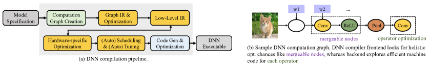
Figure 1: The high-level workflow of DL compilation.

Extracting DNN models from executables can boost many security applications, including adversarial example generation, training data inference, legacy DNN model reuse, migration, and patching. In contrast, existing model-extraction attacks, whether based on side channels [46, 30, 104, 45, 116, 105] or local retraining [79, 76, 94, 78], assume specific attack environments or can leak only parts of DNN models with low accuracy or high overhead.

We propose BTD, a decompiler for DNN executables. Given a (stripped) executable compiled from a DNN model, we propose a three-step approach for full recovery of DNN operators, network topology, dimensions, and parameters. BTD conducts representation learning over disassembler-emitted assembly code to classify assembly functions as DNN operators, such as convolution layers (Conv). Dynamic analysis is then used to chain DNN operators together, thus recovering their topological connectivity. To further recover dimensions and parameters of certain DNN operators (e.g., Conv), we launch trace-based symbolic execution to generate symbolic constraints, primarily over floating-point-related computations. The human-readable symbolic constraints denote semantics of corresponding DNN operators that are invariant across different compilation settings. Experienced DL experts can infer higher-level information about operators (e.g., dimensions, the memory layout of parameters) by reading the constraints. Nevertheless, to deliver an automated pipeline, we then define patterns over symbolic constraints to automatically recover dimensions and memory layouts of parameters. We incorporate taint analysis to largely reduce the cost of symbolic execution which is more heavyweight.

BTD is comprehensive as it handles all DNN operators used in forming computer vision (CV) models in ONNX Zoo [77]. BTD  processes x86 executables, though its core technique is mostly platform-independent. Decompiling executables on other architectures requires vendor support for reverse engineering toolchains first. We also find that DNN “executables” on some other architectures are not in standalone executable formats. See the last paragraph of Sec. 2 for the significance of decompiling x86 DNN executables, and see Sec. 8 for discussions on cross-platform support.

BTD was evaluated by decompiling 64-bit x86 executables emitted by eight versions of three production DL compilers, TVM [22], Glow [85], NNFusion [64], which are developed by Amazon, Facebook, and Microsoft, respectively. These compilers enable full optimizations during our evaluation. BTD is scalable to recover DNN models from 65 DNN executables, including nearly 3 million instructions, in 60 hours with negligible errors. BTD, in particular, can recover over 100 million parameters from VGG, a large DNN model, with an error rate of less than 0.1% (for TVM-emitted executable) or none (for Glow-emitted executable). Moreover, to demonstrate BTD’s correctness, we rebuild decompiled model specifications with PyTorch. The results show that almost all decompiled DNN models can be recompiled into new executables that behave identically to the reference executables. We further demonstrate that BTD, by decompiling executables into DNN models, can boost two attacks, adversarial example generation and knowledge stealing. We also migrate decompiled x86 DNN executables to GPUs, and discuss limits and potential future works. In summary, we contribute the following:

• This paper, for the first time, advocates for reverse engineering DNN executables. BTD accepts as input (stripped) executables generated by production DL compilers and outputs complete model specifications. BTD can be used to aid in the comprehension, migration, hardening, and exploitation of DNN executables.

• BTD features a three-step approach to recovering high-level DNN models. It incorporates various design principles and techniques to deliver an effective pipeline.

• We evaluate BTD against executables compiled from large-scale DNN models using production DL compilers. BTD achieves high accuracy in recovering (nearly) full specifications of complex DNN models. We also demonstrate how common attacks are boosted by BTD.

2 Preliminary

Fig. 1(a) depicts DNN model compilation. DNN compilation can be divided into two phases [58], with each phase manipulates one or several intermediate representations (IR).

Computation Graph. DL compiler inputs are typically high-level model descriptions exported from DL frameworks like PyTorch [80]. DNN models are typically represented as computation graphs in DL frameworks. Fig. 1(b) shows a simple graph of a multilayer convolutional neural network (CNN). These graphs are usually high-level, with limited connections to hardware. DL frameworks export computation graphs often in ONNX format [6] as DL compiler inputs.

Frontend: Graph IRs and Optimizations. DL compilers typically first convert DNN computation graphs into graph IRs. Hardware-independent graph IRs define graph structure. Network topology and layer dimensions encoded in graph IRs can aid graph- and node-level optimizations including operator fusion, static memory planning, and layout transformation [22, 85]. For instance, operator fusions and constant folding are used to identify mergeable nodes in graph IRs after precomputing statically-determinable components. Graph IRs specify high-level inputs and outputs of each operator, but do not restrict how each operator is implemented.

Backend: Low-Level IRs and Optimizations. Hardware-specific low-level IRs are generated from graph IRs. Instead of translating graph IRs directly into standard IRs like LLVM IR [55], low-level IRs are employed as an intermediary step for customized optimizations using prior knowledge of DL models and hardware characteristics. Graph IR operators can be converted into low-level linear algebra operators [85]. For example, a fully connected (FC) operator can be represented as matrix multiplication followed by addition. Such representations alleviate the hurdles of directly supporting many high-level operators on each hardware target. Instead, translation to a new hardware target only needs the support of low-level linear algebra operators. Low-level IRs are usually memory related. Hence, optimizations at this step can include hardware intrinsic mapping, memory allocation, loop-related optimizations, and parallelization [84, 17, 110, 22].

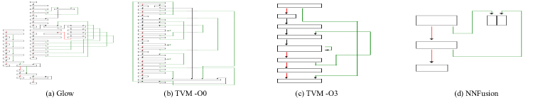
Figure 2: Compare CFGs of a Conv operator in VGG16 compiled by different DL compilers. TVM refers to enabling no optimization as “-O0” while enabling full optimizations as “-O3”. Glow and NNFusion by default apply full optimizations.

Backend: Scheduling and Tuning. Policies mapping an operator to low-level code are called schedules. A compiler backend often searches a vast combinatorial scheduling space for optimal parameter settings like loop unrolling factors. Halide [84] introduces a scheduling language with manual and automated schedule optimization primitives. Recent works explore launching auto scheduling and tuning to enhance optimization [12, 97, 70, 23, 22, 113, 114]. These methods alleviate manual efforts to decide schedules and optimal parameters.

Backend: Code Gen. Low-level IRs are compiled to generate code for different hardware targets like CPUs and GPUs. When generating machine code, a DNN operator (or several fused operators) is typically compiled into an individual assembly function. Low-level IRs can be converted into mature tool-chains IRs like LLVM or CUDA IR [73] to explore hardware-specific optimizations. For instance, Glow [85] can perform fine-grained loop-oriented optimizations in LLVM IR. DL compilers like TVM and Glow compile optimized IR code into standalone executables. Kernel libraries can be used by DL compilers NNFusion [64] and XLA [95] to statically link with DNN executables. Decompiling executables statically linked with kernel libraries are much easier: such executables contain many wrappers toward kernel libraries. These wrappers (e.g., a trampoline to the Conv implementation in kernel libraries) can be used to infer DNN models. This work mainly focuses on decompiling “self-contained” executables emitted by TVM and Glow, given their importance and difficulty. For completeness, we demonstrate decompiling NNFusion-emitted executables in Sec. 4.4.

Real-World Significance of DL Compilers. DL compilers offer systematic optimization to improve DNN model adoption. Though many DNN models to date are deployed using DL frameworks like Tensorflow, DL compilers cannot be disregarded as a growing trend. Edge devices and low-power processors suppliers are incorporating DL compilers into their applications to reap the benefits of DNN models [75, 48, 83, 74]. Cloud service providers like Amazon and Google include DL compilers into their DL services to boost performance [14, 101]. Amazon uses DL compilers to compile DNN models on Intel x86 CPUs [61, 49]. Facebook deploys Glow-compiled DNN models on Intel CPUs [69]. Overall, DL compilers are increasingly vital to boost DL on Intel CPUs, embedded devices, and other heterogeneous hardware backends. We design BTD, a decompiler for Intel x86 DNN executables. We show how BTD can accelerate common DNN attacks (Appendix D) and migrate DNN executables to GPUs (Sec. 8). Sec. 8 explains why BTD does not decompile executables on GPUs/accelerators. GPU/accelerator platforms lack disassemblers/dynamic instrumentation infrastructures, and the DL compiler support for GPU platforms is immature (e.g., cannot generate standalone executables).

3 Decompiling DNN Executables

Definition. BTD decompiles DL executables to recover DNN high-level specifications. The full specifications include: DNN operators (e.g., ReLU, Pooling, and Conv) and their topological connectivity, dimensions of each DNN operator, such as #channels in Conv, and parameters of each DNN operator, such as weights and biases, which are important configurations learned during model training. Sec. 4 details BTD’s processes to recover each component.

Query-Based Model Extraction. Given a (remote) DNN model with obscure specifications, adversaries can continuously feed inputs $x$ to the model and collect its prediction outputs $y$. This way, adversaries can gradually assemble a training dataset $(x,y)$ to train a local model [96, 79].

This approach may have the following challenges: 1) for a DNN executable without prior knowledge of its functionality, it is unclear how to prepare inputs $x$ aligned with its normal inputs; 2) even if the functionality is known, it may still be challenging to prepare a non-trivial collection of $x$ for models trained on private data (e.g., medical images); 3) local retraining may require rich hardware and is costly; and 4) existing query-based model extraction generally requires prior knowledge of model architectures and dimensions [79]. In contrast, BTD only requires a valid input. For instance, a meaningless image is sufficient to decompile executables of CV models. Also, according to the notation in Definition, local retraining assumes + as prior knowledge, whereas BTD fully recovers + + from DNN executables.

Model Extraction via Side Channels. Architectural-level hints (e.g., side channels) leaked during model inference can be used for model extraction [46, 30, 104, 45, 116, 105]. These works primarily recover high-level model architecture, which are or + according to our notation in Definition. In contrast, BTD statically recovers and then dynamically recovers + from DNN executables (but coverage is not an issue; see Sec. 4.2 for clarification). Sec. 9 further compares BTD with prior model extraction works.

Comparison with C/C++ Decompilation. BTD is different from C/C++ decompilers. C/C++ decompilation takes executable and recovers C/C++ code that is visually similar to the original source code. Contrarily, we explore decompiling DNN executables to recover original DNN models. The main differences and common challenges are summarized below.

Statements vs. Higher-Level Semantics: Software decompilation, holistically speaking, line-by-line translates machine instructions into C/C++ statements. In contrast, BTD recovers higher-level model specifications from machine instructions. This difference clarifies that a C decompiler is not sufficient for decompilation of DNN executables.

Common Uncertainty: There is no fixed mapping between C/C++ statements and assembly instructions. Compilers may generate distinct low-level code for the same source statements. Therefore, C/C++ decompilers extensively use heuristics/patterns when mapping assembly code back to source code. Likewise, DL compilers may adopt different optimizations for compiling the same DNN operators. The compiled code may exhibit distinct syntactic forms. Nevertheless, the semantics of DNN operators are retained, and we extract the invariant semantics from the low-level instructions to infer the high-level model specifications. See Sec. 4.3 for details.

End Goal: C/C++ compilation prunes high-level program features, such as local variables, types, symbol tables, and high-level control structures. Software decompilation is fundamentally undecidable [25], and to date, decompiled C/C++ code mainly aids (human-based) analysis and comprehension, not recompilation. Generating “recompilable” C code is very challenging [99, 98, 32, 102]. In this regard, DNN compilation has comparable difficulty, as compilation and optimization discard information from DNN models (e.g., by fusing neighbor operators). BTD decompiles DNN executables into high-level DNN specifications, resulting in a functional executable after recompilation. Besides helping (human-based) comprehension, BTD boosts model reuse, migration, security hardening, and adversarial attacks. See case studies in Sec. 8 and Appendix D.

Opacity in DNN Executables. Fig. 2 compares VGG16 [89] executables compiled using three DL compilers. For simplicity, we only plot the control flow graphs (CFGs) of VGG16’s first Conv operator. These CFGs were extracted using IDA-Pro [41]. Although this Conv is only one of 41 nodes in VGG16, Glow compiles it into a dense CFG (Fig. 2(a)). Sec. 2 has introduced graph-level optimizations that selectively merge neighbor nodes. Comparing CFG generated by TVM -O0 (Fig. 2(b)) and by TVM -O3 (Fig. 2(c)), we find that optimizations (e.g., operator fusion) in TVM can make CFG more succinct. We also present CFGs emitted by NNFusion in Fig. 2(d): NNFusion-emitted executables are coupled with the Mlas [67] kernel library. This CFG depicts a simple trampoline to the Conv implementation in MlasGemm.

As in Fig. 2, different compilers and optimizations can result in complex and distinct machine code realizations. However, BTD is designed as a general approach for decompilation of executables compiled by these diverse settings.

Design Focus. Reverse engineering is generally sensitive to the underlying platforms and compilation toolchains. As the first piece of work in this field, BTD is designed to process common DNN models compiled by standard DL compilers. Under such conservative and practical settings, BTD delivers highly encouraging and accurate decompilation. Similarly, obfuscation can impede C/C++ decompilation [62]. Modern C/C++ decompilers are typically benchmarked on common software under standard compilation and optimization [102, 21, 16, 99], instead of extreme cases. We leave it as a future work to study decompiling obfuscated DL executables.

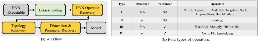
Figure 3: Decompilation workflow. Here “NA” in the “Dimension” column denotes an easy case where output dimension of an operator O equals to its input dimension and no other dimensions associated with O. We find that in non-trivial DNN, it is sufficient to decide O’s dimensions after propagating dimensions from other operators on the DNN computation graph.

4 Design

Decompiling DNN executables is challenging due to the mismatch between instruction-level semantics and high-level model specifications. DNN executables lack high-level information regarding operators, topologies, and dimensions. Therefore, decompiling DNN executables presents numerous reverse engineering hurdles, as it is difficult to deduce high-level model specifications from low-level instructions. We advocate DL decompilers to satisfy the following criteria:

R1 (Generalizability): Avoid brittle assumptions. Generalize across compilers, optimizations, and versions.

R2 (Correctness): Use effective, resilient methods and produce correct outputs.

R3 (Performance): Be efficient when necessary.

R4 (Automation): Avoid manual analysis and automate the decompilation process.

BTD delivers practical decompilation based on the invariant semantics of DNN operators that aims to meet all four criteria. Our intuition is simple: DL compilers generate distinct low-level code but retain operator high-level semantics, because DNN operators are generally defined in a clean and rigorous manner. Therefore, recovering operator semantics should facilitate decompilation generic across compilers and optimizations (R1). Besides, as invariant semantics reflect high-level information, e.g., operator types and dimensions, we can infer model abstractions accurately (R2).

Fig. 3(a) depicts the BTD workflow. Sec. 4.1 describes learning-based techniques for recognizing assembly functions as DNN operators like Conv. Given recovered DNN operators, we reconstruct the network topology using dynamic analysis (Sec. 4.2). We then use trace-based symbolic execution to extract operator semantics from assembly code and then recover dimensions and parameters with semantics-based patterns (Sec. 4.3.2). Some operators are too costly for symbolic execution to analyze. We use taint analysis to keep only tainted sub-traces for more expensive symbolic execution to analyze (R3), as noted in Sec. 4.3.1. BTD is an end-to-end, fully automated DNN decompiler (R4). BTD produces model specifications that behave identically to original models, whose focus and addressed challenges are distinct from C/C++ decompilation. BTD does not guarantee 100% correct outputs. In Sec. 5, we discuss procedures users can follow to fix errors.

Dimensions and parameters configure DNN operators. We show representative cases in Fig. 3(b). Type I operators, including activation functions like ReLU and element-wise arithmetic operators, do not ship with parameters; recovering their dimensions is trivial, as clarified in the caption of Fig. 3. Type II and III operators require dimensions or parameters, such as Pooling’s stride $S$ and kernel size $K$. In addition to simple arithmetic operators, BiasAdd involves bias $B$, as extra parameters. Type IV operators require both parameters and dimensions. These operators form most DNN models. Sec. 7.1 empirically demonstrates “comprehensivness” of our study.

BTD recovers dimensions/parameters of all DNN operators used by CV models in ONNX Zoo (see Sec. 7.1). Due to limited space, Sec. 4.3 only discusses decompiling the most challenging operator, Conv. The core techniques explained in Sec. 4.3 are utilized to decompile other DNN operators. However, other operators may use different (but simpler) patterns. Appendix C lists other operator patterns. We further discuss the extensibility of BTD in Sec. 7.3.

Disassembling and Function Recovery. BTD targets 64-bit x86 executables. Cross-platform support is discussed in Sec. 8. BTD supports stripped executables without symbol or debug information. We assume that DNN executables can be first flawlessly disassembled with assembly functions recovered. According to our observation, obstacles that can undermine disassembly and function recovery in x86 executables, e.g., instruction overlapping and embedded data [32], are not found in even highly-optimized DNN executables. We use a commercial decompiler, IDA-Pro [41] (ver. 7.5), to maximize confidence in the credibility of our results.

Compilation Provenance. Given a DNN executable $e$, compilation provenance include: 1) which DL compiler is used, and 2) whether $e$ is compiled with full optimization -O3 or no optimization -O0. Since some DNN operators (e.g., type IV in Fig. 3(b)) in $e$ are highly optimized when compiled, the compilation provenance can be inferred automatically by analyzing patterns over sequences of x86 instructions derived from $e$. We extend our learning-based method from Sec. 4.1 to predict compilation provenance from assembly code. Our evaluation of over all CV models in ONNX Zoo finds no errors. Overall, we assume that compilation provenance is known to BTD. Therefore, some patterns can be designed separately for Glow- and TVM-emitted executables; see details in Appendix C. To show $e$’s decompilation is flawless, we must recompile decompiled DNN models with the same provenance (see Sec. 7.1.4). Using different compilation provenances may induce (small) numerical accuracy discrepancies and is undesirable.

This section focuses on decompilation of self-contained DNN executables compiled by TVM and Glow. Decompilation of NNFusion-emitted executables is easier because of its distinct code generation paradigm. We discuss decompiling NNFusion-emitted executables in Sec. 4.4.

4.1 DNN Operator Recovery

As introduced in Sec. 2, one or a few fused DNN operators are compiled into an assembly function. We train a neural model to map assembly functions to DNN operators. Recent works perform representation learning by treating x86 opcodes as natural language tokens [28, 81, 108, 29, 59]. These works help comprehend x86 assembly code and assist downstream tasks like matching similar code. Instead of defining explicit patterns over x86 opcodes to infer DNN operators (which could be tedious and need manual efforts), we use representation learning and treat x86 opcodes as language tokens.

Atomic OPs. Launching representation learning directly over x86 opcodes syntax can result in poor learning quality. Due to x86 instructions’ flexibility, opcodes with (nearly) identical semantics may have distinct syntactic forms, e.g., vmulps and mulps denoting multiply over floating numbers of different sizes. Rare words machine translation [88] are recently advanced from the observation that natural language words can be divided into atomic units. Translators can use atomic units to translate rare words. Accordingly, we define atomic OPs over x86 opcodes: an atomic OP represents an atomic and indivisible unit of an x86 opcode. Each opcode is thus split into atomic OPs. While a DNN operator could be compiled into various x86 opcode sequences, induced atomic OP sequences can better reflect “semantics” in a noisy-resilient way.

Dividing Opcodes into Atomic OPs. As a common approach, we segment opcodes using Byte Pair Encoding (BPE) [35]. BPE iteratively replaces the most frequent consecutive bytes in a sequence with a single, unused byte. We split each opcode into a sequence of characters and counted consecutive characters to find the most frequent ones. BPE iterates until the opcodes of all atomic OPs have been merged. For instance, opcodes vmulps and mulps are first split into “v m u l p s” and “m u l p s”, and an atomic OP mulps is eventually extracted.

Learning over Atomic OPs. We train a neural identifier model with a sequence of atomic OPs from an assembly function as inputs. This model outputs a 1D vector with $N$ dimensions ($N$ is the total number of unique DNN operators), where multiple “1” in the vector implies that this assembly function represents several fused DNN operators. All “0” in the vector implies this function may be a DL compiler-inserted utility function (e.g., for memory management). The order of fused operators is represented in symbolic constraints extracted in Sec. 4.3. Thus, predicted operator labels and network topology will be refined after symbolic execution. Our model’s frontend learns a neural embedding for each atomic OP and then embeds a function’s entire atomic OP sequence. The order of atomic OPs is found to be vital in prediction. Therefore, we preserve the order of collected atomic OPs within the assembly function. We encode orders with LSTM [43] (see Sec. 5) and enhance learning with neural attention [18].

From Operators to Compilation Provenance. As noted in Sec. 4, our decompilation pipeline requires compilation provenance. We extend the model presented in this section to recover compilation provenance. The extended model predicts compilation provenance using embeddings of all functions in an executable as its input (function embeddings have been generated above). We clarify this task is generally simple; humans can easily distinguish assembly functions in executables from different compilation provenances.

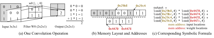
Figure 4: Launching trace-based symbolic execution (SE) to infer dimensions and localize parameters for Conv operators.

4.2 DNN Network Topology Recovery

Recovering DNN network topology is straightforward, regardless of underlying operator semantics. DNN operators are chained into a computation graph. Generally, a DNN operator has a fixed number of inputs and outputs [9]. According to our observation, DL compilers compile DNN operators into assembly functions and pass inputs and outputs as memory pointers through function arguments. We use Intel Pin [63], a dynamic instrumentation tool, to hook every callsite. During runtime, we record the memory addresses of inputs/outputs passed to callsites and connect two operators if the successor’s inputs match the predecessor’s outputs.

We do not rely on any compiler-specific assumptions like function signatures. This step is independent of later steps and only uses shallow information readily available in binaries. In case the inputs and outputs are passed differently (e.g., not using pointers) in further compiler implementation changes, we envision updating the instrumented code accordingly without much engineering effort required. Also, we clarify that this dynamic analysis is not limited by “coverage”. We do not require “semantically meaningful” inputs (not like a query-based model extraction [96, 79]), just a format-valid input to record how each operator in the executable accesses memory. One format-valid, trivial (meaningless) input can achieve 100% coverage. Besides, whether a model accepts images or text as its valid inputs is easy to determine.

4.3 Dimension and Parameter Recovery

As in Fig. 3, certain complex DNN operators are configured with dimensions and parameters. This section details solutions to recover parameters/dimensions. To present a comprehensive working example, we use Conv, the most complex operator in our dataset, to introduce our solutions. Nonetheless, our solutions are general enough to cover all operators in CV models of ONNX Zoo (see Sec. 7.1) and can be extended to support more operators with trivial effort (see Sec. 7.3).

Fig. 4(a) shows the input, the kernel, and the output of a simple Conv computation. Suppose no optimization is applied, we present the memory layout of Conv in Fig. 4(b). Inputs and parameters are typically stored separately in memory, whereas neighbor input/parameter elements are stored contiguously. Fig. 4(c) reports the invariant semantics of the Conv operator in Fig. 4(a), in the form of a symbolic constraint.

General Workflow. Recovering dimensions and parameters has several tasks. The essential of our solution is to summarize operator invariant semantics with symbolic execution. We first log execution traces and use taint analysis to shorten the traces. We then use symbolic execution to summarize the input-output constraint of each assembly function, infer dimensions using patterns defined over constraints, and further extract parameters. We detail each task below.

4.3.1 Trace Logging and Taint Analysis

Execution trace-based analysis is ideal to analyze DNN executables, because any non-trivial inputs achieve full coverage. We use Intel Pin [63] to log the execution trace of an operator’s assembly function. Complex DNN operators like Conv are computation intensive, and a single Conv execution trace can reach to hundreds of gigabytes. Pin takes several hours to log one trace. Nonetheless, Conv is generally compiled into nested loops. Hence, analyzing a subtrace containing one iteration of the outermost loop is sufficient (as long as a complete calculation of an output element is reflected in this subtrace).

Taint Analysis. The subtrace can still be up to several gigabytes in size. We further use backward taint analysis [86, 51] to rule out instructions that are not involved in computing outputs. We mark this operator’s output elements as taint sources and analyze the trace backward. Our taint propagation is straightforward to track data dependency [86, 51, 100]. Trace logging records each instruction’s execution context, including concrete memory address values. Thus, for each memory access during taint propagation, we compute concrete addresses to taint/untaint memory cells accordingly.

4.3.2 Symbolic Execution (SE)

We launch SE over tainted x86 instructions. While existing symbolic execution tools do not support pervasive SSE instructions in DNN executables, we reimplement a trace-based SE engine that models all SSE floating-point computations encountered in tainted traces. We ignore irrelevant semantics like CPU flags. As with taint analysis, symbolic pointers are computed using concrete values. For instance, movss xmm1, dword ptr [rcx] will load floating numbers from memory pointed by rcx. Given that dword denotes 4 bytes, if rcx is 0x29b8, we create (0x29b8, 4) as xmm1’s symbolic value while the upper 16-4 bytes are reset to zero. After performing SE on tainted trace, we get a (simplified) symbolic constraint as in Fig. 4(c), which shows how inputs and parameters in memory (see Fig. 4(b)) are used to computing an output.

Identifying Memory Layouts. To determine if each address in the symbolic constraint points to inputs or parameters, we form a once-for-all configuration that records the meaning of each argument (inputs or parameters) of the corresponding assembly function for different operators (see Appendix B). We can collect and identify inputs and parameters’ memory addresses by querying the configuration. For the constraint in Fig. 4(c), we will identify memory addresses and classify them into weights (marked in red) and inputs (marked in yellow). Furthermore, by logging and identifying all memory addresses accessed during an operator’s computation, we can cluster all addresses of the same parameter to scope that parameter’s memory region (i.e., the starting address and size).

4.3.3 Dimension Recovery

For reverse engineering, heuristic are hardly avoidable [99, 98]. We now present patterns defined over the extracted constraints, which enable recovering dimensions and parameter layouts. Without compromising generality, we mainly introduce patterns we use to recover Conv operator dimensions and layouts. Other operators in our dataset can be covered smoothly with simpler patterns, as we stated in Sec. 4.3.

Kernel Size $K$, Input Channel $I_{C}$, Zero Padding $P$. Consider Fig. 4(c), given the relative offsets of four marked input memory addresses are [0, 4, 12, 16], we can infer the kernel shape as $2\times 2$ (the continuous sequence has length 2), indicating that $K=2$. Further, we calculate #input channels $I_{C}=\frac{4}{2\times 2}=1$, as to compute one output element, we recognize four inputs (which belong to one input channel) in the symbolic constraint. Also, considering the memory layout in figure b, it should be easy to infer that “12” denotes the first element from the next row (element at row 3, column 2). Hence, we can compute the shape of the input matrix as $\frac{12}{4}=3$ where $4$ denotes the size of one floating number on 64-bit x86 platforms. The input shape is therefore $3\times 3$. As the network topology has been recovered in Sec. 4.2, we compare the output of the prior operator with the input of this Conv to decide zero padding $P$. Suppose the output shape of the prior operator is $1\times 1$, $P$ is decided as $\frac{3-2}{2}=1$.

Output Channels $O_{C}$. To infer $O_{C}$, we re-run Pin and log all accessed memory locations when executing Conv. Since we do not need to log every instruction and its associated context (which involves lots of string conversions and I/Os), Pin runs much faster than being used to log execution traces in Sec. 4.3.1. We then re-launch the analysis detailed in Identifying Memory Layouts to identify all addresses belonging to weights and then determine the size of the memory region that stores weights, which implies the size of weights. Let the memory region size be $M_{w}$, $O_{C}$ can be computed as $\frac{M_{w}}{I_{C}\times K\times K}$.

Stride $S$. Let the input (output) height be $IH_{i}$ ($OH_{i}$), we compute stride $S$ using the following dimension constraint:

$$OH_{i}=[(IH_{i}+2P-K)/S]+1$$

The memory region size $M_{i}$ of Conv inputs can be decided in the same way as deciding $M_{w}$. Hence, the input height can be computed as $IH_{i}=\sqrt{\frac{M_{i}}{I_{c}}}$. Similarly, we can compute $OH_{i}$ as $\sqrt{\frac{M_{o}}{O_{c}}}$, where $M_{o}$ is the memory region size of Conv outputs. Stride $S$ is thus computed using the constraint above.

In sum, BTD extracts a series of facts based on the symbolic constraint and runtime information of DNN executables, including 1) the memory regions size of inputs, outputs, and parameters, 2) the relative offsets of the input memory addresses, 3) the relative offsets of the parameter memory addresses, and 4) the number of specific arithmetic operations inside a symbolic constraint. Lacking any of these cannot fully recover a (complex) DNN operator. Nevertheless, since these facts are consistantly presented in DNN executables generated by different DL compilers, our dimension recovery techniques are generic across compilers and optimizations. See Appendix C for handling other operators (in the same procedure) and Sec. 7.2 for the generalization evaluation.

4.3.4 Recover Parameters

Recovering parameters requires to identify their starting addresses and memory layouts. As clarified in #Output Channels $O_{C}$, we identify memory region $M_{w}$ that stores parameters. We then use Pin to dump parameters to disk at runtime. With recovered dimensions and dumped parameters in data bytes, we can recover well-formed parameters. Operators may have multiple parameters, and more than one pointers to distinct parameters may appear in the assembly function arguments (see Appendix B for function interfaces of operators). Each pointer’s parameter is recovered separately.

Handling Compiler Optimizations. Fig. 4(b) depicts a Conv’s memory layout. However, compilers may optimize Conv to reduce runtime cost. Both TVM and Glow may perform layout alteration optimizations to take advantage of SSE parallelism by reading 4 (or 8) floating numbers from contiguous memory into one register. These floating numbers can be computed with one SSE instruction (optimized memory layout is depicted in Sec. 7.1.6). These optimizations modify Conv’s standard memory layout, impeding parameter recovery. Similar to dimension inference, we use patterns to identify optimized layouts. We detail patterns in Appendix F. In short, BTD is nearly flawless; see discussion in Sec. 7.1.6.

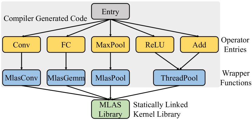
Figure 5: Holistic view of call graph of binary code generated by NNFusion.

4.4 Executables Emitted by NNFusion

The procedure described in Sec. 4 decompiles self-contained DNN executables — outputs of the dominant compilers TVM and Glow. As introduced in Sec. 2, some DL compilers, including NNFusion [64] and XLA [95], generate executables statically linked with kernel libraries. It is easier to decompile NNFusion- and XLA-emitted executables since they contain wrapper functions to invoke target operator implementations in kernel libraries. We easily determine DNN operator types by matching those wrapper functions. During runtime, we use Pin to recover network topology and intercept data sent via wrappers. The intercepted data include dimensions (in integers) and pointers to parameters. We use obtained dimensions/pointers to load parameters from the memory. Sec. 7.1.5 assesses BTD using NNFusion-compiled executables.

Fig. 5 depicts a high-level workflow of DNN executable compiled by NNFusion, where a set of distinguishable wrapper functions are deployed as trampolines to invoke target DNN operator implementations in Mlas [67], high-speed linear algebra library. Since code in kernel libraries is constant from model to model, we can easily distinguish between the corresponding wrapper functions by the functions in the libraries being called. Therefore, it becomes much easier to recover the DNN structure, as we can decide the DNN operator types via statically pattern matching wrapper functions (e.g., MlasGemm). More specifically, we envision that well-developed code similarity techniques [28, 29] or manually defined patterns could be used to identify kernel library functions smoothly. While this work primarily focuses on decompiling more challenging code generation patterns (as elaborated in Sec. 2), given such patterns are adopted by industrial-strength DNN compilers, TVM [22] and Glow [85], we only empirically demonstrate the feasibility of decompiling NNFusion executables in Sec. 7.1.5. Executables compiled by XLA can be processed similarly.

5 Implementation

BTD is primarily written in Python with about 11K LOC. Our Pin plugins contain about 3.1K C++ code. The current implementation decompiles 64-bit executables in the ELF format on x86 platforms, See discussion on cross-platform support in Sec. 8. We use LSTM for DNN operators inference in an “out-of-the-box” manner to deal with distinct optimized low-level code of the same type of operator resulting from different dimensions. The model is a one-layer LSTM [43] whose hidden dimension is 128. The LSTM is implemented using PyTorch [80], with CUDA 10.0 [72] and cuDNN [24].

6 Usage & Error Fixing

BTD offers an end-to-end, automated decompilation. All tasks of Fig. 3(a) require no human intervention. However, decompilation is inherently challenging, and BTD may make mistakes. This section first explains how a user use BTD in practice, and then discuss error fixing.

Usage. Given a DNN executable, a user first disassembles it (e.g., using IDA-Pro) and recovers all assembly functions. The user also need to provide a format-valid input of this executable for use. Next, as an end-to-end procedure, BTD predicts compilation provenance and each disassembly function’s operator type. BTD then launches the network topology recovery before conducting symbolic execution and recovering dimensions and parameters for each operator, as explained in Sec. 4. Note that at this step, BTD uses a set of error detection rules (see below) to detect and fix potential errors. Decompilation process is then re-invoked if errors are fixed. If the error cannot be resolved, human intervention is required. The user needs to read and understand the symbolic constraints to fix the error. Human comprehension at this step is the only uncertain but necessary step of the decompilation if complex errors occur. Finally, the user can rebuild the model using the recovered model specification on DL frameworks like PyTorch.

Error Fixing. To augment BTD’s decompilation pipeline, we provide a set of rules based on the basic knowledge of ML models, whose violation uncovers decompilation errors. Some rules have error-fixing actions, but not all errors can be fixed in an automated manner. In that case, the user can inspect and fix those errors manually. Also, the user may extend the rules based on their observation and experience of ML models. Currently, we have six error detection rules, of which Rules 1–4 have follow-up automated fixing actions, while Rules 5–6 require human intervention for error fixing:

1. Dimensions of Conv operators must be integers. Otherwise, BTD reports an error and instead uses input/output of predecessor/successor operators to form the dimensions; see a relevant case study in Appendix E.

2. Inputs of Add operators must be other operators’ outputs. If not, BTD infers this operator type as BiasAdd.

3. The Split operator’s output memory region size should be smaller than its input memory region size. If not, BTD instead infers this operator type as Concatenate.

4. The symbolic constraint of an operator with ReLU label (e.g., “Conv+ReLU”) must contain a “max” operation. If not, BTD fixes its inferred operator type by removing the “ReLU” label (e.g., “Conv+ReLU” $\rightarrow$ “Conv”).

5. If operator inference model’s confidence score is below 80%, and no error is detected by Rules 2-4, BTD throws an error and requires human intervention.

6. An operator’s input shape must match its predecessor’s output shape. Otherwise, BTD throws an error and requires human intervention.

Conceptually, Rule 1 and 6 validate dimension inference, whereas Rules 2–5 validate operator inference results. Rules 2–5 are designed based on observations of our manual exploration, not failed cases when inferring test models.

Table 1: Compilers evaluated in our study.

Tool Name	Publication	Developer	Version (git commit)
TVM [22]	OSDI ’18	Amazon	v0.7.0
			v0.8.0
			v0.9.dev
Glow [85]	arXiv	Facebook	2020 (07a82bd9fe97dfd)
			2021 (97835cec670bd2f)
			2022 (793fec7fb0269db)
NNFusion [64]	OSDI ’20	Microsoft	v0.2
			v0.3

Table 2: Statistics of DNN models and their compiled executables evaluated in our study.

Model	#Parameters	#Operators	TVM -O0		TVM -O3		Glow -O3
			Avg. #Inst.	Avg. #Func.	Avg. #Inst.	Avg. #Func.	Avg. #Inst.	Avg. #Func.
Resnet18 [39]	11,703,912	69	49,762	281	61,002	204	11,108	39
VGG16 [89]	138,357,544	41	40,205	215	41,750	185	5,729	33
FastText [20]	2,500,101	3	9,867	142	7,477	131	405	14
Inception [92]	6,998,552	105	121,481	615	74,992	356	30,452	112
Shufflenet [111]	2,294,784	152	56,147	407	34,637	228	33,537	59
Mobilenet [44]	3,487,816	89	69,903	363	46,214	228	37,331	52
Efficientnet [93]	12,966,032	216	89,772	546	49,285	244	13,749	67

7 Evaluation

In this section, we evaluate BTD by exploring the following four research questions (RQs) below:

RQ1 (Comprehensiveness and Correctness): Is BTD comprehensive and correct to process all operators used in common DL models compiled with different compilers and optimization options?

RQ2 (Robustness): Is BTD robust to survive frequent DL compiler implementation changes?

RQ3 (Extensibility): Can BTD be easily extended to support new operators and models? What efforts are needed?

RQ4 (Error Fixing): How does BTD handle decompilation errors?

We evaluated BTD with seven real-world CV models and an NLP model compiled with eight versions of compilers to provide a comprehensive evaluation. BTD can produce correct model specifications on 59 of 65 DNN executables, and experienced users can quickly fix 3 of 6 remaining errors. Nevertheless, we recognize that some errors cannot be easily fixed by normal users. In the evaluation, we only use ground truths to verify the correctness of decompilation results. BTD is designed to cope with real-world settings and does not rely on any ground truth. Setup and results are below.

Compilers. Table 1 lists compilers we used. We select eight versions of three state-of-the-art DL compilers. Glow does not have a release yet, so we use three versions that are at least six months apart. Glow and NNFusion only generate fully-optimized executables, but TVM can be configured to use different optimization levels. Therefore, we use TVM with no and full optimizations to build two sets of executables, while using Glow and NNFusion with default settings. All models are compiled into 64-bit x86 executables. Sec. 2 and Sec. 4.4 describe NNFusion’s distinct code generation paradigm. We study decompiling NNFusion-emitted executables in Sec. 7.1.5. Other evaluations in this section use TVM- and Glow-compiled executables.

Test Data. Table 2 lists all evaluated DNN models. All these models, except FasstText, are extensively used in CV tasks. NNFusion can only compile its own shipped VGG11. Our large-scale dataset includes a total of 675 operators and more than 178 million parameters. Note that these operators have covered all types of DNN operators used in the CV models in ONNX Zoo. FastText is a common NLP model that contains Embedding, FC, and Pooling. Embedding is a frequently-used DNN operator in NLP models that encodes text into embedding vectors. Since Embedding is not included in the training dataset, we manually label functions in FastText.

These ONNX files are compiled with TVM and Glow and then disassembled with IDA-Pro. Table 2 presents assembly code statistics. In general, one (or several fused) operator corresponds to one TVM/Glow compiled assembly function. Besides, TVM and Glow will add utility functions (e.g., for memory management). Table 2 reports average statistics across different versions of DL compilers.

Training the DNN Operator Identifier. To train the DNN operator identifier, we form a dataset using all 15 image classification models (we have excluded image classification models that are in our test dataset) provided by ONNX Zoo [77], such as AlexNet [53] and Inception [91]. These models are all commonly-used in daily DL tasks. To prepare training data, we use TVM and Glow to compile the ONNX files of these models into executables. DL compilers can be configured to output rich meta information during compilation, which describes the topology of the compiled model and dimensions/types information of operators. We take this meta information as the ground truth.

Processing Time. All experiments run on Intel Xeon CPU E5-2678 with 256GB RAM and an Nvidia RTX 2080 GPU. Generally, processing time is not a concern for BTD. Training operator identifier described in Sec. 4.1 takes less than one hour. The total operator identification time is about one second. Recovering DNN network structures (Sec. 4.2) requires only a few seconds since DNN executables are all lightweight instrumented in this task. Taint analysis can take from minutes to hours, depending on model size. Symbolic execution and parameter extraction usually take several minutes. Appendix A report details of processing time.

Boosting DNN Attacks. BTD extracts high-level model specifications from executables, allowing attackers to carry out white-box attacks toward the decompiled DNN models. In contrast, when attackers can only interact with DNN executables, attackers have to launch black-box attacks. With BTD, we demonstrate two attacks: adversarial example (AE) generation [71] and knowledge stealing [42] in a white-box setting. The results suggest that the white-box attacks enabled by BTD are much more powerful than the black-box settings. BTD enables recovering $151.4\times$ more AEs than the blackbox setting within 20 minutes, and the knowledge stolen from white-box models are of much higher quality than from the black-box executables; see details in Appendix D.

7.1 RQ1: Correctness and Comprehensiveness

This section answers RQ1. Our evaluation dataset contains landmark CV models and a common NLP model listed in Table 2. These CV models contains all kinds of operators used by CV models in ONNX Zoo. We first present an in-depth evaluation of decompiling CV models, assessing the correctness and comprehensiveness of BTD’s technical pipeline over all included DNN operators. We then discuss the comprehensiveness over NLP and audio processing models.

Table 3: Average accuracy of DNN operator inference.

Model	Glow			TVM -O0			TVM -O3
	2020	2021	2022	v0.7	v0.8	v0.9.dev	v0.7	v0.8	v0.9.dev
ResNet18	100%	100%	100%	99.79%	99.84%	100%	98.15%	99.06%	99.69%
VGG16	100%	100%	100%	99.95%	99.79%	99.57%	99.75%	100%	100%
Inception	100%	100%	100%	99.98%	99.88%	99.98%	100%	100%	100%
ShuffleNet	100%	100%	100%	99.96%	99.82%	100%	99.62%	99.71%	99.31%
MobileNet	100%	100%	100%	99.35%	99.46%	99.40%	99.80%	100%	100%
EfficientNet	100%	100%	100%	99.65%	99.68%	99.59%	99.81%	99.91%	100%

7.1.1 Predicting DNN Operator Type

In our test dataset, Glow-compiled executables have 14 types of DNN operators and TVM-compiled executables have 30. As introduced in Sec. 4.1, our operator identifier outputs a 1D vector of 14 or 30 elements for each assembly function, where a “1” in $k$th element indicates that this function should be labeled to $k$th operator. We allow multiple “1”, because operators can be fused into one assembly function. As a result, DNN operator inference is performed as two-class classification tasks over 14 or 30 labels. DL compilers provide the ground truth (function labels). We report the overall accuracy in Table 3, where prediction of an function is correct, when the predicted label describes exactly the same operation as the ground truth label. We interpret the prediction as highly accurate. Particularly, we achieve 100% accuracy for all executables compiled by Glow. We check all errors in TVM and discuss the root causes as follows:

Data Bias. Conv is commonly used with a following ReLU for feature extraction. Given “Conv+ReLU” patterns are frequent in training data, a ConvAdd operator emitted by TVM -O3 is mislabeled as ConvAddReLU. In contrast, Dense is often used in the last few layers of DNN without ReLU. Therefore, when ReLU is fused with DenseAdd under TVM -O3, our model mislabels DenseAddReLU as DenseAdd. Unbalanced real-world training data causes these mislabels. Errors may be eliminated by post-checking if symbolic constraints indicating ReLU (i.e., containing “max”) exists.

Operators with Similar Assembly Code. In TVM generated code, BiasAdd can be predicted as Add, and vice versa. As expected, assembly code of these two operators are similar. Our identifier’s confidence scores when labeling such operators with similar assembly code are close to the decision boundary, i.e., 50%. However, for other cases, the confidence scores are all significantly higher. We thus use the error detection method introduced in Sec. 6 to detect such errors in the early stage. Rules 2–4 in Sec. 6 are sufficient to detect all operator labelling errors. Morevoer, after applying fixing actions associated with Rules 2–4, we get the correct results over all models, i.e., all results in Table 3 become 100%. Besides, Rule 6 in Sec. 6 will throw a warning and require human validation when confidence is lower than 80%.

Table 4: Parameter/dimension inference. Each column reports dimension inference accuracy/parameter inference accuracy. The complete data is available in Table 10.

Model	Glow	TVM -O0	TVM -O3
	(2020, 2021, 2022)	(v0.7, v0.8, v0.9.dev)	(v0.7, v0.8, v0.9.dev)
ResNet18	100%/100%	92.15%/99.37%	100%/99.37%

7.1.2 DNN Network Topology Recovery

Recovering network topology (Sec. 4.2) is straightforward and rapid. To validate correctness, we compare the recovered network topology with the reference DNN’s computation graph for executables compiled by TVM -O0. For all evaluated DNN models, the recovered network structure is fully consistent with the reference. As for executables compiled by TVM -O3 and Glow, optimizations can change the high-level graph view of models. Thus, it becomes difficult to compare the recovered topology with reference models. Nevertheless, we note that all these test cases are shown as flawless in the recompilation study (Sec. 7.1.4). Therefore, the correctness of topology recovery for optimized cases is validated.

7.1.3 Parameter and Dimension Recovery

Table 4 reports parameter/dimension recovery accuracy. We only list results for ResNet (as its recovery at this step has defects). Besides ResNet, the accuracies for all other models are 100%, and results are consistent across different compiler versions; see complete data in Table 10. Except for TVM -O0, it is difficult to compare the recovered dimensions/parameters with the reference due to compiler optimizations. Hence, #failures in Table 4 equals #dimensions or #parameters that need to be fixed before the recovered models can be compiled into executables showing identical behavior with the references. Some operator inference failures do not involve dimensions/parameters, and are thus not reflected in Table 4.

Overall, BTD can determine dimensions of different DNN operators with negligible errors over all settings. Four failures in ResNet18 (TVM -O0) are due to a Conv optimization (see Sec. 7.1.6), while all dimensions of ResNet18 (TVM -O3) are correctly recovered. Besides, despite huge volume of parameters in each model, the results are promising. BTD failed to recover about 73K parameters of an optimized Conv operator in ResNet18 (TVM -O3) due to its specially-optimized memory layout; see root causes in Sec. 7.1.6.

Table 5: Recompilation. “NA” means that some errors are not fixed, thus the rebuilt models manifest inconsistent behavior. See full results in Table 11.

Model	Glow	TVM -O0	TVM -O3
	(2020, 2021, 2022)	(v0.7, v0.8, v0.9.dev)	(v0.7, v0.8, v0.9.dev)
ResNet18	100%	100% (with fixing)	NA $\rightarrow$ 100%

7.1.4 Recompilation

Recompilation is an active field in reverse engineering, though recompiling decompiled C/C++ code is challenging [99, 32, 98, 102]. This section demonstrates the feasibility of recompiling decompiled DNN models. Recompilation requires a fully fledged decompilation, with the end results again being a functional executable exhibiting identical behavior with the reference. This demonstrates the feasibility of DNN model reuse, migration, and patching. To do so, we re-implement DNN models in PyTorch using recovered DNN models, then export models as ONNX files and compiled into DNN executables using the same compilation provenance.

It is not desirable to directly compare the recovered high-level model specifications with the reference model’s specifications: compilation and optimization inevitably change DNN model representation (e.g., fusing operators). Thereby inconsistency of two high-level specifications does not necessarily indicate a difference in model outputs. Instead, We compare recompiled and reference executables directly. Specifically, we compare the predicted labels and confidence scores yielded by recompiled and reference executables over every input from validation dataset. Two executables are deemed identical if labels and confidence scores are exactly identical or with only negligible floating-point precision loss. For image classification models, we randomly select 100 images from 100 different categories in ImageNet [27] to form a validation dataset. For FastText, we randomly crafted 50 inputs.

Table 5 reports the results (only including ResNet18 as its recompilation has defects). All recompiled models manifest identical behavior with references over all inputs in the validation dataset except ResNet. Errors in ResNet (TVM -O0) can be fixed automatically with error fixing rules (see Sec. 7.4), and we mark “100% (with fixing)”. BTD  fails to detect an error in recovering the parameter layout of a Conv in ResNet18 (TVM -O3); we mark it “NA”. To verify the correctness of the remaining recovered operators in this model, we manually fixed this error with ground truth and re-ran the recompilation study; this model also gets 100% correct outputs, marked as “NA $\rightarrow$ 100%” in Table 5. In this case, BTD does not produce the correct and directly usable model specification, and the manual fixing here is merely to prove that all remaining operators in ResNet18 are correctly decompiled.

We also measure the size and speed of recompiled and reference executables. We report that no noticeable changes can be observed comparing recompiled and original executables.

7.1.5 Decompiling NNFusion Outputs

As clarified in Sec. 4.4, decompiling executables emitted by NNFusion and XLA are much easier, as these executables are linked with kernel libraries. For completeness, we run an automated process to decompile executables emitted by NNFusion v0.2 and v0.3. NNFusion cannot compile VGG provided by ONNX Zoo. We thus compile the VGG11 model shipped by NNFusion. This VGG11 model is in the bytecode format, and we cannot directly compare the recovered DNN model with the reference. We therefore directly check recompilation correctness. When re-compiling the ONNX file of the decompiled model, NNFusion throws exceptions, which, to our knowledge, seems to be bugs. To verify the correctness, we instead implement VGG in PyTorch using recovered VGG descriptions. We follow the same step in Sec. 7.1.4 to validate the recovered model. Note that PyTorch and DNN executables may show negligible deviation between results, which, we believe is from numerical accuracy instead of errors. We set a threshold to allow 10^-4 difference in the outputs of VGG in PyTorch and in executable. All validation inputs are passed. Therefore, we conclude that decompilation is correct.

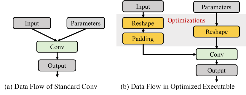
Figure 6: Reshapes inserted before Conv by TVM.

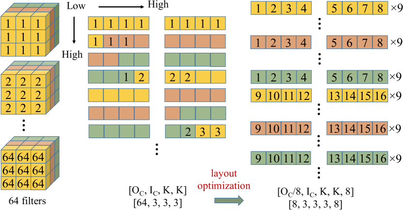
Figure 7: Layout optimization.

7.1.6 Root Cause Analysis

Besides errors due to mislabeled operators, two failures occurred when inferring parameters and dimensions. We now discuss the root causes.

Case One. All dimension/parameter recovery failures of ResNet (TVM -O0) are from one Conv operator. The failure is due to a Reshape operator inserted by TVM before Conv. Recall to infer dimensions of Conv (particularly the kernel shape $K$), we define patterns over offsets of kernel memory addresses (Sec. 4.3.3). However, to speed up program execution, TVM may add extra code to reshape the input at runtime before convolutional calculation, as shown in Fig. 6. In short, after optimization, the input addresses extracted over symbolic constraints no longer solely reflect elements in the Conv kernels, thus restraining our patterns.

Case Two. Another parameter recovery failure also roots in Conv compiled with TVM -O3. Fig. 7 presents the standard memory layout of a Conv which is denoted as $[O_{C},I_{c},K,K]$. While this layout can be flawlessly recovered by BTD, as mentioned in Sec. 4.3.4, DL compilers may alter memory layout of parameters to take advantage of SSE instructions. As shown in Fig. 7, the parameter layout can be converted into an optimized version which is denoted as $[O_{C}/A,I_{c},K,K,A]$. BTD can correctly infer memory layouts for 33 of 34 Conv operators optimized this way (see our patterns in Appendix F). Nevertheless, we still encounter one rare case where weights are not loaded in the order assumed in our patterns, which is likely due to TVM’s auto scheduling. This breaks our patterns to recover parameters. In contrast, while Glow also extensively uses this optimization, BTD can flawlessly recover parameters from all Conv operators optimized by Glow.

7.1.7 Other Models

Table 6: NLP models compilation results. “Crash” means compilers throw an exception and terminate. “Failed” means executable output is inconsistent with the input model. “Success” means the model is compiled correctly.

Model	Glow	Glow	TVM	TVM	NNFusion
	(2020, 2021)	2022	v0.7	(v0.8, v0.9.dev)	(v0.2, v0.3)
Char-RNN [10]	Success	Success	Failed	Failed	Crash
LSTM [11]	Crash	Success	Crash	Failed	Crash

NLP Models. We also tried to incorporate NLP models into our evaluation. However, existing DL compilers still lack complete support for basic NLP operators, such as RNN and LSTM. Table 6 reports the results of preliminary investigation. We select two common NLP models, Char-RNN [10] and LSTM [11], from PyTorch tutorial. Only the current version of Glow can successfully compile both models. Thus, we evaluated BTD with Char-RNN compiled with all versions of Glow and LSTM compiled with Glow 2022, and BTD could smoothly output the correct model specifications. With manual inspection, we find that typical NLP operators, such as RNN, GRU, and LSTM, are decomposed into sub-operators during compilation, including FC operators and Element-wise arithmetic operators. We note that these decomposed operators are already included in the ONNX Zoo CV models [77].

Audio Processing Models. We expect that BTD can also decompile audio processing models without extension. To clarify, in the era of deep learning, audios are often converted into 2D representations and then processed using CV models [40], or directly processed as sequences using NLP models [82].

7.2 RQ2: Robustness

BTD involves patterns during decompilation. RQ2 arises: Is this method robust to survive frequent DL compiler implementation changes? To answer this question, we evaluated BTD with prior versions of DL compilers released in the past two years (see Table 1). In short, after testing BTD using seven CV models and one NLP model, we report that BTD produces exactly identical results for different versions of compilers.

We interpret this highly encouraging result from two aspects. First, although BTD leverages patterns to recover dimensions and layouts of parameters, these patterns are based on semantics constraints, instead of syntax. Since DNN operators like Conv and ReLU are defined cleanly and rigorously, these semantics-level information are consistent across compiler implementation changes. Fig. 8 illustrates Conv constraints derived from Glow, TVM -O0, and TVM -O3. Although DL executables are drastically different, semantic constraints preserve mostly the same pattern. Notice that Fig. 8(a), an extra max exists due to Glow optimizations. When designing patterns, we deliberately pick components that co-exist across different constraints to recover dimensions and layouts. Despite complex optimizations imposed by compilers, we find that our focused components are consistent and robust.

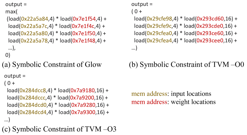
Figure 8: Mostly consistent symbolic constraints extracted from vastly different binaries.

Table 7: GitHub repo commits investigation results. We report the #Commits in the past two years, #Commits related to CPU code generation, the average LOC per CPU commit, and #CPU commits with substantial changes (over 100 LOC).

Compiler	#Commits	#CPU Commits	Avg. LOC	#Substantial
TVM	4,292	121	17	3
Glow	1,435	22	47	3
NNFusion	200	13	16	1

Second, we investigated commits related to CPU instruction generation in DL compilers’ GitHub repos over the past two years (April 2020 to April 2022). As in Table 7, while these compilers are frequently updated, most commits aim to increase support for alternative hardware and model formats, where CPU-related code has changed little. We manually reviewed all “substantial” commits, i.e., commits with more than 100 LOC changes, and confirmed that they do not change optimization strategies or binary code generation that may affect BTD. Besides, DL compilers heavily use parallel instruction extensions (e.g., SSE) to speed up model inference on CPUs. These extensions have been stable and unchanged over the long term. To answer RQ2, we again underline that BTD’s essential assumption is that symbolic constraints extracted from each DNN operator’s assembly function should be invariant across compilers and optimizations. Other features, such as function signatures, operator fusion, and optimization strategies, are independent of BTD’s core techniques and are also unlikely to be largely changed in the near future.

7.3 RQ3: Extensibility

Table 8: Categorize ONNX operators. #with Dims. denotes #operators with dimensions to be recovered, #with Opt. denotes #operators with compile-time optimizations, Workload denotes the amount of work required to cover new operators, and #Covered denotes #operators that currently supported.

Category	#OPs	#with Dims.	#with Opt.	Workload	#Covered
Element-wise Op	56	2	0	Low	2/2
Tensor Op	32	8	0	Low	6/8
Matrix Op	2	0	0	NA	NA
Pooling	9	9	0	Low	5/9
Heavyweight	11	11	11	High	7/11
Normalization	6	6	0	Low	2/6
Transpose	8	0	0	NA	NA
Random	6	0	0	NA	NA
Others	33	0	0	NA	NA
Total	163	36	11	NA	22/36*

• 22 of the 36 operators with dimensions that require specific patterns to recover are already covered in BTD. 4 of the remaining 8 operators can be covered with low effort, and the rest 4 (ConvInteger, MatMulInteger, QLinearConv, and QLinearMatMul) are rare in common models.

As stated in Sec. 7.1, BTD can cover all operators used in the CV models from ONNX Zoo. This section measures BTD’s extensibility through the lens of all DNN operators supported by ONNX Zoo (RQ3). Note that not all operators are for CV models, and not all operators have been used in DNN models; some of them are rarely used in common models. Overall, while most techniques (i.e., operator inference and symbolic execution) used in BTD are independent of operator types, patterns described in Sec. 4.3.3 are designed for each complex operator to recover their parameters/dimensions. Supporting a new operator may need new or existing patterns. Symbolic constraints are generally human readable, and we typically need several hours to design and validate a new pattern for operators without complex optimization, like BiasAdd and Pooling. Developing new patterns for complex operators like Conv may take days due to complex optimization strategies.

We classified all ONNX operators [9] to scope BTD’s applicability and the engineering effort required to extend BTD. Consider Table 8, where Low in workload column represents hours of effort, and High represents several days of work. While ONNX has 163 DNN operators [9], most of them do not have dimensions to be recovered. Besides, our patterns can be reused with minor modifications to support currently uncovered tensor operators, pooling operators, and normalization operators. For heavyweight calculation (Conv, MatMul/FC, GRU, RNN, LSTM, and their variants), we have already covered 7 out of 11 operators. Note that GRU, RNN, and LSTM can be covered because they are decomposed into sub-operators, including FC and element-wise operators, as explained in Sec. 7.1.7. Standard models rarely use the remaining operators, including ConvInteger, MatMulInteger, QLinearConv, and QLinearMatMul. BTD cannot handle these four operators for the time being, but we expect it will not be challenging to design patterns for these operators. Essentially, they are variants of Conv and MatMul operators. We leave support for these operators to our future work.

7.4 RQ4: Error Fixing

This section clarifies how BTD performs error fixing (RQ4). On one hand, with rules presented in Sec. 6, BTD can detect and automatically fix the errors exposed when decompiling the ResNet18 executable (compiled with TVM -O0). The recovered model specification, after fixing, are completely correct, as noted in Table 5. We detail the error fixing procedure as a case study over the ResNet18 executable in Appendix E.

On the other hand, when errors can not be fixed automatically (ResNet compiled with TVM -O3), users are required to read the symbolic constraints and fix errors manually. Generally, fixing an error requires users to be familiar with both standard operators used in DL models and x86 assembly language. Nevertheless, even partially recovered models may boost attacks like query-based model extraction [96, 79].

8 Discussion

Downstream Applications & Countermeasures. Previous model extraction attacks rely on repetitive queries or side channels to leak parts of DNNs. BTD, as a decompiler, reveals a new and practical attack surface to recover full DNNs when DNN executables are accessible. Appendix D will show that BTD can boost DNN attacks. In addition, legacy DNN executables can be inspected, hardened, and migrated to new platforms. To show the feasibility, we migrated decompiled x86 DNN executables onto GPUs. This step only requires to use different compiler options over our recovered DNN models.

DNNs may provide business advantages. Potential security concerns raised by BTD may be mitigated using obfuscation [54]; particularly, code obfuscation could likely impede DNN operator inference whereas data obfuscation may likely undermine our patterns over memory layouts.

Cross-Platform. As reviewed in Sec. 2, DL compiler can generate executables on various platforms. The core techniques of BTD are platform independent. We analyze the cross-platform extension of BTD from the following aspects. First, decompiling DNN executables on devices like hardware accelerators requires appropriate disassemblers. This demands vendor support and considerable engineering work. While certain GPU makers like Nvidia provides disassemblers [5], the architecture and ISA of such devices are only partially or not revealed, preventing migrating BTD to these devices. Intel recently released a dynamic instrumentation tool, GTPin [7], but it is immature and limited to Intel processor graphics. Without vendor support, it is extremely difficult, if not impossible, to implement disassemblers and dynamic instrumentors on our own for various devices.

Second, DL compilers produce distinct executables on GPUs and CPUs. For example, TVM creates a standalone DNN executable on CPU, but a runtime library, including detailed model information, and an OpenCL/CUDA executable on GPU. Glow has an immature support for OpenCL using JIT. In short, we see x86 CPU decompilation as more difficult because inputs are typically standalone executables.

9 Related Work

Software Reverse Engineering. Software decompilation has achieved primary success. Algorithms are proposed to improve decompiled C/C++ code, including refining type recovery [56, 87], variable recovery [19, 15], and control structure recovery [31, 33]. ML accelerates decompilation [34, 38, 52, 26]. Some decompilers are commercially available [41, 1, 2]. In addition, recent works have designed decompilers for Ethereum smart contracts [115, 36]. We focus on decompiling DNN executables by addressing domain challenges to convert DNN executables to high-level models. We envision that BTD will meet demands to comprehend, exploit, and harden real-world DNN executables.

Model Extraction. We have reviewed DL compilation techniques in Sec. 2. BTD enables a novel perspective to extract DNN models. As introduced in Sec. 3, current model extraction works mostly take “black-box” forms [79, 76, 94, 78], where adversaries can assemble a training dataset $(x,y)$ by continuously feeding inputs $x$ to a target model and collecting its prediction outputs $y$. The resulting training datasets can be used to train a local model. Side channels leaked during inference are also used for model extraction, including timing, cache, and power side channels [46, 104, 30, 105, 45, 116]. BTD is orthogonal to these side channel-based methods. As noted in Sec. 2, BTD can recover full model information whereas they conduct partial recovery. We also notice reverse engineering efforts targeting image processing software [66, 50, 13]. These works use static analysis and heuristics to map (assembly) image processing code (e.g., blurring) to high-level operators. They analyze image processing software (e.g., Photoshop), not DNN models.

10 Conclusion

We presented BTD, a decompiler for x86 DNN executables. BTD recovers full DNN models from executables, including operator types, network topology, dimensions, and parameters. Our evaluation reports promising results by successfully decompiling and further recompiling executables compiled from popular DNN models using different DL compilers.

Table 9: Average #instructions in logged and tainted traces.

Compiler	Operator	Logged Trace	Tainted Trace
Glow	Conv	12,494,354	104,377
	Convopt	5,025,031	21727
	FC	212,574	8,672
	MaxPool	1,288,057	NA
	AvgPool	6,804	NA
	LRN	1,726,037	NA
TVM -O0	Conv	368,697	41,571
	FC	3,090,359	110,643
	MaxPool	1,365,727	NA
	AvgPool	48,146	NA
	LRN	1,537,084	NA
	BiasAdd	294,656	NA
	Embedding	9,094	NA
TVM -O3	Conv	403,949	63,527
	FC	2,391,832	170,336
	MaxPool	1,374,641	NA
	AvgPool	193,490	NA
	LRN	1,577,524	NA
	BiasAdd	229,042	NA
	Embedding	20,640	NA

Table 10: Parameter/dimension inference. Lines 2–8 report each executable’s total #dimensions, correctly-inferred dimensions, and accuracy rate for dimension inference. Lines 9–15 report total #parameters and accuracy rate for parameter inference. Different versions of the same compiler produce the same results, therefore we merge their columns.

Model	Glow	TVM -O0	TVM -O3
	(2020, 2021, 2022)	(v0.7, v0.8, v0.9.dev)	(v0.7, v0.8, v0.9.dev)
ResNet18	65/65/100%	51/47/92.15%	78/78/100%
VGG16	54/54/100%	59/59/100%	52/52/100%
FastText	7/7/100%	7/7/100%	7/7/100%
Inception	235/235/100%	223/223/100%	222/222/100%
ShuffleNet	82/82/100%	71/71/100%	71/71/100%
MobileNet	124/124/100%	144/144/100%	125/125/100%
EfficientNet	133/133/100%	133/133/100%	132/132/100%
ResNet18	11,684,712/100%	11,703,912/99.37%	11,684,712/99.37%
VGG16	138,357,544/100%	138,357,544/100%	138,357,544/100%
FastText	2,500,101/100%	2,500,101/100%	2,500,101/100%
Inception	6,998,552/100%	6,998,552/100%	6,998,552/100%
ShuffleNet	2,270,514/100%	2,294,784/100%	2,270,514/100%
MobileNet	3,487,816/100%	3,487,816/100%	3,487,816/100%
EfficientNet	12,950,384/100%	12,966,032/100%	12,950,384/100%

Table 11: Recompilation. “NA” means that some errors in DNN models are not fixed, and thus the rebuilt models manifest inconsistent behavior.

Model	Glow	TVM -O0	TVM -O3
	(2020, 2021, 2022)	(v0.7, v0.8, v0.9.dev)	(v0.7, v0.8, v0.9.dev)
ResNet18	100%	100% (with fixing)	NA $\rightarrow$ 100%
VGG16	100%	100%	100%
FastText	100%	100%	100%
Inception	100%	100%	100%
ShuffleNet	100%	100%	100%
MobileNet	100%	100%	100%
EfficientNet	100%	100%	100%

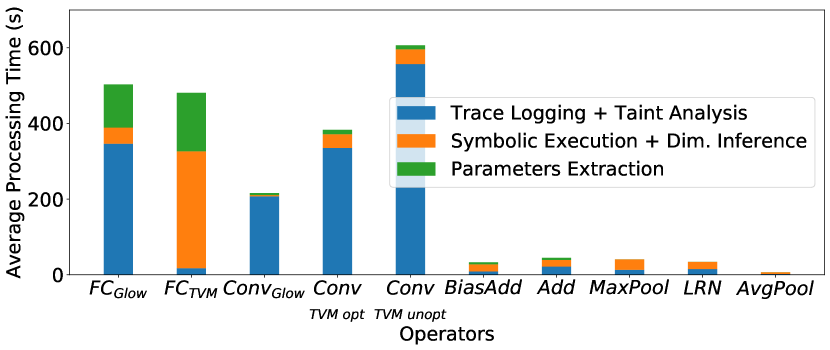
Figure 9: Processing time of parameter/dimension recovery.

Appendix A Processing Time

Recall Fig. 3(b) classifies DNN operators into four types. Fig. 9 reports the processing time of recovering parameters and dimensions over Type II, III, and IV operators encountered in our test cases. One DNN model can contain many instances of an operator, e.g., VGG16 has 13 instances of Conv. Fig. 9 reports the average cost of processing one instance.

Trace logging and tainting (Sec. 4.3.1) of Conv and FC operators can take several minutes; overall, taint analysis itself takes 48.6% of the processing time in blue bars. We further summarize the length of (tainted) traces in Table 9. In evaluation, we configure BTD to only conduct taint analysis for Conv and FC given that they generally emit much lengthy traces than other operators.

Table 9 illustrates that taint analysis is effective to largely reduce the trace size, which is also partially indicated by comparing blue bars and orange bars in Fig. 9. Thus, symbolic execution, a more heavyweight analysis, faces less instructions and is finished rapidly. Extracting parameters from memory (green bars) can also take several minutes. This is because popular CV models usually contain millions of parameters, and this step involves many I/O operations. Comparing $FC_{TVM}$ and $FC_{Glow}$, the former takes shorter time to log and taint traces. Nevertheless, we find that for $FC_{Glow}$, taint analysis taints only a succinct subtrace. Contrarily, a large portion of instructions are tainted for the $FC_{TVM}$ case, and therefore, its symbolic execution is still expensive.

Table 12: Configurations required to infer DNN operator parameters from corresponding assembly function arguments compiled by TVM.

Operator	Configuration
Conv	in, weights, out
Conv (fused)	in, weights, biases, out
Dense	in, weights, out
Dense (fused)	in, weights, biases, out
BiasAdd	in, biases, out
AveragePooling	in, out
MaxPooling	in, out
LRN	in, out
Sqrt	in, out
ReLU	in, out
Divide	in1, in2, out
Multiply	in1, in2, out
Negative	in, out
Flatten	in, out
Reshape	in, out
Transpose	in, out
Transform	in, out
Concatenate	in1, in2, out

Table 13: Configurations required to infer DNN operator parameters from corresponding assembly function arguments compiled by Glow.

Operator	Configuration
Conv	out, in, weights, biases
ConvDKKC8	out, in, weights, biases
Matmul	out, in, weights
MatmulAdd	out, in, weights, biases
MaxPooling	in, out
AveragePooling	in, out
ReLU	in/out
BatchAdd	out, in, biases
Transpose	in, out, dims
Reshape	in, out
Pad	in, out
Squeeze	in, out
AddReLU	in1/out, in2
ExtractTensor	in, out, offset
InsertTensor	in1/out, in2, offset
LocalResponseNormalization	out, in

Appendix B Assembly Function Prototypes for DNN Operators

As has clarified in the main paper, the calling convention of DNN executables have eased the task of localizing inputs and parameters for each DNN operator: we use Intel Pin [63] to hook callsites of assembly functions belonging to the DNN operators, and log the starting addresses of parameters and inputs during runtime.

With respect to different DNN operators, we pre-define configurations to describe their assembly function prototypes, particularly the meaning of each function parameter. Table 12 and Table 13 report the full configurations in BTD. Table 12 describes the assembly function prototypes in TVM-emitted executables. For instance, the configuration of Conv indicates that there are three arguments in its compiled assembly function, where the 1st argument is a pointer toward Conv inputs, the 2nd argument points to Conv parameters (i.e., weights), and the 3rd argument points to Conv outputs. In optimized code (TVM -O3), Conv operators are often fused with following BiasAdd operators which contribute “Bias”. As a result, the assembly function of Conv accepts two pointers toward the global memory regions of weights and biases, respectively. Similarly, Table 13 reports the assembly function prototypes in Glow-emitted executables. Note that some optimized Conv operators are renamed as ConvDKKC8 by Glow. AddReLU has two inputs, where one input (in₁) shares the memory region with the output.

Appendix C Parameters & Dimensions Recovery

BTD can recover dimensions and parameters of commonly-used DNN operators. We have demonstrated the comprehensiveness by showing that all DNN operators that exist in all CV models provided by ONNX Zoo [77] can be processed by BTD.

General Procedure. Due to the limited space, our main paper only details the recovery of parameters and dimensions for the Conv operator, which is also the most complex operator BTD needs to solve. As introduced in our main paper, we log execution trace using Intel Pin, simplify the trace with taint analysis, and then conduct symbolic execution to summarize invariant semantics in the form of symbolic constraints over inputs, parameters, and outputs. We then classify memory addresses collected over constraints into input addresses and parameter addresses. This way, we are able to gradually scope the memory layouts of inputs and parameters, thus inferring dimensions with patterns. Parameters are then dumped from memory to disk during runtime, and with the recovered dimensions, we are able to convert parameters (in data bytes dumped from memory) into well-formed parameters that can be directly processed by PyTorch.

In addition to solutions of Conv, the rest of this appendix section lists solutions of all other DNN operators that appear in our dataset. We emphasize that the General Procedure is indeed applicable to all DNN operators considered in this work. Given that said, patterns used to infer dimensions, as expected, need to be defined specifically for different operators. Also, Conv denotes the most complex DNN operator that requires the recovery of both parameters and dimensions. Many other operators only contain dimensions or parameters and only require simpler but more reliable patterns, as will be clarified below.

C.1 Fully-Connected (FC) Operator

FC operators are commonly-used to serve the last few operators of many popular DNN models. In general, neurons in a FC operator are fully connected to all activations in its previous operator. The activations of neurons in a FC operator can be typically computed with a matrix multiplication followed by a bias addition. Let the input $I$ of a FC operator be a matrix of size $(1,M)$, and the output $O$ be a matrix of size $(N,1)$. Hence, parameters $P$ of a FC operator can be represented as a $(M,N)$ matrix, and Bias $B$ is a matrix of $(N,1)$. The output can be calculated as $O=I\times P+Bias$.

Inferring Dimensions $M$ and $N$. For dimensions, we need to first recover the input memory size $M$ and the output memory size $N$. Given matrix multiplication $O=I\times P$ is performed in a FC operator, it is easy to see that each element $o$ in the output matrix of size $(N,1)$ is calculated using $M$ elements in the input and $M$ elements from the parameters $P$. Therefore, once we have performed symbolic execution to summarize the symbolic constraint over inputs, parameters and one output $o$, it is easy to infer $M$, by directly counting the number of multiplication that are found in the constraint. To infer $N$, we re-run Pin to log all memory writes, scope the size of the output region $M_{o}$, and divide $M_{o}$ by the size of an output element $o$. The size of $o$ is 4 bytes, denoting a 32-bit floating point number, on 64-bit x86 platforms.

C.2 Pooling Operator

A pooling operator downsamples the output of its prior operator. It is commonly used in dimension reduction to reduce the number of operations required for the following operators, but still retaining sufficient information from its previous operators. Despite that there are several different pooling schemes, e.g., max pooling (MaxPool), average pooling (AveragePool), and min pooling (MinPool), we infer the dimensions of pooling operators in a unified manner.

Patternss on Dimension Inference. In general, for a pooling operator, we need to recover its stride $S$ and the kernel size $K$. Similar with computations launched in a Conv operator, the pooling operator will iteratively extract a sub-matrix, namely kernel, for pooling. We clarify that kernel size $K$ is inferred in exactly the same way as how kernel size is inferred for Conv. To recover stride $S$, we first launch symbolic execution and generate the symbolic constraints for two consecutive output elements, namely $A$ and $B$. The offsets of input memory addresses shall indicate stride $S$. Specifically, we calculate $S$ through the following constraint:

$$S=\frac{addr_{1}-addr_{2}}{size}$$

where $addr_{1}$ denotes the smallest input address found in constraint $A$ and $addr_{2}$ denotes the smallest input address found in constraint $B$. $size$ denotes the size of one input element, which is 4 bytes in our research context.

C.3 Arithmetic Operators

In general, arithmetic operators in DNN models can be divided into two categories: parameterized operators and parameter-free operators. For parameter-free operators, such as Add, Sub, Div, Sqrt, which perform element-wise arithmetic operations over one (for Sqrt) or two inputs. Since the operations are element-wise, there is no dimension to be recovered.

For arithmetic operators with parameters, the memory starting addresses of parameters can be obtained from the assembly function inputs (see Table 12 and Table 13). Furthermore, we need to recover the size of parameters in order to dump parameters from memory. For example, DL compilers will use BiasAdd (or BatchedAdd) to implement the “add bias” operation in a Conv operator. To extract biases, we first need to know its size. However, the size of parameters cannot be inferred from the symbolic constraints, because the operation is element-wise, thus only one input element and one parameter will be involved in each symbolic constraint to compute an output element. Recall when analyzing Conv and FC, we use Pin to record all memory accesses toward parameters to gradually scope the memory region size of parameters. Similarly, here we conduct the same process to obtain the memory region size of biases.

C.4 Embedding Operator

Despite the popularity of DNN models in CV applications, natural language processing (NLP) models are also extensively adopted in real-life scenarios. Despite all common DNN operators that can be handled by BTD, Embedding is unique to NLP models. Embedding is frequently used to preprocess input text data by encoding text into embedding vectors. Embedding is essentially implemented as a hash table that maps semantically similar inputs to similar vectors in the latent embedding space. To recover an embedding operator, we need to infer the embedding dimension $D$ (the size of the embedding vector), and the number of embeddings $N$ (the size of the vocabulary or embedding table). For Glow-compiled executable, given that memcpy functions are used to implement Embedding, we can directly hook these memcpy functions and log its copied memory size, which equals to $D$. For TVM-compiled executable, to infer $D$, we use Pin to log all memory addresses that are accessed for memory read. The size of the longest and continuous memory chunk equals to $D$. To obtain $N$, we record the entire memory region of the embedding table used by Embedding, the size of which is denoted by $M$. Then, we compute $N$ as $\frac{M}{D}$.

C.5 Miscellaneous

Activation Functions. Typical DNN models include a large volume of non-linear activation functions like Sigmoid, Tanh, Softmax, and ReLU. To ease the presentation, we divide these activation functions into two categories: element-wise activations and tensor-wise activations. As aforementioned, element-wise activations like ReLU, Mish, and Tanh, will apply activation function one element each time. For cases of this category, there are no dimensions to be recovered. On the other hand, tensor-wise activations will apply activation functions to an $n$-dimensional input tensor, e.g., Softmax, Softmin, and LogSoftmax. For these cases, recovering the dimension $N$ of the input tensor is straightforward, given that for each symbolic constraint over inputs and one output element, the number of involved input elements equal to $N$.

Local Response Normalization (LRN). LRN usually follows a Conv operator, which applies normalization across channels. More specifically, the dimensions of output is the same as the dimension of input, and each output element is calculated using input elements from $n$ neighboring channels. While there is no parameter involved, we need to recover the number of neighboring channels $n$, as a configuration of LRN. As expected, given a LRN operator whose number of neighboring channels is $n$, there will be $n$ input elements involved in the symbolic constraint to compute one output element. Thus, we can infer $n$ by counting the number of input addresses found in the symbolic constraint.

Transpose, ExpandDims, Flatten, etc. These operators do not perform arithmetic operations. Instead, they change the dimensions, alter, or reshape the layout of inputs. We observed that such operators do not exist in the original model definition but are extra added by DL compilers to apply optimization strategies involving memory layout changes, as discussed in Sec. 7.1.6. Hence, while no parameters are involved in the computations, and such operators do not even exist in the original model, we ignore these operators during dimension recovery and model rebuilding.

Batch Normalization (BN). BN normalizes (e.g. scaling and shifting) operator inputs to enhance model learning quality and robustness. BN operators typically ship with parameters that were updated during training. The input and output dimensions are the same. It is worth noting that BN operators do not need to be handled specifically if the DL compiler optimizations are enabled: according to our observation, BN operators are typically fused with its prior operators (i.e., Conv) in the compiled executable, which changes the values of parameters in prior operators, but does not impede our solutions. In case that optimizations are disabled, BN operators are formed by simple arithmetic and utility operators. For example, when compiling with TVM -O0, the BN operator will be compiled as a sequence of basic arithmetic operations: [Add, Sqrt, Divide, Multiply, ExpandDims, Multiply, Negative, Multiply, Add, ExpandDims, Add.] ExpandDims can be ignored, as discussed above, and all of these arithmetic operators can be smoothly decompiled following the solution detailed in Sec. C.3.

InsertTensor, ExtractTensor, Concatenate, etc. Glow uses InsertTensor and ExtractTensor to do tensor level operations. For example, Glow may use InsertTensor to implement padding operations by inserting the input tensor into another wider tensor filled with zeros. Moreover, TVM uses Concatenate for similar operations. For these operators, we need to recover the attributes employed to manipulate tensors, such as offsets. According to our observation, such attributes are also passed to operators via arguments of assembly functions. Thus, we are able to get the attributes via instrumentation without using patterns.

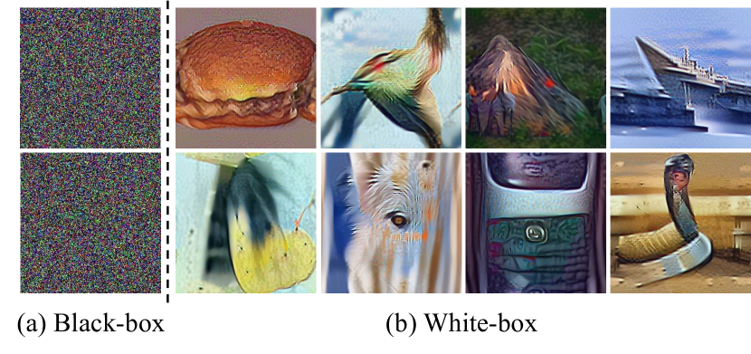
Figure 10: Images extracted from the ResNet18 executable (“black-box”) and from the decompiled ResNet18 model running on PyTorch (“White-box”).

Appendix D Boosting DNN Attacks

Many studies have been conducted on black-box attacks against DNN models [90, 79, 109, 106, 47]. However, these methods are usually time and resource intensive. While white-box attacks are more efficient, attackers may not have access to the white-box models [112, 57]. In our scenario, we assume that attackers with only DNN executables on hand as a black-box setting. In contrast, by decompiling DNN executables into high-level DNN specifications, BTD enables a white-box attack where attackers can inspect the internals of decompiled DNN models running on DL frameworks like TensorFlow or PyTorch. At this step, we present two case studies in which we 1) launch black-box attacks toward ResNet18 executable compiled by TVM -O3, 2) use BTD to decompile ResNet18 executable, and 3) launch white-box attacks toward the recovered ResNet18 running on PyTorch. We compare the attack effectiveness to illustrate the improvement of white-box settings over the black-box settings. We give the major setups and results below; for attack details, see Appendix G.

Adversarial Example Generation. Adversarial examples (AEs) are crafted inputs with the purpose of confusing a DNN [71, 68]. Typical black-box AE generation rely on a large number of time-consuming queries [79, 60]. To enhance AE generation on DNN executables, we first decompile the DNN executable of ResNet18 compiled with TVM -O3, and deploy the decompiled ResNet18 on PyTorch. We then employ white-box attack using the gradients acquired from the decompiled ResNet18 model. We employ the projected gradient descent (PGD) attack [65] for the white-box scenario and the state-of-the-art (SOTA) AE generation method for the black-box scenario [37]. Within 20 minutes, we can successfully generate 34,780 AEs using the white-box attack, compared to only 228 AEs using the black-box attack. The result is intuitive: white-box AE generation enabled by BTD can largely outperform the black-box attack.

Knowledge Stealing. Knowledge stealing, also known as knowledge transfer [42, 107], is the process by which knowledge is extracted from a victim DNN model. DeepInversion [107], the SOTA “data-free” knowledge stealing technique, requires no training data but only the victim model $m$. DeepInversion synthesizes images from $m$; it is shown that the synthesized images can be used to train another model with competitive accuracy [107]. It is easy to see that DeepInversion can steal intellectual property subsumed in well-trained DNN models in the form of synthesized images. Nevertheless, a DNN executable, denoting a black-box setting, can hardly enable knowledge stealing since it does not provide gradients. To enable knowledge stealing, we first use BTD to decompile the ResNet18 executable. We then launch the knowledge stealing process toward the decompiled ResNet18 (running on PyTorch). We use DeepInversion on both the ResNet18 executable and the decompiled model. For the black-box setting, we use a heuristic-based search strategy to replace standard gradient-based methods (details in Appendix G). As illustrated in Fig. 10, DeepInversion is capable of smoothly generating quality images from the decompiled ResNet18, indicating the success of knowledge stealing attack. In contrast, in the black-box scenario, only random noise is generated.

Appendix E Error Fixing Case Study

We introduced the error detection rules we used to automatically detect and fix errors in BTD’s output in Sec. 6. In this section, we provide a case study to show why some errors are fixable. Fig. 11 shows that BTD recovers the filter shape of a Conv as $[8.44,16,6,6]$ wrongly, because of the reshape optimization described in Case One in Sec. 7.1.6. Such an abnormal shape will be detected as an error by Rule 1 proposed in Sec. 6.

To fix this error, Rule 1 leverages input/output shapes from successor/predecessor operators to determine the input and output shape of the current Conv operator. As illustrated in Fig. 11, combining the input shape $[1,64,56,56]$, output shape $[1,128,28,28]$, and symbolic constraint, we are able to infer the input channel $I_{c}$ as $64$, and output channel $O_{c}$ as $128$. Assume the number of multiplications in constraint is $n$ ($576$ in this case study), we are also able to infer the kernel size $K$ as $\sqrt{\frac{n}{I_{c}}}$, i.e., $3$. Thus, the dimension of the Conv is automatically fixed as $[128,64,3,3]$.

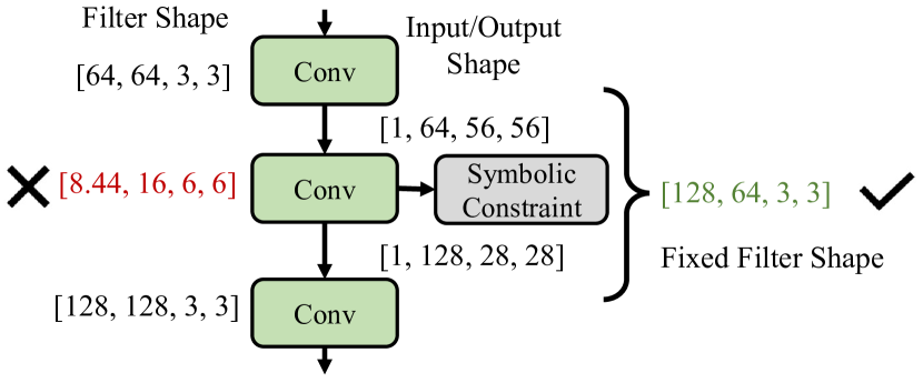
Figure 11: Error Fixing Case Study.

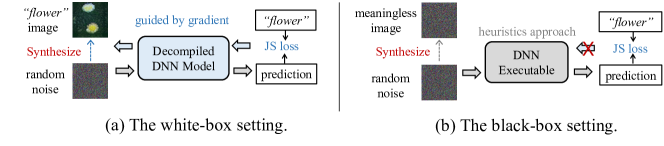
Figure 12: Overflow of data free knowledge distillation.

Appendix F Recovering Parameters From Optimized Memory Layouts

Our main paper has clarified that parameters of Conv can be dumped from memory with its starting address obtained from assembly function inputs together with the inferred dimensions. However, to take full advantage of SSE parallelism on x86 platforms, DL compilers may perform layout alteration optimization to change the standard memory layout of parameters. Overall, we find that Glow may change the memory layout from $[O_{C},I_{C},W,C]$ into $[O_{C}/A,I_{C},K,K,A]$ (as shown in Fig. 7). Similarly, TVM may change the layout into a $6$-dimensional tensor $[O_{C}/B,I_{C}/A,K,K,A,B]$.

Hence, inferring $A$ and $B$ becomes a pre-requisite to comprehend the optimized memory layouts. Given a summarized symbolic constraint over inputs, parameters, and one output element, we extract the memory offsets (w.r.t. the smallest memory address on the constraint) of all memory addresses belonging to weights, which will derive the following expression:

$$[$$

$$Y_{0}[ x_{0,0},\ x_{0,1},\ ...,\ x_{0,(W-1)},$$

$$x_{1,0},\ x_{1,1},\ ...,\ x_{1,(W-1)},$$

$$,\ ...,$$

$$x_{(A-1),0},\ x_{(A-1),1},\ ...,\ x_{(A-1),(W-1)}],$$

$$Y_{1}[ ...,\ ...,\ ...],$$

$$,...,$$

$$Y_{C\times H/A}[ x_{0,0},\ x_{0,1},\ ...,\ x_{0,(W-1)},$$

$$x_{1,0},\ x_{1,1},\ ...,\ x_{1,(W-1)},$$

$$,\ ...,$$

$$x_{(A-1),0},\ x_{(A-1),1},\ ...,\ x_{(A-1),(W-1)}]$$

$$]$$

where each $x_{i,j}$ is a memory offset of one weight element (i.e., the memory address of one small box in the optimized memory layout in Fig. 7). Here $Y$ is a notation to ease the representation, otherwise $x$ will be defined using 3 dimensions.

Furthermore, the optimized memory layout in Fig. 7 can indeed derive the following constraint

$$Y_{k}[x_{i,j}]=(i-1)\times B+j\times A\times B+k\times W\times A\times B$$

Hence, $A$ and $B$ can be inferred, by matching the above constraint with two elements in the extracted memory offsets, e.g., $Y_{0}[x_{0,1}]$ and $Y_{0}[x_{0,3}]$.

For example, let the offset list of weight memory addresses in a symbolic constraint be

$$[0,1024,2048,32,1056,2080,64,1088,2112,...]$$

, and the filter shape $[O_{C},I_{C},K,K]$ recovered in advance be $[256,128,3,3]$. From the 2nd offset in the list, we can infer that $A\times B=1024$. Similarly, from the 4th offset, we can infer that $B=32$. This way, $A$ and $B$ are recovered, and the layout configuration becomes $[O_{C}/32,I_{C}/32,K,K,32,32]=[256/32,128/32,3,3,32,32]$. Knowing the layout can enable smoothly loading all parameters out from memory and re-forming the original filter weights in Conv.

Appendix G Setup Details of Attacks Boosted by BTD

For the case study presented in Appendix D, the target of attacks is decided as the DNN executable of ResNet18 downloaded from ONNX Zoo [77] and compiled by TVM with full optimizations. The attacks are launched using a Nvidia RTX 2080 GPU.

Adversarial Examples Generation (AE). We launch the adversarial attack with seed images from ImageNet. We reuse the publicly available implementation [8] of Projected Gradient Descent (PGD) [65] over the decompiled ResNet18 model specifications. This denotes the white-box setting where we can fully access model gradients. Launching a white-box AE generation is standard and straightforward. The maximum perturbation is set to 0.3, the step size is set to 2/255 (where 255 is the maximal value of a pixel), and the total number of steps is set to 40. As reported in Appendix D, we successfully generate 34,780 AEs during a 20-minute experiment.

As for the black-box setting where attackers only have the executable file of ResNet18, we utilize the official release [4] of the state-of-the-art (SOTA) black-box AE generation attack [37]. We set the batch size as 50, the maximum perturbation as 0.3, a dimensionality of 2D frequency space as 14, and a sampling rate of 1,000 for the image samples. As noted in Appendix D, during a 20-minute experiment, we only successfully generate 228 AEs.

Knowledge Stealing. Knowledge stealing, also known as (data free) knowledge transfer, is a technique to extract knowledge (in terms of training data) in well-trained victim DNN to train a new “student” model. We employ the official PyTorch implementation [3] of DeepInversion [107] for the implementation. During distillation, the learning rate is set to 0.25, the regularization coefficient is set to 0.01, and the batch size is set to 84. As illustrated in Fig. 12, we employ Jensen-Shannon divergence as the loss function for back propagation in the white-box setting. However, in the black-box setting, we employ a heuristic-based search strategy to update the seed input, as back propagation is not possible.

As has illustrated in Fig. 10, for the white-box setting, it generates images with notably much higher quality compared to that of the black-box setting. This illustrates that heuristic-based approaches are hard to steal knowledge from the victim model, whereas BTD, by successfully decompiling the ResNet18 executable into high-level model descriptions, enables gradient-based methods that are much more powerful.

References

- [1] Hopper. https://www.hopperapp.com/, 2018.
- [2] JEB. https://www.pnfsoftware.com/, 2018.
- [3] Code for "Dreaming to Distill: Data-free Knowledge Transfer via DeepInversion" (CVPR 2020) . https://github.com/NVlabs/DeepInversion, 2021.
- [4] Code for ICML 2019 paper "Simple Black-box Adversarial Attacks" . https://github.com/cg563/simple-blackbox-attack, 2021.
- [5] Cuda binary utilities. https://docs.nvidia.com/cuda/cuda-binary-utilities/index.html, 2021.
- [6] Onnx. https://onnx.ai/, 2021.
- [7] Profiling tools interfaces for intel(r) processor graphics. https://github.com/intel/pti-gpu, 2021.
- [8] PyTorch implementation of adversarial attacks. https://github.com/Harry24k/adversarial-attacks-pytorch, 2021.
- [9] ONNX Operators . https://github.com/onnx/onnx/blob/main/docs/Operators.md, 2022.
- [10] PyTorch - Char-RNN. https://github.com/spro/practical-pytorch/blob/master/char-rnn-generation/char-rnn-generation.ipynb, 2022.
- [11] PyTorch - Sequence Models and LSTM, 2022. https://pytorch.org/tutorials/beginner/nlp/sequence_models_tutorial.html.
- [12] Andrew Adams, Karima Ma, Luke Anderson, Riyadh Baghdadi, Tzu-Mao Li, Michaël Gharbi, Benoit Steiner, Steven Johnson, Kayvon Fatahalian, Frédo Durand, et al. Learning to optimize halide with tree search and random programs. ACM TOG, 38(4):1–12, 2019.
- [13] Maaz Bin Safeer Ahmad, Jonathan Ragan-Kelley, Alvin Cheung, and Shoaib Kamil. Automatically translating image processing libraries to halide. ACM TOG, 38(6):1–13, 2019.
- [14] Amazon. Amazon SageMaker Neo uses Apache TVM for performance improvement on hardware target. https://aws.amazon.com/sagemaker/neo/, 2021.
- [15] Kapil Anand, Matthew Smithson, Khaled Elwazeer, Aparna Kotha, Jim Gruen, Nathan Giles, and Rajeev Barua. A compiler-level intermediate representation based binary analysis and rewriting system. In EuroSys, 2013.
- [16] Dennis Andriesse, Xi Chen, Victor Van Der Veen, Asia Slowinska, and Herbert Bos. An in-depth analysis of disassembly on full-scale x86/x64 binaries. In 25th USENIX Security 16, pages 583–600, 2016.
- [17] Riyadh Baghdadi, Jessica Ray, Malek Ben Romdhane, Emanuele Del Sozzo, Abdurrahman Akkas, Yunming Zhang, Patricia Suriana, Shoaib Kamil, and Saman Amarasinghe. Tiramisu: A polyhedral compiler for expressing fast and portable code. In CGO 2019, pages 193–205. IEEE, 2019.
- [18] Dzmitry Bahdanau, Kyunghyun Cho, and Yoshua Bengio. Neural machine translation by jointly learning to align and translate. arXiv preprint arXiv:1409.0473, 2014.
- [19] Gogul Balakrishnan and Thomas Reps. Wysinwyx: What you see is not what you execute. ACM Trans. Program. Lang. Syst., 32(6):23:1–23:84, August 2010.
- [20] Piotr Bojanowski, Edouard Grave, Armand Joulin, and Tomas Mikolov. Enriching word vectors with subword information. TACL, 5:135–146, 2017.
- [21] David Brumley, JongHyup Lee, Edward J. Schwartz, and Maverick Woo. Native x86 decompilation using semantics-preserving structural analysis and iterative control-flow structuring. In USENIX Security 13, pages 353–368, 2013.
- [22] Tianqi Chen, Thierry Moreau, Ziheng Jiang, Lianmin Zheng, Eddie Yan, Haichen Shen, Meghan Cowan, Leyuan Wang, Yuwei Hu, Luis Ceze, et al. TVM: An automated end-to-end optimizing compiler for deep learning. In 13th USENIX OSDI, pages 578–594, 2018.
- [23] Tianqi Chen, Lianmin Zheng, Eddie Yan, Ziheng Jiang, Thierry Moreau, Luis Ceze, Carlos Guestrin, and Arvind Krishnamurthy. Learning to optimize tensor programs. NeurIPS, 31:3389–3400, 2018.
- [24] Sharan Chetlur, Cliff Woolley, Philippe Vandermersch, Jonathan Cohen, John Tran, Bryan Catanzaro, and Evan Shelhamer. cuDNN: Efficient primitives for deep learning. arXiv preprint arXiv:1410.0759, 2014.
- [25] Cristina Cifuentes and K. John Gough. Decompilation of binary programs. Softw. Pract. Exper., 25(7):811–829, July 1995.
- [26] Yaniv David, Uri Alon, and Eran Yahav. Neural reverse engineering of stripped binaries using augmented control flow graphs. OOPSLA, 2020.
- [27] Jia Deng, Wei Dong, Richard Socher, Li-Jia Li, Kai Li, and Li Fei-Fei. ImageNet: A large-scale hierarchical image database. In CVPR, pages 248–255. IEEE, 2009.
- [28] S. H. Ding, B. M. Fung, and P. Charland. Asm2Vec: Boosting static representation robustness for binary clone search against code obfuscation and compiler optimization. In IEEE S&P, 2019.
- [29] Yue Duan, Xuezixiang Li, Jinghan Wang, and Heng Yin. DeepBinDiff: Learning program-wide code representations for binary diffing. In NDSS, 2020.
- [30] Vasisht Duddu, Debasis Samanta, D Vijay Rao, and Valentina E Balas. Stealing neural networks via timing side channels. arXiv preprint arXiv:1812.11720, 2018.
- [31] Khaled ElWazeer, Kapil Anand, Aparna Kotha, Matthew Smithson, and Rajeev Barua. Scalable variable and data type detection in a binary rewriter. In PLDI, 2013.
- [32] Bauman Erick, Lin Zhiqiang, and Hamlen Kevin W. Superset disassembly: Statically rewriting x86 binaries without heuristics. In NDSS, 2018.
- [33] Antonio Flores-Montoya and Eric Schulte. Datalog disassembly. In 29th USENIX Security, 2020.
- [34] Cheng Fu, Huili Chen, Haolan Liu, Xinyun Chen, Yuandong Tian, Farinaz Koushanfar, and Jishen Zhao. Coda: An end-to-end neural program decompiler. NeurIPS, 32:3708–3719, 2019.
- [35] Philip Gage. A new algorithm for data compression. C Users Journal, 12(2):23–38, 1994.
- [36] Neville Grech, Lexi Brent, Bernhard Scholz, and Yannis Smaragdakis. Gigahorse: thorough, declarative decompilation of smart contracts. In ICSE, 2019.
- [37] Chuan Guo, Jacob Gardner, Yurong You, Andrew Gordon Wilson, and Kilian Weinberger. Simple black-box adversarial attacks. In ICML. PMLR, 2019.
- [38] Hossein Hajipour, Mateusz Malinowski, and Mario Fritz. IReEn: Iterative reverse-engineering of black-box functions via neural program synthesis. arXiv preprint arXiv:2006.10720, 2020.
- [39] Kaiming He, Xiangyu Zhang, Shaoqing Ren, and Jian Sun. Deep residual learning for image recognition. In CVPR, pages 770–778, 2016.
- [40] Shawn Hershey, Sourish Chaudhuri, Daniel PW Ellis, Jort F Gemmeke, Aren Jansen, R Channing Moore, Manoj Plakal, Devin Platt, Rif A Saurous, Bryan Seybold, et al. Cnn architectures for large-scale audio classification. In ICASSP, pages 131–135. IEEE, 2017.
- [41] SA Hex-Rays. IDA Pro: a cross-platform multi-processor disassembler and debugger, 2014.
- [42] Geoffrey Hinton, Oriol Vinyals, and Jeff Dean. Distilling the knowledge in a neural network. arXiv preprint arXiv:1503.02531, 2015.
- [43] Sepp Hochreiter and Jürgen Schmidhuber. Long short-term memory. Neural computation, 1997.
- [44] Andrew G Howard, Menglong Zhu, Bo Chen, Dmitry Kalenichenko, Weijun Wang, Tobias Weyand, Marco Andreetto, and Hartwig Adam. Mobilenets: Efficient convolutional neural networks for mobile vision applications. arXiv preprint arXiv:1704.04861, 2017.
- [45] Xing Hu, Ling Liang, Shuangchen Li, Lei Deng, Pengfei Zuo, Yu Ji, Xinfeng Xie, Yufei Ding, Chang Liu, Timothy Sherwood, et al. Deepsniffer: A dnn model extraction framework based on learning architectural hints. In ASPLOS, pages 385–399, 2020.
- [46] Weizhe Hua, Zhiru Zhang, and G Edward Suh. Reverse engineering convolutional neural networks through side-channel information leaks. In DAC, pages 1–6. IEEE, 2018.
- [47] Zhichao Huang and Tong Zhang. Black-box adversarial attack with transferable model-based embedding. In ICLR, 2019.
- [48] Texas Instruments. The AM335x microprocessors support TVM. https://software-dl.ti.com/processor-sdk-linux/esd/docs/latest/linux/Foundational_Components/Machine_Learning/tvm.html, 2021.
- [49] Animesh Jain, Shoubhik Bhattacharya, Masahiro Masuda, Vin Sharma, and Yida Wang. Efficient execution of quantized deep learning models: A compiler approach. arXiv preprint arXiv:2006.10226, 2020.
- [50] Shoaib Kamil, Alvin Cheung, Shachar Itzhaky, and Armando Solar-Lezama. Verified lifting of stencil computations. In PLDI, New York, NY, USA, 2016.
- [51] Min Gyung Kang, Stephen McCamant, Pongsin Poosankam, and Dawn Song. DTA++: dynamic taint analysis with targeted control-flow propagation. In NDSS, 2011.
- [52] Deborah S Katz, Jason Ruchti, and Eric Schulte. Using recurrent neural networks for decompilation. In SANER, pages 346–356. IEEE, 2018.
- [53] Alex Krizhevsky, Ilya Sutskever, and Geoffrey E Hinton. Imagenet classification with deep convolutional neural networks. Advances in neural information processing systems, 25:1097–1105, 2012.
- [54] Per Larsen, Andrei Homescu, Stefan Brunthaler, and Michael Franz. SoK: Automated software diversity. In 2014 IEEE Symposium on Security and Privacy, pages 276–291. IEEE, 2014.
- [55] Chris Lattner and Vikram Adve. LLVM: A compilation framework for lifelong program analysis & transformation. In Proceedings of the International Symposium on Code Generation and Optimization: Feedback-directed and Runtime Optimization, CGO ’04, pages 75–, Washington, DC, USA, 2004. IEEE Computer Society.
- [56] JongHyup Lee, Thanassis Avgerinos, and David Brumley. TIE: Principled reverse engineering of types in binary programs. In NDSS, 2011.
- [57] Klas Leino and Matt Fredrikson. Stolen memories: Leveraging model memorization for calibrated white-box membership inference. In 29th USENIX Security, pages 1605–1622, 2020.
- [58] Mingzhen Li, Yi Liu, Xiaoyan Liu, Qingxiao Sun, Xin You, Hailong Yang, Zhongzhi Luan, Lin Gan, Guangwen Yang, and Depei Qian. The deep learning compiler: A comprehensive survey. TPDS, 2020.
- [59] Xuezixiang Li, Qu Yu, and Heng Yin. PalmTree: Learning an assembly language model for instruction embedding. In ACM CCS, 2021.
- [60] Yanpei Liu, Xinyun Chen, Chang Liu, and Dawn Song. Delving into transferable adversarial examples and black-box attacks. arXiv preprint, 2016.
- [61] Yizhi Liu, Yao Wang, Ruofei Yu, Mu Li, Vin Sharma, and Yida Wang. Optimizing CNN model inference on cpus. In USENIX ATC, pages 1025–1040, 2019.
- [62] Zhibo Liu and Shuai Wang. How far we have come: Testing decompilation correctness of C decompilers. In ISSTA, pages 475–487, 2020.
- [63] Chi-Keung Luk, Robert Cohn, Robert Muth, Harish Patil, Artur Klauser, Geoff Lowney, Steven Wallace, Vijay Janapa Reddi, and Kim Hazelwood. Pin: building customized program analysis tools with dynamic instrumentation. In PLDI, 2005.
- [64] Lingxiao Ma, Zhiqiang Xie, Zhi Yang, Jilong Xue, Youshan Miao, Wei Cui, Wenxiang Hu, Fan Yang, Lintao Zhang, and Lidong Zhou. Rammer: Enabling holistic deep learning compiler optimizations with rtasks. In 14th USENIX OSDI, pages 881–897, 2020.
- [65] Aleksander Madry, Aleksandar Makelov, Ludwig Schmidt, Dimitris Tsipras, and Adrian Vladu. Towards deep learning models resistant to adversarial attacks. In ICLR, 2018.
- [66] Charith Mendis, Jeffrey Bosboom, Kevin Wu, Shoaib Kamil, Jonathan Ragan-Kelley, Sylvain Paris, Qin Zhao, and Saman Amarasinghe. Helium: Lifting high-performance stencil kernels from stripped x86 binaries to halide dsl code. In PLDI, pages 391–402, New York, NY, USA, 2015. ACM.
- [67] Microsoft. Microsoft Linear Algebra Subprograms. https://github.com/microsoft/onnxruntime/tree/master/onnxruntime/core/mlas, 2021.
- [68] Seyed-Mohsen Moosavi-Dezfooli, Alhussein Fawzi, Omar Fawzi, and Pascal Frossard. Universal adversarial perturbations. In CVPR, pages 1765–1773, 2017.
- [69] Timothy Prickett Morgan. INSIDE FACEBOOK’S FUTURE RACK AND MICROSERVER IRON. https://www.nextplatform.com/2020/05/14/inside-facebooks-future-rack-and-microserver-iron/, 2020.
- [70] Ravi Teja Mullapudi, Andrew Adams, Dillon Sharlet, Jonathan Ragan-Kelley, and Kayvon Fatahalian. Automatically scheduling halide image processing pipelines. ACM TOG, 35(4):1–11, 2016.
- [71] Anh Nguyen, Jason Yosinski, and Jeff Clune. Deep neural networks are easily fooled: High confidence predictions for unrecognizable images. In CVPR, 2015.
- [72] Nvidia. CUDA. https://developer.nvidia.com/cuda-toolkit, 2021.
- [73] Nvidia. NVVM IR. https://docs.nvidia.com/cuda/nvvm-ir-spec/index.html, 2021.
- [74] NXP. NXP uses Glow to optimize models for low-power NXP MCUs. https://www.nxp.com/company/blog/glow-compiler-optimizes-neural-networks-for-low-power-nxp-mcus:BL-OPTIMIZES-NEURAL-NETWORKS, 2020.
- [75] OctoML. OctoML leverages TVM to optimize and deploy models. https://octoml.ai/features/maximize-performance/, 2021.
- [76] Seong Joon Oh, Bernt Schiele, and Mario Fritz. Towards reverse-engineering black-box neural networks. In Explainable AI: Interpreting, Explaining and Visualizing Deep Learning, pages 121–144. Springer, 2019.
- [77] ONNX. ONNX Zoo. https://github.com/onnx/models, 2021.
- [78] Tribhuvanesh Orekondy, Bernt Schiele, and Mario Fritz. Knockoff nets: Stealing functionality of black-box models. In CVPR, pages 4954–4963, 2019.
- [79] Nicolas Papernot, Patrick McDaniel, Ian Goodfellow, Somesh Jha, Z Berkay Celik, and Ananthram Swami. Practical black-box attacks against machine learning. In ACM Asia CCS, pages 506–519, 2017.
- [80] Adam Paszke, Sam Gross, Francisco Massa, Adam Lerer, James Bradbury, Gregory Chanan, Trevor Killeen, Zeming Lin, Natalia Gimelshein, Luca Antiga, et al. Pytorch: An imperative style, high-performance deep learning library. In NeurIPS, 2019.
- [81] Kexin Pei, Zhou Xuan, Junfeng Yang, Suman Jana, and Baishakhi Ray. TREX: Learning execution semantics from micro-traces for binary similarity. arXiv, 2021.
- [82] Huy Phan, Philipp Koch, Fabrice Katzberg, Marco Maass, Radoslaw Mazur, and Alfred Mertins. Audio scene classification with deep recurrent neural networks. Proc. Interspeech 2017, 2017.
- [83] Qualcomm. Qualcomm contributes Hexagon DSP improvements to the Apache TVM community. https://developer.qualcomm.com/blog/tvm-open-source-compiler-now-includes-initial-support-qualcomm-hexagon-dsp, 2020.
- [84] Jonathan Ragan-Kelley, Connelly Barnes, Andrew Adams, Sylvain Paris, Frédo Durand, and Saman Amarasinghe. Halide: a language and compiler for optimizing parallelism, locality, and recomputation in image processing pipelines. Acm Sigplan Notices, 2013.
- [85] Nadav Rotem, Jordan Fix, Saleem Abdulrasool, Garret Catron, Summer Deng, Roman Dzhabarov, Nick Gibson, James Hegeman, Meghan Lele, Roman Levenstein, et al. Glow: Graph lowering compiler techniques for neural networks. arXiv preprint, 2018.
- [86] Edward J Schwartz, Thanassis Avgerinos, and David Brumley. All you ever wanted to know about dynamic taint analysis and forward symbolic execution (but might have been afraid to ask). In IEEE SP, 2010.
- [87] Edward J. Schwartz, Cory F. Cohen, Michael Duggan, Jeffrey Gennari, Jeffrey S. Havrilla, and Charles Hines. Using logic programming to recover c++ classes and methods from compiled executables. In CCS, 2018.
- [88] Rico Sennrich, Barry Haddow, and Alexandra Birch. Neural machine translation of rare words with subword units. In ACL, pages 1715–1725, Berlin, Germany, August 2016. Association for Computational Linguistics.
- [89] Karen Simonyan and Andrew Zisserman. Very deep convolutional networks for large-scale image recognition. arXiv preprint arXiv:1409.1556, 2014.
- [90] Fnu Suya, Jianfeng Chi, David Evans, and Yuan Tian. Hybrid batch attacks: Finding black-box adversarial examples with limited queries. In 29th USENIX Security, pages 1327–1344, 2020.
- [91] Christian Szegedy, Wei Liu, Yangqing Jia, Pierre Sermanet, Scott Reed, Dragomir Anguelov, Dumitru Erhan, Vincent Vanhoucke, and Andrew Rabinovich. Going deeper with convolutions. In CVPR, 2015.
- [92] Christian Szegedy, Vincent Vanhoucke, Sergey Ioffe, Jon Shlens, and Zbigniew Wojna. Rethinking the inception architecture for computer vision. In CVPR, pages 2818–2826, 2016.
- [93] Mingxing Tan and Quoc Le. Efficientnet: Rethinking model scaling for convolutional neural networks. In ICML, pages 6105–6114. PMLR, 2019.
- [94] Daniel Teitelman, Itay Naeh, and Shie Mannor. Stealing black-box functionality using the deep neural tree architecture. arXiv preprint arXiv:2002.09864, 2020.
- [95] TensorFlow. XLA: Optimizing Compiler for TensorFlow. https://www.tensorflow.org/xla, 2022.
- [96] Florian Tramèr, Fan Zhang, Ari Juels, Michael K Reiter, and Thomas Ristenpart. Stealing machine learning models via prediction apis. In 25th USENIX Security, pages 601–618, 2016.
- [97] Nicolas Vasilache, Oleksandr Zinenko, Theodoros Theodoridis, Priya Goyal, Zachary DeVito, William S Moses, Sven Verdoolaege, Andrew Adams, and Albert Cohen. Tensor comprehensions: Framework-agnostic high-performance machine learning abstractions. arXiv preprint arXiv:1802.04730, 2018.
- [98] Ruoyu Wang, Yan Shoshitaishvili, Antonio Bianchi, Aravind Machiry, John Grosen, Paul Grosen, Christopher Kruegel, and Giovanni Vigna. Ramblr: Making reassembly great again. In NDSS, 2017.
- [99] Shuai Wang, Pei Wang, and Dinghao Wu. Reassembleable disassembling. In USENIX Security, 2015.
- [100] Shuai Wang and Dinghao Wu. In-memory fuzzing for binary code similarity analysis. In ASE, 2017.
- [101] Sally Ward-Foxton. Google and Nvidia Tie in MLPerf; Graphcore and Habana Debut. https://www.eetimes.com/google-and-nvidia-tie-in-mlperf-graphcore-and-habana-debut/#, 2021.
- [102] David Williams-King, Hidenori Kobayashi, Kent Williams-King, Graham Patterson, Frank Spano, Yu Jian Wu, Junfeng Yang, and Vasileios P Kemerlis. Egalito: Layout-agnostic binary recompilation. In ASPLOS, pages 133–147, 2020.
- [103] Ruoyu Wu, Taegyu Kim, Dave Jing Tian, Antonio Bianchi, and Dongyan Xu. Dnd: A cross-architecture deep neural network decompiler. In 31st USENIX Security, pages 2135–2152, 2022.
- [104] Yun Xiang, Zhuangzhi Chen, Zuohui Chen, Zebin Fang, Haiyang Hao, Jinyin Chen, Yi Liu, Zhefu Wu, Qi Xuan, and Xiaoniu Yang. Open dnn box by power side-channel attack. IEEE Transactions on Circuits and Systems II: Express Briefs, 2020.
- [105] Mengjia Yan, Christopher W Fletcher, and Josep Torrellas. Cache telepathy: Leveraging shared resource attacks to learn DNN architectures. In 29th USENIX Security, pages 2003–2020, 2020.
- [106] Jiancheng Yang, Yangzhou Jiang, Xiaoyang Huang, Bingbing Ni, and Chenglong Zhao. Learning black-box attackers with transferable priors and query feedback. NeuIPS, 33, 2020.
- [107] Hongxu Yin, Pavlo Molchanov, Jose M Alvarez, Zhizhong Li, Arun Mallya, Derek Hoiem, Niraj K Jha, and Jan Kautz. Dreaming to distill: Data-free knowledge transfer via deepinversion. In CVPR, 2020.
- [108] Zeping Yu, Rui Cao, Qiyi Tang, Sen Nie, Junzhou Huang, and Shi Wu. Order matters: Semantic-aware neural networks for binary code similarity detection. AAAI, 2020.
- [109] Jianhe Yuan and Zhihai He. Consistency-sensitivity guided ensemble black-box adversarial attacks in low-dimensional spaces. In ICCV, 2021.
- [110] Tomofumi Yuki, Gautam Gupta, DaeGon Kim, Tanveer Pathan, and Sanjay Rajopadhye. Alphaz: A system for design space exploration in the polyhedral model. In LCPC, pages 17–31. Springer, 2012.
- [111] Xiangyu Zhang, Xinyu Zhou, Mengxiao Lin, and Jian Sun. Shufflenet: An extremely efficient convolutional neural network for mobile devices. In CVPR, 2018.
- [112] Yinghua Zhang, Yangqiu Song, Jian Liang, Kun Bai, and Qiang Yang. Two sides of the same coin: White-box and black-box attacks for transfer learning. In KDD, pages 2989–2997, 2020.
- [113] Lianmin Zheng, Chengfan Jia, Minmin Sun, Zhao Wu, Cody Hao Yu, Ameer Haj-Ali, Yida Wang, Jun Yang, Danyang Zhuo, Koushik Sen, et al. Ansor: Generating high-performance tensor programs for deep learning. In 14th USENIX OSDI, pages 863–879, 2020.
- [114] Size Zheng, Yun Liang, Shuo Wang, Renze Chen, and Kaiwen Sheng. Flextensor: An automatic schedule exploration and optimization framework for tensor computation on heterogeneous system. In ASPLOS, 2020.
- [115] Yi Zhou, Deepak Kumar, Surya Bakshi, Joshua Mason, Andrew Miller, and Michael Bailey. Erays: reverse engineering ethereum’s opaque smart contracts. In 27th USENIX Security, pages 1371–1385, 2018.
- [116] Yuankun Zhu, Yueqiang Cheng, Husheng Zhou, and Yantao Lu. Hermes attack: Steal DNN models with lossless inference accuracy. In USENIX Security, 2021.