Dual-former: Hybrid Self-attention Transformer for Efficient Image Restoration

Abstract

Recently, image restoration transformers have achieved comparable performance with previous state-of-the-art CNNs. However, how to efficiently leverage such architectures remains an open problem. In this work, we present Dual-former whose critical insight is to combine the powerful global modeling ability of self-attention modules and the local modeling ability of convolutions in an overall architecture. With convolution-based Local Feature Extraction modules equipped in the encoder and the decoder, we only adopt a novel Hybrid Transformer Block in the latent layer to model the long-distance dependence in spatial dimensions and handle the uneven distribution between channels. Such a design eliminates the substantial computational complexity in previous image restoration transformers and achieves superior performance on multiple image restoration tasks. Experiments demonstrate that Dual-former achieves a 1.91dB gain over the state-of-the-art MAXIM method on the Indoor dataset for single image dehazing while consuming only 4.2% GFLOPs as MAXIM. For single image deraining, it exceeds the SOTA method by 0.1dB PSNR on the average results of five datasets with only 21.5% GFLOPs. Dual-former also substantially surpasses the latest desnowing method on various datasets, with fewer parameters.

I Introduction

Recently, non-trivial progress has been made in image restoration via data-driven CNNs methods (image dehazing [39], desnowing [8], deraining [66],image denoising [4], image debluring [27] and underwater enhancement [17]). The local inductive bias and translation invariance of the convolution operation bestow CNNs the advantages of local details modeling. However, CNN-based designs lack global modeling ability. To alleviate this problem, previous methods adopt gradual down-sampling to obtain a larger receptive field and enhance information interaction [66]. Nevertheless, the recovery performance of CNNs is still limited due to the lack of global modeling.

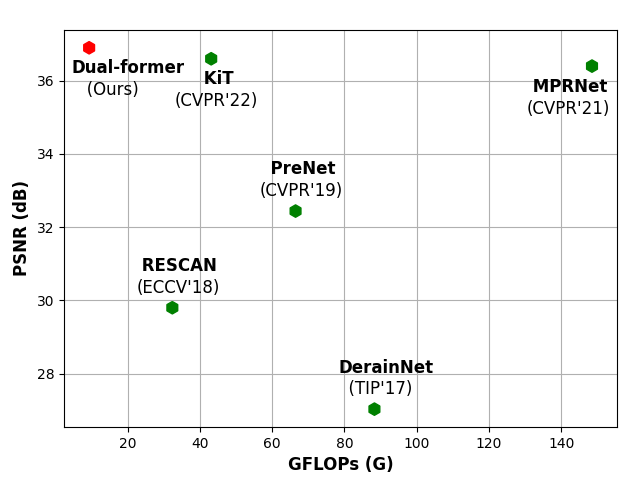
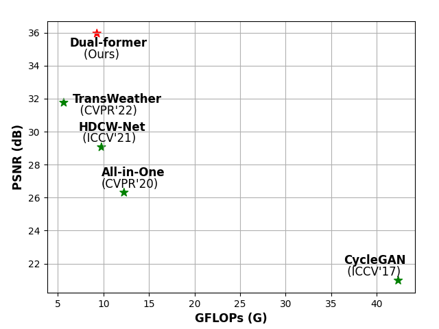
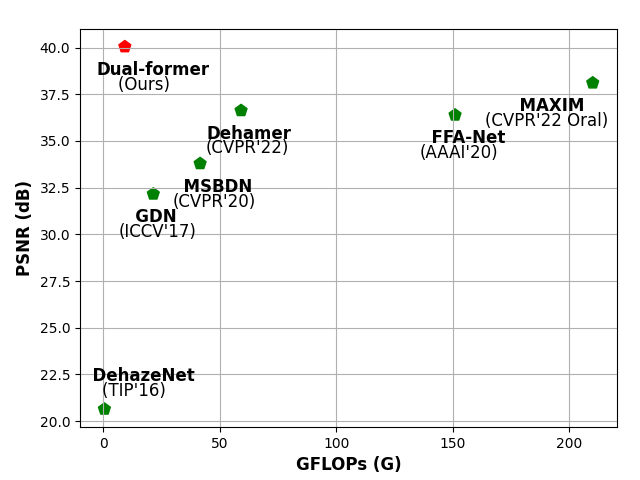
Figure 1: Top row: Image Restoration Architecture. (a) MPRNet [66] designs the multi-stage image restoration backbone, which progressive recovers the degradation image based on CNNs architecture. (b) KiT [28] consists of the k-NN Transformer Block, which utilizes the k-nearest patches obtained by the local-sensitive hashing. (c) Our Dual-former adopts the convolution-based block in encoder-decoder part and embeds the Hybrid Transformer Block into the latent layer to reduce computational complexity. Bottom row: Trade-off between PSNR performance v.s. the number of parameters on Rain100L [62], CSD [8] and Indoor [31] datasets. Dual-former achieves the best results on various datasets and still costs much less computation complexity than others.

Inspired by the natural language processing (NLP) [57], vision transformer [13] was proposed in the high-level tasks and aroused many wonderful works such as CvT [61], Levit [18], Mobile-former [9], MPViT [30]. Vision transformer exploits self-attention to model long-distance dependence, and has shown great potential in low-level vision tasks.

Nevertheless, there is a challenge for ViTs in high-resolution image restoration due to the quadratic relationship between self-attention computation and image size. To promote the performance and computation trade-off, lots of ViTs-based methods seek careful design to reduce computational burden. Uformer [59] utilized the window self-attention mechanism combined with the U-shape architecture to limit the amount of computation inside the window. Restormer [65] exploited channel-wise self-attention to reduce the computational complexity from square to linear. KiT [28] utilized locality-sensitive hashing, aggregating similar adjacent blocks to improve performance and also restrict computational burden. MAXIM [55] presented MLP-based modules: the multi-axis block and the cross-gating block, to perform global and local feature interaction with linear complexity. However, the above methods still have high computational complexities ($\mathbf{89.46G}$ for Uformer, $\mathbf{140.92G}$ for Restormer, $\mathbf{43.08G}$ for KiT and $\mathbf{216.0G}$ for MAXIM in terms of GFLOPs computed in 256$\times$256 resolution). Thus, it is important to design an effective ViT-based image restoration architecture with lower computational complexity.

Specifically, previous works such as Restormer [65] and KiT [28] used ViT-based modules in the overall framework unsuited for high-resolution features to reduce computational complexity compared with efficient CNNs. While the CNNs-based architecture easily encounters performance bottlenecks. As shown in Fig.1(a-b), MPRNet [66] based on CNNs still have performance limitation though it has cost substantial computational complexity. Conversely, KiT [28] operates self-attention to model global information and boost the network’s performance, while it needs an amount of computational complexity despite reducing computation by locality-sensitive hashing.

According to the study of feature representation [48], transformer-based frameworks such as ViT [13] primarily pays attention to global information in higher layers and it is hard to perform the local modeling in shallower stages. In order to combine the merits of CNNs and ViTs, we believe that it’s a good paradigm to use convolution-based modules for efficient local modeling while applying self-attention only in the latent layer for global modeling. To this end, we present the Dual-former, which achieves state-of-the-art performance in image restoration tasks with pretty low model complexity (only $\mathbf{9.28G}$ GFLOPs computed in 256×256 resolution). To elevate the efficiency of our framework, (i). we employ the simple yet effective conv-based $\mathbf{L}$ocal $\mathbf{F}$eature $\mathbf{E}$xtraction (LFE) module in the encoder-decoder part, which captures the local information cheaply in high-dimension space. (ii). We only embed the $\mathbf{H}$ybrid $\mathbf{T}$ransformer $\mathbf{B}$lock (HTB) into the latent layer. Compared with previous SOTA methods, this design significantly reduces the computational complexity.

For the Hybrid Transformer Block in the latent layer, we believe long-distance dependence modeling is necessary for image restoration at the spatial level. In addition, the uneven distributions for channel dimensions motivate us that performing sufficient channel global modeling is crucial for image restoration. Thus, we adopt the self-attention mechanism to obtain self-information from both channel and spatial dimensions. Considering the conflict of information from different dimensional perspectives, we propose an $\mathbf{A}$daptive $\mathbf{C}$ontrol $\mathbf{M}$odule (ACM) to fuse the information before implementing a Multi-Branch Feed-forward Network (MBFFN). Parallel to the Hybrid Transformer Block, we leverage our local feature extraction module to augment local information, aiming to enhance the overall representation power in the deepest layer.

Our contributions can be summarized as follows:

• Dual-former combines the merits of CNNs and ViTs via embedding them into different stages to facilitate the trade-off of efficiency and performance.

• A Local Feature Extraction module (LFE) is proposed to perform local modeling cheaply in high-dimension space via depth-wise convolution and channel attention, which aggregates local information for image restoration.

• We present the Hybrid Transformer Block (HTB), which adaptively controls the information from the hybrid self-attention of the channel and spatial dimensions simultaneously while cooperating with a local convolution block to improve model representation ability in the latent layer.

II Related Works

II-A Image Restoration

Image restoration is a typical low-level task that aims to restore clean images from degraded images. In recent years, deep learning methods based on convolutional neural networks (CNNs) has widely spread in the field of computer vision, especially in image restoration task, including dehazing [39, 64], deraining [66, 24], desnowing [8, 6], denoising [46, 23], debluring [10, 29] and low light enhancement [54, 26]. UNet [50] as a classic encoder-decoder backbone has been utilized in image restoration field, more advanced approaches followed this multi-scale design to process the degraded image version [1, 27, 25]. And inspired by other tasks, attention operation is often introduced to image restoration to make up for the lack of interactive information in a certain dimension [33, 11], such as channel dimension [22] or spatial dimension [69]. With the development of vision transformers, the superiority of global modeling in vision transformers has been migrated to image restoration such as window-based self attention [37], self-attention from channel interaction [65], and multi-scale Swin-transformer for image dehazing [3]. To learn more image restoration methods, NTIRE challenge reports [36] can be referred.

II-B Vision Transformers

With the efforts of researchers in the visual community, the transformer mechanism has been successfully applied to the field of computer vision [13] (ViT), which competes with the CNNs that have dominated for many years. Numerous excellent transformer backbone has been proposed based on it [58, 43, 9]. However, the quadratic computational complexity of the image size is a limitation for ViTs’ progress. PVT [58] embedded the transformer block into the pyramid structure, which can gradually reduce the feature size and increase the receptive field to benefit for dense prediction tasks. Swin Transformer [43] deliberated drawbacks of ViT and performed self-attention between tokes inside the windows, which kept the linear computation overhead. In addition, it also employed window shift operation to improve communication of window bridging. Many extraordinary architectures like these exemplary methods could be read carefully in  [42, 45].

In low-level vision tasks, more and more transformer-based architectures are introduced. Uformer [59] was based on Swin Transformer to form a U-shaped architecture for image restoration and shows magnificent performance. KiT [28] grouped k-nearest neighbor patches with locality-sensitive hashing (LSH), which outperformed the state-of-the-art approaches in image deraining.

Although ViTs have achieved impressive results in low-level vision tasks. However, since the above manners consist of single-type transformer-based blocks in general, its enormous computational complexity makes it difficult for the above models to accomplish a performance-computation trade-off. In this paper, we propose a Dual-former that exploits CNNs-based local feature extraction in the encoder and decoder parts. The self-attention operation only performs global modeling capability in the latent layer, which attracts SOTA performance in multiple tasks and has less computational complexity than previous methods.

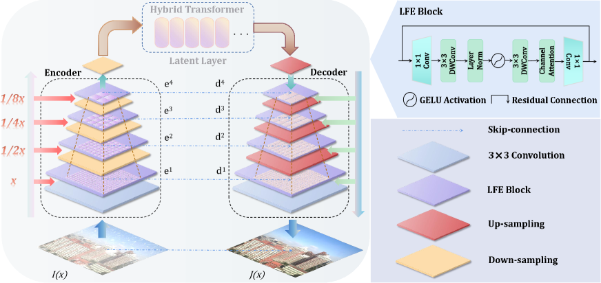
Figure 2: The left part is the proposed Dual-former framework. For the encoder-decoder, it consists of CNNs-based Local Feature Extraction (LFE) module. We devise the Hybrid Transformer Block (HTB) and embed it into the latent layer of the network. The upper right corner is the specific composition of our LFE block.

III Our Method

III-A Overall Architecture of Dual-former

The overall architecture of Dual-former is shown in Fig.2. Dual-former employs the CNNs-based encoder and decoder. The Hybrid Transformer block is only embedded in the latent layer to obtain the trade-off between performance and computational complexity. Given an input image $I(x)\in\mathbb{R}^{H\times W\times 3}$, we first utilize a 3$\times$3 convolution to project the image into feature. Then we adopt the proposed Local Feature Extraction (LFE) block to capture the local information, and use a 3$\times$3 convolution aiming to reduce the image’s resolution while expanding channel dimensions. Such action enriches the local receptive field in each encoder stage, which plays a crucial role in image restoration. The encoder can be formulated as follows:

$$X_{0}^{e}=\operatorname{LFE}(\operatorname{\varphi_{3}}(I(x))),$$ (1)

$$X_{i+1}^{e}=\operatorname{LFE}(X_{{i}}^{e}\in\mathbb{R}^{\frac{H}{2^{i}}\times\frac{W}{2^{i}}\times C_{i}}\downarrow),$$ (2)

where $X_{i+1}^{e}\in\mathbb{R}^{\frac{H}{2^{i+1}}\times\frac{W}{2^{i+1}}\times C_{i+1}}$ is the ($i$+1)-th feature of encoder, H, W, and C respectively denote the height, width and channel number of input image $I(x)$. $X$ is the feature of the input image. $\varphi_{3}$ and $\operatorname{LFE}$ are the 3$\times$3 convolution and LFE module. $\downarrow$ is the down-sampling operation. $i,i$+1 and $e$ represent the $i$-th and ($i$+1)-th stage of encoder. We set the i to 0, 1, 2 and 3 for each layer in this paper.

Unlike the previous ViT-based image restoration architectures that utilize the Transformer block in the entire network [37, 28, 59], we only use the self-attention mechanism in the latent layer. Due to its progressively extensive local receptive field, global self-attention could leverage local information well to perform global modeling. In Hybrid Transformer Block (HTB), we introduce self-attention from different dimension perspectives, where we perform spatial global modeling while paying attention to the channel self-information. In addition, we offer an Adaptive Control Module (ACM) to fusion the channel-spatial self-information. The Multi-branch Feed Forward Network is proposed to further improve the capacity of local inductive bias compared with previous feed-forward designs. In the latent layer, we can express it as the following formulas:

$$X_{4}^{l}=\operatorname{HTB}(X_{4}^{e}\in\mathbb{R}^{\frac{H}{16}\times\frac{W}{16}\times C_{l}}),$$ (3)

where the $l$ denotes the latent layer and $C_{l}$ is set to 384 in our paper. For the decoder part, we continue to compose the configuration of each stage with LFE module and gradually up-sample to the original resolution. Corresponding to each encoder stage, we add a skip connection to the decoder to avoid information loss. The decoder part can be defined by:

$$X_{i-1}^{d}=\operatorname{LFE}(X_{{i}}^{d}\in\mathbb{R}^{\frac{H}{2^{i}}\times\frac{W}{2^{i}}\times C_{i}}\uparrow+X^{e}_{i-1}),$$ (4)

$$J(x)=\operatorname{\varphi_{3}}(X_{0}^{d}+I(x)),$$ (5)

where $X_{4}^{d}=X_{4}^{l}$, ${X_{i-1}^{d}}\in\mathbb{R}^{\frac{H}{2^{i-1}}\times\frac{W}{2^{i-1}}\times C_{i-1}}$, the $d$ represents the decoder part of network. $J(x)$ is the clean image restored from degraded version. $\uparrow$ is the up-sampling operation. $+$ denotes skip connection that we utilize between each encoder and decoder [65]. We set the i to 4, 3, 2 and 1 for each decoder.

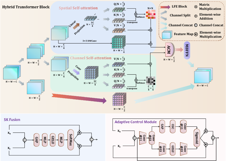
Figure 3: The upper part is our Hybrid Transformer Block (HTB). It consists of a mixture of spatial self-attention and channel self-attention mechanisms, as well as LFE modules. The lower left corner is the operation of SK fusion [53]. The lower right corner is the Adaptive Control Module (ACM) we designed, which strengthens the fusion of spatial interaction information and channel interaction information.

III-B Local Feature Extraction Block

For image restoration, local feature modeling determines the details of the restored image [65]. Convolution performs the merit of local modeling because of local inductive bias. Compared with the vanilla self-attention operation [13], the computation of convolution is not sensitive to the resolution of feature maps due to its $O(n)$ complexity. As shown in Fig.2, we present the Local Feature Extraction block (LFE) in the encoder and decoder to obtain rich feature information while saving computational complexity. Specifically, we believe high dimension space is crucial for the feature to perform local information modeling. Different from the  [65, 21], we first adopt a 1$\times$1 convolution to expand the number of dimensions. Then to achieve the trade-off between performance and computation complexity, we use two 3$\times$3 depth-wise convolutions to capture local information instead of 3$\times$3 convolutions. Besides, we adopt a Layer Normalization operation and a GELU activation function between them to consolidate training and optimize the nonlinear ability of the network. Channel attention has been proven effective for image restoration [4]. However, its performance is limited in shallow layers due to the number of channels. To tackle this issue, we add channel attention [22] after convolutions to further improve channel information interaction in high-dimension space. Finally, we utilize a residual connection [21] to enhance the proposed block’s robustness.

III-C Hybrid Transformer Block

In the latent layer, we design a Hybrid Transformer Block (HTB) to exploit the merit of it for global degraded modeling from channel and spatial dimensional perspectives, while the convolution block ensures the extraction of local information. The proposed HTB can be expressed as:

$$\operatorname{HTB}(X^{l})=[\operatorname{HS}\&\operatorname{ACM}(X^{g}),\operatorname{LFE}(X^{p})],$$ (6)

where $[\cdot]$ denotes the channel-wise concatentation operation. $\operatorname{HS}$, $\operatorname{ACM}$ and $\operatorname{LFE}$ represent the Hybrid Self-attention, Adaptive Control Module and Local Feature Extraction. $g$ and $p$ denote that feature will be modeled globally and locally.

III-C1 Hybrid Self-attention with Adaptive Control Module

The vanilla vision transformer [13] consists of a self-attention and a feed-forward network:

$$\hat{X}=X+\operatorname{Self-attention}(X),$$ (7)

$$\hat{Y}=\hat{X}+\operatorname{FFN}(\hat{X}),$$

For an input feature $X\in\mathbb{R}^{H\times W\times C}$, it reshapes feature into a three-dimension vector sequence $X\in\mathbb{R}^{N\times C}$. Before the self-attention operation, it usually learns $W_{q}\in\mathbb{R}^{C\times C}$, $W_{k}\in\mathbb{R}^{C\times C}$, $W_{v}\in\mathbb{R}^{C\times C}$ to project $X$ into $\mathbf{Q}$uery ($XW_{q}\in\mathbb{R}^{N\times C}$), $\mathbf{K}$ey ($XW_{k}\in\mathbb{R}^{N\times C}$) and $\mathbf{V}$alue ($XW_{v}\in\mathbb{R}^{N\times C}$). Then utilize the dot product between them and the $\operatorname{Softmax}$ operation to form a self-attention matrix, which is used to interact own information. Finally, the value performs the global modeling by the attention matrix. The general self-attention can be defined as follows:

$$X^{\prime}=\operatorname{Softmax}(\frac{\mathbf{QK^{\mathrm{T}}}}{\sqrt{C}})\times\mathbf{V}.$$ (8)

Following the above self-attention of vanilla transformer in low-level tasks [28, 19, 56, 59], we note that the action explores the long-range modeling between patches to calculate the $N\times N$ attention map but lacks the global modeling from the channel dimension, whose uneven distributions determine the channel global modeling is detrimental to image restoration. Therefore, to achieve non-trivial performance and lower complexity, we premeditate the entire information flow and devise a hybrid self-attention module in the latent layer. Specifically, as shown in Fig.2, given a input feature $X^{l}\in\mathbb{R}^{H\times W\times C}$, we split it along the channel dimension into $X^{g}\in\mathbb{R}^{H\times W\times\frac{C}{2}}$ and $X^{p}\in\mathbb{R}^{H\times W\times\frac{C}{2}}$. Then we use $X^{g}$ feature to perform global modeling. (Another feature $X^{p}$ is processed by LFE module in parallel. See the (3) paragraph: Parallel Local Feature Extract Module). Next, we split the feature $X^{g}\in\mathbb{R}^{H\times W\times\frac{C}{2}}$ along the channel dimension into the $X_{c}\in\mathbb{R}^{H\times W\times\frac{C}{4}}$ and $X_{s}\in\mathbb{R}^{H\times W\times\frac{C}{4}}$ to process the channel self-attention (CSA) and spatial self-attention (SSA). We respectively employ a linear and convolution layer to offer the learnable parameters, which projects $X_{c}$ and $X_{s}$ into Query ($\mathbf{Q}$), Key ($\mathbf{K}$), and Value ($\mathbf{V}$) that will perform different dimensional perspectives self-attention:

$$\mathbf{Q_{c}}^{N\times\frac{C}{4}}={X_{c}W_{cq}},\mathbf{K_{c}}^{N\times\frac{C}{4}}={X_{c}W_{ck}},\mathbf{V_{c}}^{N\times\frac{C}{4}}={X_{c}W_{cv}},$$ (9)

$$\mathbf{Q_{s}}^{N\times\frac{C}{4}}={X_{s}W_{sq}},\mathbf{K_{s}}^{N\times\frac{C}{4}}={X_{s}W_{sk}},\mathbf{V_{s}}^{N\times\frac{C}{4}}={X_{s}W_{sv}},$$

where the subscript c and s represent the parameters that will perform CSA and SSA. Inspired by [65], we attach the depth-wise convolution after the convolution projection to keep the local contextual information in the channel self-attention part. After obtained three crucial $Q_{\left\{c,s\right\}}$ $K_{\left\{c,s\right\}}$ and $V_{\left\{c,s\right\}}$, we can use the dot product operation to obtain the self-information matrix in the channel dimension, which focus on channel interaction:

$$A_{c}\in\mathbb{R}^{\frac{C}{4}\times\frac{C}{4}}=\operatorname{Softmax}(\frac{\mathbf{Q_{c}^{\mathrm{T}}K_{c}}}{\sqrt{\frac{C}{4}}}).$$ (10)

Similarly, we can get the self-attention map of the interaction between patches at spatial level:

$$A_{s}\in\mathbb{R}^{N\times N}=\operatorname{Softmax}(\frac{\mathbf{Q_{s}K_{s}^{\mathrm{T}}}}{\sqrt{\frac{C}{4}}}).$$ (11)

Then we use matrix multiplication for the self-attention relationship map $A_{\left\{c,s\right\}}$ and the original image to process feature with different levels $X^{\prime}_{c}\in\mathbb{R}^{N\times\frac{C}{4}}$, $X^{\prime}_{s}\in\mathbb{R}^{N\times\frac{C}{4}}$. In addition, we utilize a 3$\times$3 depth-wise convolution to improve the local inductive bias in spatial self-attention. For the above operations, we are inspired by the multi-head self-attention mechanism [13] (MSA) to split the dimension into multiple heads. For instance, $\mathbf{Q}=[\mathbf{Q}_{1};\mathbf{Q}_{2};\mathbf{Q}_{3};...;]$ where $\mathbf{Q}_{i}\in\mathbb{R}^{N\times\frac{C}{4H}}$ represents the i-th head of total H number heads. The $\mathbf{Q}_{i}$ implements the self-attention mechanism with other multi-head $\mathbf{K}_{i}$ and $\mathbf{V}_{i}$ respectively, and we concatenate the multi-output in the last, allowing the model to learn complex information.

Overall, we can express channel self-attention and spatial self-attention separately as follows:

$$X^{\prime}_{c}=\operatorname{MSA}(\mathbf{V_{c}}\times\operatorname{Softmax}(\frac{\mathbf{Q_{c}^{\mathrm{T}}K_{c}}}{\sqrt{\frac{C}{4}}})),$$ (12)

$$X^{\prime}_{s}=\operatorname{MSA}(\operatorname{Softmax}(\frac{\mathbf{Q_{s}K_{s}^{\mathrm{T}}}}{\sqrt{\frac{C}{4}}})\times\mathbf{V_{s}})+\operatorname{DWConv}(X_{s}),$$

For the image restoration, hybrid self-attention that gives multiple dimensional perspectives information outperforms single interaction (In Table IV).

Obtained the interaction feature of different dimensional levels, how to guide and control each other between them is a crucial problem we are concerned about. Inspired by [35], [53] propose SK fusion layer to fuse the multiple branches information, as shown in Fig.3. However, we notice that it only adopts channel dimension attention to control information flow, which brings limited improvement compared with concatenate operation. In this paper, we present $\mathbf{A}$daptive $\mathbf{C}$ontrol $\mathbf{M}$odule (ACM). It considers the various concerns of the channel and spatial self-attention, which can better perform information fusion and solve the above drawback superiorly. We first stitch together two different information streams and exploit the 1$\times$1 and 3$\times$3 convolutions to mine the general feature information $X_{o}$. For the feature processed by channel self-attention $X^{\prime}_{c}$, we utilize the spatial level attention to offset the shortcoming in spatial dimension adaptively:

$$X^{\prime}_{c}=X^{\prime}_{c}\times\operatorname{Sigmoid}(\operatorname{\varphi_{3}}(\sigma(\operatorname{\varphi_{3}}(X_{o}))))^{H\times W\times 1},$$ (13)

where $\operatorname{\sigma}$ is the GELU activation and $\operatorname{Sigmoid}$ is the Sigmoid function, we utilize convolution to reduce the dimension number gradually. Correspondingly, we use Global AvgPooling to notice the channel interaction for the feature $X^{\prime}_{s}$:

$$X^{\prime}_{s}=X^{\prime}_{s}\times\operatorname{Sigmoid}(\operatorname{CGC}(\operatorname{\mathcal{GAP}}(X_{o})))^{1\times 1\times\frac{C}{4}},$$ (14)

wherein the $\operatorname{CGC}$ includes (Conv-GELU-Conv). Finally, we concatenate the $X^{\prime}_{c}$ and $X^{\prime}_{s}$ along with the channel dimension, and add the residual connection to input the feed-forward network. Experiments demonstrate that our ACM performs impressively (In Tabel VI).

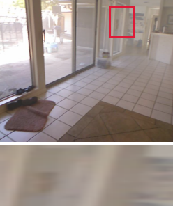
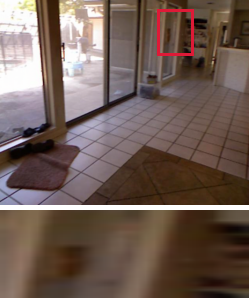
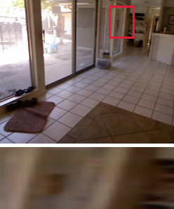
(a)Input	(b)MSBDN [12]	(c)FFA-Net [47]	(d)Dehamer [19]	(e)MAXIM [55]	(f)Dual-former	(g)Ground-truth

Figure 4: Visual comparisons of various deraining methods on SOTS-Indoor [31] dataset. Please zoom in for a better illustration.

III-C2 Multi-branch Feed Forward Network

As a vital part of the transformer block, the feed-forward network enriches the representation performance of the model. Previous architectures consist of multilayer perceptron (MLP), which limits the ability of the network to leverage the locally [43, 13]. ConvFFN [28, 58] applied depth-wise convolution to extract local contextual information. However, we note that in image restoration tasks, multi-scale information can better improve model performance due to its diverse receptive fields. Consequently, we propose the Multi-branch Feed-forward Network (MBFFN), which offers the different kernels of convolution to capture multi-size contextual information. As depicted in Fig.5, we first adopt 1$\times$1 convolution to expand the feature channels (we set expand factor $\beta$ = 2 to save computation in this paper). Next, we employ the multi-branch to aggregate different scale information by 3$\times$3 and 5$\times$5 convolution. Inspired by  [4], we use the Simple Gate (SG) operation to replace the GELU activation before the final 1$\times$1 convolution. Specifically, given an input $X\in\mathbb{R}^{H\times W\times C}$, our MBFFN can be formulated as:

$$Y=\operatorname{\varphi_{1}}(\operatorname{SG}(\operatorname{MB}(\operatorname{\varphi_{1}}(X))))+X,$$ (15)

$$\operatorname{MB}(X)=\operatorname{\varphi_{3}}(X)+\operatorname{\varphi_{5}}(X)+X,$$

where the $Y$ is the output feature.

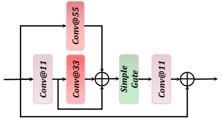
Figure 5: Architecture of Multi-branch Feed-forward Network.

III-C3 Parallel Local Feature Extract Module

In the HTB, besides the self-attention mechanism and feed-forward network, we also design a local feature extraction module in parallel with them along the channel dimension. It provides the ability of local information acquisition in high-dimensional space, which is complementary to the global modeling ability of the parallel hybrid self-attention mechanism. It is worth mentioning that we increase the highest number of dimensions due to the parallelism of the convolution blocks. However, compared with blocks composed of all transformers, our hybrid transformer block takes into account the balance between performance and computation, laying the foundation for the efficiency of the overall network.

III-D Loss Function

To facilitate our model for better image restoration performance. we utilize PSNR loss [5] as our reconstruction loss function. It can be expressed as follows:

$$\left.L_{psnr}=-\operatorname{PSNR}(I(X)),Y\right),$$ (16)

where PNSR($\cdot$) denotes the PSNR metrics, X and Y are the input and its corresponding ground-truth image, $I$($\cdot$) represents our Dual-former. In addition, we also use perceptual loss, which provides supervision at the perceptual perspective level:

$$L_{perceptual}=\sum_{j=1}^{2}\frac{1}{C_{j}H_{j}W_{j}}\left\|\phi_{j}(\mathcal{I}(X)\right)-\phi_{j}\left(Y)\right\|_{1},$$ (17)

wherein the $C_{j}$, $H_{j}$, $W_{j}$ are the number of channels, length and width of the feature map extracted in the j-th hidden feature of VGG19 [52] model, respectively. $\phi_{j}$ means the specified j-th layer of the network.

Therefore, our overall loss function can be expressed as follows:

$$L=\lambda_{1}L_{psnr}+\lambda_{2}L_{perceptual},$$ (18)

where $\lambda_{1}$ and $\lambda_{2}$ are set to 1 and 0.2 in our paper.

TABLE I: Deraining results on five datasets. Bold and underline indicate the best and the second best metrics.

Method	Test100 [68]		Rain100H [62]		Rain100L [62]		Test2800  [16]		Test1200 [67]		Average		#GFLOPs	#Param
	PSNR $\uparrow$	SSIM $\uparrow$	PSNR $\uparrow$	SSIM $\uparrow$	PSNR $\uparrow$	SSIM $\uparrow$	PSNR $\uparrow$	SSIM $\uparrow$	PSNR $\uparrow$	SSIM $\uparrow$	PSNR $\uparrow$	SSIM $\uparrow$
(TIP’17)DerainNet [15]	22.77	0.810	14.92	0.592	27.03	0.884	24.31	0.861	23.38	0.835	22.48	0.796	${88.287}$G	0.75M
(CVPR’18)DIDMDN [67]	22.56	0.818	17.35	0.524	25.23	0.741	28.13	0.867	29.65	0.901	24.58	0.770	$7.31G$	0.37K
(CVPR’19)UMRL [63]	24.41	0.829	26.01	0.832	29.18	0.923	29.97	0.905	30.55	0.910	28.02	0.880	16.50G	0.98K
(ECCV’18)RESCAN [34]	25.00	0.835	26.36	0.786	29.80	0.881	31.29	0.904	30.51	0.882	28.59	0.857	${32.32}$G	0.15M
(CVPR’19)PreNet [49]	24.81	0.851	26.77	0.858	32.44	0.950	31.29	0.904	30.51	0.882	29.42	0.897	${66.58}$G	0.17M
(CVPR’20)MSPFN [24]	27.50	0.876	28.66	0.860	32.40	0.933	31.75	0.916	31.36	0.911	30.75	0.903	708.44G	21.00M
(CVPR’21)MPRNet [66]	30.27	0.897	30.41	0.890	36.40	0.965	33.64	0.938	32.91	0.916	32.73	0.921	148.55G	3.64M
(CVPR’22)KiT [28]	30.26	0.904	30.47	0.897	36.65	0.969	33.85	0.941	32.81	0.918	32.81	0.926	43.08G	20.60M
Dual-former	$\mathbf{30.63}$	$\mathbf{0.908}$	$\mathbf{30.85}$	${0.894}$	$\mathbf{36.99}$	$\mathbf{0.969}$	${33.51}$	${0.937}$	32.66	$\mathbf{0.919}$	$\mathbf{32.93}$	$\mathbf{0.926}$	9.28G	14.23M

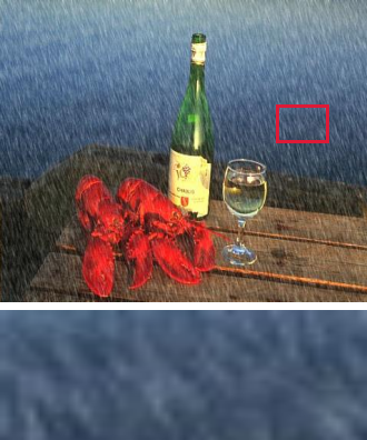
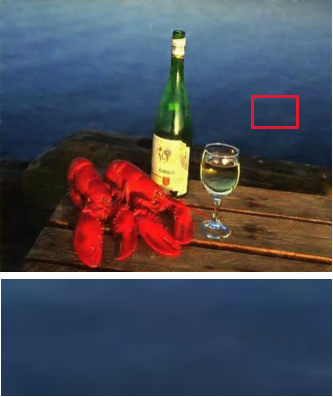
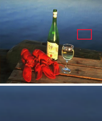
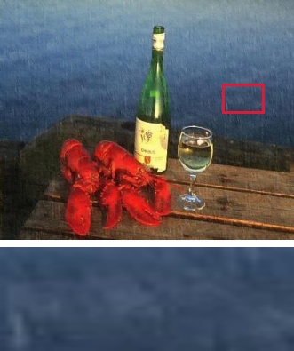
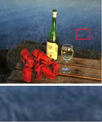
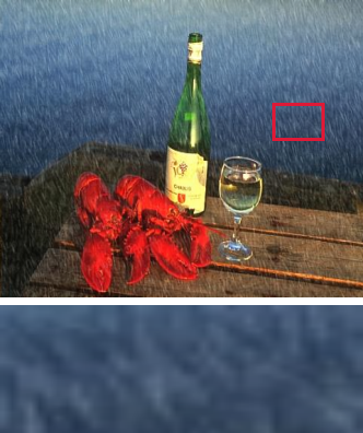
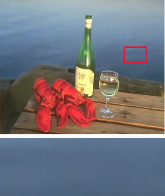
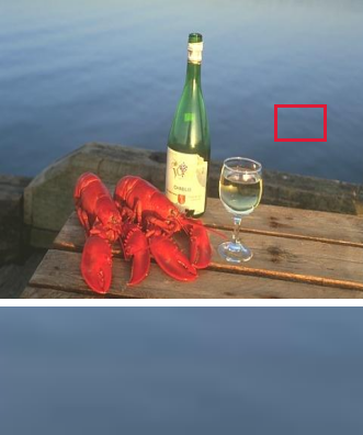
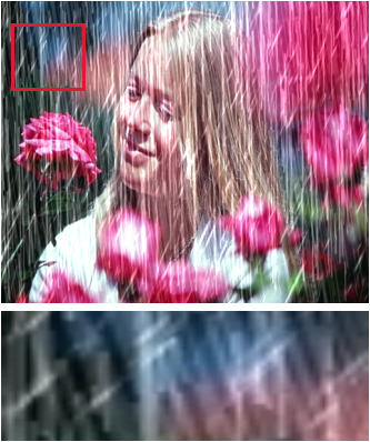
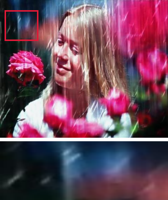
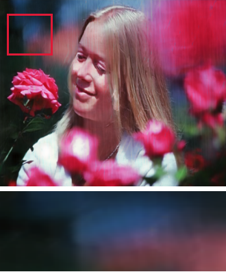
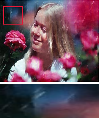
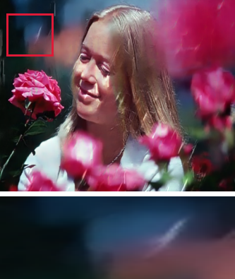
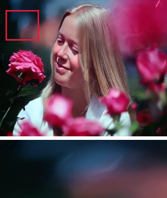
(a)Input	(b)DIDMDN [67]	(c)UMRL [63]	(d)RESCAN [34]	(e)PreNet [49]	(f)MPRNet [66]	(g)Dual-former	(h)Ground-truth

Figure 6: Visual comparisons of various deraining methods on Test100 [68] dataset. Please zoom it for a better illustration.

IV Experiments

IV-A Implementation Details

We train our model with the Adam optimizer, whose initial momentum is set to 0.9 and 0.999. We set the initial learning rate to be 0.0002 with cycle learning rate decay. We present 256$\times$256 patch size from the original image after data augmentation as our input and train them for 800 epochs for each low-level visual image restoration task. In terms of data augmentation, we flip horizontally and randomly rotate the image to a fixed angle. We choose the 1-th and 3-th layers of VGG19 [52] to adopt perceptual loss.

IV-B Architecture Design

For a concise description, we introduce the specific configurations of our Dual-former. We gradually expand the dimension of our encoder and set it to $\{$28, 32, 64, 128$\}$. We increase the number of LFE blocks for each encoder stage to $\{$4, 5, 7, 8$\}$. In the LFE block, we keep the original dimensions at the shallowest level and utilize the 1$\times$1 convolution to double the dimension numbers in other stages. In the latent layer, we increase the dimension numbers to 384 and stack 14 Hybrid Transformer Blocks to improve the network’s performance, whose number of multi-head is set to 8. At the same time, we follow the  [65] to apply the skip connection between the encoder and decoder.

IV-C Tasks and Metrics

Image restoration for severe weather is a challenging task (i.e., haze, rain, snow). Most previous models attract remarkable results in a single adverse weather restoration task. However, the performance in other tasks is not satisfactory. In this paper, we conduct extensive experiments on three adverse weather tasks and a total of ten datasets (Haze4K [39], SOTS [31], Test100 [68], Rain100H [62], Rain100L [62], Test2800 [15], Test1200 [67], CSD [8], SRRS [7] and Snow100K [41]) to verify the excellent property of Dual-former. For evaluation metrics, we adopt PSNR and SSIM [60] to be consistent with previous methods.

IV-D Image Dehazing

Image dehazing is a typical low-level vision task in image restoration for degraded weather. we compare the performance of Dual-former with other SOTA dehazing approaches: DCP [20], NLD [2], DehazeNet [3], GDN [38], MSBDN [12], DA [51], FFA-Net [47], DMT-Net [40], Dehamer [19] and MAXIM [55]. We train our Dual-former on Haze4K [39] dataset and ITS [31], the Haze4K testset [39] and SOTS-Indoor [31] as evaluation datasets to validate the restored performance.

Table II shows that our Dual-former achieves significant and unusual performance while keeping efficient characteristics due to its low GFLOPs compared with the state-of-the-art models. For the latest method (Dehamer and MAXIM), we exceed quantitative results by 1.91dB on SOTS-Indoor datasets compared with MAXIM, only using 4.2$\%$ computation (216.00G $\rightarrow$ 9.28G). In addition, we outperform the Dehamer substantially while adopting 10.7$\%$ parameters (132.45M $\rightarrow$ 14.23M). Fig.4 illustrates that the image produced by our design is superior in recovering details and overall effect, which is sharper and cleaner in local features than other state-of-the-art algorithms. To emphasize the impressive performance of image dehazing, we also present the visual comparison of real-world images in Fig.8. We catch that Dual-former attracts the non-trivial effect of removing the haze veiling from the degraded version. On the contrary, other SOTA approaches such as MAXIM and Dehamer, almost fail to recover the clean images.

TABLE II: Dehazing results on the Haze4K [40] and SOTS-Indoor [31] datasets. Bold and underline indicate the best and the second best metrics.

Method	Haze4k [40]		SOTS Indoor [31]		#GFLOPs	#Param
	PSNR $\uparrow$	SSIM $\uparrow$	PSNR $\uparrow$	SSIM $\uparrow$
(TPAMI’10)DCP [20]	$14.01$	$0.76$	$15.09$	$0.76$	$\mathbf{-}$	$\mathbf{-}$
(CVPR’16)NLD [2]	$15.27$	$0.67$	$17.27$	$0.75$	$\mathbf{-}$	$\mathbf{-}$
(TIP’16)DehazeNet [3]	$19.12$	$0.84$	$20.64$	$0.80$	0.52G	0.01M
(ICCV’17)GDN [38]	$23.29$	$0.93$	$32.16$	${0.98}$	21.49G	0.96M
(CVPR’20)MSBDN [12]	$22.99$	$0.85$	$33.79$	${0.98}$	41.58G	31.35M
(AAAI’20)FFA-Net [47]	$26.96$	$0.95$	$36.39$	$0.98$	288.34G	4.6M
(ACMMM’21)DMT-Net [40]	$\underline{28.53}$	$\underline{0.96}$	$\mathbf{-}$	$\mathbf{-}$	80.71G	54.9M
(CVPR’22)Dehamer [19]	$\mathbf{-}$	$\mathbf{-}$	36.63	0.99	59.15G	132.45M
(CVPR’22 Oral)MAXIM [55]	$\mathbf{-}$	$\mathbf{-}$	38.11	0.99	216.00G	14.10M
Dual-former	$\mathbf{32.85}$	$\mathbf{0.98}$	${\mathbf{40.02}}$	$\mathbf{0.99}$	9.28G	14.23M

IV-E Image Deraining

For the image deraining task, we follow the settings of most current mainstream methods [65], applying our Dual-former to train on multiple datasets, which include 13712 paired images. In the test stage, we evaluate the performance of our framework on five datasets, containing Rain100H [62], Rain100L [62], Test100 [68], Test2800 [16], and Test1200 [67]. We utilize PSNR and SSIM as our reference metrics and convert the image to Ycrcb color space to compute metrics for the Y channel, which is consistent with previous SOTA methods.

We present the compared results of the previous latest method in Table I. It’s noticed that most SOTA strategies for rain streak removal need massive computation to do more processing, which aims to cover the difference of five datasets such as MPRNet (148.55G) and KiT (43.08G). We outperform the latest approaches while only keeping the computation in the low overhead (9.28G). Fig.(6) is a visual comparison of other methods for the deraining task. We observe that our Dual-former can remove small rain streaks thoroughly instead of retaining a vestige of rain spots, especially in dense rain images where MPRNet almost fails to remove rain streaks. For the restored details, our approach is closer to the ground-truth. In a word, our manner has impressive visual effects compared with state-of-the-art methods. Furthermore, the deraining performance on the real-world dataset is also shown in Fig.8. We notice that the previous methods such as RESCAN[34] and MPRNet[66], remnant the large rain streaks in the restored image. Though PReNet[49] and MSPFN[24] can remove the lots of streaks, they are still hard to handle the residual rain spots perfectly. The image processed by Our Dual-former keeps the details while eliminating the rain degradations, which demonstrates that the proposed algorithm obtains dramatic performance on the real-world dataset.

TABLE III: Quantitative comparison of various desnowing approaches on the CSD [8], SRRS [7] and Snow 100K [41] datasets. Bold and underline indicate the best and the second best metrics.

Method	CSD (2000)		SRRS (2000)		Snow 100K (2000)		#GFLOPs	#Param
	PSNR $\uparrow$	SSIM $\uparrow$	PSNR $\uparrow$	SSIM $\uparrow$	PSNR $\uparrow$	SSIM $\uparrow$
(TIP’18)DesnowNet [41]	20.13	0.81	20.38	0.84	30.50	0.94	1.7KG	15.6M
(CVPR’18)CycleGAN [14]	20.98	0.80	20.21	0.74	26.81	0.89	42.38G	7.84M
(CVPR’20)All in One [32]	26.31	0.87	24.98	0.88	26.07	0.88	12.26G	44M
(ECCV’20)JSTASR [7]	27.96	0.88	25.82	0.89	23.12	0.86	-	65M
(ICCV’21)HDCW-Net [8]	29.06	0.91	27.78	0.92	31.54	0.95	9.78G	6.99M
(CVPR’22)TransWeather [56]	$\underline{31.76}$	$\underline{0.93}$	$\underline{28.29}$	$\underline{0.92}$	$\underline{31.82}$	${0.93}$	5.64G	21.9M
Dual-former	$\mathbf{35.90}$	$\mathbf{0.97}$	$\mathbf{\mathbf{32.92}}$	$\mathbf{0.96}$	$\mathbf{34.99}$	$\mathbf{0.97}$	9.28G	14.23M

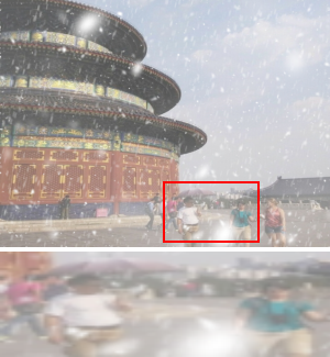
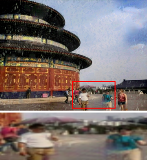
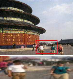
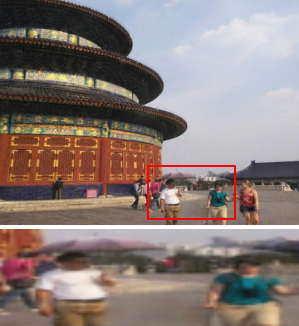
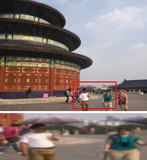
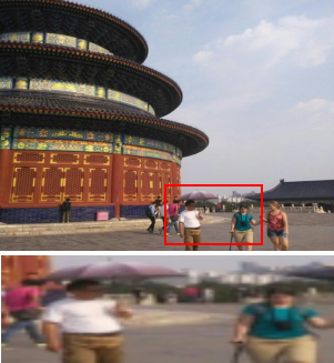
(a)Input	(b)JSTASR [7]	(c)HDCW-Net [8]	(d)TransWeather [56]	(e)Dual-former(Ours)	(f)Ground-truth

Figure 7: Visual comparison of our Dual-former and the state-of-the-art methods on the CSD [8] synthetic dataset . Please zoom it to watch the details better.

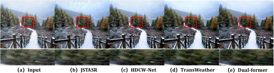
Figure 8: Visual comparison between adverse weather removal methods on real-world datasets (dehazing, deraining, desnowing). Please zoom them to watch the details better.

IV-F Image Desnowing

For single image snow removal, we train and test our Dual-former on three snow datasets, CSD [8] Snow100K [41], SRRS [7]. We follow the latest single image desnowing method [8] for training and testing on different testsets to ensure reasonableness and fairness (sample 2000 images from testset for each dataset). For the models without training on desnowing datasets, we re-train them and choose the best result for comparison.

The results of previous methods are shown in Table III. We notice that Dual-former shows substantial growth performance compared with state-of-the-art methods on CSD [8] datasets (31.76dB $\rightarrow$ 35.90dB), the same as SRRS [7] and Snow100K [41]. This excellent performance proves that our method is highly competitive in desnowing task. We also carry out the visual comparison, the effects are presented in Fig.7. From Fig.7, we found that our snow removal effect is better than the previous SOTA methods to remove various snow degradation and restore image color. At the same time, our Dual-former can better distinguish snow marks and object details while the HDCW-Net [8] and Transweather [56] almost recover failure. Furthermore, our features in the detailed enlarged image are more stunning and close to the ground-truth. We also compare the desnowing performance of SOTA manners on the real-world image, and the results are shown in Fig.8. We observe that previous methods JSTASR[7], HDCW-Net[8] and TransWeather[56] are difficult to resolve the small degradations, such as snow spots. However, Dual-former tackles this problem and has the best visual effect compared with the latest approaches.

IV-G Effective Receptive Field Analysis

Our main core design idea uses CNNs in the encoder part to extract local features, and embeds self-attention into latent to enhance the global modeling ability. Therefore, we employ the effective receptive (ERF) field [44] of different stages in the proposed architecture. From Fig.9, such ERF demonstrates that the LFE module in the encoder focuses on the local information extraction, while expanding the ERF progressively. In the latent layer, the hybrid transformer block performs global modeling primarily, which has a large ERF. Such a design fully considers the previous conclusions [48] while significantly reducing the computational overhead.

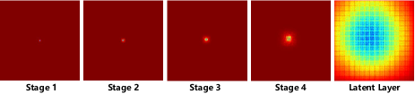
Figure 9: Effective Receptive Field of different stages on Rain100H [62] testset (average over 100 images).

IV-H Parameters and Computational complexity Analysis

In this section, we explore the advantages of Dual-former in parameters and computation. Parameters and FLOPs are within our scope of the designed architecture. Nevertheless, achieving impressive performance while keeping suitable parameters and computational overheads is challenging. In Table (II-I), We present the comparison results of the latest approaches in the different recovering tasks. We notice that our model’s computation is considerably less than most state-of-the-art methods. For image dehazing, we only use 4.2$\%$ computation complexity to surpass the MAXIM [55]’s performance. Furthermore, the amount of parameters is much less than most previous methods. It is worth mentioning that the parameter of FFA-Net [47] is 4.6M, while it needs a vast computational burden of 288.34G (256$\times 256$). Also, in the rain removal task, it is difficult for MPRNet [66] to balance the lightweight design while being a small computation.

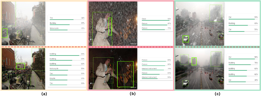
Figure 10: (a), (b) and (c) are the quantifiable performance for high-level vision tasks. The upper contents are the detection confidences of degraded images (haze, rain, snow) and the lower contents are the detection confidences of corresponding restored versions from Dual-former.

IV-I The merits of Dual-former

Inexpensive computation is introduced above, we further explore the merits of the overall architecture for Dual-former. We present the GFLOPs and time cost with respect to different image sizes in Fig.11. The growth rates of them are not sensitive to image resolutions compared with other SOTA methods such as Uformer [59] and MPRNet [66]. In other words, embedding ViT-based modules into hidden layers improves model performance without significantly increasing computational and time cost as the resolution changes. We can also observe that our speed and computational complexity are almost the lowest compared to the SOTA methods, demonstrating that our overall architecture achieves a balance between performance and computation for image restoration tasks and is more efficient for processing high-resolution images.

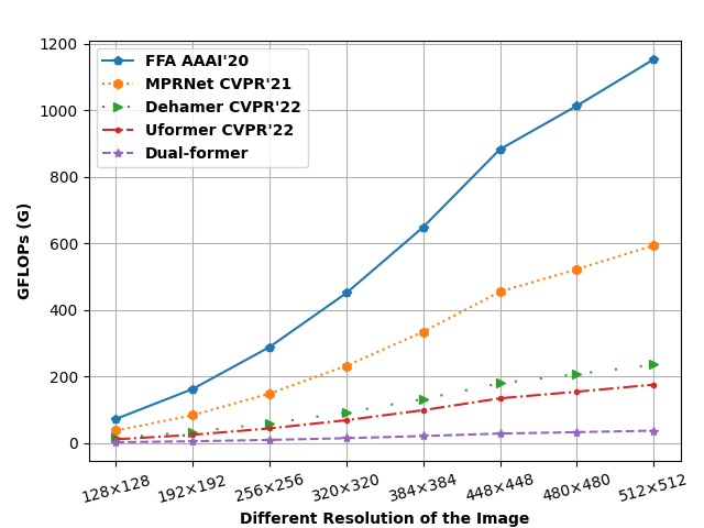
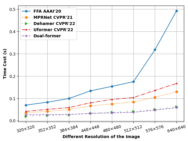
Figure 11: Left: GFLOPs of our method and SOTA methods with respect to different image resolutions. Our Dual-former has fewer GFLOPs than all competitors, and it enjoys the lowest GFLOPs growth rate inspired by input image size. Right: Time cost corresponding to various input image sizes of proposed Dual-former and SOTA approaches. Dual-former is superior in time cost compared with almost previous methods, and it achieves less speed cost with increasing image resolution compared to the latest Vit-based image architecture Uformer.

IV-J Quantifiable Performance for High-level Vision Tasks

As shown in Fig.10, we present the detection confidences supported by Google Vision API. From Fig.10, we notice that the degraded information affects the detection results to some extent. Specifically, haze, rain and snow reduce the objection numbers and confidences of detection, which limits the performance of high-level vision tasks. After processing by Dual-former, the restored image can tackle this problem and promote the development of high-level tasks.

IV-K Ablation Study

In this section, we conduct extensive ablation studies to verify the effect of our Dual-former network design. Specifically, we adopt the 192$\times$192 patch size of images on CSD [8] training set as input and train 200 epochs. Then we observe the results on CSD [8] testing dataset to analyze crucial components. We illustrate the influence of each composition in the following parts individually.

IV-K1 Effectiveness of Channel-Spatial Self-attention

We first verify the effect of our Channel-Spatial Self-attention, which differs from other single dimensional perspective self-attention such as channel level [65] or spatial level [13]. We perform the following experiments on validating the superior of multi-perspective self-attention compared with other self-attention. (a) We replace the Channel-Spatial Self-attention with the self-attention module inspired by vanilla Transformer [13] (SSA). (b) we explore the gain of depth-wise convolution in spatial self-attention operation.(c) We apply self-attention across channel [65] to substitute our Hybrid Self-attention design (CSA). (d) We use Channel-Spatial Self-attention operation in our architecture (CSSA). Table IV reports comparison results for different configurations. We observe that Channel-Spatial Self-attention can provide a better representation to recover degraded images, which we believe can be explained by global modeling from both channel and spatial levels are more powerful than single self-attention for image restoration. And the depth-wise can enhance the local bias in spatial self-information.

TABLE IV: Ablation Study on Self-attention of different dimensional perspectives. Underline indicates the best metrics. (PSNR(dB)/SSIM)

Setting	Model	#Param	#GFLOPs	PSNR	SSIM
a	SSA	14.21M	9.27G	30.21	0.936
b	SSA wo DWConv	14.21M	9.26G	30.06	0.933
c	CSA	14.26M	9.28G	30.36	0.937
d	CSSA(Ours)	14.23M	9.28G	30.64	0.939

IV-K2 Novelty for Multi-branch feed-forward network (MBFFN)

In this article, we propose the MBFFN instead of Multilayer Perceptron (MLP) [43] for image restoration of various severe weather datasets. To demonstrate that MBFFN outperforms previous feed-forward network (FFN) designs, we modify the multiple experiments of FFN, which can further prove the obtained gain from MBFFN. (a) We follow the MLP as FFN backbone just like [43] (MLP). (b) In the PVT [58], authors present the ConvFFN to improve the local excavation capacity. We compare it in image restoration to observe their performance [28] (ConvFFN). (c) We also compare with LeFF module [59] in this part, which attracts the remarkable results in image restoration field (LeFF). (d) We use MBFFN to replace the above designs (MFFN). Table V verifies that MBFFN can achieve non-trivial than other variants of FFN in transformer block. Our MBFFN cancels the FC layers and changes to apply convolution. Multi-branch operation enhances the multi-scale local representation ability, which is complementary to self-attention.

TABLE V: Ablation Study on various configurations of Feed-forward Network. Underline indicates the best metrics. (PSNR(dB)/SSIM)

Setting	Model	#Param	#GFLOPs	PSNR	SSIM
a	MLP [43]	14.56M	9.36G	30.37	0.937
b	ConvFFN [28]	14.61M	9.37G	30.42	0.938
c	LeFF [59]	14.61M	9.39G	30.53	0.938
d	MFFN(Ours)	14.23M	9.28G	30.64	0.939

IV-K3 Benefits of Adaptive Control Module

To enhance the interaction of hybrid self-attention (Channel-Spatial Self-attention), we carefully introduce the Adaptive Control Module (ACM), which offsets the shortcoming of different dimensional perspectives to fuse the information ideally. We conduct ablation studies to explore various ways of modulating and their gains. (a) Without any Adaptive Control Module, only using concatenate operation to substitute it (Concat). (b) We follow the  [53] inspired by [35], testing the SK fusion to fuse multiple branches. (c) We use the Adaptive Control Module (ACM) to replace other modules. Compared with SK fusion and concatenate operation, our ACM requires more computation and parameters, while instead, it has better performance in PSNR and SSIM. This increase is within the acceptable range compared to the computational cost. It demonstrates that our ACM improves the capability of fusing the information from the channel and spatial levels, leading to superior performance over SK fusion and simple concatenation.

TABLE VI: Ablation Study on different information fusion operations. Underline indicates the best metrics. (PSNR(dB)/SSIM)

Setting	Model	#Param	#GFLOPs	PSNR	SSIM
a	Concat	9.78M	8.76G	30.03	0.932
b	SK fusion [53]	9.82M	8.76G	30.12	0.933
c	ACM(Ours)	14.23M	9.28G	30.64	0.939

IV-K4 Necessity of Channel Attention (CA) in Local Feature Extraction Block (LFE)

For the proposed LFE, we embed channel attention to consolidate the information exchange between channel dimensions, improving the overall performance in the encoder-decoder part. The detailed experiments are shown in Table VII. It’s worth that we notice that the channel attention brings a certain degree of effect, while The amount of computation and parameters only rise a little ($\mathbf{9.24G\rightarrow 9.28G}$ and $\mathbf{12.52M\rightarrow 14.28M}$). This conclusion reflects that channel attention plays a vital role in our purpose.

TABLE VII: Ablation Study on Channel Attention in Local Feature Extraction module and Hybrid Transformer Block with LFE module. Underline indicates the best metrics. (PSNR(dB)/SSIM)

LFE w CA	$\#$Param	$\#$GFLOPs	PSNR	SSIM
✗	12.52M	9.24G	30.22	0.934
✓	14.23M	9.28G	30.64	0.939
HTB w LFE	$\#$Param	$\#$GFLOPs	PSNR	SSIM
✗	11.01M	8.71G	30.04	0.932
✓	14.23M	9.28G	30.64	0.939

IV-K5 Benefits of Local Feature Extraction in Hybrid Transformer Block

In the latent layer of the network, we design a parallel architecture to utilize a subset of channels for our local feature extraction. It can complement another part of the global modeling information to enhance the ability in the deepest layer, thereby improving the model’s overall performance. In this ablation experiment, we demonstrate the effectiveness of this design. It can be seen from Table VII that this parallelized design dramatically enhances the overall image restoration capability of the model and maintains a small computational cost.

IV-K6 Effectiveness of Loss Function

In this ablation study, we explore the effectiveness of our chosen loss function. We apply the PSNRloss [5] as our reconstruction loss instead of L1 loss. At the same time, we study to prove the effect of perceptual loss in our train setting. Table VIII describes that PSNRloss has a slight advantage over L1 loss, perceptual loss is helpful during training due to its supervision at the feature level.

TABLE VIII: Ablation Study on the effect of the loss function. Underline indicates the best metrics. (PSNR(dB)/SSIM)

Setting	Model	PSNR	SSIM
1	$L1+L_{p}$	30.57	0.939
2	$L_{psnr}$	30.34	0.936
3	$L_{p}+L_{psnr}$ (Ours)	30.64	0.939

V Conclusion

In this paper, we have proposed a powerful yet efficient image restoration backbone. In contrast to Transformer-based image restoration structures, we only embed the Hybrid Transformer Block into the latent layer to unleash its mighty global modeling capabilities. This design cleverly combines the ability of local extraction and global information interaction while possessing low computational complexity compared to existing large networks. Experiments show the superiority of our Dual-former consisting of Local Feature Extraction and Hybrid Transformer Block (Channel-Spatial Self-attention), which presents strong representation capability for different adverse weather restoration tasks. We hope our backbone can be used for other efficient and robust network designs and achieve impressive results in numerous fields, such as image super-resolution and image demoiring.

References

- [1] A. Abuolaim and M. S. Brown, “Defocus deblurring using dual-pixel data,” in European Conference on Computer Vision. Springer, 2020, pp. 111–126.
- [2] D. Berman, S. Avidan et al., “Non-local image dehazing,” in Proceedings of the IEEE conference on computer vision and pattern recognition, 2016, pp. 1674–1682.
- [3] B. Cai, X. Xu, K. Jia, C. Qing, and D. Tao, “Dehazenet: An end-to-end system for single image haze removal,” IEEE Transactions on Image Processing, vol. 25, no. 11, pp. 5187–5198, 2016.
- [4] L. Chen, X. Chu, X. Zhang, and J. Sun, “Simple baselines for image restoration,” arXiv preprint arXiv:2204.04676, 2022.
- [5] L. Chen, X. Lu, J. Zhang, X. Chu, and C. Chen, “Hinet: Half instance normalization network for image restoration,” in Proceedings of the IEEE/CVF Conference on Computer Vision and Pattern Recognition, 2021, pp. 182–192.
- [6] S. Chen, T. Ye, Y. Liu, E. Chen, J. Shi, and J. Zhou, “Snowformer: Scale-aware transformer via context interaction for single image desnowing,” arXiv preprint arXiv:2208.09703, 2022.
- [7] W.-T. Chen, H.-Y. Fang, J.-J. Ding, C.-C. Tsai, and S.-Y. Kuo, “Jstasr: Joint size and transparency-aware snow removal algorithm based on modified partial convolution and veiling effect removal,” in European Conference on Computer Vision. Springer, 2020, pp. 754–770.
- [8] W.-T. Chen, H.-Y. Fang, C.-L. Hsieh, C.-C. Tsai, I. Chen, J.-J. Ding, S.-Y. Kuo et al., “All snow removed: Single image desnowing algorithm using hierarchical dual-tree complex wavelet representation and contradict channel loss,” in Proceedings of the IEEE/CVF International Conference on Computer Vision, 2021, pp. 4196–4205.
- [9] Y. Chen, X. Dai, D. Chen, M. Liu, X. Dong, L. Yuan, and Z. Liu, “Mobile-former: Bridging mobilenet and transformer,” arXiv preprint arXiv:2108.05895, 2021.
- [10] S.-J. Cho, S.-W. Ji, J.-P. Hong, S.-W. Jung, and S.-J. Ko, “Rethinking coarse-to-fine approach in single image deblurring,” in Proceedings of the IEEE/CVF international conference on computer vision, 2021, pp. 4641–4650.
- [11] T. Dai, J. Cai, Y. Zhang, S.-T. Xia, and L. Zhang, “Second-order attention network for single image super-resolution,” in Proceedings of the IEEE/CVF conference on computer vision and pattern recognition, 2019, pp. 11 065–11 074.
- [12] H. Dong, J. Pan, L. Xiang, Z. Hu, X. Zhang, F. Wang, and M.-H. Yang, “Multi-scale boosted dehazing network with dense feature fusion,” in Proceedings of the IEEE/CVF conference on computer vision and pattern recognition, 2020, pp. 2157–2167.
- [13] A. Dosovitskiy, L. Beyer, A. Kolesnikov, D. Weissenborn, X. Zhai, T. Unterthiner, M. Dehghani, M. Minderer, G. Heigold, S. Gelly et al., “An image is worth 16x16 words: Transformers for image recognition at scale,” arXiv preprint arXiv:2010.11929, 2020.
- [14] D. Engin, A. Genç, and H. Kemal Ekenel, “Cycle-dehaze: Enhanced cyclegan for single image dehazing,” in Proceedings of the IEEE conference on computer vision and pattern recognition workshops, 2018, pp. 825–833.
- [15] X. Fu, J. Huang, X. Ding, Y. Liao, and J. Paisley, “Clearing the skies: A deep network architecture for single-image rain removal,” IEEE Transactions on Image Processing, vol. 26, no. 6, pp. 2944–2956, 2017.
- [16] X. Fu, J. Huang, D. Zeng, Y. Huang, X. Ding, and J. Paisley, “Removing rain from single images via a deep detail network,” in Proceedings of the IEEE conference on computer vision and pattern recognition, 2017, pp. 3855–3863.
- [17] Z. Fu, X. Lin, W. Wang, Y. Huang, and X. Ding, “Underwater image enhancement via learning water type desensitized representations,” in ICASSP 2022-2022 IEEE International Conference on Acoustics, Speech and Signal Processing (ICASSP). IEEE, 2022, pp. 2764–2768.
- [18] B. Graham, A. El-Nouby, H. Touvron, P. Stock, A. Joulin, H. Jégou, and M. Douze, “Levit: a vision transformer in convnet’s clothing for faster inference,” in Proceedings of the IEEE/CVF International Conference on Computer Vision, 2021, pp. 12 259–12 269.
- [19] C.-L. Guo, Q. Yan, S. Anwar, R. Cong, W. Ren, and C. Li, “Image dehazing transformer with transmission-aware 3d position embedding,” in Proceedings of the IEEE/CVF Conference on Computer Vision and Pattern Recognition (CVPR), June 2022, pp. 5812–5820.
- [20] K. He, J. Sun, and X. Tang, “Single image haze removal using dark channel prior,” IEEE transactions on pattern analysis and machine intelligence, vol. 33, no. 12, pp. 2341–2353, 2010.
- [21] K. He, X. Zhang, S. Ren, and J. Sun, “Deep residual learning for image recognition,” in Proceedings of the IEEE conference on computer vision and pattern recognition, 2016, pp. 770–778.
- [22] J. Hu, L. Shen, and G. Sun, “Squeeze-and-excitation networks,” in Proceedings of the IEEE conference on computer vision and pattern recognition, 2018, pp. 7132–7141.
- [23] J.-J. Huang and P. L. Dragotti, “Winnet: Wavelet-inspired invertible network for image denoising,” IEEE Transactions on Image Processing, 2022.
- [24] K. Jiang, Z. Wang, P. Yi, C. Chen, B. Huang, Y. Luo, J. Ma, and J. Jiang, “Multi-scale progressive fusion network for single image deraining,” in Proceedings of the IEEE/CVF conference on computer vision and pattern recognition, 2020, pp. 8346–8355.
- [25] Y. Jin, A. Sharma, and R. T. Tan, “Dc-shadownet: Single-image hard and soft shadow removal using unsupervised domain-classifier guided network,” in Proceedings of the IEEE/CVF International Conference on Computer Vision, 2021, pp. 5027–5036.
- [26] Y. Jin, W. Yang, and R. T. Tan, “Unsupervised night image enhancement: When layer decomposition meets light-effects suppression,” arXiv preprint arXiv:2207.10564, 2022.
- [27] O. Kupyn, T. Martyniuk, J. Wu, and Z. Wang, “Deblurgan-v2: Deblurring (orders-of-magnitude) faster and better,” in Proceedings of the IEEE/CVF International Conference on Computer Vision, 2019, pp. 8878–8887.
- [28] H. Lee, H. Choi, K. Sohn, and D. Min, “Knn local attention for image restoration,” in Proceedings of the IEEE/CVF Conference on Computer Vision and Pattern Recognition, 2022, pp. 2139–2149.
- [29] J. Lee, H. Son, J. Rim, S. Cho, and S. Lee, “Iterative filter adaptive network for single image defocus deblurring,” in Proceedings of the IEEE/CVF Conference on Computer Vision and Pattern Recognition, 2021, pp. 2034–2042.
- [30] Y. Lee, J. Kim, J. Willette, and S. J. Hwang, “Mpvit: Multi-path vision transformer for dense prediction,” arXiv preprint arXiv:2112.11010, 2021.
- [31] B. Li, W. Ren, D. Fu, D. Tao, D. Feng, W. Zeng, and Z. Wang, “Benchmarking single-image dehazing and beyond,” IEEE Transactions on Image Processing, vol. 28, no. 1, pp. 492–505, 2018.
- [32] R. Li, R. T. Tan, and L.-F. Cheong, “All in one bad weather removal using architectural search,” in Proceedings of the IEEE/CVF Conference on Computer Vision and Pattern Recognition, 2020, pp. 3175–3185.
- [33] X. Li, J. Wu, Z. Lin, H. Liu, and H. Zha, “Recurrent squeeze-and-excitation context aggregation net for single image deraining,” in Proceedings of the European conference on computer vision (ECCV), 2018, pp. 254–269.
- [34] ——, “Recurrent squeeze-and-excitation context aggregation net for single image deraining,” in Proceedings of the European conference on computer vision (ECCV), 2018, pp. 254–269.
- [35] X. Li, W. Wang, X. Hu, and J. Yang, “Selective kernel networks,” in Proceedings of the IEEE/CVF conference on computer vision and pattern recognition, 2019, pp. 510–519.
- [36] Y. Li, K. Zhang, R. Timofte, L. Van Gool, F. Kong, M. Li, S. Liu, Z. Du, D. Liu, C. Zhou et al., “Ntire 2022 challenge on efficient super-resolution: Methods and results,” in Proceedings of the IEEE/CVF Conference on Computer Vision and Pattern Recognition, 2022, pp. 1062–1102.
- [37] J. Liang, J. Cao, G. Sun, K. Zhang, L. Van Gool, and R. Timofte, “Swinir: Image restoration using swin transformer,” in Proceedings of the IEEE/CVF International Conference on Computer Vision, 2021, pp. 1833–1844.
- [38] X. Liu, Y. Ma, Z. Shi, and J. Chen, “Griddehazenet: Attention-based multi-scale network for image dehazing,” in Proceedings of the IEEE/CVF International Conference on Computer Vision, 2019, pp. 7314–7323.
- [39] Y. Liu, L. Zhu, S. Pei, H. Fu, J. Qin, Q. Zhang, L. Wan, and W. Feng, “From synthetic to real: Image dehazing collaborating with unlabeled real data,” in Proceedings of the 29th ACM International Conference on Multimedia, 2021, pp. 50–58.
- [40] ——, “From synthetic to real: Image dehazing collaborating with unlabeled real data,” in Proceedings of the 29th ACM International Conference on Multimedia, 2021, pp. 50–58.
- [41] Y.-F. Liu, D.-W. Jaw, S.-C. Huang, and J.-N. Hwang, “Desnownet: Context-aware deep network for snow removal,” IEEE Transactions on Image Processing, vol. 27, no. 6, pp. 3064–3073, 2018.
- [42] Z. Liu, H. Hu, Y. Lin, Z. Yao, Z. Xie, Y. Wei, J. Ning, Y. Cao, Z. Zhang, L. Dong et al., “Swin transformer v2: Scaling up capacity and resolution,” in Proceedings of the IEEE/CVF Conference on Computer Vision and Pattern Recognition, 2022, pp. 12 009–12 019.
- [43] Z. Liu, Y. Lin, Y. Cao, H. Hu, Y. Wei, Z. Zhang, S. Lin, and B. Guo, “Swin transformer: Hierarchical vision transformer using shifted windows,” in Proceedings of the IEEE/CVF International Conference on Computer Vision, 2021, pp. 10 012–10 022.
- [44] W. Luo, Y. Li, R. Urtasun, and R. Zemel, “Understanding the effective receptive field in deep convolutional neural networks,” Advances in neural information processing systems, vol. 29, 2016.
- [45] S. Mehta and M. Rastegari, “Mobilevit: light-weight, general-purpose, and mobile-friendly vision transformer,” arXiv preprint arXiv:2110.02178, 2021.
- [46] T. Pang, H. Zheng, Y. Quan, and H. Ji, “Recorrupted-to-recorrupted: unsupervised deep learning for image denoising,” in Proceedings of the IEEE/CVF conference on computer vision and pattern recognition, 2021, pp. 2043–2052.
- [47] X. Qin, Z. Wang, Y. Bai, X. Xie, and H. Jia, “Ffa-net: Feature fusion attention network for single image dehazing,” in Proceedings of the AAAI Conference on Artificial Intelligence, vol. 34, no. 07, 2020, pp. 11 908–11 915.
- [48] M. Raghu, T. Unterthiner, S. Kornblith, C. Zhang, and A. Dosovitskiy, “Do vision transformers see like convolutional neural networks?” Advances in Neural Information Processing Systems, vol. 34, pp. 12 116–12 128, 2021.
- [49] D. Ren, W. Zuo, Q. Hu, P. Zhu, and D. Meng, “Progressive image deraining networks: A better and simpler baseline,” in Proceedings of the IEEE/CVF Conference on Computer Vision and Pattern Recognition, 2019, pp. 3937–3946.
- [50] O. Ronneberger, P. Fischer, and T. Brox, “U-net: Convolutional networks for biomedical image segmentation,” in International Conference on Medical image computing and computer-assisted intervention. Springer, 2015, pp. 234–241.
- [51] Y. Shao, L. Li, W. Ren, C. Gao, and N. Sang, “Domain adaptation for image dehazing,” in Proceedings of the IEEE/CVF conference on computer vision and pattern recognition, 2020, pp. 2808–2817.
- [52] K. Simonyan and A. Zisserman, “Very deep convolutional networks for large-scale image recognition,” arXiv preprint arXiv:1409.1556, 2014.
- [53] Y. Song, Z. He, H. Qian, and X. Du, “Vision transformers for single image dehazing,” arXiv preprint arXiv:2204.03883, 2022.
- [54] H. Su, L. Yu, and C. Jung, “Joint contrast enhancement and noise reduction of low light images via jnd transform,” IEEE Transactions on Multimedia, 2020.
- [55] Z. Tu, H. Talebi, H. Zhang, F. Yang, P. Milanfar, A. Bovik, and Y. Li, “Maxim: Multi-axis mlp for image processing,” in Proceedings of the IEEE/CVF Conference on Computer Vision and Pattern Recognition, 2022, pp. 5769–5780.
- [56] J. M. J. Valanarasu, R. Yasarla, and V. M. Patel, “Transweather: Transformer-based restoration of images degraded by adverse weather conditions,” in Proceedings of the IEEE/CVF Conference on Computer Vision and Pattern Recognition, 2022, pp. 2353–2363.
- [57] A. Vaswani, N. Shazeer, N. Parmar, J. Uszkoreit, L. Jones, A. N. Gomez, Ł. Kaiser, and I. Polosukhin, “Attention is all you need,” Advances in neural information processing systems, vol. 30, 2017.
- [58] W. Wang, E. Xie, X. Li, D.-P. Fan, K. Song, D. Liang, T. Lu, P. Luo, and L. Shao, “Pyramid vision transformer: A versatile backbone for dense prediction without convolutions,” in Proceedings of the IEEE/CVF International Conference on Computer Vision, 2021, pp. 568–578.
- [59] Z. Wang, X. Cun, J. Bao, W. Zhou, J. Liu, and H. Li, “Uformer: A general u-shaped transformer for image restoration,” in Proceedings of the IEEE/CVF Conference on Computer Vision and Pattern Recognition, 2022, pp. 17 683–17 693.
- [60] Z. Wang, A. C. Bovik, H. R. Sheikh, and E. P. Simoncelli, “Image quality assessment: from error visibility to structural similarity,” IEEE transactions on image processing, vol. 13, no. 4, pp. 600–612, 2004.
- [61] H. Wu, B. Xiao, N. Codella, M. Liu, X. Dai, L. Yuan, and L. Zhang, “Cvt: Introducing convolutions to vision transformers,” in Proceedings of the IEEE/CVF International Conference on Computer Vision, 2021, pp. 22–31.
- [62] W. Yang, R. T. Tan, J. Feng, J. Liu, Z. Guo, and S. Yan, “Deep joint rain detection and removal from a single image,” in Proceedings of the IEEE conference on computer vision and pattern recognition, 2017, pp. 1357–1366.
- [63] R. Yasarla and V. M. Patel, “Uncertainty guided multi-scale residual learning-using a cycle spinning cnn for single image de-raining,” in Proceedings of the IEEE/CVF Conference on Computer Vision and Pattern Recognition, 2019, pp. 8405–8414.
- [64] T. Ye, M. Jiang, Y. Zhang, L. Chen, E. Chen, P. Chen, and Z. Lu, “Perceiving and modeling density is all you need for image dehazing,” arXiv preprint arXiv:2111.09733, 2021.
- [65] S. W. Zamir, A. Arora, S. Khan, M. Hayat, F. S. Khan, and M.-H. Yang, “Restormer: Efficient transformer for high-resolution image restoration,” arXiv preprint arXiv:2111.09881, 2021.
- [66] S. W. Zamir, A. Arora, S. Khan, M. Hayat, F. S. Khan, M.-H. Yang, and L. Shao, “Multi-stage progressive image restoration,” in Proceedings of the IEEE/CVF Conference on Computer Vision and Pattern Recognition, 2021, pp. 14 821–14 831.
- [67] H. Zhang and V. M. Patel, “Density-aware single image de-raining using a multi-stream dense network,” in Proceedings of the IEEE conference on computer vision and pattern recognition, 2018, pp. 695–704.
- [68] H. Zhang, V. Sindagi, and V. M. Patel, “Image de-raining using a conditional generative adversarial network,” IEEE transactions on circuits and systems for video technology, vol. 30, no. 11, pp. 3943–3956, 2019.
- [69] H. Zhao, Y. Zhang, S. Liu, J. Shi, C. C. Loy, D. Lin, and J. Jia, “Psanet: Point-wise spatial attention network for scene parsing,” in Proceedings of the European conference on computer vision (ECCV), 2018, pp. 267–283.