An analogue of the Kauffman bracket polynomial for knots in the non-orientable thickening of a non-orientable surface

Abstract.

We consider pseudo-classical knots in the non-orientable thickening of a non-orientable surface, i.e., knots which are orientation-preserving paths in a non-orientable $3$-manifold of the form (a non-orientable surface) $\times$ $[0,1]$. For this kind of knots we propose an analog of the Kauffman bracket polynomial. The construction of the polynomial is very close to its classical prototype, the difference consists in the using a new definition of the sign of a crossing and a new definition of positive/negative smoothings of a crossing. We prove that the polynomial is an isotopy invariant of pseudo classical knots and show that the invariant is not a consequence of the classical Kauffman bracket polynomial for knots in thickened orientable surface which is the orientable double cover of the non-orientable surface under consideration.

Key words: knots in non-orientable manifold, knots in thickened surface, pseudo-classical knots, Kauffman bracket polynomial

Introduction

Initially the theory of knots studied knots in $3$-sphere, but now many other kinds of objects are also considered in the theory. In the context of present paper first of all we need to mention knots in a thickened surface, i.e., in an orientable $3$-manifold of the form the direct product of a closed orientable surface and a segment. Some authors consider the case of knots in thickened non-orientable surface ([1],[2],[6],[11]) where the thickening is understood as an orientable $3$-manifold equipped with an $I$-bundle structure (here $I$ denotes a segment) over a surface which is not necessarily orientable. Note that in all these cases the thickening is assumed to be orientable independently whether the base surface is orientable or not.

Knots in non-orientable $3$-manifolds are studied also (see, for example, [13], [14]) but, unfortunately, the subject is not very popular. Maybe, one of reasons is that some important constructions cannot be transfered straightforwardly from orientable to non-orientable case. In particular, that is so for the Kauffman bracket polynomial ([7],[8]) and many other polynomial knot invariants which explicitly use in their construction the notion of the sign of a crossing (see, for example, [5],[9],[12],[10]) In the classical situation the sign of a crossing $x$ of an oriented diagram $D$ in a surface $\Sigma$ is defined to be $1$ (resp. $-1$) if a pair (a positive tangent vector of overgoing branch at $x$, a positive tangent vector of undergoing branch at $x$) is a positive (resp. negative) basis in the tangent space of $\Sigma$ at $x$. Clearly, the definition cannot be used if $\Sigma$ is non-orientable. One more example is the notion of positive and negative smoothing of a crossing (in other terms, the smoothing of the type $a$ and of the type $b$) playing a key role in the construction of the Kauffman bracket polynomial. The definition of the latter notion uses concepts of “right” and “left” which have no sense on a non-orientable surface. Note that aforementioned notions can be reformulated so that they have sense in the case of orientable thickening of non-orientable surface but the approach allowing to do this cannot be used in the case of non-orientable thickening of non-orientable surface.

In present paper we consider knots in the non-orientable thickening of a non-orientable surface, i.e., in a non-orientable $3$-manifold of the form $\Sigma\times[0,1]$ where $\Sigma$ is a non-orientable surface with (maybe) non-empty boundary. We propose an approach which in some particular case gives a correct definitions of the sign of a crossing and of two types of a smoothing. The knots we mean (we call them pseudo-classical) are those which are orientation-preserving paths in the manifold. Having two aforementioned definitions we define an analog of the Kauffman bracket polynomial for pseudo-classical knots. The construction we use word-for-word coincides with the classical one, the specificity of the non-orientable thickening is hidden in using definition of positive and negative smoothing. Our proof of the invariance of the polynomial (we denote it by $J$) is close to the classical one but do not coincide with the latter. Finally we compare the polynomial $J$ with its natural competitor — with the Kauffman bracket polynomial for knots in thickened orientable surface which is the orientable double cover of the non-orientable surface under consideration. We show that none of these invariants is a consequence of the other. Namely, we consider two pairs of knots in the non-orientable thickening of the Klein bottle so that knots forming the first pair have coinciding polynomials $J$ while $2$-component links in the thickened torus which are their double covers have distinct Kauffman bracket polynomials. Knots forming the second pair, on the contrary, have distinct polynomials $J$ while their double covers have coinciding Kauffman bracket polynomials.

The paper is organized as follows. In Section 1 we give some definitions including new definition of the sign of a crossing. In Section 2 we define two types of smoothing. Then we define the polynomial $J$ and prove its invariance. In the end of this section we briefly discuss a generalization of the polynomial analogous to the homological version of the Kauffman bracket polynomial for knots in a thickened orientable surface  [3]. In Section 3 we compare the polynomial $J$ and the Kauffman bracket polynomial for orientable double cover. In particular, in Section 3.2 we explicitly compute the polynomial $J$ for two knots in the non-orientable thickening of the Klein bottle. In Appendix we give source data needed for computing the values of the Kauffman bracket polynomial in the format acceptable by the computer program “3–manifold recognizer”.

1. Definitions

1.1. Knots and diagrams

Throughout $\Sigma$ denotes a non-orientable surface with (maybe) non-empty boundary and $\hat{\Sigma}$ denotes the non-orientable manifold of the form $\Sigma\times[0,1]$ with fixed structure of the direct product. The latter condition becomes crucial for us in the case of surface with non-empty boundary when there are aforementioned structures of the corresponding manifold with homeomorphic but non-isotopic base surfaces.

Knots in $\hat{\Sigma}$ and their diagrams in $\Sigma$ can be defined by analogy with the case of knots in a thickened orientable surface (below we will refer the latter case as the “classical case”). Knots in $\hat{\Sigma}$ will be considered up to isotopy.

In our case two diagrams on $\Sigma$ represent the same knot if and only if they are connected by a finite sequence of Reidemeister moves $R_{1},R_{2},R_{3}$ (which are just the same as classical ones) and ambient isotopies. indeed, let $\Sigma$ be represented by polygon of which sides are assumed to be identified (maybe) with a twist and a diagram is drawn inside the polygon. If we isotope the knot inquestion inside the direct product of the polygon and the segment then we can refer the corresponding classical fact. Otherwise it is necessary to consider a few auxiliary moves. The moves describe how we can push arcs and crossings of the diagrams through the boundary of the polygon. In the case of knots in orientable thickening of non-orientable surface (see, for example, [2], [1]) some of these moves permute overgoing and undergoing branches at moving crossing. In our case $\hat{\Sigma}$ is the direct product hance we have no moves permuting overgoing and undergoing branches, i.e., all auxiliary moves represent ambient isotopies of a diagram. Therefore, in proofs below we can restrict ourselves to Reidemeister moves $R_{1},R_{2},R_{3}$.

1.2. Pseudo-classical knots

A knot $K\subset\hat{\Sigma}$ is called an pseudo-classical if it is an orientation preserving path in $\hat{\Sigma}$. In other words, a knot in $\hat{\Sigma}$ is pseudo-classical if its regular neighbourhood in the manifold is homeomorphic to the solid torus. Clearly, in non-orientable manifolds not all knots have the property since in this case there are knots whose regular neighbourhood is homeomorphic to the solid Klein bottle. But the latter kind of knots is out of consideration in present notes.

Let $K$ be a pseudo-classical oriented knot represented by a diagram $D\subset\Sigma$. Since the knot is pseudo-classical, the diagram (or, more precisely, the projection of $K$ onto $\Sigma$) viewed as a closed directed path in the surface is an orientation preserving path. Hence $2$-cabling $D^{2}\subset\Sigma$ of $D$ (recall that $2$-cabling of a diagram is, informally speaking, the same diagram drawn by doubled-line with preserving over/under-information in all the crossings) is a diagram of a $2$-component link. Note again that this is not the case for an arbitrary diagram in $\Sigma$. That is because $\Sigma$ is assumed to be non-orientable, hence there are knot diagrams in the surface which are orientation-reversing paths, hence their $2$-cabling represents not a $2$-component link but a knot which goes along the given knot twice. In the latter case $2$-cabling bounds the Möbius strip (going across itself near each crossings of the given diagram) while $2$-cabling of a pseudo-classical knot bounds an annulus (having self-intersections).

In the case of an oriented surface dealing with $2$-cabling of an oriented knot diagram, one can speak of left and right components. Since $\Sigma$ is non-orientable, we do not have the concepts of left and right, however, below we will use the terms “left component” and “right component” of $D^{2}$ keeping in mind that in our situation this is nothing more than a convenient notation. A choice (which component is chosen as the left and which is chosen as the right) will be called the labeling of $D^{2}$. The components will be denoted by ${\operatorname{L}(D)}$ and ${\operatorname{R}(D)}$, respectively. Throughout ${\operatorname{L}(D)}$ and ${\operatorname{R}(D)}$ assume to be oriented so that their orientations are agree with the orientation of $D$. Sometimes we will rename ${\operatorname{R}(D)}$ into ${\operatorname{L}(D)}$ and vice versa, the transformation will be called the relabeling of $D^{2}$.

A single crossing of $D$ becomes in $D^{2}$ a pattern of $4$ crossings (see Fig. 1). There are two distinguished crossings in each of these patterns: the first one in which components of $D^{2}$ come into the pattern and the second one in which they go out. These crossings are called the input (resp. output) crossing for the crossing $x$ and they are denoted by ${\operatorname{inp}}(x)$ (resp. ${\operatorname{out}}(x)$ ), where $x\in\#{D}$ is that crossing of $D$ to which the pattern corresponds. Here and below we denote by $\#{D}$ the set of all the crossings of a diagram $D$.

Note if the surface under consideration is orientable then input and output crossings are necessarily intersections of distinct components of $2$-cabling while in non-orientable case the situation when input and output crossings are a self-crossing of the same component of $D^{2}$ may occur.

(a)

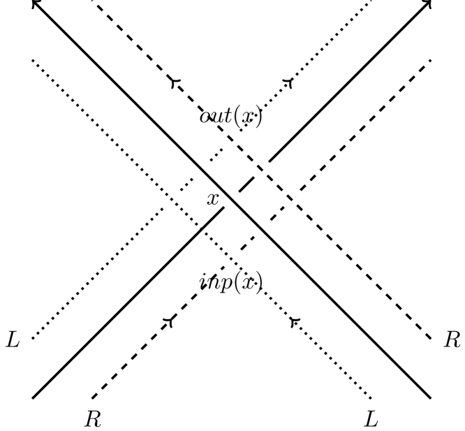
(b)

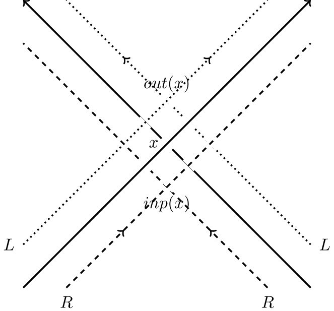
(c)

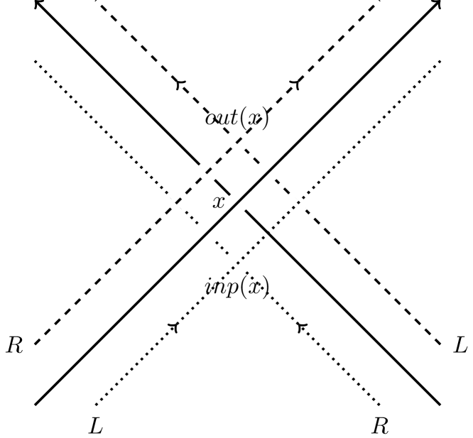
(d)

Figure 1. Segments belong to $D,{\operatorname{R}(D)}$ and ${\operatorname{L}(D)}$ are drawn by solid, dashed and dotted lines, respectively.

1.3. The sign of a crossing

Recall that in the classical situation the sign of a crossing $x$ of an oriented diagram $D$ in an oriented surface $F$ is defined to be $1$ (resp. $-1$) if the pair $(t_{1},t_{2})$ where $t_{1}$ (resp. $t_{2}$) is a positive tangent vector of overgoing (resp. undergoing) branch of $D$ at $x$, is a positive (resp. negative) basis in the tangent space of $F$ at $x$. Clearly, the definition cannot be used if the surface is non-orientable. In the following definition we use a labeled $2$-cabling of the diagram under consideration instead of the orientation of the surface in which the diagram lies.

Definition 1.

Let $D\subset\Sigma$ be a diagram of an oriented pseudo-classical knot and $D^{2}$ be a $2$-cabling of $D$. The sign of a crossing $x\in\#{D}$ is defined to be the mapping $\operatorname{sign}:\#{D}\to\mathbb{C}$ given by the following rule:

(1) $$\operatorname{sign}(x)=\begin{cases}1&\text{if ${\operatorname{R}(D)}$ goes over ${\operatorname{L}(D)}$ in ${\operatorname{inp}}(x)$ (Fig.~{}\ref{fig:1_1}),}\\ -1&\text{if ${\operatorname{L}(D)}$ goes over ${\operatorname{R}(D)}$ in ${\operatorname{inp}}(x)$ (Fig.~{}\ref{fig:1_2}),}\\ i&\text{if ${\operatorname{R}(D)}$ goes over itself in ${\operatorname{inp}}(x)$ (Fig.~{}\ref{fig:1_3}),}\\ -i&\text{if ${\operatorname{L}(D)}$ goes over itself in ${\operatorname{inp}}(x)$ (Fig.~{}\ref{fig:1_4})}\end{cases}$$

where $i\in\mathbb{C}$ is the imaginary unit.

We will say that a crossing $x\in\#{D}$ is of the type $1$ if ${\operatorname{inp}}(x)$ is an intersection of two distinct components of $D^{2}$, otherwise we will say that $x$ is of the type $2$. In other words, a crossing $x$ is of the type $1$ if $\operatorname{sign}(x)=\pm 1$ and $x$ is of the type $2$ if $\operatorname{sign}(x)=\pm i$.

Remark 1.

A crossing $x\in\#{D}$ decomposes $D$ into two closed paths $p_{1}(x),p_{2}(x)$. Both paths start at $x$ in positive direction (the first one by over-going arc, the other one by under-going arc) , then the paths go along $D$ in positive direction until the first return to $x$. Throughout we deal with pseudo-classical knots only hence, as we mentioned above, the diagram $D$ viewed as a directed path in $\Sigma$ is an orientation preserving path. Hence if $x$ is of the type $1$ then both $p_{1}(x)$ and $p_{2}(x)$ are paths preserving the orientation, while if $x$ is of the type $2$ both $p_{1}(x)$ and $p_{2}(x)$ reverses the orientation. Therefore, the situation when one of $p_{1}(x),p_{2}(x)$ preserves the orientation while the other does not is impossible in our context.

Recall that the crossing change operation in a crossing $x\in\#{D}$ is the transformation of $D$ so that overgoing arc in $x$ becomes undergoing and vice versa while the rest of the diagram remains unchanged.

The following lemma is a direct consequence of our definition of the sign and the observation that the input crossing of each $4$-crossing pattern becomes the output crossing and vice versa as a result of the reversing orientation of $D$.

Lemma 1.

(1). If a crossing $x\in\#{D}$ is of the type $1$ then each of the following transformations of $D$ and $D^{2}$ multiplies the sign of $x$ by $-1$:
a) a crossing change operation,
b) the reversing of the orientation of $D$,
c) the relabeling of $D^{2}$.

(2). If a crossing $x\in\#{D}$ is of the type $2$ then $\operatorname{sign}(x)$ is preserved under the crossing change operation while the relabeling of $D^{2}$ and the reversing orientation of $D$ multiplies the sign of $x$ by $-1$.

Remark 2.

In the classical situation when both the surface and its thickening are orientable it is natural to choose as ${\operatorname{R}(D)}$ that component of $D^{2}$ which goes to the right of $D$ with respect to its actual orientation. In the orientable case all crossings are of the type $1$ and the rule (1) gives the standard sign of a crossing. In this case the reversing orientation of the knot means in our terms simultaneous reversing orientation of $D$ and the relabeling of $D^{2}$, hence by Lemma 1(1) the signs of all crossings do not depend on the orientation of the diagram.

Having the aforementioned definition of the sign we can define an analogue of the writhe number of a diagram

$$w(D)=\sum_{x\in\#{D}}\operatorname{sign}(x)\in\mathbb{C}$$

and two more writhe numbers:

(2) $$w_{1}(D)=\sum_{\begin{subarray}{c}x\in\#{D}\\ \text{of the type }1\end{subarray}}\operatorname{sign}(x)=\operatorname{Re}w(D)\in\mathbb{R},$$

(3) $$w_{2}(D)=\sum_{\begin{subarray}{c}x\in\#{D}\\ \text{of the type }2\end{subarray}}\operatorname{sign}(x)=\operatorname{Im}w(D)\in\mathbb{R}.$$

Likewise the classical case the first Reidemeister move change the value $w(D)$, however, the following holds:

Lemma 2.

If diagrams $D_{1},D_{2}$ represent the same oriented pseudo-classical knot $K\subset\hat{\Sigma}$ then

(4) $$|w_{2}(D_{1})|=|w_{2}(D_{2})|.$$

Therefore, the absolute value of the writhe number $w_{2}$ is an isotopy invariant of a pseudo-classical knot.

Proof.

We need to consider three Reidemeister moves.

The move $R_{1}$ creates/removes a crossing of the type $1$ (Fig. 2(a)), so it does not effect the value $w_{2}$.

Both vertices involved in the move $R_{2}$ (Fig. 2(b)) are of the same type (either type $1$ or type $2$), and the reversing the orientation of $D$ and the relabeling of $D^{2}$ preserve the type. If these vertices are of the type $1$ then as in the classical case their signs are equal to $+1$ and $-1$. If the vertices are of the type  $2$ their signs are equal to $+i$ and $-i$. Hence in both cases their sum is equal to $0$ and values of all three writhe numbers ($w,w_{1},w_{2}$) are preserved under the move $R_{2}$.

The move $R_{3}$ (Figs. 2(c),2(d)) also does not effect all three writhe numbers. Therefore, all Reidemeister move do not change $w_{2}$. But we need to use the absolute value in (4) because there is no a canonical way to choose which component of $D^{2}$ is the right one, hence (see Lemma 1(2)) the value $w_{2}(D)$is defined up to multiplication by $-1$.

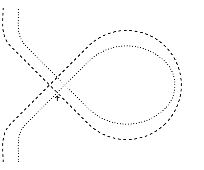
(a) The move $R_{1}$

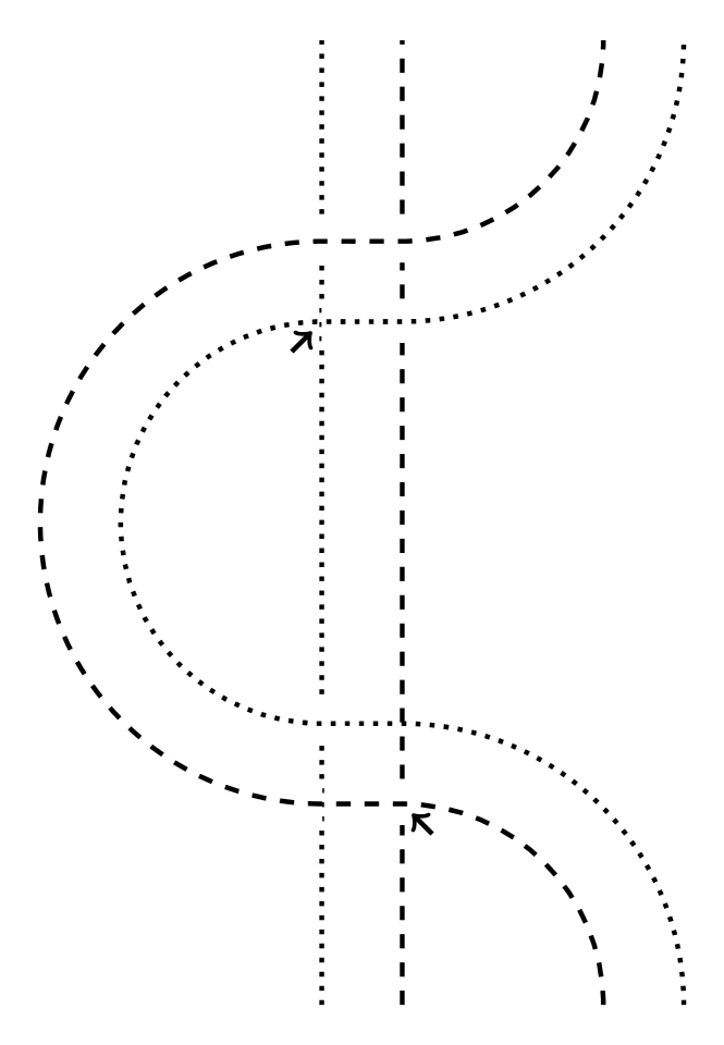
(b) The move $R_{2}$

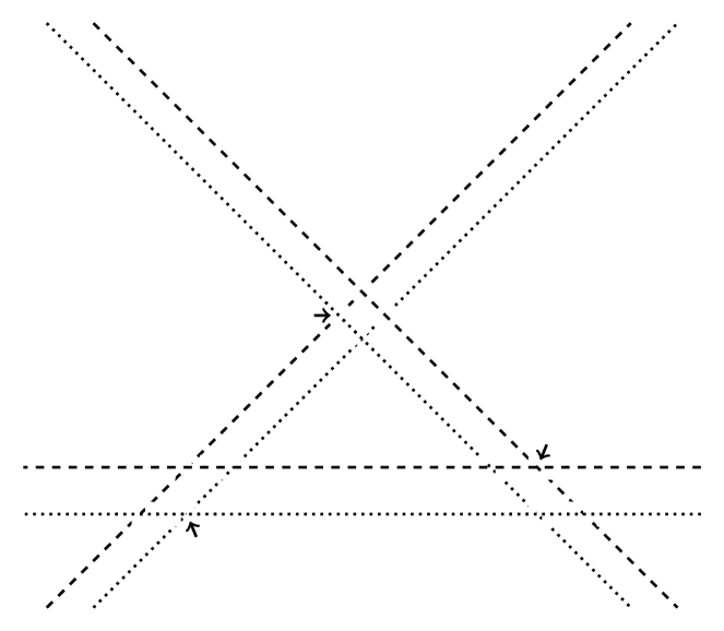
(c) Before the move $R_{3}$

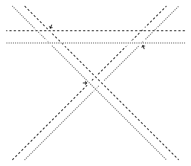
(d) After the move $R_{3}$

Figure 2. ${\operatorname{R}(D)}$ and ${\operatorname{L}(D)}$ are drawn by dashed and dotted lines, respectively. Instead of explicit specification of the orientation ${\operatorname{R}(D)}$ and ${\operatorname{L}(D)}$ we draw short arrows which point to input crossings of $4$-crossings patterns

∎

2. An analogue of the Kauffman bracket polynomial

2.1. Two types of smoothing of a crossing

To use Kauffman’s construction of the bracket polynomial [7] we need to distinguish two types of smoothing of a crossing. We will name them as positive and negative. Recall that in classical situation a smoothing of a crossing $x$ in a diagram $D$ is said to be positive if it consists in pairing of the following regions adjacent to $x$: the region lying on the right when we go to $x$ along overgoing branch of $D$ (the direction in which we go does not matter) with the region which is opposite to the first one. But, equivalently, one can define positive and negative smoothing via the sign of a crossing and the notions of smoothing along/across orientation of the diagram. Below we use the latter approach.

We begin with some auxiliary terminology. Let $D\subset\Sigma$ be a diagram representing a pseudo-classical knot. Consider a crossing $x\in\#{D}$. There is a natural correspondence between angles adjacent to $x$ and crossings forming quadrangle $4$-crossing pattern corresponding to $x$ in $D^{2}$. A smoothing of a crossing is a pairing of two vertical angles or, equivalently, a pairing of two diagonal crossings in the pattern. Hence to specify a smoothing it is sufficient to specify a pair of diagonal crossings (or even one of them only) in the pattern. We will say that a smoothing of $x$ is along the orientation of $D$ if the smoothing is determined by ${\operatorname{inp}}(x)$ (see Fig. 3(a)). The other smoothing is said to be across the orientation of the diagram (see Fig. 3(b)). Note that ${\operatorname{inp}}(x)$ and ${\operatorname{out}}(x)$ determined the same smoothing. Below in figures we will specify that type of smoothing which we want to use via short segment (which can be viewed as a diagonal of the pattern) having endpoints in that vertical angles which are pairing in the smoothing. Therefore, Figs. 3(c) and 3(d) represent smoothings of the same type as in Figs. 3(a) and 3(b), respectively.

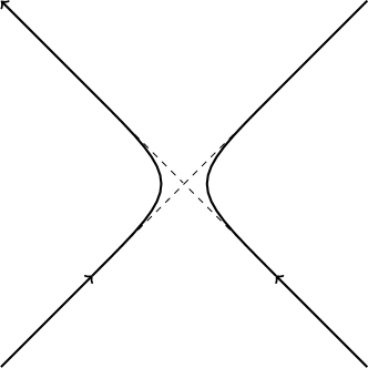
(a)

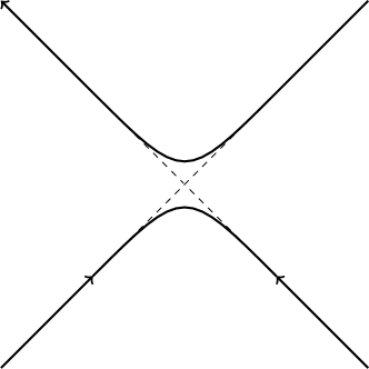
(b)

(c)

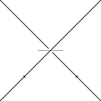
(d)

Figure 3. Smoothing along (A) and across (B) the orientation of the diagram and their simplified drawing (C) and (D), respectively.

Definition 2.

Let $D\subset\Sigma$ be an oriented diagram of an oriented pseudo-classical knot. A smoothing of a crossing $x\in\#{D}$ is called positive if it is determined by the following rule:

$$\begin{split}\text{along the orientation }&\text{ if either $\operatorname{sign}(x)=1$ or $\operatorname{sign}(x)=i$,}\\ \text{across the orientation }&\text{ if either $\operatorname{sign}(x)=-1$ or $\operatorname{sign}(x)=-i$.}\end{split}$$

Otherwise a smoothing is called negative.

Lemma 3.

Let $D\subset\Sigma$ be an oriented diagram of a pseudo-classical knot. Then for a crossing $x\in\#{D}$ the following holds:

(1). The reversing orientation of $D$ and the relabeling of $D^{2}$ make positive smoothing into negative and vice versa independently on whether $x$ is of the type $1$ or of the type $2$.

(2). The crossing change operation makes positive smoothing into negative and vice versa if $x$ is of the type $1$ and does not effect the type of smoothing otherwise.

(3). The positive smoothing in $x$ is determined by that crossing in the corresponding pattern in which overgoing arc of ${\operatorname{R}(D)}$ comes into the pattern, i.e., actual direction of the undergoing arc of $D$ and actual labeling of undergoing arcs of $D^{2}$ in the crossing do not matter which smoothing in $x$ is positive and which one is negative.

Proof.

Pick a crossing $x\in\#{D}$.

(1). By Lemma 1, both transformations (the reversing orientation of $D$ and the relabeling of $D^{2}$) multiply $\operatorname{sign}(x)$ by $-1$ independently on whether $x$ is of the type $1$ or of the type $2$. Hence, by Definition 2, these transformations make positive smoothing into negative and vice versa.

(2). This fact is again a direct consequence of Lemma 1, which states that the crossing change operation multiplies $\operatorname{sign}(x)$ by $-1$ if $x$ is of the type $1$ and preserves $\operatorname{sign}(x)$ if $x$ is of the type $2$.

(3). Denote by $y$ that crossing in which overgoing arc of ${\operatorname{R}(D)}$ comes into the pattern corresponding to $x$. There are two possibilities: either $y$ coincides with ${\operatorname{inp}}(x)$ or not. In the first case, by Definition 1, $\operatorname{sign}(x)=1$ and, by Definition 2, the positive smoothing is the one along orientation, i.e., it is determined by ${\operatorname{inp}}(x)=y$. In the second case $\operatorname{sign}(x)=-1$ and the positive smoothing is the one across orientation, i.e., it is again determined by $y$. ∎

Remark 3.

Using the third statement of the above lemma we can reformulate our definition of positive smoothing to be like the classical one: a smoothing in a crossing is positive if it is determined by that angle adjacent to the crossing which lies to the “right” when we go to the crossing along overgoing arc in positive direction. Here there are two crucial differences with the classical definition. Firstly, we have to use an ersatz-notion of the “right” constructing via a labeling of $D^{2}$ instead of the natural concept of right coming from the orientation of underlying surface. Secondly, in the classical situation the direction along which we go to the crossing does not matter while in the above definition we have to go along the positive direction if we want to use the “right” side only.

In the classical situation when both the surface and its thickening are orientable all the crossings are of the type 1 and, consequently, their signs equal $\pm 1$, and our definition of positive and negative smoothing (Definition 2) is equivalent to its classical prototype. In particular, in the classical case types of smoothing (in the sense of Definition 2) are independent on the orientation of a diagram because in the orientable situation the reversing the orientation of $D$ implies the relabeling of $D^{2}$ and, by Lemma 3(1), simultaneous performing of these two transformations preserves positive and negative smoothings.

2.2. The bracket polynomial

Below we define an analogue of the Kauffman bracket polynomial. The construction is similar to its classical prototype ([7]), the specificity of non-orientable thickening is hidden in using definitions of the sign of a crossing (Definition 1) and of positive and negative smoothing (Definition 2). The only difference is that we add a factor counting the signs of crossings of the type $2$.

Let $R$ be a ring $\mathbb{Z}[u^{\pm 1},v]$ of Laurent polynomials with integer coefficients.

Fix an oriented diagram $D$ of an oriented pseudo-classical knot $K\subset\hat{\Sigma}$.

A state of the diagram $D$ is define to be a map S: $\#{D}\to\{-1,1\}$. As usual, each state of $D$ gives rise to a collection of pairwise disjoint circles $\gamma_{1}(S),\ldots,\gamma_{n(S)}(S)\subset\Sigma$ which appear as a result of smoothings of all the crossings of $D$, type of smoothing performing in $x\in\#{D}$ is determined by the value $S(x)$: the smoothing is positive if $S(x)=1$ and negative otherwise. Let

(5) $$P(S;u)=(-u^{2}-u^{-2})^{n(S)-1}\prod_{x\in\#{D}}u^{S(x)}\in\mathbb{R}.$$

Finally set

(6) $$J(D;u,v)=(-u)^{-3w_{1}(D)}v^{|w_{2}(D)|}\sum_{S\in{\mathcal{S}}(D)}P(S;u)\in\mathbb{R}$$

where by ${\mathcal{S}}(D)$ we denote the set of all states of $D$, (for definitions of writhe numbers $w_{1}(D),w_{2}(D)$ see (2) and (3)).

Remark 4.

The value $J(D;u,v)$ depends on orientation of $D$ and actual labeling of $D^{2}$. From Lemma 3(1) and the above definition follows that the reversing of the orientation of $D$ and the relabeling of $D^{2}$ leads to substitution $u=u^{-1}$ in the polynomial $J(D;u,v)$.

Theorem 1.

If diagrams $D_{1},D_{2}\subset\Sigma$ represent the same pseudo-classical knot then either $J(D_{1},;u,v)=J(D_{2};u,v)$ or $j(D_{1};u,v)=J(D_{2};u^{-1},v)$.

Therefore, the polynomial $J(K;u,v)$ is an isotopy invariant of a pseudo-classical knot $K\subset\hat{\Sigma}$ up to substitution $u=u^{\prime-1}$.

Remark 5.

Below to make figures simpler we use the following conventions.
1. If an arc of oriented diagram $D$ is so that ${\operatorname{R}(D)}$ goes to the right of the arc the arc is drawn by solid line, otherwise when ${\operatorname{R}(D)}$ goes to the left the arc is drawn by dashed line. Here we mean the standard notion of “to the right” coming from the standard orientation of the plane of drawing.
2. Instead of explicit specifying the orientation of a diagram we draw short arrows which point to input crossings.
These conventions together with standard over/under-information allow to see both the type ($1$ or $2$) and the sign of depicted crossings (see Fig. 4).

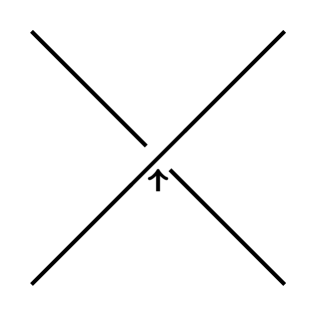
(a)

(b)

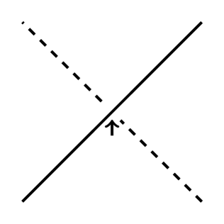
(c)

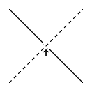
(d)

Figure 4. Depicted crossings are of the type $1$ in (a), (b) and they are of the type $2$ in (c),(d). Their signs are equal to $1,-1,i,-i$, respectively.

Proof.

The proof below is very close to the one in the classical case. The invariance of our polynomial $J$ under Reidemeister moves $R_{1}--R_{3}$ will be established by the same computations. We only need to explain why we can perform them in our case.

Fix an oriented diagram $D\subset\Sigma$ of an oriented pseudo-classical knot and a labeling of $D^{2}$.

The move ${\mathbf{R_{1}}}$. By definition of the move, a loop which the move adds/removes bounds a disk, hence (see Remark 1) a crossing which the move adds/removes is of the type $1$. and its sign is equal to $\pm 1$. There are $4$ situations depending on the value of the sign of the crossing and what passage (over or under) through the crossing we meet first going along modifying fragment. In all cases the invariance of the polynomial $J(u,v)$ under the move $R_{1}$ can be established using the same arguments as in the classical situation. However, it is necessary to remember that what of smoothing are positive is determined by what of component of $D^{2}$ is chosen as the right. For example, tangle shown in Fig. 5(a) is similar to that in the classical situation: the sign of the crossing is equal to $+1$ and positive smoothing cuts a circle. Fig. 5(b) illustrates the other case: the sign of the crossing is equal to $-1$ and the smoothing cutting a circle is negative. However, the computations proving invariance of the polynomial $J$ under the move $R_{1}$ is true for all possible situations because, by our definitions, type of smoothing and the sign of the crossing alter together. Let us, as an example, briefly consider the situation shown in Fig. 5(a). Denote by $D$ and $D^{\prime}$ the diagram before and after adding the loop, respectively. We have

$$\begin{split}J(D^{\prime};u,v)=J(D;u,v)(u+u^{-1}(-u^{2}-u^{-2}))=\\ =-J(D;u,v)u^{-3}=(-u)^{-3}J(D;u,v).\end{split}$$

Hence $J(D;u,v)=(-u)^{3}J(D^{\prime};u,v)$. The latter equality implies that the move preserves the polynomial because in this situation $w_{1}(D^{\prime})=w_{1}(D)-1$. Note that the above computation word-for-word coincides with that in the classical case when the crossing under consideration has the sign equal $-1$.

(a) $\operatorname{sign}=1$

(b) $\operatorname{sign}=-1$

Figure 5. The smoothing cutting a circle is positive in (a) and the one is negative in (b)

The move ${\mathbf{R_{2}}}$. Totally we have $16$ variants of the corresponding tangles depending on the following:
1 modifying strands are oriented in the same direction or not,
2 what of them goes over,
3 what components of $2$-cabling pass through input crossings,
4 what of these components goes over (if the two are distinct).
Both crossings which the move adds/removes are of the same type (either $1$ or $2$). In all cases one of two smoothings which cut the bigon and give an additional circle is positive while the other one is negative. Using the observation we can establish the invariance of $J(u,v)$ under the move $R_{2}$ by the same computations as in the classical situation. Again the computation coincides with that in one of $4$ situations possible in classical case. As an example, we consider variant of the move depicted in Fig. 6 which illustrates the specificity of non-orientable surface. Both crossings in Fig. 6 are of the type $2$, $\operatorname{sign}(x)=i,\operatorname{sign}(y)=-i$. To obtain an additional circle we need to perform the positive smoothing in $x$ and the negative one in $y$. Two positive and two negative smoothings gives isotopic fragments. The negative smoothing in $x$ together with positive smoothing in $y$ give a fragment isotopic to the fragment before the move. Therefore, we have

$$J(D^{\prime};u,v)=u^{-1}uJ(D;u,v)+J(D^{\prime\prime};u,v)(u^{2}+u^{-2}-u^{2}-u^{-2})=J(D;u,v)$$

where $D$ and $D^{\prime}$ — diagrams before and after the move, respectively, by $D^{\prime\prime}$ we denote that diagram which appears after performing positive smoothings both in $x$ and in $y$ in the diagram $D^{\prime}$.

Figure 6. An example of the move $R_{2}$

The move ${\mathbf{R_{3}}}$. To perform standard computation which proves the invariance of classical bracket polynomial under the move $R_{3}$ one need the following two facts. 1. The modifying tangle both before and after the transformation admits unique combination of smoothings giving an additional circle, and two of these three smoothings are positive while the third one is negative. 2. by construction an additional circle gives the additional factor $-t^{2}-t^{-2}$. Check that in our situation the same computation can be performed. Indeed, modifying tangle contains two crossings in which the same strand of the diagram $D$ goes over, and Lemma 3(3) implies that to obtain an additional circle we need to perform different smoothings in these crossings (positive in one of them and negative in the other). In the case under consideration (unlike the classical one) the third smoothing in the combination giving the circle can be both positive and negative. If it is positive the computation establishing the invariance of the polynomial $J$ word-for-word coincides with the one in classical case. The situation when the third smoothing is negative can be transform into previous one by the relabeling of $D^{2}$. The transformation changes the polynomial $J$ (see Remark 4) but the invariance of transformed polynomial under the move $R_{3}$ implies the invariance of the initial polynomial.

Finally note that, firstly, moves $R_{2}$ and $R_{3}$ does not change writhe numbers $w_{1}$ and $w_{2}$, secondly, since there is no canonical labeling of $D^{2}$ we need to use the absolute value of the writhe number $w_{2}$ and to consider the polynomial up to the substitution $u=u^{-1}$. This completes the proof of Theorem 1. ∎

Let $K\subset\hat{\Sigma}$ be a non-oriented pseudo-classical knot. In this case we define $J(K;u,v)$ as $J(K;u,v)=J(k^{\prime};u,v)$ where $K^{\prime}$ is $K$ with an arbitrary orientation. Then by Theorem 1 and Remark 4 we have the following:

Corollary 1.

The polynomial $J(K;u,v)$ is an isotopy invariant of a non-oriented pseudo-classical knot $K\subset\Sigma$ up to the substitution $U=u^{-1}$.

Remark 6.

By Lemma 3(2), the crossing change operation in a crossing of the type $2$ does not effect type of smoothing in the crossing and hence preserves the polynomial $J$. Therefore, the polynomial seems to be not very informative if diagrams under consideration has many crossings of the type $2$. The example in Section 3.1 below illustrates the fact.

2.3. A generalization of the polynomial $J$

In [3] Kauffman and Dye proposed a generalization of the Kauffman bracket polynomial for knots and links in a thickened orientable surface. The generalized polynomial takes value not in the ring of Laurent polynomial with integer coefficients but in the free module (over the latter ring) generated by the set of homology (or homotopy) classes of circles in the surface. The polynomial $J$ admits the same generalization. To this end we need to modify the monomial corresponding to each state of the diagram in question (see (5)). Namely, in the base version of the polynomial each circle in the state adds polynomial factor $-u^{2}-u^{-2}$. In the generalized version each homologically (or homotopically) trivial circle again adds to the monomial the factor $-u^{2}-u^{-2}$ while each non-trivial circle adds a factor which is the generator of the module corresponding to the homology (or homotopy) class of the circle.

3. The polynomial $J(u,v)$ vs the Kauffman bracket polynomial of double cover

Consider a non-orientable surface $\Sigma$ and a diagram $D\subset\Sigma$ of a knot $K\subset\hat{\Sigma}$. Let an orientable surface $\Sigma_{*}$ be the double cover of $\Sigma$ and $D_{*}\subset\Sigma_{*}$ denotes the diagram representing a knot (or a link) $K_{*}\subset(\Sigma_{*}\times[0,1])$ which are double covers of $D$ and $K$, respectively (here speaking of double covers of a diagram, a knot and a surface we mean mappings coming from the same double cover of the corresponding thickened surfaces). It is well-known that there is a generalization of the Kauffman bracket polynomial for knots and links in a thickened orientable surface. We denote the generalization by $J_{*}$. Clearly, $J_{*}(K_{*})$ is an invariant of $K$. In the case when $K$ is pseudo-classical we have defined above invariant $J$, and it is natural to ask whether one of these two invariants ($J$ and $J_{*}$) is a consequence of the other in particular case of pseudo-classical knots? In this section we show that the answer is “no”. More precisely, below we consider two examples, the first one (Section 3.1) when $J_{*}$ distinguishes two knots while $J$ does not, and the second one (Section 3.2) when, on the contrary, $J$ does while $J_{*}$ does not.

In both examples $\Sigma$ is the Klein bottle and $\Sigma_{*}$ is the torus. In our figures the Klein bottle is represented by a rectangle of which vertical sides are assumed to be identified via parallel translation while its horizontal sides are assumed to be identified with a twist, i.e., via the composition of parallel translation and the reflection over a vertical line. The torus is represented by a rectangle of which opposite sides (both pairs) are assumed to be identified via parallel translation.

In all cases $D_{*}$ is obtained from $D$ via the following procedure: we take two copies of a rectangle containing the diagram $D$, reflect the second copy over a vertical line and identify top side of the first copy with bottom side of the second one.

Before considering examples we need to make a remark on the construction of the Kauffman bracket polynomial. It is well-known that in classical situation one can define the Kauffman bracket polynomial for non-oriented knots, at the same time, in the case of links orientations of components matter. The reason is that the factor which makes the polynomial invariant under the first Reidemeister move depends on the writhe number of the diagram under consideration, while the signs of intersection points of distinct components have sense for oriented links only. To make the Kauffman bracket polynomial into an invariant of non-oriented links it is sufficient to ignore intersections of distinct components when we compute the factor. But usually the signs of these crossings are taken into account in the construction of the polynomial and below we follow the tradition. However, in all cases below diagrams which are double cover by construction (the union of a diagram with its mirror reflection) have writhe number equals zero hence both approaches to the definition of the Kauffman bracket polynomial (including and excluding the signs of intersection points of distinct components) lead to polynomials having coinciding values on the diagrams in question.

3.1. An example when $J_{*}$ is stronger than $J$

Consider two diagrams in the Klein bottle: $D_{1}$ (Fig. 7(a)) and $D_{2}$ (Fig. 7(b)). Each of these diagrams has two intersections with horizontal side of the rectangle representing the Klein bottle (recall horizontal sides assume to be identify with a twist) hence knots represented by these diagrams are pseudo-classical, and the polynomial $J$ has sense for both of them.

Note that $D_{1}$ can be obtained from $D_{2}$ as a result of two transformations: the crossing change operation in the crossing $u$ and then the second Reidemeister move removing $u$ and $v$.

Components of $2$-cabling of a diagram on the Klein bottle permute when the diagram passes through horizontal sides of depicted rectangle hence the diagram $D_{2}$ has $3$ crossings (including $u$ and $v$) of the type $2$. As we mentioned above in Remark 6 the crossing change operation in a crossing of the type $2$ preserves the polynomial $J$. The second Reidemeister move preserves $J$ also. Therefore, both transformations which make $D_{2}$ into $D_{1}$ preserve the polynomial $J$, thus $J(D_{1})=J(D_{2})$.

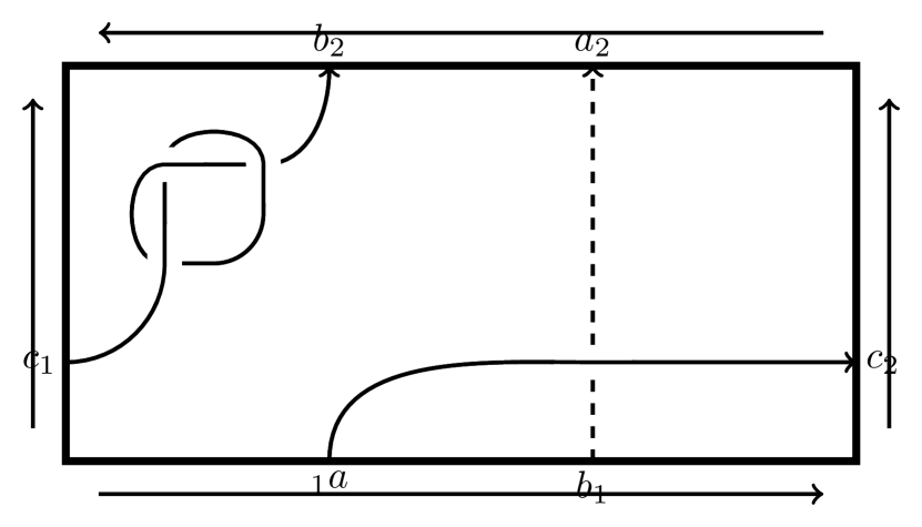
(a) $D_{1}$

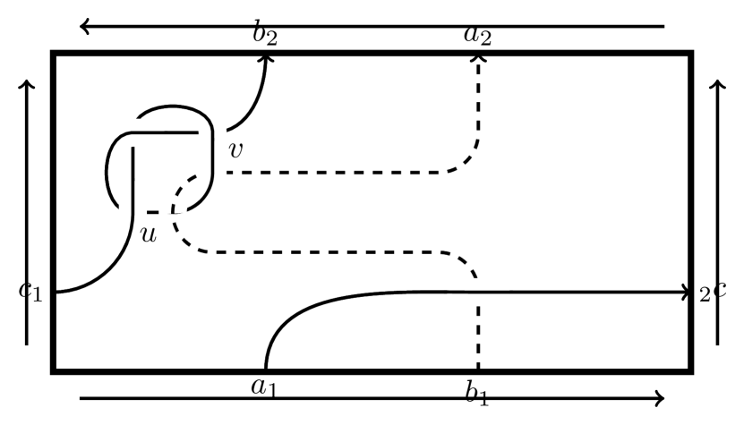
(b) $D_{2}$

Figure 7. Diagrams in the Klein bottle

Diagrams $D_{1*}$ (Fig. 8(a)) and $D_{2*}$ (Fig. 8(b)) in the torus are double covers of $D_{1}$ and $D_{2}$, respectively. $D_{1*}$ has $8$ crossings, $D_{2*}$ has $12$ crossings, so the computation of $J_{*}(D_{1*})$ and, especially, $J_{*}(D_{2*})$ is too cumbersome to be made by hand. The values below are computed by “3–manifold recognizer” [4] — a computer program for studying $3$–manifolds and knots.

$$\begin{split}J_{*}(D_{1*})&=t^{-14}-2t^{-2}-2t^{2}+t^{14},\\ J_{*}(D_{2*})&=t^{-18}-t^{-14}+t^{-10}-t^{-6}-t^{-2}-t^{2}-t^{6}+t^{10}-t^{14}+t^{18}.\end{split}$$

(In Appendix below we give source data needed for computing the values above in the format acceptable by the program “3–manifold recognizer”.) We see that these two polynomials are distinct.

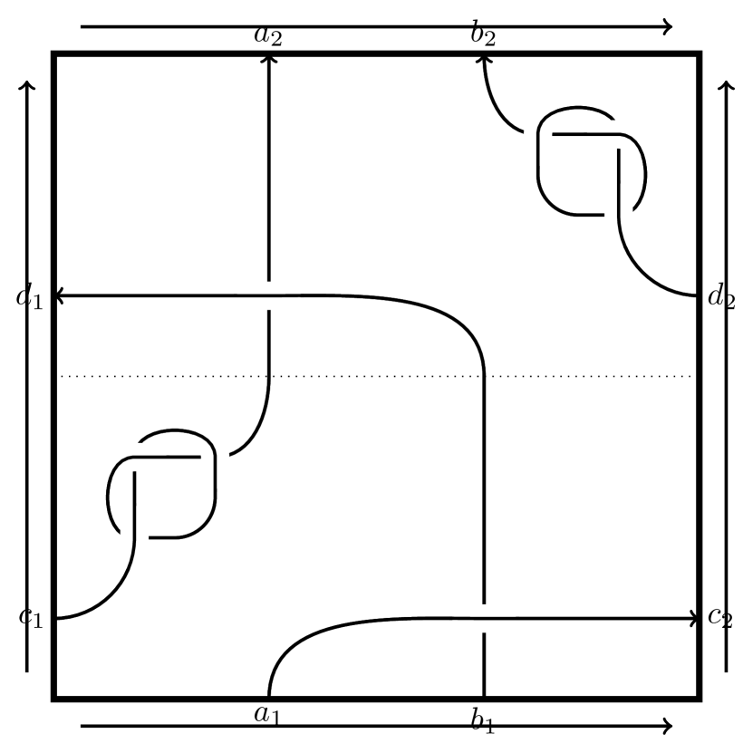
(a) $D_{1*}$

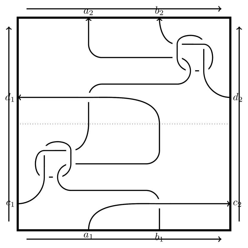
(b) $D_{2*}$

Figure 8. Diagrams in the torus which are the double cover of $D_{1}$ and $D_{2}$, respectively

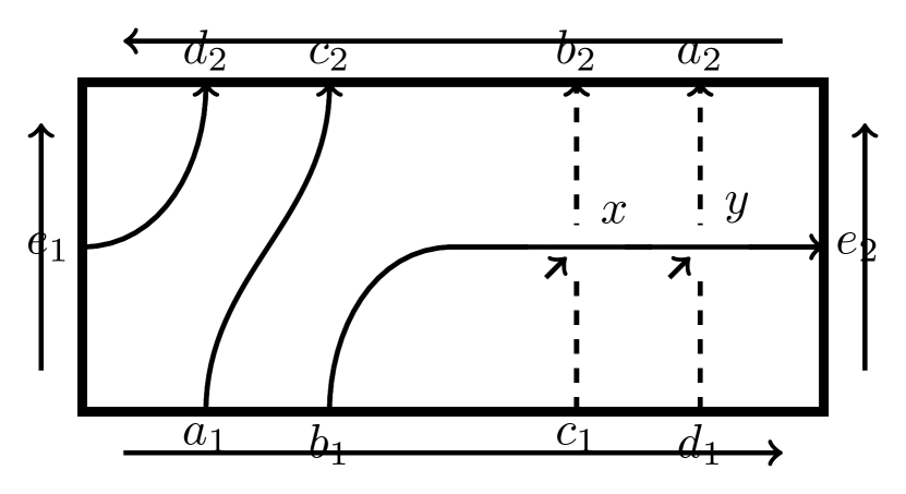
(a) $D_{3}$

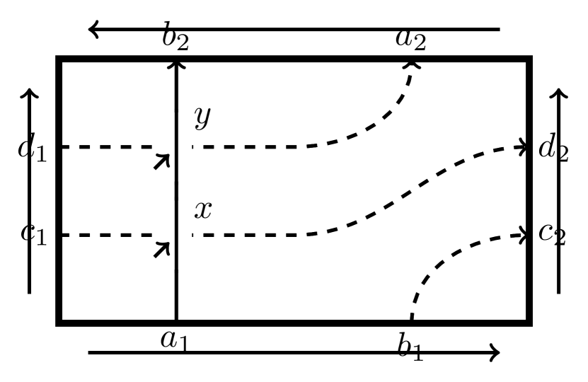
(b) $D_{4}$

Figure 9. Diagrams in the Klein bottle so that $J(D_{3})\neq J(D_{4})$.

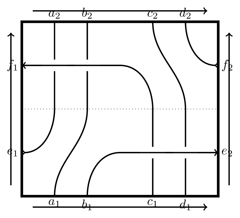
(a) $D_{3*}$

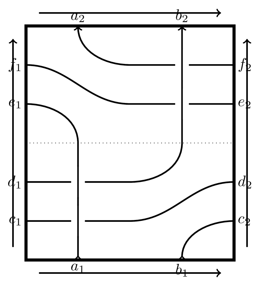
(b) $D_{4*}$

Figure 10. Diagrams in the torus which are the double cover of $D_{3}$ and $D_{4}$, respectively. $D_{4*}$ obtains (up to orientation of components) from $D_{3*}$ by rotation by $90^{\circ}$ in the clockwise direction.

3.2. An example when $J$ is stronger than $J_{*}$

The diagrams $D_{3}$ (Fig. 9(a)) and $D_{4}$ (Fig. 9(b)) in the Klein bottle so that $J(D_{3})\not=J(D_{4})$ (the fact will be established below). At the same time, the diagrams $D_{4*}$ (Fig. 10(a)) and $D_{4*}$ (Fig. 10(b)) in the torus which are double covers of $D_{3}$ and $D_{4}$, respectively, represents $2$-component links in the thickened torus which have coinciding values of $J_{*}$. To establish the equality $J_{*}(D_{3*})=J_{*}(D_{4*})$ it is sufficient to observe that $D_{4*}$ obtains from $D_{3*}$ as a result of the rotation by $90^{\circ}$ in the clockwise direction and the reversing the orientation of that component which in Fig. 10(a) passes through points $a_{1}=a_{2},b_{1}=b_{2},c_{1}=c_{2}$. The fact implies the required equality because, as we mentioned in the beginning of Section 3, value of the polynomial $J_{*}$ does not depend on the orientation of link components in the case under consideration. One can show that links in the thickened torus represented by $D_{3*}$ and $D_{4*}$ are inequivalent as oriented links but it is not necessary in our context.

Now we compute $J(D_{3})$ and $J(D_{4})$.

3.2.1. Computation of $J(D_{3})$

The diagram $D_{3}$ (Fig. 9(a)) has $2$ crossings denoted by $x$ and $y$ hence to compute $J(D_{3})$ we need to consider $4$ states $S_{1},\ldots,S_{4}$ of the diagram which map the pair of its crossings $(x,y)$, respectively, to the pairs $(1,1)$, $(1,-1)$, $(-1,1)$, $(-1,-1)$. Below circles which appear as a result of smoothings $n(S_{j})$ (for shortness the parameter $S_{j}$ will be omitted) are presented as the union of arcs having endpoints in the sides of depicted rectangle. For the definition of polynomial $P(S;u)$ corresponding to each state of a diagram see (5).

$S_{1}$: $(1,1)$ $n(S_{1})=3$,
$\gamma_{1}=[a_{1},c_{2}]\cup[c_{1},a_{2}]$, $\gamma_{2}=[b_{1},b_{2}]$, $\gamma_{3}=[d_{1},e_{2}]\cup[e_{1},d_{2}]$,
$P(S_{1};u)=u^{2}(-u^{2}-u^{-2})^{2}=u^{6}+2u^{2}+u^{-2}$;

$S_{2}$: $(1,-1)$ $n(S_{2})=2$,
$\gamma_{1}=[a_{1},c_{2}]\cup[c_{1},d_{1}]\cup[d_{2},e_{1}]\cup[e_{2},a_{2}]$, $\gamma_{2}=[b_{1},b_{2}]$,
$P(S_{2};u)=u\,u^{-1}(-u^{2}-u^{-2})=-u^{2}-u^{-2}$;

$S_{3}$: $(-1,1)$ $n(S_{3})=2$,
$\gamma_{1}=[a_{1},c_{2}]\cup[c_{1},b_{1}]\cup[b_{2},a_{2}]$, $\gamma_{2}=[d_{1},e_{2}]\cup[e_{1},d_{2}]$,
$P(S_{3};u)=u^{-1}u(-u^{2}-u^{-2})=-u^{2}-u^{-2}$;

$S_{4}$: $(-1,-1)$ $n(S_{4})=1$,
$\gamma_{1}=[a_{1},c_{2}]\cup[c_{1},b_{1}]\cup[b_{2},d_{1}]\cup[d_{2},e_{1}]\cup[e_{2},a_{2}]$,
$P(S_{4};u)=u^{-2}$.

To compute the resulting value of $J(D_{3})$ we need to know values of writhe numbers $w_{1}$ (see (2)) and $w_{2}$ (see (3)). The diagram $D_{3}$ has $2$ crossings, both are of the type $2$, hence $w_{1}(D_{3})=0$. Both input crossings ${\operatorname{inp}}(x)$ and ${\operatorname{inp}}(y)$ are self-intersection of ${\operatorname{R}(D_{3})}$ thus $\operatorname{sign}(x)=\operatorname{sign}(y)=i$ thus $w_{2}(D_{3})=2$.

Therefore (see (6)),
$J(D_{3};u,v)=u^{0}v^{2}\sum P(S_{j},u)=v^{2}(u^{6}+2u^{2}+u^{-2}-u^{2}-u^{-2}-u^{2}-u^{-2}+u^{-2})=u^{6}v^{2}$.

3.2.2. Computation of $J(D_{4})$

The diagram $D_{4}$ (Fig. 9(b)) has $2$ crossings denoted by $x$ and $y$ hence to compute $J(D_{4})$ we again need to consider $4$ states of the diagram.

$S_{1}$: $(1,1)$ $n(S_{1})=1$,
$\gamma_{1}=[a_{1},f_{2}]\cup[f_{1},b_{2}]\cup[b_{1},e_{2}]\cup[e_{1},a_{2}]$,
$P(S_{1};u)=u^{2}$;

$S_{2}$: $(1,-1)$ $n(S_{2})=1$,
$\gamma_{1}=[a_{1},f_{2}]\cup[f_{1},e_{1}]\cup[e_{2},b_{1}]\cup[b_{2},a_{2}]$,
$P(S_{2};u)=u\,u^{-1}=1$;

$S_{3}$: $(-1,1)$ $n(S_{3})=1$,
$\gamma_{1}=[a_{1},e_{1}]\cup[e_{2},b_{1}]\cup[b_{2},f_{1}]\cup[f_{2},a_{2}]$,
$P(S_{3};u)=u^{-1}u=1$;

$S_{4}$: $(-1,-1)$ $n(S_{4})=2$,
$\gamma_{1}=[a_{1},e_{1}]\cup[e_{2},b_{1}]\cup[b_{2},a_{2}]$, $\gamma_{2}=[f_{1},f_{2}]$,
$P(S_{4};u)=u^{-2}(-u^{2}-u^{-2})=-1-u^{-4}$.

The writhe numbers have the same values as above, hence
$J(D_{4};u,v)=v^{2}(u^{2}+1+1-1-u^{-4})=v^{2}(u^{2}+1-u^{-4})$.

Therefore, $J(D_{3})\not=J(D_{4})$ and the substitution $u=u^{-1}$ does not transform one of them into another thus by Theorem 1 knots in (the Klein bottle) $\times[0,1]$ represented by these diagrams are inequivalent.

Appendix: Source data for a computation via the computer program “3–manifold recognizer”

To compute the Kauffman bracket polynomial of a knot (or a link) in the thickened torus via the computer program “3–manifold recognizer” [4] it is necessary to describe the knot (or link) in question using an extended Gauss code. Namely, we begin with numbering of the crossings of the diagram by natural numbers from $1$ in increasing order. The crossings of the diagram with sides of the rectangle in which the diagram lies are denoted by a letter and a number which follows the letter without space between them. Letters $l,t,r,b$ mean that the corresponding crossing lies on left, top, right, bottom side of the rectangle, respectively. The number is the number of the crossing in corresponding side. For all $4$ sides these numbers increase in the clockwise direction. For example, l1 denotes the lowermost intersection with the left side while r1 denotes the topmost intersection with the right one, t1 denotes the leftmost intersection with the top side while b1 denotes the rightmost intersection with the bottom one. The meaning of all other lines in the following description of the links seems to be clear.

The description of the diagram $\mathbf{D_{1}*}$. (Fig 8(a))

link  T^2
crossings 8
signs 1 1 1 1 -1 -1 -1 -1
code 1 -2 3 -1 2 -3 -8 t1 b2 4 r2 l1
code -4 8 l2 r1 5 -6 7 -5 6 -7 t2 b1
end
 

The description of the diagram $\mathbf{D_{2}*}$. (Fig 8(b))

link  T^2
crossings 12
signs 1 1 1 1 -1 -1 -1 -1 1 1 -1 -1
code 1 -2 3 9 -10 -1 2 -3 -8 12 -11 t1 b2 4 r2 l1
code -4 10 -9 8 l2 r1 5 -6 7 11 -12 -5 6 -7 t2 b1
end

References

- [1] Mario O. Bourgoin. Twisted link theory. Algebr. Geom. Topol., 8(3):1249–1279, 2008.
- [2] Yu. V. Drobotukhina. An analogue of the Jones polynomial for links in and a generalization of the Kauffman-Murasugi theorem. Algebra i Analiz, 2(3):171–191, 1990.
- [3] H. A. Dye and Louis H. Kauffman. Minimal surface representations of virtual knots and links. Algebr. Geom. Topol., 5:509–535, 2005.
- [4] Evgeny Fominykh, Sergei Matveev, and Vladimir Tarkaev. 3-manifold recognizer, a computer program for studying of 3-manifolds and knots. Available at http://matlas.math.csu.ru (19/09/2022).
- [5] Allison Henrich. A sequence of degree one Vassiliev invariants for virtual knots. J. Knot Theory Ramifications, 19(4):461–487, 2010.
- [6] Naoko Kamada and Seiichi Kamada. Double coverings of twisted links. J. Knot Theory Ramifications, 25(9):1641011, 22, 2016.
- [7] Louis H. Kauffman. State models and the Jones polynomial. Topology, 26(3):395–407, 1987.
- [8] Louis H. Kauffman. Virtual knot theory. European J. Combin., 20(7):663–690, 1999.
- [9] Louis H. Kauffman. An affine index polynomial invariant of virtual knots. J. Knot Theory Ramifications, 22(4):1340007, 30, 2013.
- [10] Kirandeep Kaur, Madeti Prabhakar, and Andrei Vesnin. Two-variable polynomial invariants of virtual knots arising from flat virtual invariants. J. Knot Theory Ramifications, 27(13):1842015, 22, 2018.
- [11] S. V. Matveev and L. R. Nabeeva. Tabulation of knots in a thickened Klein bottle. Sibirsk. Mat. Zh., 57(3):688–696, 2016.
- [12] Vladimir Tarkaev. Homological invariants of links in a thickened surface. Rev. R. Acad. Cienc. Exactas F??s. Nat. Ser. A Mat. RACSAM, 1141):Paper No. 17, 19, 2020.
- [13] V. A. Vassiliev. On invariants and homology of spaces of knots in arbitrary manifolds. In Topics in quantum groups and finite-type invariants, volume 185 of Amer. Math. Soc. Transl. Ser. 2, pages 155–182. Amer. Math. Soc., Providence, RI, 1998.
- [14] Victor A. Vassiliev. Linking numbers in non-orientable 3-manifolds. J. Knot Theory Ramifications, 25(12):1642016, 13, 2016.