Large-Scale Allocation of Personalized Incentives

Abstract

We consider a regulator willing to drive individual choices towards increasing social welfare by providing incentives to a large population of individuals.

For that purpose, we formalize and solve the problem of finding an optimal personalized-incentive policy: optimal in the sense that it maximizes social welfare under an incentive budget constraint, personalized in the sense that the incentives proposed depend on the alternatives available to each individual, as well as her preferences. We propose a polynomial time approximation algorithm that computes a policy within few seconds and we analytically prove that it is boundedly close to the optimum. We then extend the problem to efficiently calculate the Maximum Social Welfare Curve, which gives the maximum social welfare achievable for a range of incentive budgets (not just one value). This curve is a valuable practical tool for the regulator to determine the right incentive budget to invest.

Finally, we simulate a large-scale application to mode choice in a French department (about 200 thousands individuals) and illustrate the effectiveness of the proposed personalized-incentive policy in reducing CO₂ emissions.

I Introduction

Taxes and subsidies in transportation are often perceived by the population as unfair, since they neglect the alternatives actually available to each individual and the individual preferences. On the other hand, with the increase in information available to governments [1], economic policies can be improved to consider the peculiarities of each individual. We propose a policy of personalized incentives in a framework where individuals choose between multiple alternatives options. A regulator has a limited budget that he can use to propose monetary incentives, with the goal to induce individuals to change their choice toward socially-better ones. Most incentive policies in the literature are not personalized [2, 3], with some exception [4]. Differently from the latter, we seek for a method with provable performance bounds.

We define the optimal personalized-incentive policy as the allocation of incentives that maximizes social welfare (defined as the reduction of CO₂ emissions in the example above), for a given budget. We formalize the problem of finding a personalized-incentive policy maximizing social welfare under the regulator’s budget constraint and show that it reduces to the well-known Multiple-Choice Knapsack Problem (MCKP – §II), which has been used in several contexts, like Economics [5] and Computer Science [6]. To approximate the optimal policy in polynomial time, we adapt a greedy algorithm from the Operations Research literature and we analyze some of its analytical (e.g., suboptimality gap bound) and economic (e.g., diminishing returns) properties (§III). While in most of the paper we assume that the regulator knows exactly the preferences of each individual, we also study the case of imperfect information (§IV).

Using data from the French census at the scale of a French department, we evaluate the CO₂ reduction achieved via the transportation mode incentive policy computed with our algorithm (§ V). The results show that our personalized incentives achieve the same CO₂ reduction as flat subsidies, but with a considerably smaller amount of incentives spent. Our code is available as open source [7].

We are aware that our framework is based on several idealized assumptions that makes its direct applicability difficult in practical situations, in particular for what concerns the assumption of being able to collect precise information about individual preferences. In this sense, the path toward personalized-incentives is still a long way to go. However, we argue that the theoretical findings of this paper, coupled with the continuous evolution of techniques for collecting societal big-data, while respecting privacy, provide important steps along this path.

II Framework and Incentive Policy

II-A Model

We consider a population $\mathcal{I}\equiv\{1,\dots,m\}$ of $m$ individuals. Each individual $i\in\mathcal{I}$ chooses an alternative $j$ among an individual-specific choice-set $\mathcal{N}_{i}$. For example, we can consider individuals choosing a mode of transportation to commute to their work. In this case, the choice set could be $\mathcal{N}_{i}=\{\text{car},\text{walk},\text{bike},\text{public transit}\}$. The choice set can be individual-specific so that if individual $i$ owns a car but individual $i^{\prime}$ does not, we could have $\mathcal{N}_{i}=\{\text{car},\text{walk},\text{bike},\text{public transit}\}$ and $\mathcal{N}_{i^{\prime}}=\{\text{walk},\text{bike},\text{public transit}\}$.

Let $y_{i,j}>0$ be an incentive provided by the regulator to individual $i$, when she chooses alternative $j$. Since $y_{i,j}$ changes from an individual to another, such policy is personalized.

A policy influences the individual choice since the proposed monetary transfers change her utilities. The utility $U_{i,j}$ of individual $i$ when choosing alternative $j\in\mathcal{N}_{i}$ is given by $U_{i,j}=V_{i,j}+y_{i,j},$, where $V_{i,j}\in\mathbb{R}$ is the intrinsic utility (in the absence of policy). Each individual $i$ chooses an alternative $j^{*}_{i}$ which maximizes her utility $j^{*}_{i}\in\operatorname*{arg\,max}_{j}U_{i,j}.$ Each alternative $j$ of individual $i$ is characterized by a social indicator $b_{i,j}\in\mathbb{R}$ (e.g., the opposite of CO₂ emissions induced by the commutes).

We assume the regulator has perfect information: it knows exactly the intrinsic utilities $\{V_{i,j}\}_{i,j}$ and social indicators $\{b_{i,j}\}_{i,j}$ of all the alternatives, for all the individuals. We will relax this assumption in §IV.

The alternative chosen by each individual $i$ in the absence of policy (i.e., where $y_{i,j}=0$, $\forall i,j$) is called default alternative, and denoted $j^{0}_{i}\triangleq\operatorname*{arg\,max}_{{j^{\prime}}\in\operatorname*{arg\,max}_{j}V_{i,j}}b_{i,{j^{\prime}}}$. In order to convince an individual $i$ to shift from its default alternative to any other alternative $j$, it is necessary and sufficient for the regulator to provide an incentive $w_{i,j}\triangleq V_{i,j^{0}_{i}}-V_{i,j}$, to compensation for the decrease of individual utility.

II-B Maximum Social Welfare Problem

The regulator has to decide, for each individual $i$, which alternative to incentivize, which can be summarized by a binary decision variable $x_{i,j}$ that is equal to $1$ if the regulator wants to make individual $i$ choose alternative $j$, and $0$ otherwise. The incentive can be thus written as $y_{i,j}=x_{i,j}\cdot w_{i,j}$. The Maximum Social Welfare problem is

$$\max_{\{x_{i,j}\}_{i,j}} \sum_{i\in\mathcal{I}}\sum_{j\in\mathcal{N}_{i}}b_{i,j}x_{i,j}$$ (1)

s.t. $$\sum_{i\in\mathcal{I}}\sum_{j\in\mathcal{N}_{i}}w_{i,j}x_{i,j}\leq Q$$ (2)

$$\sum_{j\in\mathcal{N}_{i}}x_{i,j}=1, i\in\mathcal{I}$$ (3)

$$x_{i,j}\in\{0,1\}, i\in\mathcal{I},\ j\in\mathcal{N}_{i}$$ (4)

The objective function (1) aims to maximize the social welfare, i.e., the sum of all social indicators, constraint (2) indicates that the regulator cannot spend more than $Q$. Moreover, only one alternative per individual is incentivized (3).

For any budget $Q$, we indicate with $B^{*}(Q)$ the maximum of the social welfare, solution of problem (1).

II-C Maximum Social Welfare Curve Problem

Suppose now that the regulator is endowed with a maximum budget $Q$ and that he can spend any budget in the interval $Y\in[0,Q]$. To decide the exact amount of budget that is convenient to spend, it is useful to obtain the Maximum Social Welfare Curve $\mathcal{C}^{*}_{Q}$, representing the maximum social welfare reachable, $B^{*}(Y)$, for any budget $Y\in[0,Q]$, i.e. $\mathcal{C}^{*}_{Q}=\left\{\big{(}Y,B^{*}(Y)\big{)}\>\middle|\>Y\in[0,Q]\right\}$, which is clearly monotone non-decreasing (the larger the budget spent, the larger the social welfare reached). Observe that, although a maximum budget $Q$ is available, the regulator may not want to indiscriminately spend it all, but may choose the actual budget to invest in incentives, based on several criteria. For instance, the regulator may use the above curve to find the minimum budget needed to reach a certain social-welfare target (see the example of Fig. 3).

III Approximation Algorithm

The MCKP problem, and thus the Maximum Social Welfare problem (1), is NP-hard [8] . We provide in this section a polynomial time algorithm based on greedy algorithms from the Operations Research literature, which gives us solutions boundedly close to the optimum.

III-A Preliminary Steps

Before presenting the proposed algorithm, we need to “clean” the input of the problem, removing some irrelevant alternatives from the set $\mathcal{N}_{i}$ of the alternatives of any individual $i$ [8, Section 11.2.1]. In broad terms, irrelevant alternatives are the ones that do not provide enough social indicator compared to the incentive amount needed to induce them. The alternatives remaining after the cleaning are usually called LP-extremes and we denote them with $\mathcal{R}_{i}\subseteq\mathcal{N}_{i}$. Figure 1 gives the intuition behind the process of constructing the set $\mathcal{R}_{i}$, which is called concavization [9, Fig.1,2]. In the figure, alternative $3$ is irrelevant since $2$ provides a larger social indicator, while requiring less incentive. Alternative $7$ is irrelevant since it requires to spend more incentive than $6$, for a negligible gain in the social indicator. It is much more convenient to make a slightly bigger investment to induce alternative $9$, which provides a significant social indicator improvement with respect to $6$.

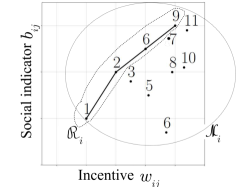
Figure 1: Alternative set $\mathcal{N}_{i}$ of individual $i$ and the subset $\mathcal{R}_{i}$ of LP-extremes.

We follow the Operations Research literature in the slight abuse of notation of denoting with $w_{i,j}$ the incentive to be provided to the $j$-th alternative in $\mathcal{R}_{i}$. With no loss of generality, we can assume the ordering $w_{i,1}<w_{i,2}<\dots<w_{i,|\mathcal{R}_{i}|}$. Obviously, the default alternative is the first alternative in the set $\mathcal{R}_{i}$ and $w_{i,1}=0$.

Definition III-A.1 (Efficiency and incremental efficiency).

We define the efficiency of an alternative $j$ of individual $i$ as $e_{i,j}\triangleq\frac{b_{i,j}-b_{i,j^{0}_{i}}}{w_{i,j}}$, i.e., the gain in social indicator that we can gain via a unit of incentive allocated to that alternative.

We also define the incremental social indicator $\tilde{b}_{i,j}$ and the incremental incentive $\tilde{w}_{i,j}$ required for each alternative $j\in\mathcal{R}_{i}$ as

$$\begin{array}[]{rl}\tilde{b}_{i,j}&\triangleq b_{i,j}-b_{i,j-1}\\ \tilde{w}_{i,j}&\triangleq w_{i,j}-w_{i,j-1}\end{array},\quad j=2,\dots,|\mathcal{R}_{i}|.$$ (5)

The incremental efficiency is then defined as $\tilde{e}_{i,j}\triangleq\tilde{b}_{i,j}/\tilde{w}_{i,j}.$

The incremental efficiency $\tilde{e}_{i,j}$ can be interpreted as the increase in social welfare for each monetary unit spent, when individual $i$ shifts from alternative $j-1$ to alternative $j$.

III-B Greedy Algorithm

Very efficient algorithms [8, Section 11.2.1] are known to solve problem (1), i.e., to approximate the maximum social welfare for a fixed single value of budget $Q$. However, to apply them to the Maximum Social Welfare Curve problem, in which we want to find the maximum social welfare for a range of budget values $Y\in[0,Q]$, instead of just one, we would have to run those algorithms from scratch for every single value of budget. For this reason, we build our solutions upon a simpler greedy algorithm [8, Figure 11.2], which is less efficient to solve the Maximum Social Welfare problem (although still polynomial in time complexity), but easily extendable to also solve the Maximum Social Welfare Curve problem. The other advantage deriving from such choice is that this greedy algorithm has interesting properties that increase its practical application.

The pseudocode of the algorithm is in Algorithm 1. The notation $[i,j]$ stands for “$j$-th alternative of individual $i$”. First, the algorithm finds all the LP-extremes alternatives and sort them by order of decreasing incremental efficiency. Then, at each iteration, the next pair $[i^{\prime},j^{\prime}]$ with the highest incremental efficiency is picked (line 1). The alternative induced to $i^{\prime}$ is set to $j^{\prime}$ (line 1) and the budget is reduced by the amount of the incremental weight (6). An additional piece of the approximation of the social welfare curve is computed (8). The algorithm stops when the maximum budget $Q$ is depleted.

Input : Social indicators $\{b_{i,j}\}_{i,j}$, intrinsic utilities $\{V_{i,j}\}_{i,j}$, budget $Q$

1 Iteration index $k:=0$

2 $Y^{[k]}:=0$, Total incentive allocated so far.

3 ${B}^{[k]}:=0$, Social welfare obtained in the current allocation.

4 Compute the ordered set $\mathcal{R}_{i}$ of LP-extremes of each individual $i$.

5 Sort all the alternatives $[i,j]$ according to decreasing incremental efficiency $\tilde{e}_{i,j}$ and put them in a set $\mathcal{R}$.

6 Initialize the alternatives chosen by the individuals $\{x_{i,j}\}_{i,j}$ as follows

$$\left\{\begin{array}[]{ll}x_{i,1}=1,&\text{(default alternative)}\\ x_{i,j}=0,&\text{for any alternative }j>1\end{array}\right.$$

7 while $\mathcal{R}\neq\emptyset$ and $Y^{[k]}\leq Q$ do

8       Take $[i^{\prime},j^{\prime}]$, the next alternative with the highest incremental efficiency $\tilde{e}_{i^{\prime},j^{\prime}}$ from $\mathcal{R}$.

9       Add $[i^{\prime},j^{\prime}]$ to the solution, i.e.:

$$\mathcal{R} :=\mathcal{R}\setminus\{[i^{\prime},j^{\prime}]\},$$

$$Y^{[k+1]} :=Y^{[k]}+\tilde{w}_{i^{\prime},j^{\prime}}$$ (6)

$$\tilde{e}^{[k]} :=\tilde{e}_{i^{\prime},j^{\prime}}$$ (7)

$$B(Y) :={B}^{[k]}, \forall Y\in[Y^{[k]},Y^{[k+1]})$$ (8)

$${B}^{[k+1]} :={B}^{[k]}+\tilde{b}_{i^{\prime},j^{\prime}}$$

$$k :=k+1$$

10       Update the selected alternative for individual $i^{\prime}$, i.e.,

$$\left\{\begin{array}[]{rll}x_{i^{\prime},j^{\prime}}&=1,&\\ x_{i^{\prime},j}&=0,&\text{ for any other alternative }j\neq j^{\prime}\end{array}\right.$$

Output :  Curve $\mathcal{C}_{Q}=\left\{(Y,B(Y))\>|\>Y\in[0,Q]\right\}$

Chosen alternatives $\{x_{i,j}\}_{i,j}$

Incentive policy $\mathbf{y}=\{y_{i,j}\}_{i,j}$, where $y_{i,j}=x_{i,j}\cdot w_{i,j}$

Split item $[s,t]:=[i^{\prime},j^{\prime}]$

Incremental efficiency of the split item $\tilde{e}_{s,t}$

Budget actually used $\tilde{Q}:=Y^{[k-1]}$

Algorithm 1 Greedy algorithm for the Maximum Social Welfare and Maximum Social Welfare Curve problems.

Observe that the curve $\mathcal{C}_{Q}$ given as output by the algorithm is an approximation of the solution $\mathcal{C}^{*}_{Q}$ of the Maximum Social Welfare Curve Problem (Section II-C). Moreover, given any maximum budget $Q$, the algorithm returns an approximation $B(Q)$ to the solution $B^{*}(Q)$ of the Maximum Social Welfare Problem (1). Note that, in order to achieve $B(Q)$, the policy issued by the algorithm does not spend the entire maximum budget $Q$, but only $\tilde{Q}\leq Q$.

The algorithm also gives as output the incremental efficiency of the “split item”, denoted with $\tilde{e}_{s,t}$, useful to compute the optimality gap of the algorithm (Theorem III-B.1 below). The name split item, which we borrow from [8], reminds that, when we allocate budget $Q$, we add to the solution all the LP-extreme alternatives, in decreasing order of incremental efficiency, up to the “split alternative” $[s,t]$, as $[s,t]$ actually splits the set $\mathcal{R}$ of all LP-extremes in two subsets: the first containing the alternatives to include in our solution, while we do not include the LP-extremes from the second subset.

The following statements guarantee that the result from the algorithm is boundedly close to the optimum. We omit the proofs for lack of space, which can be obtained by adapting [8, Ch.11].

Theorem III-B.1 (Upper bound).

Let us run Alg. 1 with budget $Q$, and let $\tilde{Q}$ be the budget actually used and $\tilde{e}_{s,t}$ be the incremental efficiency of the split item. The social welfare $B(Q)$ we obtain is boundedly close to the social welfare $B^{*}(Q)$ of any optimal personalized-incentive policy:

$$B^{*}(Q)-B(Q)\leq\tilde{e}_{s,t}\cdot(Q-\tilde{Q}).$$ (9)

Corollary III-B.2.

The curve $\mathcal{C}_{Q}$ obtained via Algorithm 1 is boundedly close to the Maximum Social Welfare Curve $\mathcal{C}^{*}_{Q}$ from (II-C) and the gap is given by Theorem III-B.1.

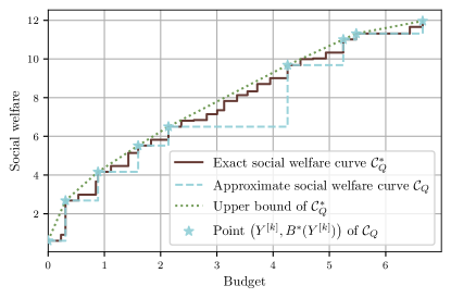
Figure 2: Distance between the social welfare curve $\mathcal{C}_{Q}$ computed by Algorithm 1, the maximum social welfare curve $\mathcal{C}^{*}_{Q}$ (Section II-C) and the upper bound of Theorem III-B.1. The stars represent the incentive spent $Y^{[k]}$ and social welfare $Y^{[k]}=B^{*}(Y^{[k]})$ at each iteration $k=1,\dots,8$ of the algorithm (line 9).

Fig. 2 illustrates the property above in a small example.

Proposition III-B.3.

The computational complexity of Alg. 1 is $O(\sum_{i=1}^{m}|\mathcal{N}_{i}|\cdot\log|\mathcal{R}_{i}|+|\mathcal{R}|\cdot\log m)$, where $m$ is the number of individuals, $|\mathcal{N}_{i}|$ is the number of alternatives of individual $i$, $|\mathcal{R}_{i}|$ is the number of LP-extremes of individual $i$ and $|\mathcal{R}|\triangleq\sum_{i=1}^{m}|\mathcal{R}_{i}|$.

Note that, since the alternatives of each individual are independent of the others, the sets $\mathcal{R}_{i}$ can be computed in parallel, thus reducing even further the computation time.

Despite our algorithm being computationally efficient, there might be cases in which it is desirable to stop it prematurely, without waiting for it to completely terminate. This can be the case when a personalized-incentive policy must be computed on-the-fly, within tight time-constraints. The following properties ensure that our algorithm is suitable to this situation, which eases its practical adoption.

Remark III-B.4 (Anytime algorithm).

Alg. 1 is anytime: if we stop it prematurely at any iteration $k$, we get a valid solution for the Maximum Social Welfare and the Maximum Social Welfare Curve problems, with budget $Q^{\prime}=Y^{[k]}$.

Remark III-B.5 (Incremental use).

Another desirable property of Algorithm 1 is that we can build on a previously computed incentive allocation whenever new available budget becomes available, instead of recomputing the entire allocation from scratch. To explain this, let us suppose that we have a certain budget $Q$ and the algorithm returns the allocation $\{x_{i,j}\}_{i,j}$, spending the corresponding incentive amount $\tilde{Q}$. Suppose now that the available budget increases to $Q^{\prime}>Q$. In this case, in order to exploit the new additional budget, we can simply resume the algorithm from its last iteration and continue up to the furthest iteration such that $Y^{[k+1]}\leq Q^{\prime}$. This is, per-se, a computational advantage with respect to algorithms that need to run from scratch every time new resources (budget) are available.

IV Imperfect Information

The assumption that the regulator knows perfectly the utility of the individuals may seem restrictive. In this section, we show that the algorithm is still relevant when the utility is imperfectly known. From discrete-choice theory [10], we assume that intrinsic utility of alternative $j$ of individual $i$ is $V_{i,j}=\hat{V}_{i,j}+\epsilon_{i,j}$, where $\hat{V}_{i,j}$ is deterministic and $\epsilon_{i,j}$ randomly Gumbel-distributed. Their specific parameters are specified in our code [7].

We assume that the regulator knows the deterministic part $\hat{V}_{i,j}$ of the utility but not the random part $\epsilon_{i,j}$.

Under this assumption, the regulator does not know the minimum incentive amount needed to induce individual $i$ to shift from her default alternative $j^{0}_{i}$ to another alternative $j$. A heuristic solution would be to set the incentive amount equal to the expectation of the utility difference between the two alternatives, given that $j^{0}_{i}$ is the default alternative chosen when there is no incentive. In this case, the incentives $\{y_{i,j}\}_{j\in\mathcal{N}_{i}}$ proposed by the regulator to individual $i$, to convince her to shift to alternative $j$, are such that $y_{i,{j^{\prime}}}=0$, for any ${j^{\prime}}\neq j$, and

$$y_{i,j}= \mathbb{E}(V_{i,j^{0}_{i}}-V_{i,j}|V_{i,j^{0}_{i}}>V_{i,j})=$$ (10)

$$\hat{y}_{i,j}+\mathbb{E}(\epsilon_{i,j^{0}_{i}}-\epsilon_{i,j}|\epsilon_{i,j^{0}_{i}}-\epsilon_{i,j}>-\hat{y}_{i,j}),$$ (11)

where $\hat{y}_{i,j}=\hat{V}_{i,j^{0}_{i}}-\hat{V}_{i,j}$ is the difference in the deterministic part of the utility, known to the regulator.

Given an individual $i$ and an alternative $j\in\mathcal{N}_{i}$, if the regulator proposes the incentive $y_{i,j}$, as defined by (10), then individual $i$ has a positive probability to refuse the incentive. Hence, the expenses of the regulator may be smaller than the total incentive amount proposed.

Algorithm 1 can be used to compute a personalized-incentive policy under imperfect information, by defining new weights

$$w_{i,j}=\mathbb{E}(V_{i,j^{0}_{i}}-V_{i,j}|V_{i,j^{0}_{i}}>V_{i,j}).$$

At each iteration of the algorithm, the regulator proposes the incentive $w_{i^{\prime},j^{\prime}}$ to individual $i^{\prime}$ for alternative $j^{\prime}$, where $[i^{\prime},j^{\prime}]$ is the pair of individual and alternative selected by the algorithm. The regulator observes the response of the individual to the incentive. If the individual accepts the incentive, it decreases the budget by the incentive amount. The regulator keeps proposing incentives one by one until his budget is depleted.

Note that, if an individual $i$ accepts an incentive $y_{i,j}$ for alternative $j\in\mathcal{N}_{i}$, the regulator can still propose her, later, an incentive $y_{i,{j^{\prime}}}$ for another alternative ${j^{\prime}}\in\mathcal{N}_{i}$. If the individual refuses the second incentive $y_{i,{j^{\prime}}}$, she still receives the first incentive $y_{i,j}$.

In Section V-B, we apply the policy presented above to our case study and compare it to the case with perfect information, assuming that random terms are Gumbel-distributed. The following proposition gives the exact expression of the incentives (10), in case of Gumbel-distributed random terms.

Proposition IV-.1.

Let us assume that the random terms are i.i.d. and follow a Gumbel distribution with scale parameter $\mu$ (i.e., $\epsilon_{i,j}/\mu$ follows a standard Gumbel distribution). Then, the incentive amount from (10) can be written as

$$y_{i,j}=\mu\frac{1+e^{\hat{y}_{i,j}/\mu}}{e^{\hat{y}_{i,j}/\mu}}\ln\left(1+e^{\hat{y}_{i,j}/\mu}\right)\geq 0.$$

V Application to Mode Choice

We consider a regulator willing to employ a limited monetary budget in order to promote eco-friendly modes of transportation in order to reduce CO₂ emissions.

Observed variables include city- or district-level home and work location, main mode of transportation used for commuting, and some socio-demographic variables. The modes of transportation are: car, public transit, walking, cycling and motorcycle. To estimate the utilities $V_{i,j}$ of each mode of transportation perceived by each individual, we resort to multinomial logit modeling on census data on the Rhône department ($222\,000$ households) from the French statistics institute INSEE in 2015-19. To estimate the social indicators $b_{i,j}$, we use data from the French Environmental Agency [11]. Details about the datasets and the estimation procedure can be found in our repository [7].

We implicitly assume that the utility and the social benefit of an individual when commuting by car or public transit does not depend on how many other individuals commute by car or by public transit. This approximation is legitimate if the number of modal shifts induced by the policy is low, so that their impact on congestion and occupation is negligible. We checked a posteriori that this latter assumption is verified in our case (less than $1.60\text{\,}\%$ of individuals shifted mode).

V-A Calculation of the Personalized-Incentive Policy

We have about $2\cdot 10^{5}$ individuals and $10^{6}$ alternatives. The regulator proposes, each day, incentives to the individuals before their home-work trip. The social indicator of an alternative is the reduction in CO₂ emissions for the trip back and forth, with respect to the default alternative. The budget is the daily amount available to the regulator. The social welfare curve given by Alg. 1 when daily budget is $3000$ € is in Fig. 3.

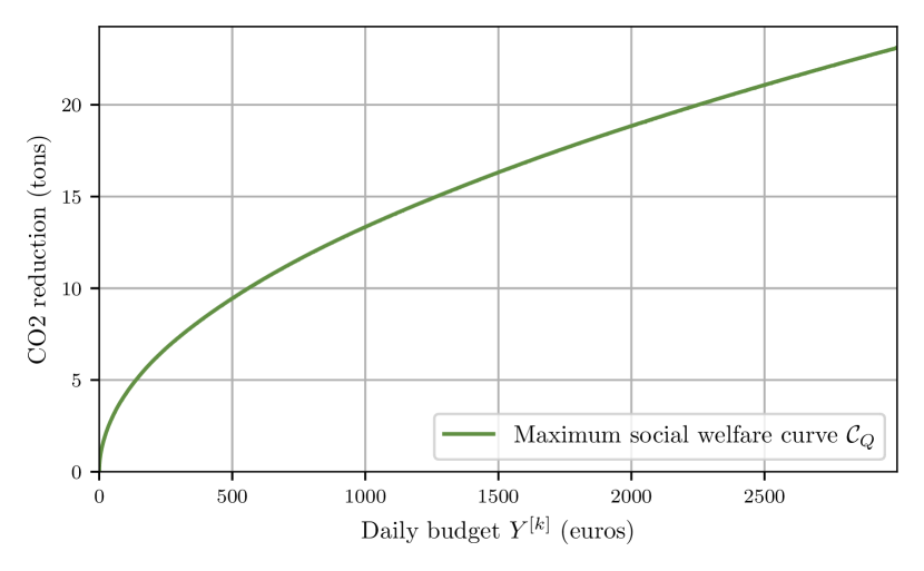
Figure 3: Maximum social welfare curve, up to a daily budget of 3000 €. Note: The social welfare corresponds to the reduction in CO₂ emissions due to the personalized-incentive policy.

We then set the budget of the regulator to $Q=$1800$$ €. Running Algorithm 1 with this budget required about $3500$ iterations and took about 6 seconds (with Python, on a computer with an Intel i5-8350U 1.7GHz and 24GB of memory). The algorithm allocates practically all the budget ($1798.59$ €), inducing modal shift of $1.57$% of individuals and CO₂ reduction by $18$ tons per day ($3.00\text{\,}\%$ of total CO₂ emissions). Thus, this policy would cost on average $100.61$ € for each ton of CO₂ prevented, which is a reasonable carbon price [12].

Despite the small incentives, the reduction in CO₂ emissions is considerable. Indeed, among the individuals who received incentives, the average amount of incentives is $0.52$ € per individual, for an average daily reduction in CO₂ emissions of $5$ kilograms. Recall that alternatives providing a large reduction in CO₂, while requiring small incentive, have a high efficiency. Hence, the algorithm selects first shifts achievable with a small incentive, i.e., where the individual is almost indifferent between the two alternatives, which however have a large difference in CO₂. Fig.4 shows the distribution of the incentive amount and the CO₂ reduction for the incentivized individuals. For most incentives, the amount proposed to individuals is below $1$ euro (larger incentives are rarely efficient).

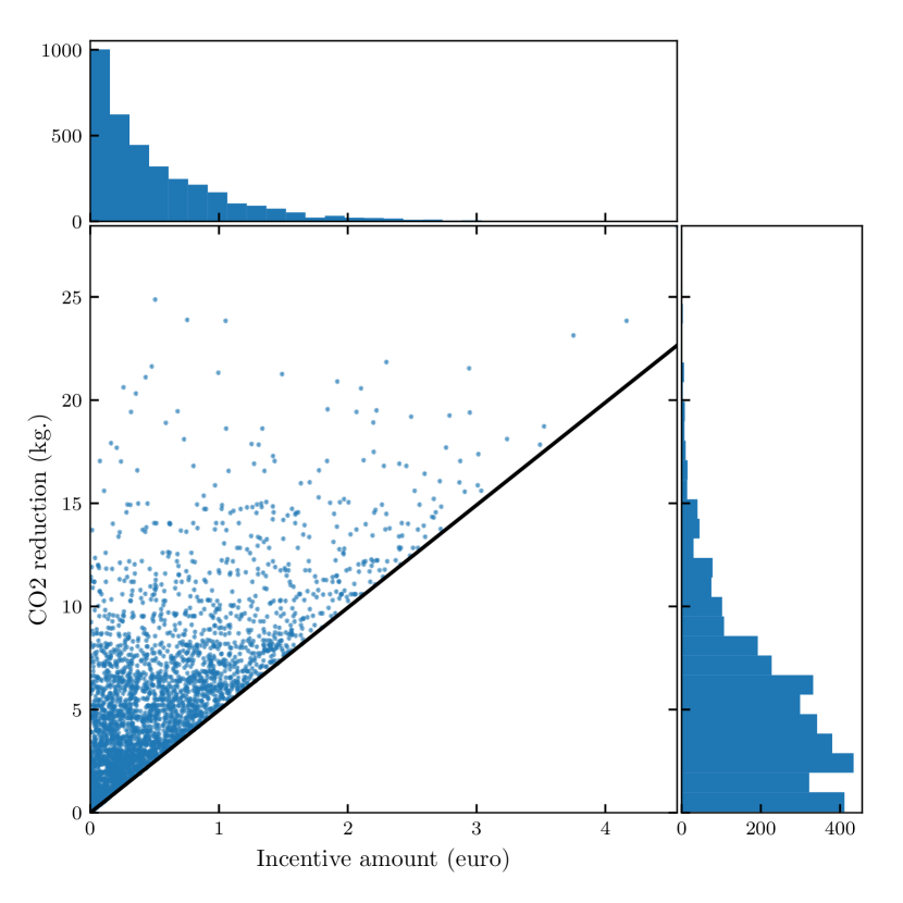
Figure 4: Distribution of incentive amount and CO₂ reduction for the incentives given in one day with budget $Q=1800$ €.
The slope of the black line represents the incremental efficiency of the split item returned by the algorithm, $\tilde{e}_{s,t}=$5$$ tons of CO₂ / euro. Note that all points are above the line because their incremental efficiency is larger. The histogram above represents the distribution of the incentive amounts. The histogram on the right represents the distribution of the CO₂ reduction for the incentives.

Fig.5 compares mode share before and after the policy. Most individuals who received incentives are individuals who commuted by car and were induced to commute by public transit ($1.2$% of all individuals, $74$% of individuals who received incentives). The share of individuals commuting by car decreased by 2.4%, while public transit ridership increased by $4$%.

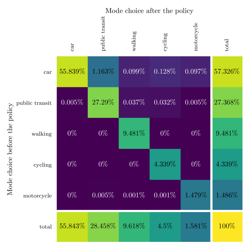
Figure 5: Evolution of mode share before and after the policy. $1.163\text{\,}\%$ of individuals were given incentives to shift from car to public transit, $27.29\text{\,}\%$ of individuals commuted by public transit before the policy and were not induced to shift.

We now compute a bound of the optimality gap, i.e., the maximum additional CO₂ savings we would achieve if we could use a theoretical optimal policy instead of resorting to Algorithm 1 (Theor. III-B.1). Since the incremental efficiency of the split item returned by the algorithm is $\tilde{e}_{s,t}\simeq 5$ kilograms of CO₂ per euro and the unused budget is $Q-\tilde{Q}=1.41$ €, an optimal policy would reduce of just $5\cdot 1.41\simeq 7$ kilograms more than Algorithm 1, which is negligible compared to the total CO₂ emissions reduction of $18$ tons provided overall.

V-B Imperfect Information

We show in this section the performance of our allocation policy when the regulator has imperfect information about individual utilities. In this case, the allocation policy is computed as in Section IV. Using the values of the random variables $\epsilon_{i,j}$ drawn previously, we can check whether individuals accept the incentives proposed to them. The policy stops when the daily budget of $1800$ € is depleted.

TABLE I: Performance of the personalized-incentive policy for one day, with perfect and imperfect information.

	Perfect information	Imperfect information
Budget spent	$1798.59$ €	$1797.03$ €
Incentives proposed	$3486$	$419$
Incentives accepted	$3486$	$247$
Acceptance rate	$100\text{\,}\%$	$59\text{\,}\%$
CO2 reduction	$17.9$ tons	$3.8$ tons

Table I compares the performance of our personalized-incentive policy under perfect and imperfect information. As expected, imperfect information decreases the efficacy of the policy. Since the regulator does not exactly know the individual utilities, it may propose insufficient incentives, which are rejected by individuals (it happens $41\text{\,}\%$ of the times). This results in a smaller reduction of CO₂ ($21\text{\,}\%$ compared with the perfect information case). Note that less individuals are involved in the incentive program (only $12\text{\,}\%$ compared to the perfect information case) because incentive given to single individuals are on average larger, and thus the budget is depleted more quickly.

These results could be improved by learning from the responses of individual $i$ to the incentives proposed earlier in order to compute the incentives that will be proposed to her for other alternatives. For example, if the regulator observes that individual $i$ refused the incentive to shift from car to walking, he learns information on the random term of the utility for car of individual $i$.

Also, if it is not possible to propose incentives to individual $i$ for different alternatives consecutively, the regulator could propose incentives for multiple alternatives simultaneously.

These extensions cannot be carried out with Algorithm 1. Future work could study the optimal personalized-incentive policy under imperfect information.

VI Conclusion

This paper explores a computationally efficient method for the regulator to determine the optimal incentives to be provided to each individual to alter their choices in order to maximize social welfare. Such a method requires to know the preferences of individuals, which could be possible, thanks to the wealth of data available for user nowadays, in compliance to privacy. We will more systematically study in our future work the imperfect information case, which we have here tackled empirically. Moreover, we will consider the possible congestion induced by the distribution of incentives, possibly via an iterative procedure alternating the incentive algorithm and the computation of the current level of congestion.

VII Acknowledgement

This work has been supported by The French ANR research project MuTAS (ANR-21-CE22-0025-01).

References

- [1] A. Clarke and H. Margetts, “Governments and citizens getting to know each other? open, closed, and big data in public management reform,” Policy & Internet, vol. 6, no. 4, pp. 393–417, 2014.
- [2] J. Sun et al., “Managing bottleneck congestion with incentives,” Transportation Research Part B: Methodological, 2020.
- [3] Y. Tang, Y. Jiang, H. Yang, and O. A. Nielsen, “Modeling and optimizing a fare incentive strategy to manage queuing and crowding in mass transit systems.” Tr.Res. Part B, 2020.
- [4] A. Araldo, M. Ben-Akiva et al., “System-level optimization of multi-modal transportation networks for energy efficiency using personalized incentives,” Transportation Research Records, vol. 2673, no. 12, 2019.
- [5] A. Colorni et al., “Rethinking feasibility analysis for urban development: A multidimensional decision support tool,” in ICCSA, 2017.
- [6] A. Araldo et al., “Resource Allocation for Edge Computing with Multiple Tenant Configurations,” in ACM/SIGAPP SAC, 2020.
- [7] L. Javaudin, “Code,” https://github.com/LucasJavaudin/individualized-incentives-algorithm, 2022.
- [8] H. Kellerer et al., Knapsack Problems, 1st ed. Springer, 2004.
- [9] A. A. Zoltners et al., “An Optimal Algorithm for Sales Representative Time Management,” Management Science, 1979.
- [10] S. P. Anderson, A. de Palma, and J. F. Thisse, Discrete choice theory of product differentiation. MIT press, 1992.
- [11] “Resource centre for greenhouse gas accounting,” https://www.bilans-ges.ademe.fr/en/.
- [12] A. Quinet et al., “La valeur tutélaire du carbone,” Rapport du Conseil d’Analyse Stratégique, 2009.