Improved Stein Variational Gradient Descent with Importance Weights

Abstract

Stein Variational Gradient Descent ( SVGD) is a popular sampling algorithm used in various machine learning tasks. It is well known that SVGD arises from a discretization of the kernelized gradient flow of the Kullback-Leibler divergence $D_{\mathrm{KL}}\left(\cdot\mid\pi\right)$, where $\pi$ is the target distribution. In this work, we propose to enhance SVGD via the introduction of importance weights, which leads to a new method for which we coin the name $\beta$-SVGD. In the continuous time and infinite particles regime, the time for this flow to converge to the equilibrium distribution $\pi$, quantified by the Stein Fisher information, depends on $\rho_{0}$ and $\pi$ very weakly. This is very different from the kernelized gradient flow of Kullback-Leibler divergence, whose time complexity depends on $D_{\mathrm{KL}}\left(\rho_{0}\mid\pi\right)$. Under certain assumptions, we provide a descent lemma for the population limit $\beta$-SVGD, which covers the descent lemma for the population limit SVGD when $\beta\to 0$. We also illustrate the advantages of $\beta$-SVGD over SVGD by experiments.

1 Introduction

The main technical task of Bayesian inference is to estimate integration with respect to the posterior distribution

$$\pi(x)\propto e^{-V(x)},$$

where $V:\mathbb{R}^{d}\to\mathbb{R}$ is a potential. In practice, this is often reduced to sampling points from the distribution $\pi$. Typical methods that employ this strategy include algorithms based on Markov Chain Monte Carlo ( MCMC), such as Hamiltonian Monte Carlo (Neal, 2011), also known as Hybrid Monte Carlo ( HMC) (Duane et al., 1987; Betancourt, 2017), and algorithms based on Langevin dynamics (Dalalyan & Karagulyan, 2019; Durmus & Moulines, 2017; Cheng et al., 2018).

One the other hand, Stein Variational Gradient Descent ( SVGD)—a different strategy suggested by Liu & Wang (2016)—is based on an interacting particle system. In the population limit, the interacting particle system can be seen as the kernelized negative gradient flow of the Kullback-Leibler divergence

$$\textstyle D_{\mathrm{KL}}\left(\rho\mid\pi\right):=\int\log\left(\frac{\rho}{\pi}\right)(x)\;d\rho(x);$$ (1)

see (Liu, 2017; Duncan et al., 2019). SVGD has already been widely used in a variety of machine learning settings, including variational auto-encoders (Pu et al., 2017), reinforcement learning (Liu et al., 2017), sequential decision making (Zhang et al., 2018; 2019), generative adversarial networks (Tao et al., 2019) and federated learning (Kassab & Simeone, 2022). However, current theoretical understanding of SVGD is limited to its infinite particle version (Liu, 2017; Korba et al., 2020; Salim et al., 2021; Sun et al., 2022), and the theory on finite particle SVGD is far from satisfactory.

Since SVGD is built on a discretization of the kernelized negative gradient flow of (1), we can learn about its sampling potential by studying this flow. In fact, a simple calculation reveals that

$$\textstyle\min\limits_{0\leq s\leq t}I_{Stein}\left(\rho_{s}\mid\pi\right)\leq\frac{D_{\mathrm{KL}}\left(\rho_{0}\mid\pi\right)}{t},$$ (2)

where $I_{Stein}\left(\rho_{s}\mid\pi\right)$ is the Stein Fisher information (see Definition 2) of $\rho_{s}$ relative to $\pi$, which is typically used to quantify how close to $\pi$ are the probability distributions $\left(\rho_{s}\right)_{s=0}^{t}$ generated along this flow. In particular, if our goal is to guarantee $\min\limits_{0\leq s\leq t}I_{Stein}\left(\rho_{s}\mid\pi\right)\leq\varepsilon,$ result (2) says that we need to take

$$\textstyle t\geq\frac{D_{\mathrm{KL}}\left(\rho_{0}\mid\pi\right)}{\varepsilon}.$$

Unfortunately, and this is the key motivation for our work, the quantity the initial $\operatorname{KL}$ divergence $D_{\mathrm{KL}}\left(\rho_{0}\mid\pi\right)$ can be very large. Indeed, it can be proportional to the underlying dimension, which is highly problematic in high dimensional regimes. Salim et al. (2021) and Sun et al. (2022) have recently derived an iteration complexity bound for the infinite particle SVGD method. However, similarly to the time complexity of the continuous flow, their bound depends on $D_{\mathrm{KL}}\left(\rho_{0}\mid\pi\right)$.

1.1 Summary of contributions

In this paper, we design a family of continuous time flows—which we call $\beta$-SVGD flow—by combining importance weights with the kernelized gradient flow of the $\operatorname{KL}$-divergence. Surprisingly, we prove that the time for this flow to converge to the equilibrium distribution $\pi$, that is $\min_{0\leq s\leq t}I_{Stein}\left(\rho_{s}\mid\pi\right)\leq\varepsilon$ with $(\rho_{s})_{s=0}^{t}$ generated along $\beta$-SVGD flow, can be bounded by $-\frac{1}{\varepsilon\beta(\beta+1)}$ when $\beta\in(-1,0)$. This indicates that the importance weights can potentially accelerate SVGD. Actually, we design $\beta$-SVGD method based on a discretization of the $\beta$-SVGD flow and provide a descent lemma for its population limit version. Some simple experiments in Appendix D verify our predictions.

We summarize our contributions in the following:

• A new family of flows. We construct a family of continuous time flows for which we coin the name $\beta$-SVGD flows. These flows do not arise from a time re-parameterization of the SVGD flow since their trajectories are different, nor can they be seen as the kernelized gradient flows of the Rényi divergence.

• Convergence rates. When $\beta\to 0$, this returns back to the kernelized gradient flow of the $\operatorname{KL}$-divergence ( SVGD flow); when $\beta\in(-1,0)$, the convergence rate of $\beta$-SVGD flows is significantly improved than that of the SVGD flow in the case $D_{\mathrm{KL}}\left(\rho_{0}\mid\pi\right)$ is large. Under a Stein Poincaré inequality, we derive an exponential convergence rate of $2$-Rényi divergence along $1$-SVGD flow. Stein Poincaré inequality is proved to be weaker than Stein log-Sobolev inequality, however like Stein log-Sobolev inequality, it is not clear to us when it does hold.

• Algorithm. We design $\beta$-SVGD algorithm based on a discretization of the $\beta$-SVGD flow and we derive a descent lemmas for the population limit $\beta$-SVGD.

• Experiments. Finally, we do some experiments to illustrate the advantages of $\beta$-SVGD with negative $\beta$. The simulation results on $\beta$-SVGD corroborate our theory.

1.2 Related works

The SVGD sampling technique was first presented in the fundamental work of Liu & Wang (2016). Since then, a number of SVGD variations have been put out. The following is a partial list: Newton version SVGD (Detommaso et al., 2018), stochastic SVGD (Gorham et al., 2020), mirrored SVGD (Shi et al., 2021), random-batch method SVGD (Li et al., 2020) and matrix kernel SVGD (Wang et al., 2019). The theoretical knowledge of SVGD is still constrained to population limit SVGD. The first work to demonstrate the convergence of SVGD in the population limit was by Liu (2017); Korba et al. (2020) then derived a similar descent lemma for the population limit SVGD using a different approach. However, their results relied on the path information and thus were not self-contained, to provide a clean analysis, Salim et al. (2021) assumed a Talagrand’s $T_{1}$ inequality of the target distribution $\pi$ and gave the first iteration complexity analysis in terms of dimension $d$. Following the work of Salim et al. (2021); Sun et al. (2022) derived a descent lemma for the population limit SVGD under a non-smooth potential $V$.

In this paper, we consider a family of generalized divergences, Rényi divergence, and SVGD with importance weights. For these two themes, we name a few but non-exclusive related results. Wang et al. (2018) proposed to use the $f$-divergence instead of $\operatorname{KL}$-divergence in the variational inference problem, here $f$ is a convex function; Yu et al. (2020) also considered variational inference with $f$-divergence but with its dual form. Han & Liu (2017) considered combining importance sampling with SVGD, however the importance weights were only used to adjust the final sampled points but not in the iteration of SVGD as in this paper; Liu & Lee (2017) considered importance sampling, they designed a black-box scheme to calculate the importance weights (they called them Stein importance weights in their paper) of any set of points.

2 Preliminaries

We assume the target distribution $\pi\propto e^{-V}$, and we have oracle to calculate the value of $e^{-V(x)}$ for all $x\in\mathbb{R}^{d}$.

2.1 Notation

Let $x=\left(x_{1},\ldots,x_{d}\right)^{\top},y=\left(y_{1},\ldots,y_{d}\right)^{\top}\in\mathbb{R}^{d}$, denote $\left<x,y\right>:=\sum_{i=1}^{d}x_{i}y_{i}$ and $\left\|x\right\|:=\sqrt{\left<x,x\right>}$. For a square matrix $B\in\mathbb{R}^{d\times d}$, the operator norm and Frobenius norm of $B$ are defined respectively by $\|B\|_{op}:=\sqrt{\varrho(B^{\top}B)}$ and $\|B\|_{F}:=\sqrt{\sum_{i=1}^{d}\sum_{j=1}^{d}B_{i,j}^{2}}$, respectively, where $\varrho$ denotes the spectral radius. It is easy to verify that $\left\|B\right\|_{op}\leq\left\|B\right\|_{F}$. Let ${\mathcal{P}}_{2}(\mathbb{R}^{d})$ denote the space of probability measures with finite second moment; that is, for any $\mu\in{\mathcal{P}}_{2}(\mathbb{R}^{d})$ we have $\int\left\|x\right\|^{2}\;d\mu(x)<+\infty$. The Wasserstein $2$-distance between $\rho,\mu\in{\mathcal{P}}_{2}(\mathbb{R}^{d})$ is defined by

$$\textstyle W_{2}\left(\rho,\mu\right):=\inf\limits_{\eta\in\Gamma(\rho,\mu)}\sqrt{\int\left\|x-y\right\|^{2}\;d\eta(x,y)},$$

where $\Gamma\left(\rho,\mu\right)$ is the set of all joint distributions defined on $\mathbb{R}^{d}\times\mathbb{R}^{d}$ having $\rho$ and $\mu$ as marginals. The push-forward distribution of $\rho\in{\mathcal{P}}_{2}\left(\mathbb{R}^{d}\right)$ by a map $T:\mathbb{R}^{d}\to\mathbb{R}^{d}$, denoted by $T_{\#}\rho$, is defined as follows: for any measurable set $\Omega\in\mathbb{R}^{d}$, $T_{\#}\rho\left(\Omega\right):=\rho\left(T^{-1}\left(\Omega\right)\right)$. By definition of the push-forward distribution, it is not hard to verify that the probability densities satisfy $T_{\#}\rho(T(x))|\operatorname{det}\operatorname{D}T(x)|=\rho(x)$, where $\operatorname{D}T$ is the Jacobian matrix of $T$. The reader can refer to Villani (2009) for more details.

2.2 Rényi divergence

Next, we define the Rényi divergence which plays an important role in information theory and many other areas such as hypothesis testing (Morales González et al., 2013) and multiple source adaptation (Mansour et al., 2012).

Definition 1 (Rényi divergence)

For two probability distributions $\rho$ and $\mu$ on $\mathbb{R}^{d}$ and $\rho\ll\mu$, the Rényi divergence of positive order $\alpha$ is defined as

$$\mathop{\mathrm{D}_{\alpha}}\nolimits(\rho\mid\mu):=\begin{cases}\frac{1}{\alpha-1}\log\left(\int\left(\frac{\rho}{\mu}\right)^{\alpha-1}(x)\;d\rho(x)\right)&0<\alpha<\infty,\;\alpha\neq 1\\ \int\log\left(\frac{\rho}{\mu}\right)(x)\;d\rho(x)&\alpha=1\end{cases}.$$ (3)

If $\rho$ is not absolutely continuous with respect to $\mu$, we set $\mathop{\mathrm{D}_{\alpha}}\nolimits(\rho\mid\mu)=\infty$. Further, we denote $D_{\mathrm{KL}}\left(\rho\mid\mu\right):=\mathrm{D}_{1}\left(\rho\mid\mu\right)$.

Rényi divergence is non-negative, continuous and non-decreasing in terms of the parameter $\alpha$; specifically, we have $D_{\mathrm{KL}}\left(\rho\mid\mu\right)=\lim_{\alpha\to 1}\mathop{\mathrm{D}_{\alpha}}\nolimits(\rho\mid\mu)$. More properties of Rényi divergence can be found in a comprehensive article by Van Erven & Harremos (2014). Besides Rényi divergence, there are other generalizations of the $\operatorname{KL}$-divergence, e.g., admissible relative entropies (Arnold et al., 2001).

2.3 Background on SVGD

Stein Variational Gradient Descent ( SVGD) is defined on a Reproducing Kernel Hilbert Space (RKHS) ${\mathcal{H}}_{0}$ with a non-negative definite reproducing kernel $k:\mathbb{R}^{d}\times\mathbb{R}^{d}\to\mathbb{R}^{+}$. The key feature of this space is its reproducing property:

$$f(x)=\left<f(\cdot),k(x,\cdot)\right>_{{\mathcal{H}}_{0}},\qquad\forall f\in{\mathcal{H}}_{0},$$ (4)

where $\left<\cdot,\cdot\right>_{{\mathcal{H}}_{0}}$ is the inner product defined on ${\mathcal{H}}_{0}$. Let ${\mathcal{H}}$ be the $d$-fold Cartesian product of ${\mathcal{H}}_{0}$. That is, $f\in{\mathcal{H}}$ if and only if there exist $f_{1},\cdots,f_{d}\in{\mathcal{H}}_{0}$ such that $f=\left(f_{1},\ldots,f_{d}\right)^{\top}$. Naturally, the inner product on ${\mathcal{H}}$ is given by

$$\textstyle\left<f,g\right>_{{\mathcal{H}}}:=\sum\limits_{i=1}^{d}\left<f_{i},g_{i}\right>_{{\mathcal{H}}_{0}},\qquad f=\left(f_{1},\ldots,f_{d}\right)^{\top}\in{\mathcal{H}},\qquad g=\left(g_{1},\ldots,g_{d}\right)^{\top}\in{\mathcal{H}}.$$ (5)

For more details of RKHS, the readers can refer to Berlinet & Thomas-Agnan (2011).

It is well known (see for example Ambrosio et al. (2005)) that $\nabla\log\left(\frac{\rho}{\pi}\right)$ is the Wasserstein gradient of $D_{\mathrm{KL}}\left(\cdot\mid\pi\right)$ at $\rho\in{\mathcal{P}}_{2}(\mathbb{R}^{d})$. Liu & Wang (2016) proposed a kernelized Wasserstein gradient of the $\operatorname{KL}$-divergence, defined by

$$\textstyle g_{\rho}(x):=\int k(x,y)\nabla\log\left(\frac{\rho}{\pi}\right)(y)\;d\rho(y)\in{\mathcal{H}}.$$ (6)

Integration by parts yields

$$\textstyle g_{\rho}(x)=-\int\left[\nabla\log\pi(y)k(x,y)+\nabla_{y}k(x,y)\right]\;d\rho(y).$$ (7)

Comparing the Wasserstein gradient $\nabla\log\left(\frac{\rho}{\pi}\right)$ with (7), we find that the latter can be easily approximated by

$$\textstyle g_{\rho}(x)\approx\hat{g}_{\hat{\rho}}:=-\frac{1}{N}\sum\limits_{i=1}^{N}\left[\nabla\log\pi(x_{i})k(x,x_{i})+\nabla_{x_{i}}k(x,x_{i})\right],$$ (8)

with $\hat{\rho}=\frac{1}{N}\sum_{i=1}^{N}\delta_{x_{i}}$ and $\left(x_{i}\right)_{i=1}^{N}$ sampled from $\rho$. With the above notations, the SVGD update rule

$$\textstyle x_{i}\leftarrow x_{i}+\frac{\gamma}{N}\sum\limits_{j=1}^{N}\left[\nabla\log\pi(x_{j})k(x_{i},x_{j})+\nabla_{x_{j}}k(x_{i},x_{j})\right],\quad i=1,\ldots,N,$$ (9)

where $\gamma$ is the step-size, can be presented in the compact form $\hat{\rho}\leftarrow\left(I-\gamma\hat{g}_{\hat{\rho}}\right)_{\#}\hat{\rho}.$ When we talk about the infinite particle SVGD, or population limit SVGD, we mean $\rho\leftarrow\left(I-\gamma{g}_{\rho}\right)_{\#}\rho.$ The metric used in the study of SVGD is the Stein Fisher information or the Kernelized Stein Discrepancy (KSD).

Definition 2 (Stein Fisher Information)

Let $\rho\in\mathcal{P}_{2}(\mathbb{R}^{d})$. The Stein Fisher Information of $\rho$ relative to $\pi$ is defined by

$$\textstyle I_{Stein}(\rho\mid\pi):=\iint k(x,y)\left<\nabla\log\left(\frac{\rho}{\pi}\right)(x),\nabla\log\left(\frac{\rho}{\pi}\right)(y)\right>\;d\rho(x)\;d\rho(y).$$ (10)

A sufficient condition under which $\lim_{n\to\infty}I_{Stein}(\rho_{n}\mid\pi)$ implies $\rho_{n}\to\pi$ weakly can be found in Gorham & Mackey (2017), which requires: i) the kernel $k$ to be in the form $k(x,y)=\left(c^{2}+\left\|x-y\right\|^{2}\right)^{\theta}$ for some $c>0$ and $\theta\in(-1,0)$; ii) $\pi\propto e^{-V}$ to be distant dissipative; roughly speaking, this requires $V$ to be convex outside a compact set, see Gorham & Mackey (2017) for an accurate definition.

In the study of the kernelized Wasserstein gradient (7) and its corresponding continuity equation

$$\textstyle\frac{\partial\rho_{t}}{\partial t}+\operatorname{div}\left(\rho_{t}g_{\rho_{t}}\right)=0,$$

Duncan et al. (2019) introduced the following kernelized log-Sobolev inequality to prove the exponential convergence of $D_{\mathrm{KL}}\left(\rho_{t}\mid\pi\right)$ along the direction (7):

Definition 3 (Stein log-Sobolev inequality)

We say $\pi$ satisfies the Stein log-Sobolev inequality with constant $\lambda>0$ if

$$\textstyle D_{\mathrm{KL}}(\rho\mid\pi)\leq\frac{1}{2\lambda}I_{Stein}(\rho\mid\pi).$$ (11)

While this inequality can guarantee an exponential convergence rate of $\rho_{t}$ to $\pi$, quantified by the $\operatorname{KL}$-divergence, the condition for $\pi$ to satisfy the Stein log-Sobolev inequality is very restrictive. In fact, little is known about when (11) holds.

3 Continuous time dynamics of the $\beta$-SVGD flow

In this section, we mainly focus on the continuous time dynamics of the $\beta$-SVGD flow. Due to page limitation, we leave all of the proofs to Appendix B.

3.1 $\beta$-SVGD flow

In this paper, a flow refers to some time-dependent vector field $v_{t}:\mathbb{R}^{d}\to\mathbb{R}^{d}$. This time-dependent vector field will influence the mass distribution on $\mathbb{R}^{d}$ by the continuity equation or the equation of conservation of mass

$$\textstyle\frac{\partial\rho_{t}}{\partial t}+\operatorname{div}\left(\rho_{t}v_{t}\right)=0,$$ (12)

readers can refer to Ambrosio et al. (2005) for more details.

Definition 4 ( $\beta$-SVGD flow)

Given a weight parameter $\beta\in(-1,+\infty)$, the $\beta$-SVGD flow is given by

$$\textstyle v_{t}^{\beta}(x):=-\left(\frac{\pi}{\rho_{t}}\right)^{\beta}(x)\int k(x,y)\nabla\log\left(\frac{\rho_{t}}{\pi}\right)(y)\;d\rho_{t}(y).$$ (13)

Note that when $\beta=0$, this is the negative kernelized Wasserstein gradient (6).

Note that we can not treat $\beta$-SVGD flow as the kernelized Wasserstein gradient flow of the $(\beta+1)$-Rényi divergence. However, they are closely related, and we can derive the following theorem.

Theorem 1 (Main result)

Along the $\beta$-SVGD flow (13), we have

$$\min_{t\in[0,T]}I_{Stein}\left(\rho_{t}\mid\pi\right)\leq\frac{1}{T}\int_{0}^{T}I_{Stein}(\rho_{t}\mid\pi)dt\leq\begin{cases}\frac{e^{\beta\mathrm{D}_{\beta+1}\left(\rho_{0}\mid\pi\right)}}{T\beta(\beta+1)}&\beta>0\\ \frac{D_{\mathrm{KL}}(\rho_{0}\mid\pi)}{T}&\beta=0\\ -\frac{1}{T\beta(\beta+1)}&\beta\in(-1,0)\end{cases}.$$ (14)

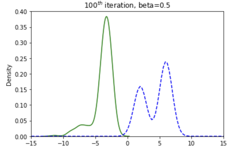
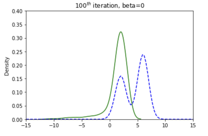
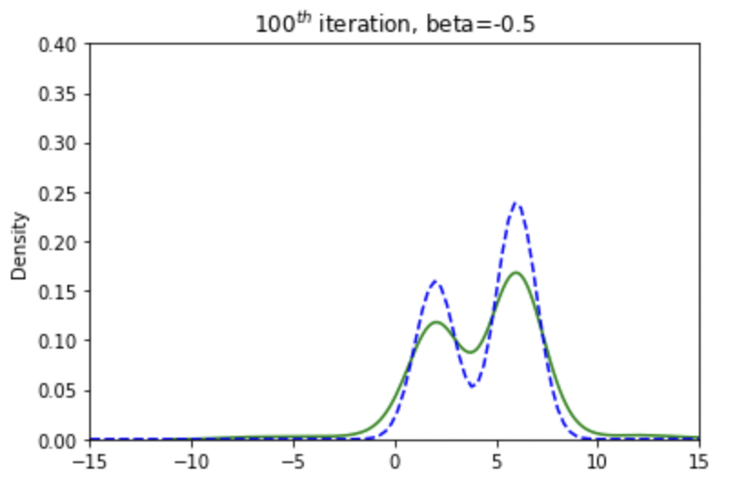
Figure 1: The performance of $\beta$-SVGD with $\beta=0.5,0,-0.5$ from left to right, but with the same step-size. The blue dashed line is the target distribution $\pi$: the Gaussian mixture $\frac{2}{5}{\mathcal{N}}(2,1)+\frac{3}{5}{\mathcal{N}}(6,1)$. The green solid line is the distribution generated by $\beta$-SVGD after 100 iterations; More experiments can be found in Appendix D.

Note the left hand side of (14) is the Stein Fisher information. When $\beta$ decreases from positive to negative, the right hand side of (14) changes dramatically; it appears to be independent of $\rho_{0}$ and $\pi$. If we do not know the Rényi divergence between $\rho_{0}$ and $\pi$, it seems the best convergence rate is obtained by setting $\beta=-\frac{1}{2}$, that is

$$\textstyle\min_{t\in[0,T]}I_{Stein}\left(\rho_{t}\mid\pi\right)\leq\frac{1}{T}\int_{0}^{T}I_{Stein}(\rho_{t}\mid\pi)dt\leq\leq\frac{4}{T}.$$

It is somewhat unexpected to observe that the time complexity is independent of $\rho_{0}$ and $\pi$, or to be more precise, that it relies only very weakly on $\rho_{0}$ and $\pi$ when $\beta\in(-1,0)$. We wish to stress that this is not achieved by time re-parameterization. In the proof of Theorem 1, we can see the term $\left(\nicefrac{{\pi}}{{\rho_{t}}}\right)^{\beta}$ in $\beta$-SVGD flow (13) is utilized to cancel term $\left(\nicefrac{{\rho_{t}}}{{\pi}}\right)^{\beta}$ in the Wasserstein gradient of $(\beta+1)$-Rényi divergence. Actually, when $\beta\in(-1,0)$, this term has an added advantage and can be seen as the acceleration factor in front of the kernelized Wasserstein gradient of $\operatorname{KL}$-divergence. Specifically, the negative kernelized Wasserstein gradient of $\operatorname{KL}$-divergence $v_{t}^{0}(x):=-\int k(x,y)\nabla\log(\frac{\rho_{t}}{\pi})(y)d\rho_{t}(y)$ is the vector field that compels $\rho_{t}$ to approach $\pi$, while $\left(\nicefrac{{\pi}}{{\rho_{t}}}\right)^{\beta}(x)$ is big (roughly speaking this means $x$ is close to the mass concentration region of $\rho_{t}$ but away from the one of $\pi$), this factor will enhance the vector field at point $x$ and force the mass around $x$ move faster towards the mass concentration region of $\pi$; on the other hand, if $\left(\nicefrac{{\pi}}{{\rho_{t}}}\right)^{\beta}(x)$ is small (this means $x$ is already near to the mass concentration region of $\pi$), this factor will weaken the vector field and make the mass surrounding $x$ remain within the mass concentration region of $\pi$. This is the intuitive justification for why, when $\beta\in(-1,0)$, the time complexity for $\beta$-SVGD flow to diminish the Stein Fisher information only depends on $\rho_{0}$ and $\pi$ very weakly.

Remark 1

While it may seem reasonable to suspect that the time complexity of the $\beta$-SVGD flow with $\beta\leq-1$ will also depend on $\rho_{0}$ and $\pi$ very weakly, surprisingly, this is not true. In fact, we can prove that (see Appendix B)

$$\textstyle\min_{t\in[0,T]}I_{Stein}\left(\rho_{t}\mid\pi\right)\leq\frac{1}{T}\int_{0}^{T}I_{Stein}(\rho_{t}\mid\pi)dt\leq\frac{e^{(-\beta-1)\mathrm{D}_{-\beta}\left(\pi\mid\rho_{0}\right)}}{|T\beta(\beta+1)|}.$$

Letting $\beta\to-1$, we get $\min_{t\in[0,T]}I_{Stein}\left(\rho_{t}\mid\pi\right)\leq\frac{D_{\mathrm{KL}}\left(\pi\mid\rho_{0}\right)}{T}$. The regime when $\beta\leq-1$ is similar to the $\beta>0$ regime in Theorem 1, which heavily depends on $\rho_{0}$ and $\pi$. Mathematically speaking, the weak dependence on $\rho_{0}$ and $\pi$ is caused by the concavity of the function $s^{\alpha}$ on $s\in\mathbb{R}^{+}$ when $\alpha=\beta+1\in(0,1)$.

3.2 1-SVGD flow and the Stein Poincaré inequality

Functional $D_{\mathrm{KL}}\left(\cdot\mid\cdot\right)$ is non-symmetric; that is, $D_{\mathrm{KL}}\left(\cdot\mid\pi\right)\neq D_{\mathrm{KL}}\left(\pi\mid\cdot\right)$, and so is their Wasserstein gradient. The Wasserstein gradient of $D_{\mathrm{KL}}\left(\pi\mid\cdot\right)$ at distribution $\rho\in{\mathcal{P}}_{2}(\mathbb{R}^{d})$ is $-\nabla\frac{\pi}{\rho}$ (see Appendix A), or, to put it another way, $\frac{\pi}{\rho}\nabla\log(\frac{\rho}{\pi})$, which may be regarded as the non-kernelized $1$-SVGD flow (module a minus sigh) when compared to (13). To conclude, the $1$-SVGD flow

$$\textstyle v_{t}^{1}(x):=-\frac{\pi}{\rho_{t}}(x)\int k(x,y)\nabla\log\left(\frac{\rho_{t}}{\pi}\right)(y)\;d\rho_{t}(y),$$ (15)

is the negative kernelized Wasserstein gradient flow of $D_{\mathrm{KL}}\left(\pi\mid\cdot\right)$. Next, we will study the exponential convergence of $2$-Rényi divergence along $1$-SVGD flow under the Stein Poincaré inequality.

Definition 5 (Stein Poincaré inequality)

We say that $\pi$ satisfies the Stein Poincaré inequality with constant $\lambda>0$ if

$$\textstyle\int|g|^{2}\;d\pi\leq\frac{1}{\lambda}\iint k(x,y)\left<\nabla g(x),\nabla g(y)\right>\;d\pi(x)\;d\pi(y),$$ (16)

for any smooth $g$ with $\int g\;d\pi=0$.

While Duncan et al. (2019) also introduced the Stein Poincaré inequality, they presented it in a different form. Just as Poincaré inequality is a linearized log-Sobolev inequality (see for example (Bakry et al., 2014, Proposition 5.1.3)), Stein Poincaré inequality is also a linearized Stein log-Sobolev inequality (11). Although Stein Poincaré inequality is weaker than Stein log-Sobolev inequality, the condition for it to hold is quite restrictive, as in the case of Stein log-Sobolev inequality; see the discussion in (Duncan et al., 2019, Section 6).

Lemma 1 (Stein log-Sobolev implies Stein Poincaré)

If $\pi$ satisfies the Stein log-Sobolev inequality (11) with constant $\lambda>0$, then it also satisfies the Stein Poincaré inequality with the same constant $\lambda$.

While the proof of the above lemma is a routine task, for completeness we provide it in Appendix B. The following theorem is inspired by Cao et al. (2019), in which they proved the exponential convergence of Rényi divergence along Langevin dynamic under a strongly convex potential $V$. However, due to the structure of $1$-SVGD flow, we can only prove the results for $\alpha$-Rényi divergence with $\alpha\in(0,2]$.

Theorem 2

Suppose $\pi$ satisfies the Stein Poincaré inequality with constant $\lambda>0$. Then the flow (15) satisfies

$$\mathop{\mathrm{D}_{2}}\nolimits\left(\rho_{t}\mid\pi\right)\leq C\cdot\mathop{\mathrm{D}_{2}}\nolimits\left(\rho_{0}\mid\pi\right)\cdot e^{-2\lambda t},$$ (17)

where $C=\frac{e^{\mathop{\mathrm{D}_{2}}\nolimits\left(\rho_{0}\mid\pi\right)}-1}{\mathop{\mathrm{D}_{2}}\nolimits\left(\rho_{0}\mid\pi\right)}$.

Since $\mathrm{D}_{\alpha_{1}}\left(\rho\mid\pi\right)\leq\mathrm{D}_{\alpha_{2}}\left(\rho\mid\pi\right)$ for any $0<\alpha_{1}\leq\alpha_{2}<\infty$, the exponential convergence of $\alpha$-Rényi divergence with $\alpha\in(0,2)$ can be easily deduced from (17).

Corollary 1

Suppose $\pi$ satisfies the Stein Poincaré inequality with constant $\lambda>0$. Then the flow (15) satisfies

$$\mathop{\mathrm{D}_{\alpha}}\nolimits\left(\rho_{t}\mid\pi\right)\leq C\cdot\mathop{\mathrm{D}_{\alpha}}\nolimits\left(\rho_{0}\mid\pi\right)\cdot e^{-2\lambda t}$$ (18)

for all $\alpha\in(0,2]$, where $C=\frac{e^{\mathop{\mathrm{D}_{2}}\nolimits\left(\rho_{0}\mid\pi\right)}-1}{\mathop{\mathrm{D}_{\alpha}}\nolimits\left(\rho_{0}\mid\pi\right)}$.

4 The $\beta$-SVGD algorithm

The $\beta$-SVGD algorithm proposed here is a sampling method suggested by the discretization of the $\beta$-SVGD flow (13). Our method reverts to the traditional SVGD algorithm when $\beta=0$.

As in SVGD, the integral term in the $\beta$-SVGD flow (13) can be approximated by (8). However, when $\beta\neq 0$, we have to estimate the extra importance weight term $\left(\nicefrac{{\pi}}{{\rho_{t}}}\right)^{\beta}$. Due to the lack of the normalization constant of $\pi$ and the curse of dimension, we can hardly to use the kernel density estimation (Silverman, 2018) to approximate $\nicefrac{{\pi}}{{\rho_{t}}}$ accurately in high dimension. Here, we use a different approach to approximate $\nicefrac{{\pi}}{{\rho_{t}}}$, known as the Stein importance weight (Liu & Lee, 2017). This method does not rely on the normalization constant of $\pi$ and can be scaled to high dimension. Given $N$ points $\left(x_{i}\right)^{N}_{i=1}$ sampled from $\rho_{t}$, a non-negative definite reproducing kernel $k$ (can be different from the one in $\beta$-SVGD) and the score function $\nabla\log(\pi)=-\nabla V$, the Stein importance weight $\hat{\bm{w}}\in\mathbb{R}^{d}_{+}$ is the solution of the following constrained quadratic optimization problem:

$$\underset{\bm{w}}{\arg\min}\left\{\frac{1}{2}\bm{w}^{\top}\bm{K}_{\pi}\bm{w},\quad\text{ s.t. }\quad\sum_{i=1}^{N}w_{i}=1,\quad w_{i}\geq 0\right\},$$ (19)

where $\bm{K}_{\pi}:=\left\{k_{\pi}(x_{i},x_{j})\right\}_{i,j=1}^{N}$ and

$${k}_{\pi}(x,y) :=k(x,y)\left<\nabla V(x),\nabla V(y)\right>-\left<\nabla V(x),\nabla_{y}k(x,y)\right>$$ (20)

$$\quad-\left<\nabla V(y),\nabla_{x}k(x,y)\right>+\operatorname{tr}\left(\nabla_{x}\nabla_{y}k(x,y)\right).$$

It can be proved that as $N\to+\infty$, $N\hat{\bm{w}}$ will approximate $\left(\nicefrac{{\pi}}{{\rho_{t}}}\right)$, see Liu & Lee (2017, Theorem 3.2.). Problem equation 19 can be solved efficiently by mirror descent with step-size $r$, which can be simplified into the following:

$$\omega_{i}^{s+1}=\frac{\omega_{i}^{s}e^{-r\sum_{j=1}^{N}k_{\pi}(x_{i},x_{j})\omega_{j}^{s}}}{\sum_{l=1}^{n}\omega_{l}^{s}e^{-r\sum_{j=1}^{N}k_{\pi}(x_{l},x_{j})\omega_{j}^{s}}},\quad i=1,2,\ldots,N.$$ (21)

With matrix $\bm{K}_{\pi}$, the computation cost of mirror descent to find the optimum with $\varepsilon$-accuracy is $O(\nicefrac{{N^{2}}}{{\varepsilon}})$, which is independent of dimension $d$. In general, $N$ cannot be too large because the cost of one iteration of SVGD is $O(N^{2}d)$, which quadratically depends on $N$.

Remark 2

Stein matrix $\bm{K}_{\pi}$ can be efficiently constructed using simple matrix operation, since $\left\{\nabla V(x_{i})\right\}_{i=1}^{N}$ have already been computed in the SVGD update.

Remark 3

In Algorithm 1, we replace $\left(\nicefrac{{\pi}}{{\rho_{t}}}\right)^{\beta}(x_{i})$ by $\left(\max\left(N\hat{\bm{w}}_{i},\tau\right)\right)^{\beta}$, here $\tau$ is a small positive number to separate $N\hat{\bm{w}}_{i}$ from $0$. As explained in Section 3.1, the benefits of $\left(N\hat{\bm{w}}\right)^{\beta}$ are twofold: it accelerates points with small weights and stabilizes points with big weights, and these two advantages are observed in our experiments in Appendix D.

Algorithm 1 $\beta$-Stein Variational Gradient Descent ( $\beta$-SVGD)

1:Input: A set of initial particles $(x^{0}_{i})_{i=1}^{N}$, initial importance weight $\omega_{i}=\nicefrac{{1}}{{N}}$, iteration number $n$ for $\beta$-SVGD update, iteration number $m$ for mirror descent update and inner loop number $g$.

2:for $l=0,1,\ldots,n$ do

3:     if $l\operatorname{mod}g\equiv 0$ then

4:         $\omega_{i}^{0}=\omega_{i},\quad i=1,2,\ldots,N$

5:         for $s=0,1,\ldots,m$ do

6:              Update $\left\{\omega_{i}^{s+1}\right\}_{i=1}^{N}$ by equation 21 with step-size $r$

7:         end for

8:         Set $\omega_{i}=\omega_{i}^{m+1},\quad i=1,2,\ldots,N$

9:     end if

10:     Update particles with step-size $\gamma$ and small gap $\tau$: $x^{l+1}_{i}\leftarrow x^{l}_{i}+\gamma\left(\max\left(N\omega_{i},\tau\right)\right)^{\beta}\sum_{j=1}^{N}\left[-k(x_{i}^{l},x_{j}^{l})\nabla_{x_{j}^{l}}V(x_{j}^{l})+\nabla_{x_{j}^{l}}k(x^{l}_{i},x^{l}_{j})\right],\quad i=1,\ldots,N$

11:end for

12:Return: Particles $(x^{n+1}_{i})_{i=1}^{N}$.

4.1 Non-asymptotic analysis for $\beta$-SVGD

In this section, we study the convergence of the population limit $\beta$-SVGD, that is

$$x_{n+1}=x_{n}-\gamma\left[\left(\frac{\pi}{\rho_{n}}\right)^{\beta}(x_{n})\wedge M\right]\int k(x_{n},y)\nabla\log\left(\frac{\rho_{n}}{\pi}\right)(y)d\rho_{n}(y),$$ (22)

where

$$\left(\frac{\pi}{\rho_{n}}\right)^{\beta}(x_{n})\wedge M=\lim_{N\to\infty}\left(\max\left(N\omega_{i},\tau\right)\right)^{\beta}$$

and $M:=\frac{1}{\tau^{\beta}}$.

Specifically, we establish a descent lemma for it. The derivation of the descent lemma is based on several assumptions.

The first assumption postulates $L$-smoothness of $V$; this is typically assumed in the study of optimization algorithms, Langevin algorithms and SVGD.

Assumption 1 ($L$-smoothness)

The potential function $V$ of the target distribution $\pi\propto e^{-V}$ is $L$-smooth; that is,

$$\left\|\nabla^{2}V\right\|_{op}\leq L.$$

Our second assumption postulates two bounds involving the reproducing kernel $k(\cdot,\cdot)$, and is also common when studying SVGD; see (Liu, 2017; Korba et al., 2020; Salim et al., 2021; Sun et al., 2022).

Assumption 2

Kernel $k$ is continuously differentiable and there exists $B>0$ such that $\|k(x,.)\|_{\mathcal{H}_{0}}\leq B$ and

$$\textstyle\left\|\nabla_{x}k(x,.)\right\|_{\mathcal{H}}^{2}=\sum\limits_{i=1}^{d}\left\|\partial_{x_{i}}k\left(x,.\right)\right\|_{\mathcal{H}_{0}}^{2}\leq B^{2},\qquad\forall x\in\mathbb{R}^{d}.$$

By the reproducing property (4), this is equivalent to $k(x,x)\leq B^{2}$ and $\sum_{i=1}^{d}\partial_{x_{i}}\partial_{y_{i}}k(x,y)\mid_{y=x}\leq B^{2}$ for any $x\in\mathbb{R}^{d}$, and this is easily satisfied by kernel of the form $k(x,y)=f(x-y)$, where $f$ is some smooth function at point $0$.

The third assumption was already used by Liu (2017), and was later replaced by Salim et al. (2021) it with a Talagrand inequality (Wasserstein distance can be upper bounded by $\operatorname{KL}$-divergence) which depends on $\pi$ only. However, $\beta$-SVGD reduces the Rényi divergence instead of the $\operatorname{KL}$-divergence. Since we do not have a comparable inequality for the Rényi divergence, we are forced to adopt the one from (Liu, 2017) here.

Assumption 3

There exists $C>0$ such that $\sqrt{I_{Stein}\left(\rho_{n}\mid\pi\right)}\leq C$ for all $n=0,1,\ldots,N$.

In the proof of the descent lemma, the next two assumptions help us deal with the extra term $\left(\nicefrac{{\pi}}{{\rho_{n}}}\right)^{\beta}$. Note that the fourth assumption is very weak. In fact, as long as $Z_{n}(x,y)\rho_{n}(x)\rho_{n}(y)$ is integrable on $\mathbb{R}^{d}\times\mathbb{R}^{d}$, then by the monotone convergence theorem, the truncating number $M_{\rho_{n}}(\delta)$ is always attainable since $\left(\nicefrac{{\rho_{n}}}{{\pi}}\right)^{\beta}\left[\left(\nicefrac{{\pi}}{{\rho_{n}}}\right)^{\beta}\wedge M\right]$ is non-decreasing and converges point-wise to $1$ as $M\to+\infty$.

Assumption 4

For any small $\delta>0$, we can find $M_{\rho_{n}}(\delta)>0$ such that

$$\textstyle\left|I_{Stein}\left(\rho_{n}\mid\pi\right)-\iint\left(\frac{\rho_{n}}{\pi}\right)^{\beta}(x)\left[\left(\frac{\pi}{\rho_{n}}\right)^{\beta}(x)\wedge M_{\rho_{n}}(\delta)\right]Z_{n}(x,y)\;d\rho_{n}(x)\;d\rho_{n}(y)\right|\leq\delta,$$ (23)

where $Z_{n}(x,y):=k(x,y)\left<\nabla\log\left(\frac{\rho_{n}}{\pi}\right)(x),\nabla\log\left(\frac{\rho_{n}}{\pi}\right)(y)\right>$.

Our fifth and last assumption is of a technical nature, and helps us bound $\left\|\nabla_{x}\left(\nicefrac{{\pi}}{{\rho_{n}}}\right)^{\beta}(x)\left(\int k(x,y)\nabla\log(\frac{\rho_{n}}{\pi})(y)d\rho_{n}(y)\right)^{\top}\right\|_{F}$. It is also relatively weak, and achievable for example when the potential function of $\rho_{n}$ does not fluctuate wildly.

Assumption 5

$\left\|\nabla\left(\frac{\pi}{\rho_{n}}\right)^{\beta}\right\|\leq{C_{\rho_{n}}\left(\delta\right)}$ in the region $\left\{x:\left(\frac{\pi}{\rho_{n}}\right)^{\beta}(x)\leq M_{\rho_{n}}(\delta)\right\}$.

Though Assumptions 3, 4 and 5 are relatively reasonable, as we stated, we do not know how to estimate constants $C$, $M_{\rho_{n}}(\delta)$ and $C_{\rho_{n}}(\delta)$ beforehand.

With all this preparation, we can now formulate our descent lemma for the population limit $\beta$-SVGD when $\beta\in(-1,0)$. The proof can be found in Appendix B.

Proposition 1 (Descent Lemma)

Suppose $\beta\in(-1,0)$, $I_{Stein}\left(\rho_{n}\mid\pi\right)\geq 2\delta$ and Assumptions 1, 2, 4 and 5 hold. Choosing

$$\begin{cases}0<\gamma\leq\frac{1}{6\left({C_{\rho_{n}}\left(\delta\right)}+M_{\rho_{n}}(\delta)\right)BI_{Stein}\left(\rho_{n}\mid\pi\right)^{\frac{1}{2}}}\\ 0<\gamma\leq\frac{2(\beta+1)\left(I_{Stein}\left(\rho_{n}\mid\pi\right)-\delta\right)}{B^{2}I_{Stein}\left(\rho_{n}\mid\pi\right)\left(LM_{\rho_{n}}(\delta)^{2}+10({C_{\rho_{n}}\left(\delta\right)}+M_{\rho_{n}}(\delta))^{2}\right)}\\ 0<\gamma\leq\frac{\beta+1}{B^{2}\left(LM_{\rho_{n}}\left(\delta\right)^{2}+10({C_{\rho_{n}}\left(\delta\right)}+M_{\rho_{n}}\left(\delta\right))^{2}\right)}\end{cases},$$ (24)

we have the descent property

$$\textstyle e^{\beta\mathrm{D}_{\beta+1}\left(\rho_{n+1}\mid\pi\right)}-e^{\beta\mathrm{D}_{\beta+1}\left(\rho_{n}\mid\pi\right)}\geq-\beta(\beta+1)\gamma\left(\frac{1}{2}I_{Stein}\left(\rho_{n}\mid\pi\right)-\delta\right).$$ (25)

Proposition 1 contains the descent lemma for the population limit SVGD Liu (2017). Actually, let $\beta$ and $\delta$ approach to $0$, the descent lemma for the population limit SVGD will be derived by L’Hospital rule. When $\beta>0$, we also have Equation 25, however due to the sign change of $-\beta$, Equation 25 can not guarantee $\mathrm{D}_{\beta+1}\left(\rho_{n+1}\mid\pi\right)<\mathrm{D}_{\beta+1}\left(\rho_{n}\mid\pi\right)$ anymore (for an asymptotic analysis, please refer to Appendix C).

Remark 4

The lack of a descent lemma for $\beta$-SVGD when $\beta>0$ is not a great loss for us, as explained in Section 3.1, negative $\beta$ is preferable in the implementation of $\beta$-SVGD. One can see from our experiments that $\beta$-SVGD with negative $\beta$ performs much better than the one with positive $\beta$, this verifies our theory in Section 3.1.

The next corollary is a discrete time version of Theorem 1. Letting $M_{\rho_{n}}(\varepsilon)$ and $C_{\rho_{n}}(\varepsilon)$ have consistent upper bound is reasonable since intuitively $\rho_{n}$ will approach $\pi$, though we can not verify this beforehand.

Corollary 2

In Proposition 1, choose $\delta=\varepsilon$ and suppose Assumptions 1, 2, 3, 4 and 5 hold with uniformly bounded $M_{\rho_{n}}\left(\varepsilon\right)$ and $C_{\rho_{n}}\left(\varepsilon\right)$, so that $\gamma$ is uniformly lower bounded. Then we have at most

$$\textstyle N=\Omega\left(-\frac{2}{\beta(\beta+1)\varepsilon\gamma}\right)$$ (26)

iterations to achieve $\min_{i\in\{0,1,\ldots,N\}}I_{Stein}\left(\rho_{i}\mid\pi\right)\leq 3\varepsilon$.

Remark 5

We do not claim here that the complexity of $\beta$-SVGD is independent of $\pi$ and $\rho_{0}$, since the upper bound for constant $M_{\rho_{n}}(\delta)$ and $C_{\rho_{n}}(\delta)$ are not determined.

5 Conclusion

We construct a family of continuous time flows called $\beta$-SVGD flows on the space of probability distributions, when $\beta\in(-1,0)$, its convergence rate is independent of the initial distribution and the target distribution. Based on $\beta$-SVGD flow, we design a family of weighted SVGD called $\beta$-SVGD. $\beta$-SVGD has the similar computation complexity as SVGD, and due to the Stein importance weight, it converges more quickly and is more stable than SVGD in our experiments.

We use importance weight as a preconditioner in the update of SVGD, and this idea can be applied to other kinds of sampling algorithms, such as Langevin algorithm. There have been a number of generalised Langevin type dynamics proposed, see Garbuno-Inigo et al. (2020); Li & Ying (2019), however, the advantages of these dynamics over the original Langevin dynamics are unclear. Inspired by $\beta$-SVGD flow (4) and Theorem 1, we can easily prove a similar theorem for the importance weighted Langevin dynamic with a stronger Fisher information criterion. We left this for future study.

Appendix A Calculus

This section is devoted to provide rigorous verification for several claims in the main paper, these results are already known to readers who are familiar with Rényi divergence. We first calculate the Wasserstein gradient flow of Rényi divergence. Let $\rho_{t}$ satisfies

$$\frac{\partial\rho_{t}}{\partial t}+\operatorname{div}\left(\rho_{t}v_{t}\right)=0,$$

for some vector field $v_{t}$ on $\mathbb{R}^{d}$, then when $\alpha\in(0,1)\cup(1,\infty)$, we have

$$\frac{d}{dt}\mathop{\mathrm{D}_{\alpha}}\nolimits\left(\rho_{t}\mid\pi\right) =\frac{d}{dt}\frac{1}{\alpha-1}\log\left(\int\left(\frac{\rho_{t}}{\pi}\right)^{\alpha-1}(x)d\rho_{t}(x)\right)$$

$$=\frac{1}{\alpha-1}\frac{\int\frac{d}{dt}\left(\frac{\rho_{t}}{\pi}\right)^{\alpha}(x)d\pi(x)}{\int\left(\frac{\rho_{t}}{\pi}\right)^{\alpha-1}(x)d\rho_{t}(x)}$$

$$=\frac{\alpha}{\alpha-1}\frac{\int\left(\frac{\rho_{t}}{\pi}\right)^{\alpha-1}(x)\frac{\partial\rho_{t}}{\partial t}(x)dx}{\int\left(\frac{\rho_{t}}{\pi}\right)^{\alpha-1}(x)d\rho_{t}(x)}$$

$$=-\frac{\alpha}{\alpha-1}\frac{\int\left(\frac{\rho_{t}}{\pi}\right)^{\alpha-1}(x)\operatorname{div}\left(\rho_{t}v_{t}\right)(x)dx}{\int\left(\frac{\rho_{t}}{\pi}\right)^{\alpha-1}(x)d\rho_{t}(x)}$$

$$=\frac{\alpha}{\alpha-1}\frac{\int\left<\nabla\left(\frac{\rho_{t}}{\pi}\right)^{\alpha-1}(x),v_{t}(x)\right>d\rho_{t}(x)}{\int\left(\frac{\rho_{t}}{\pi}\right)^{\alpha-1}(x)d\rho_{t}(x)}$$

$$=\alpha\frac{\int\left<\left(\frac{\rho_{t}}{\pi}\right)^{\alpha-1}(x)\nabla\log\left(\frac{\rho_{t}}{\pi}\right)(x),v_{t}(x)\right>d\rho_{t}(x)}{\int\left(\frac{\rho_{t}}{\pi}\right)^{\alpha-1}(x)d\rho_{t}(x)}$$

$$=\left<\frac{\alpha\left(\frac{\rho_{t}}{\pi}\right)^{\alpha-1}\nabla\log(\frac{\rho_{t}}{\pi})}{\int\left(\frac{\rho_{t}}{\pi}\right)^{\alpha-1}d\rho_{t}},v_{t}\right>_{\rho_{t}}.$$

When $\alpha=1$, we have

$$\frac{d}{dt}D_{\mathrm{KL}}\left(\rho_{t}\mid\pi\right) =\frac{d}{dt}\int\log\left(\frac{\rho_{t}}{\pi}\right)(x)d\rho_{t}(x)$$

$$=\int\frac{d}{dt}\left\{\frac{\rho_{t}}{\pi}(x)\log\left(\frac{\rho_{t}}{\pi}\right)(x)\right\}d\pi(x)$$

$$=\int\left(1+\log\left(\frac{\rho_{t}}{\pi}\right)(x)\right)\frac{\partial\rho_{t}}{\partial t}(x)dx$$

$$=-\int\left(1+\log\left(\frac{\rho_{t}}{\pi}\right)(x)\right)\operatorname{div}\left(\rho_{t}v_{t}\right)(x)dx$$

$$=\int\left<\nabla\log\left(\frac{\rho_{t}}{\pi}\right)(x),v_{t}(x)\right>d\rho_{t}(x)$$

$$=\left<\nabla\log\left(\frac{\rho_{t}}{\pi}\right),v_{t}\right>_{\rho_{t}}.$$

The Wasserstein gradient of the reverse KL-divergence:

$$\frac{d}{dt}D_{\mathrm{KL}}\left(\pi\mid\rho_{t}\right) :=\frac{d}{dt}\int\log(\frac{\pi}{\rho_{t}})(x)d\pi(x)$$

$$=-\int\frac{\frac{\partial\rho_{t}}{\partial t}}{\rho_{t}}(x)d\pi(x)$$

$$=\int\operatorname{div}\left(\rho_{t}v_{t}\right)(x)\frac{\pi}{\rho_{t}}(x)dx$$

$$=\int\left<-\nabla\frac{\pi}{\rho_{t}}(x),v_{t}(x)\right>d\rho_{t}(x)$$

$$=\left<-\nabla\frac{\pi}{\rho_{t}},v_{t}\right>_{\rho_{t}},$$

so it is $-\nabla\frac{\pi}{\rho_{t}}$.

Next, we verify that $\mathop{\mathrm{D}_{\alpha}}\nolimits\left(\rho\mid\pi\right)\geq 0$. For $\alpha>1$, we have

$$\int\left(\frac{\rho}{\pi}\right)^{\alpha-1}(x)d\rho(x)=\int\left(\frac{\rho}{\pi}\right)^{\alpha}(x)d\pi(x)\geq\left(\int\frac{\rho}{\pi}(x)d\pi(x)\right)^{\alpha}=1$$

by the convexity of function $t^{\alpha}$ for $t\geq 0$, so

$$\mathop{\mathrm{D}_{\alpha}}\nolimits\left(\rho\mid\pi\right)=\frac{1}{\alpha-1}\log\left(\int\left(\frac{\rho}{\pi}\right)^{\alpha-1}(x)d\rho(x)\right)\geq 0.$$

When $\alpha=1$, by the convexity of function $t\log(t)$ for $t\geq 0$, we also have

$$D_{\mathrm{KL}}\left(\rho\mid\pi\right)=\int\log\left(\frac{\rho_{t}}{\pi}\right)(x)d\rho(x)=\int\frac{\rho_{t}}{\pi}(x)\log\left(\frac{\rho_{t}}{\pi}\right)(x)d\pi(x)\geq 0.$$

When $\alpha\in(0,1)$, function $t^{\alpha}$ for $t\geq 0$ is concave, so we first have

$$\int\left(\frac{\rho}{\pi}\right)^{\alpha-1}(x)d\rho(x)=\int\left(\frac{\rho}{\pi}\right)^{\alpha}(x)d\pi(x)\leq\left(\int\frac{\rho}{\pi}(x)d\pi(x)\right)^{\alpha}=1,$$

finally

$$\mathop{\mathrm{D}_{\alpha}}\nolimits\left(\rho\mid\pi\right)=\frac{1}{\alpha-1}\log\left(\int\left(\frac{\rho}{\pi}\right)^{\alpha-1}(x)d\rho(x)\right)\geq 0.$$

Appendix B Missing Proofs

Proof 1 (proof of Theorem 1)

A direct calculation yields

$$\frac{d}{dt}\mathrm{D}_{\beta+1}\left(\rho_{t}\mid\pi\right) =\left<\frac{(\beta+1)\left(\frac{\rho_{t}}{\pi}\right)^{\beta}\nabla\log(\frac{\rho_{t}}{\pi})}{\int\left(\frac{\rho_{t}}{\pi}\right)^{\beta}d\rho_{t}},v_{t}^{\beta}\right>_{\rho_{t}}\quad//\text{refer to \lx@cref{creftypecap~refnum}{apdx:calculus} for more calculation details}$$ (27)

$$=-\frac{\beta+1}{\int\left(\frac{\rho_{t}}{\pi}\right)^{\beta}d\rho_{t}}\iint k(x,y)\left<\nabla\log(\frac{\rho_{t}}{\pi})(x),\nabla\log(\frac{\rho_{t}}{\pi})(y)\right>\left(\frac{\rho_{t}}{\pi}\right)^{\beta}\left(\frac{\pi}{\rho_{t}}\right)^{\beta}d\rho_{t}(x)d\rho_{t}(y)$$

$$=-(\beta+1)\frac{\iint k(x,y)\left<\nabla\log(\frac{\rho_{t}}{\pi})(x),\nabla\log(\frac{\rho_{t}}{\pi})(y)\right>d\rho_{t}(x)d\rho_{t}(y)}{\int\left(\frac{\rho_{t}}{\pi}\right)^{\beta}d\rho_{t}}\leq 0,$$

which is equivalent to

$$\frac{d}{dt}e^{\beta\mathrm{D}_{\beta+1}\left(\rho_{t}\mid\pi\right)}=-\beta(\beta+1)I_{Stein}\left(\rho_{t}\mid\pi\right).$$ (28)

Integrate the above equation for $t$ from $0$ to $T$, after rearrangement then we will have

$$\min_{t\in[0,T]}I_{Stein}\left(\rho_{t}\mid\pi\right) \leq\frac{1}{T}\int_{0}^{T}I_{Stein}(\rho_{t}\mid\pi)dt$$

$$\leq\frac{\left|e^{\beta\mathrm{D}_{\beta+1}\left(\rho_{0}\mid\pi\right)}-e^{\beta\mathrm{D}_{\beta+1}\left(\rho_{T}\mid\pi\right)}\right|}{T|\beta(\beta+1)|}.$$

By (27), we know $\mathrm{D}_{\beta+1}\left(\rho_{t}\mid\pi\right)$ decreases along $\beta$-SVGD flow for any $\beta\in(-1,\infty)$. For $\beta>0$, we have

$$\frac{\left|e^{\beta\mathrm{D}_{\beta+1}\left(\rho_{0}\mid\pi\right)}-e^{\beta\mathrm{D}_{\beta+1}\left(\rho_{T}\mid\pi\right)}\right|}{T|\beta(\beta+1)|}\leq\frac{e^{\beta\mathrm{D}_{\beta+1}\left(\rho_{0}\mid\pi\right)}}{T\beta(\beta+1)}.$$

For $\beta=0$, we use L’Hospital rule and get

$$\lim_{\beta\to 0}\frac{\left|e^{\beta\mathrm{D}_{\beta+1}\left(\rho_{0}\mid\pi\right)}-e^{\beta\mathrm{D}_{\beta+1}\left(\rho_{T}\mid\pi\right)}\right|}{T|\beta(\beta+1)|}=\frac{D_{\mathrm{KL}}(\rho_{0}\mid\pi)-D_{\mathrm{KL}}(\rho_{T}\mid\pi)}{T}\leq\frac{D_{\mathrm{KL}}(\rho_{0}\mid\pi)}{T}.$$

For $\beta\in(-1,0)$, we have $0\leq e^{\beta\mathrm{D}_{\beta+1}\left(\rho_{0}\mid\pi\right)}\leq e^{\beta\mathrm{D}_{\beta+1}\left(\rho_{T}\mid\pi\right)}\leq 1$, so $\left|e^{\beta\mathrm{D}_{\beta+1}\left(\rho_{0}\mid\pi\right)}\leq e^{\beta\mathrm{D}_{\beta+1}\left(\rho_{T}\mid\pi\right)}\right|\leq 1$ and

$$\frac{\left|e^{\beta\mathrm{D}_{\beta+1}\left(\rho_{0}\mid\pi\right)}-e^{\beta\mathrm{D}_{\beta+1}\left(\rho_{T}\mid\pi\right)}\right|}{T|\beta(\beta+1)|}\leq-\frac{1}{T\beta(\beta+1)}.$$

Combine all the three cases, we finish the proof.

Proof 2 (proof of Remark 1)

A similar calculation yields

$$\frac{d}{dt}\int\left(\frac{\rho_{t}}{\pi}\right)^{\beta+1}(x)d\pi(x)=\frac{d}{dt}\int\left(\frac{\pi}{\rho_{t}}\right)^{-\beta}(x)d\rho_{t}(x)=-\beta(\beta+1)I_{Stein}\left(\rho_{t}\mid\pi\right)\leq 0,\quad\text{with}\beta<-1.$$

A rearrangement yields

$$\min_{t\in[0,T]}I_{Stein}\left(\rho_{t}\mid\pi\right)\leq\frac{1}{T}\int_{0}^{T}I_{Stein}(\rho_{t}\mid\pi)dt \leq\frac{\int\left(\frac{\pi}{\rho_{0}}\right)^{-\beta}(x)d\rho_{0}(x)-\int\left(\frac{\pi}{\rho_{T}}\right)^{-\beta}(x)d\rho_{T}(x)}{|T\beta(\beta+1)|}$$

$$\leq\frac{\int\left(\frac{\pi}{\rho_{0}}\right)^{-\beta}(x)d\rho_{0}(x)}{|T\beta(\beta+1)|}$$

$$=\frac{e^{(-\beta-1)\mathrm{D}_{-\beta}\left(\pi\mid\rho_{0}\right)}}{|T\beta(\beta+1)|},$$

Proof 3 (proof of Lemma 1)

Let $g$ be bounded and $\int gd\pi=0$. Let $\epsilon$ be small enough such that $1+\epsilon g\geq 0$, so $\rho:=\pi(1+\epsilon g)$ is a probability distribution and $\rho\ll\pi$. We need first calculate $D_{\mathrm{KL}}(\rho\mid\pi)$.

$$D_{\mathrm{KL}}(\rho\mid\pi) =\int\log(\frac{(1+\epsilon g)\pi}{\pi})(x)(1+\epsilon g)(x)d\pi(x)$$ (29)

$$=\int(1+\epsilon g)(x)\log(1+\epsilon g)(x)d\pi(x)$$

$$=\int(1+\epsilon g)(x)\left(\epsilon g(x)-\frac{1}{2}\epsilon^{2}|g|^{2}(x)\right)d\pi(x)+o(\epsilon^{2})$$

$$=\frac{1}{2}\epsilon^{2}\int|g|^{2}(x)d\pi(x)+o(\epsilon^{2}),$$

in the last step, we used $\int gd\pi=0$. Now we calculate the right hand side of 11,

$$I_{Stein}(\rho\mid\pi) =\iint k(x,y)\left<\nabla\log(\frac{\rho}{\pi})(x),\nabla\log(\frac{\rho}{\pi})(y)\right>d\rho(x)d\rho(y)$$ (30)

$$=\iint k(x,y)\left<\nabla\frac{\rho}{\pi}(x),\nabla\frac{\rho}{\pi}(y)\right>d\pi(x)d\pi(y)$$

$$=\iint k(x,y)\left<\nabla(1+\epsilon g)(x),\nabla(1+\epsilon g)(y)\right>d\pi(x)d\pi(y)$$

$$=\epsilon^{2}\iint k(x,y)\left<\nabla g(x),\nabla g(y)\right>d\pi(x)d\pi(y).$$

Since we have Equation 11, so

$$\frac{1}{2}\epsilon^{2}\int|g|^{2}(x)d\pi(x)+o(\epsilon^{2})\leq\frac{1}{2\lambda}\epsilon^{2}\iint k(x,y)\left<\nabla g(x),\nabla g(y)\right>d\pi(x)d\pi(y),$$ (31)

divide both side by $\epsilon^{2}$ and let $\epsilon\to 0$, we have Stein Poincaré inequality

$$\int|g|^{2}d\pi\leq\frac{1}{\lambda}\iint k(x,y)\left<\nabla g(x),\nabla g(y)\right>d\pi(x)d\pi(y).$$ (32)

For general unbounded function $g$ with $\int gd\pi=0$, we can use bounded sequence to approximate it and will also have Stein Poincaré inequality 16

Proof 4 (proof of Theorem 2)

Denoting ${\epsilon_{t}}^{2}=\int\left(\frac{\rho_{t}-\pi}{\pi}\right)^{2}d\pi$, $f_{t}=\frac{\rho_{t}-\pi}{{\epsilon_{t}}}$, then $\int f_{t}dx=0$, $\int\frac{f_{t}^{2}}{\pi}dx=1$, $C_{t}:=\int\left(\frac{\rho_{t}}{\pi}\right)^{2}d\pi=1+{\epsilon_{t}}^{2}$. Thus

$$-\frac{d}{dt}\mathop{\mathrm{D}_{2}}\nolimits\left(\rho_{t}\mid\pi\right) =2\left<\nabla\log\left(\frac{\rho_{t}}{\pi}\right),v_{t}\right>_{C_{t}^{-1}\left(\frac{\rho_{t}}{\pi}\right)^{2}\pi}$$

$$=\frac{2}{1+{\epsilon_{t}}^{2}}\iint\left<\nabla\log\left(\frac{\rho_{t}}{\pi}\right)(y),\nabla\log\left(\frac{\rho_{t}}{\pi}\right)(x)\right>\left(\frac{\rho_{t}}{\pi}\right)^{-1}(y)\left(\frac{\rho_{t}}{\pi}\right)^{2}(y)k(x,y)\left(\frac{\rho_{t}}{\pi}\right)(x)d\pi(x)\pi(y)$$

$$=\frac{2}{1+{\epsilon_{t}}^{2}}\iint k(x,y)\left<\nabla\left(\frac{\rho_{t}}{\pi}\right)(x),\nabla\left(\frac{\rho_{t}}{\pi}\right)(y)\right>d\pi(x)d\pi(y)$$

$$=\frac{2}{1+{\epsilon_{t}}^{2}}\iint k(x,y)\left<\nabla\left(\frac{\rho_{t}}{\pi}-1\right)(x),\nabla\left(\frac{\rho_{t}}{\pi}-1\right)(y)\right>d\pi(x)d\pi(y)$$

$$=\frac{2{\epsilon_{t}}^{2}}{1+{\epsilon_{t}}^{2}}\iint k(x,y)\left<\nabla\left(\frac{f_{t}}{\pi}\right)(x),\nabla\left(\frac{f_{t}}{\pi}\right)(y)\right>d\pi(x)d\pi(y).$$

By Stein Poincaré inequality, we have

$$-\iint k(x,y)\left<\nabla\left(\frac{f_{t}}{\pi}\right)(x),\nabla\left(\frac{f_{t}}{\pi}\right)(y)\right>d\pi(x)d\pi(y)\leq-\lambda\int\left|\frac{f_{t}}{\pi}\right|^{2}(x)d\pi(x),$$

so finally we have

$$\frac{d\mathop{\mathrm{D}_{2}}\nolimits\left(\rho_{t}\mid\pi\right)}{dt} =-\frac{2{\epsilon_{t}}^{2}}{1+{\epsilon_{t}}^{2}}\iint k(x,y)\left<\nabla\left(\frac{f_{t}}{\pi}\right)(x),\nabla\left(\frac{f_{t}}{\pi}\right)(y)\right>d\pi(x)d\pi(y)$$

$$\leq-\frac{2{\epsilon_{t}}^{2}}{1+{\epsilon_{t}}^{2}}\lambda\int\left|\frac{f_{t}}{\pi}\right|^{2}(x)d\pi(x)$$

$$=-\frac{2\lambda{\epsilon_{t}}^{2}}{1+{\epsilon_{t}}^{2}}$$

$$=-2\lambda\frac{e^{\mathop{\mathrm{D}_{2}}\nolimits(\rho_{t}\mid\pi)}-1}{e^{\mathop{\mathrm{D}_{2}}\nolimits(\rho_{t}\mid\pi)}}$$

$$=-2\lambda\left(1-e^{-\mathop{\mathrm{D}_{2}}\nolimits\left(\rho_{t}\mid\pi\right)}\right),$$

which is equivalent to

$$\frac{d}{dt}\log(e^{\mathop{\mathrm{D}_{2}}\nolimits\left(\rho_{t}\mid\pi\right)}-1)\leq-2\lambda.$$

So

$$\mathop{\mathrm{D}_{2}}\nolimits\left(\rho_{t}\mid\pi\right) \leq\log\left(1+\left(e^{\mathop{\mathrm{D}_{2}}\nolimits\left(\rho_{0}\mid\pi\right)}-1\right)e^{-2\lambda t}\right)$$

$$\leq\left(e^{\mathop{\mathrm{D}_{2}}\nolimits\left(\rho_{0}\mid\pi\right)}-1\right)e^{-2\lambda t}$$

$$=\frac{e^{\mathop{\mathrm{D}_{2}}\nolimits\left(\rho_{0}\mid\pi\right)}-1}{\mathop{\mathrm{D}_{2}}\nolimits\left(\rho_{0}\mid\pi\right)}\mathop{\mathrm{D}_{2}}\nolimits\left(\rho_{0}\mid\pi\right)e^{-2\lambda t}.$$

Proof 5 (proof of Corollary 1)

By (17), when $\alpha\in(0,2)$ we have

$$\mathop{\mathrm{D}_{\alpha}}\nolimits\left(\rho_{t}\mid\pi\right) \leq\mathop{\mathrm{D}_{2}}\nolimits\left(\rho_{t}\mid\pi\right)$$ (33)

$$\leq\frac{e^{\mathop{\mathrm{D}_{2}}\nolimits\left(\rho_{0}\mid\pi\right)}-1}{\mathop{\mathrm{D}_{2}}\nolimits\left(\rho_{0}\mid\pi\right)}\mathop{\mathrm{D}_{2}}\nolimits\left(\rho_{0}\mid\pi\right)e^{-2\lambda t}$$

$$=\frac{e^{\mathop{\mathrm{D}_{2}}\nolimits\left(\rho_{0}\mid\pi\right)}-1}{\mathop{\mathrm{D}_{2}}\nolimits\left(\rho_{0}\mid\pi\right)}\frac{\mathop{\mathrm{D}_{2}}\nolimits\left(\rho_{0}\mid\pi\right)}{\mathop{\mathrm{D}_{\alpha}}\nolimits\left(\rho_{0}\mid\pi\right)}{\mathop{\mathrm{D}_{\alpha}}\nolimits\left(\rho_{0}\mid\pi\right)}e^{-2\lambda t}$$

$$=\frac{e^{\mathop{\mathrm{D}_{2}}\nolimits\left(\rho_{0}\mid\pi\right)}-1}{\mathop{\mathrm{D}_{\alpha}}\nolimits\left(\rho_{0}\mid\pi\right)}{\mathop{\mathrm{D}_{\alpha}}\nolimits\left(\rho_{0}\mid\pi\right)}e^{-2\lambda t}.$$

Proof 6 (proof of Proposition 1)

For simplicity, we will denote $M:=M_{\rho_{n}}(\delta)$. Define $g_{n}(x)={\left(\frac{\pi}{\rho_{n}}\right)^{\beta}(x)\wedge M\int k(x,y)\nabla\log\left(\frac{\rho_{n}}{\pi}\right)(y)d\rho_{n}(y)}$, $\phi_{n}(x):=x-\gamma g_{n}(x)$ and $\rho_{n+1}={\phi_{n}}_{\#}\rho_{n}$. Then we have

$$e^{\beta\mathrm{D}_{\beta+1}\left(\rho_{n+1}\mid\pi\right)}-e^{\beta\mathrm{D}_{\beta+1}\left(\rho_{n}\mid\pi\right)} =e^{\beta\mathrm{D}_{\beta+1}\left(\rho_{n}\mid{\phi_{n}^{-1}}_{\#}\pi\right)}-e^{\beta\mathrm{D}_{\beta+1}\left(\rho_{n}\mid\pi\right)}$$ (34)

$$=\int\left(\frac{\rho_{n}}{{\phi_{n}^{-1}}_{\#}\pi}\right)^{\beta}(x)d\rho_{n}(x)-\int\left(\frac{\rho_{n}}{\pi}\right)^{\beta}(x)d\rho_{n}(x)$$

$$=\int\left(\frac{\rho_{n}}{\pi}\right)^{\beta}(x)\left(\left(\frac{\pi(x)}{{\phi_{n}^{-1}}_{\#}\pi(x)}\right)^{\beta}-1\right)d\rho_{n}(x).$$

We need to upper bound term $I$ and term $II$ in the next equation,

$$\left(\frac{\pi(x)}{{\phi_{n}^{-1}}_{\#}\pi(x)}\right)^{\beta}=\left(\frac{\pi(x)}{\pi(\phi_{n}(x))\left|\det\operatorname{D}\phi_{n}\right|(x)}\right)^{\beta}=\exp\left(\beta\Big{(}\underbrace{\log(\pi)(x)-\log(\pi)(\phi_{n}(x))}_{I}\underbrace{-\log(\left|\det\operatorname{D}\phi_{n}\right|)(x)}_{II}\Big{)}\right).$$ (35)

For term $I$, we have that

$$I =\log(\pi)(x)-\log(\pi)(\phi_{n}(x))$$ (36)

$$=V(x)-V(x-\gamma g_{n}(x))$$

$$=\gamma\left<\nabla V(x),g_{n}(x)\right>-\int_{0}^{\gamma}(t-\gamma)\left<g_{n}(x),\nabla^{2}V(x-tg_{n}(x))g_{n}(x)\right>dt$$

$$\leq\gamma\left<\nabla V(x),g_{n}(x)\right>-L\int_{0}^{\gamma}(t-\gamma)\left\|g_{n}(x)\right\|^{2}dt$$

$$=\gamma\left<\nabla V(x),g_{n}(x)\right>+\frac{L\gamma^{2}}{2}\left\|g_{n}(x)\right\|^{2}.$$

For term $II$, we have by Lemma 2 that if $\gamma$ satisfies $0\leq\gamma<\frac{1}{6\left({C_{\rho_{n}}\left(\delta\right)}+M\right)BI_{Stein}\left(\rho_{n}\mid\pi\right)^{\frac{1}{2}}}\leq\frac{1}{6\max_{x\in\mathbb{R}^{d}}\left\|B(x)\right\|_{F}}$ (see Equation 44) with $B(x)=\nabla g_{n}(x)$, then

$$II\leq\gamma\operatorname{div}\left(g_{n}(x)\right)+5\gamma^{2}\left\|\nabla g_{n}(x)\right\|_{F}^{2}.$$ (37)

So all in all, we have

$$\beta\left(I+II\right)\geq\beta\gamma\left(\left<\nabla V(x),g_{n}(x)\right>+\operatorname{div}\left(g_{n}(x)\right)+\gamma\left(\frac{L}{2}\left\|g_{n}(x)\right\|^{2}+5\left\|\nabla g_{n}(x)\right\|^{2}_{F}\right)\right).$$ (38)

We apply Jensen inequality $\psi\left(\mathbb{E}\left[f(X)\right]\right)\leq\mathbb{E}\left[\psi\left(f(X)\right)\right]$ with $\psi(x)=e^{x}-1$ convex and $f(x)=\beta\Big{(}\log(\pi)(x)-\log(\pi)(\phi_{n}(x))-\log(\left|\det\operatorname{D}\phi_{n}\right|)(x)\Big{)}$, then we have when $\beta\in(-1,0)$ that

$$e^{\beta\mathrm{D}_{\beta+1}\left(\rho_{n+1}\mid\pi\right)}-e^{\beta\mathrm{D}_{\beta+1}\left(\rho_{n}\mid\pi\right)}$$ (39)

$$=\left(\int\left(\frac{\rho_{n}}{\pi}\right)^{\beta}(x)\rho_{n}(x)dx\right)\frac{\int\left(\left(\frac{\pi(x)}{{\phi_{n}^{-1}}_{\#}\pi(x)}\right)^{\beta}-1\right)\left(\frac{\rho_{n}}{\pi}\right)^{\beta}(x)\rho_{n}(x)dx}{\int\left(\frac{\rho_{n}}{\pi}\right)^{\beta}(x)\rho_{n}(x)dx}$$

$$=\left(\int\left(\frac{\rho_{n}}{\pi}\right)^{\beta}(x)\rho_{n}(x)dx\right)\frac{\int\left(\exp\left(\beta\Big{(}\log(\pi)(x)-\log(\pi)(\phi_{n}(x))-\log(\left|\det\operatorname{D}\phi_{n}\right|)(x)\Big{)}\right)-1\right)\left(\frac{\rho_{n}}{\pi}\right)^{\beta}(x)\rho_{n}(x)dx}{\int\left(\frac{\rho_{n}}{\pi}\right)^{\beta}(x)\rho_{n}(x)dx}$$

$$\geq\left(\int\left(\frac{\rho_{n}}{\pi}\right)^{\beta}(x)\rho_{n}(x)dx\right)\left\{\exp\left(\frac{\int\beta\Big{(}\log(\pi)(x)-\log(\pi)(\phi_{n}(x))-\log(\left|\det\operatorname{D}\phi_{n}\right|)(x)\Big{)}\left(\frac{\rho_{n}}{\pi}\right)^{\beta}(x)d\rho_{n}(x)}{\int\left(\frac{\rho_{n}}{\pi}\right)^{\beta}(x)\rho_{n}(x)dx}\right)-1\right\}$$

$$\geq\left(\int\left(\frac{\rho_{n}}{\pi}\right)^{\beta}(x)\rho_{n}(x)dx\right)\exp\left(\frac{\int\beta\gamma\left(\left<\nabla V(x),g_{n}(x)\right>+\operatorname{div}\left(g_{n}(x)\right)+\gamma\left(\frac{L}{2}\left\|g_{n}(x)\right\|^{2}+5\left\|\nabla g_{n}(x)\right\|^{2}_{F}\right)\right)\left(\frac{\rho_{n}}{\pi}\right)^{\beta}(x)d\rho_{n}(x)}{\int\left(\frac{\rho_{n}}{\pi}\right)^{\beta}(x)\rho_{n}(x)dx}\right)$$

$$\quad-\int\left(\frac{\rho_{n}}{\pi}\right)^{\beta}(x)\rho_{n}(x)dx$$

$$\geq\left(\int\left(\frac{\rho_{n}}{\pi}\right)^{\beta}(x)\rho_{n}(x)dx\right)$$

$$\quad\times\left\{\exp\left(\frac{\beta\gamma\int\left(\frac{\rho_{n}}{\pi}\right)^{\beta}(x)\Big{(}\left<\nabla V(x),g_{n}(x)\right>+\operatorname{div}\left(g_{n}(x)\right)\Big{)}d\rho_{n}(x)}{\int\left(\frac{\rho_{n}}{\pi}\right)^{\beta}(x)\rho_{n}(x)dx}+\beta\gamma^{2}\max_{x\in\mathbb{R}^{d}}\left(\frac{L}{2}\left\|g_{n}(x)\right\|^{2}+5\left\|\nabla g_{n}(x)\right\|^{2}_{F}\right)\right)-1\right\}.$$

We need to calculate term $III:=\int\left(\frac{\rho_{n}}{\pi}\right)^{\beta}(x)\Big{(}\left<\nabla V(x),g_{n}(x)\right>+\operatorname{div}\left(g_{n}(x)\right)\Big{)}d\rho_{n}(x)$, we have

$$III =\int\left(\frac{\rho_{n}}{\pi}\right)^{\beta}(x)\left<\nabla V(x),\left(\frac{\pi}{\rho_{n}}\right)^{\beta}(x)\wedge M\int k(x,y)\nabla\log\left(\frac{\rho_{n}}{\pi}\right)(y)d\rho_{n}(y)\right>d\rho_{n}(x)$$ (40)

$$\quad-\int\left<\nabla\left\{\rho_{n}(x)\left(\frac{\rho_{n}}{\pi}\right)^{\beta}(x)\right\},\left(\frac{\pi}{\rho_{n}}\right)^{\beta}(x)\wedge M\int k(x,y)\nabla\log\left(\frac{\rho_{n}}{\pi}\right)(y)d\rho_{n}(y)\right>dx$$

$$=\int\left(\frac{\rho_{n}}{\pi}\right)^{\beta}(x)\left(\frac{\pi}{\rho_{n}}\right)^{\beta}(x)\wedge M\left<\nabla V(x),\int k(x,y)\nabla\log\left(\frac{\rho_{n}}{\pi}\right)(y)d\rho_{n}(y)\right>d\rho_{n}(x)$$

$$\quad-\int\left<\left(\frac{\rho_{n}}{\pi}\right)^{\beta}(x)\nabla\rho_{n}(x)+\beta\rho_{n}(x)\left(\frac{\rho_{n}}{\pi}\right)^{\beta}(x)\nabla\log(\frac{\rho_{n}}{\pi})(x),\left(\frac{\pi}{\rho_{n}}\right)^{\beta}(x)\wedge M\int k(x,y)\nabla\log\left(\frac{\rho_{n}}{\pi}\right)(y)d\rho_{n}(y)\right>dx$$

$$=\int\left(\frac{\rho_{n}}{\pi}\right)^{\beta}(x)\left(\frac{\pi}{\rho_{n}}\right)^{\beta}(x)\wedge M\left<\nabla V(x),\int k(x,y)\nabla\log\left(\frac{\rho_{n}}{\pi}\right)(y)d\rho_{n}(y)\right>d\rho_{n}(x)$$

$$\quad-\int\left(\frac{\rho_{n}}{\pi}\right)^{\beta}(x)M^{-1}\vee\left(\frac{\pi}{\rho_{n}}\right)^{\beta}(x)\wedge M\left<\nabla\log\left(\rho_{n}\right)(x),\int k(x,y)\nabla\log\left(\frac{\rho_{n}}{\pi}\right)(y)d\rho_{n}(y)\right>d\rho_{n}(x)$$

$$\quad-\beta\iint\left(\frac{\rho_{n}}{\pi}\right)^{\beta}(x)\left(\frac{\pi}{\rho_{n}}\right)^{\beta}\wedge Mk(x,y)\left<\nabla\log\left(\frac{\rho_{n}}{\pi}\right)(x),\nabla\log\left(\frac{\rho_{n}}{\pi}\right)(y)\right>d\rho_{n}(x)d\rho_{n}(y)$$

$$=-(\beta+1)\iint\left(\frac{\rho_{n}}{\pi}\right)^{\beta}(x)\left(\frac{\pi}{\rho_{n}}\right)^{\beta}\wedge Mk(x,y)\left<\nabla\log\left(\frac{\rho_{n}}{\pi}\right)(x),\nabla\log\left(\frac{\rho_{n}}{\pi}\right)(y)\right>d\rho_{n}(x)d\rho_{n}(y)$$

$$\leq-(\beta+1)\left(I_{Stein}\left(\rho_{n}\mid\pi\right)-\delta\right).$$

So combine Equation 39, we have

$$e^{\beta\mathrm{D}_{\beta+1}\left(\rho_{n+1}\mid\pi\right)}-e^{\beta\mathrm{D}_{\beta+1}\left(\rho_{n}\mid\pi\right)}$$ (41)

$$\geq\left(\int\left(\frac{\rho_{n}}{\pi}\right)^{\beta}(x)\rho_{n}(x)dx\right)\left\{\exp\left(\frac{-\beta(\beta+1)\gamma\left(I_{Stein}\left(\rho_{n}\mid\pi\right)-\delta\right)}{\int\left(\frac{\rho_{n}}{\pi}\right)^{\beta}(x)\rho_{n}(x)dx}+\beta\gamma^{2}\max_{x\in\mathbb{R}^{d}}\left(\frac{L}{2}\left\|g_{n}(x)\right\|^{2}+5\left\|\nabla g_{n}(x)\right\|^{2}_{F}\right)\right)-1\right\}.$$

Now, we need to bound $\max_{x\in\mathbb{R}^{d}}\frac{L}{2}\left\|g_{n}(x)\right\|^{2}+5\left\|\nabla g_{n}(x)\right\|^{2}_{F}$. First denote $s(x):=\int k(x,y)\nabla\log\left(\frac{\rho_{n}}{\pi}\right)(y)d\rho_{n}(y)$, and we have

$$\left\|s(x)\right\|=\sqrt{\sum_{i=1}^{d}\left\|s_{i}(x)\right\|^{2}}=\sqrt{\sum_{i=1}^{d}\left\|\left<s_{i}(\cdot),k(x,\cdot)\right>_{{\mathcal{H}}_{0}}\right\|^{2}}\leq\sqrt{\sum_{i=1}^{d}B^{2}\left\|s_{i}\right\|^{2}_{{\mathcal{H}}_{0}}}=B\left\|s\right\|_{{\mathcal{H}}}=BI_{Stein}\left(\rho_{n}\mid\pi\right)^{\frac{1}{2}}$$ (42)

and

$$\|\nabla s(x)\|_{F} =\sqrt{\sum_{i,j=1}^{d}\left|\frac{\partial s_{i}(x)}{\partial x_{j}}\right|^{2}}$$ (43)

$$=\sqrt{\sum_{i,j=1}^{d}\left\langle\partial_{x_{j}}k(x,.),s_{i}\right\rangle_{\mathcal{H}_{0}}}$$

$$\leq\sqrt{\sum_{i,j=1}^{d}\left\|\partial_{x_{j}}k(x,.)\right\|_{\mathcal{H}_{0}}^{2}\left\|s_{i}\right\|_{\mathcal{H}_{0}}^{2}}$$

$$=\sqrt{\|\nabla k(x,.)\|_{\mathcal{H}}^{2}\left\|s\right\|_{\mathcal{H}}^{2}}$$

$$\leq\sqrt{B^{2}\left\|s\right\|_{\mathcal{H}}^{2}}=BI_{Stein}\left(\rho_{n}\mid\pi\right)^{\frac{1}{2}}.$$

Then we have $\left\|g_{n}(x)\right\|\leq M\left\|s(x)\right\|\leq MBI_{Stein}\left(\rho_{n}\mid\pi\right)^{\frac{1}{2}}$ and

$$\left\|\nabla g_{n}(x)\right\|_{F} =\left\|\nabla\left(\frac{\pi}{\rho_{n}}\right)^{\beta}(x)s(x)^{\top}1_{\left(\frac{\pi}{\rho_{n}}\right)^{\beta}(x)\in[0,M]}(x)+\left(\frac{\pi}{\rho_{n}}\right)^{\beta}(x)\wedge M\nabla s(x)\right\|_{F}$$ (44)

$$\leq\left\|\nabla\left(\frac{\pi}{\rho_{n}}\right)^{\beta}(x)s(x)^{\top}1_{\left(\frac{\pi}{\rho_{n}}\right)^{\beta}(x)\in[0,M]}(x)\right\|_{F}+\left\|\left(\frac{\pi}{\rho_{n}}\right)^{\beta}(x)\wedge M\nabla s(x)\right\|_{F}$$

$$\leq{C_{\rho_{n}}\left(\delta\right)}BI_{Stein}\left(\rho_{n}\mid\pi\right)^{\frac{1}{2}}+MBI_{Stein}\left(\rho_{n}\mid\pi\right)^{\frac{1}{2}}=({C_{\rho_{n}}\left(\delta\right)}+M)BI_{Stein}\left(\rho_{n}\mid\pi\right)^{\frac{1}{2}}.$$

So we have

$$\max_{x\in\mathbb{R}^{d}}\frac{L}{2}\left\|g_{n}(x)\right\|^{2}+5\left\|\nabla g_{n}(x)\right\|^{2}_{F}\leq\left(\frac{L}{2}M^{2}+5({C_{\rho_{n}}\left(\delta\right)}+M)^{2}\right)B^{2}I_{Stein}\left(\rho_{n}\mid\pi\right)$$ (45)

and

$$e^{\beta\mathrm{D}_{\beta+1}\left(\rho_{n+1}\mid\pi\right)}-e^{\beta\mathrm{D}_{\beta+1}\left(\rho_{n}\mid\pi\right)}$$ (46)

$$\geq\left(\int\left(\frac{\rho_{n}}{\pi}\right)^{\beta}(x)\rho_{n}(x)dx\right)\exp\left(\frac{-\beta(\beta+1)\gamma\left(I_{Stein}\left(\rho_{n}\mid\pi\right)-\delta\right)}{\int\left(\frac{\rho_{n}}{\pi}\right)^{\beta}(x)\rho_{n}(x)dx}+\beta\gamma^{2}B^{2}I_{Stein}\left(\rho_{n}\mid\pi\right)\left(\frac{L}{2}M^{2}+5({C_{\rho_{n}}\left(\delta\right)}+M)^{2}\right)\right)$$

$$\quad-\int\left(\frac{\rho_{n}}{\pi}\right)^{\beta}(x)\rho_{n}(x)dx$$

Since $\int\left(\frac{\rho_{n}}{\pi}\right)^{\beta}d\rho_{n}(x)\leq 1$ when $\beta\in(-1,0)$, so set $\gamma\leq\frac{2(\beta+1)\left(I_{Stein}\left(\rho_{n}\mid\pi\right)-\delta\right)}{B^{2}I_{Stein}\left(\rho_{n}\mid\pi\right)\left(LM^{2}+10({C_{\rho_{n}}\left(\delta\right)}+M)^{2}\right)}$, then we have $\frac{-\beta(\beta+1)\gamma\left(I_{Stein}\left(\rho_{n}\mid\pi\right)-\delta\right)}{\int\left(\frac{\rho_{n}}{\pi}\right)^{\beta}(x)\rho_{n}(x)dx}+\beta\gamma^{2}B^{2}I_{Stein}\left(\rho_{n}\mid\pi\right)\left(\frac{L}{2}M^{2}+5({C_{\rho_{n}}\left(\delta\right)}+M)^{2}\right)\geq 0$. Finally we use $e^{x}\geq 1+x$ when $x\geq 0$ to get

$$e^{\beta\mathrm{D}_{\beta+1}\left(\rho_{n+1}\mid\pi\right)}-e^{\beta\mathrm{D}_{\beta+1}\left(\rho_{n}\mid\pi\right)} \geq-\beta(\beta+1)\left(I_{Stein}\left(\rho_{n}\mid\pi\right)-\delta\right)$$ (47)

$$\quad+\beta\gamma^{2}B^{2}I_{Stein}\left(\rho_{n}\mid\pi\right)\left(\frac{L}{2}M^{2}+5({C_{\rho_{n}}\left(\delta\right)}+M)^{2}\right)e^{\beta\rm D_{\beta+1}\left(\rho_{n}\mid\pi\right)}$$

$$\geq-\beta(\beta+1)\gamma\left(\frac{1}{2}I_{Stein}\left(\rho_{n}\mid\pi\right)-\delta\right),$$

the last line is because we choose $\gamma\leq\frac{\beta+1}{B^{2}\left(LM^{2}+10({C_{\rho_{n}}\left(\delta\right)}+M)^{2}\right)}$.

Proof 7 (proof of Corollary 2)

Due to Proposition 1, we have

$$\ e^{\beta\mathrm{D}_{\beta+1}\left(\rho_{n+1}\mid\pi\right)}-e^{\beta\mathrm{D}_{\beta+1}\left(\rho_{n}\mid\pi\right)}\geq-\beta(\beta+1)\gamma\left(\frac{1}{2}I_{Stein}\left(\rho_{n}\mid\pi\right)-\varepsilon\right).$$ (48)

Without loss of generality, we suppose $I_{Stein}\left(\rho_{i}\mid\pi\right)\geq 2\varepsilon$ for $i=0,1,\ldots,N$. We take summation of Equation 48 for $i=0,1,\ldots,N$,

$$\min_{i\in\{0,1,\ldots,N\}}(\beta+1)\left(\frac{1}{2}I_{Stein}\left(\rho_{i}\mid\pi\right)-\varepsilon\right) \leq\frac{e^{\beta\mathrm{D}_{\beta+1}\left(\rho_{N+1}\mid\pi\right)}-e^{\beta\mathrm{D}_{\beta+1}\left(\rho_{0}\mid\pi\right)}}{-N\beta\gamma}$$ (49)

$$\leq-\frac{1}{N\beta\gamma},$$

so

$$\min_{i\in\{0,1,\ldots,N\}}I_{Stein}\left(\rho_{i}\mid\pi\right)\leq-\frac{2}{N\beta(\beta+1)\gamma}+2\varepsilon,$$ (50)

so when $N\geq-\frac{2}{\beta(\beta+1)\varepsilon\gamma}$ we have

$$\min_{i\in\{0,1,\ldots,N\}}I_{Stein}\left(\rho_{i}\mid\pi\right)\leq-\frac{2}{N\beta(\beta+1)\gamma}+2\varepsilon\leq 3\varepsilon.$$ (51)

Appendix C Miscellaneous

The following proposition is the asymptotic analysis for population limit $\beta$-SVGD when $\beta>0$.

Proposition 2

Suppose $\beta>0$ and $I_{Stein}\left(\rho_{n}\mid\pi\right)\geq\delta$. Let Assumptions 1,2,4 and 5 hold. Suppose
$\max_{x\in\mathbb{R}^{d}}\left|\left<\nabla V(x),g_{n}(x)\right>+\operatorname{div}\left(g_{n}(x)\right)\right|\leq{C_{3}}$. Choose

$$0\leq\gamma\ll\min\left\{\frac{1}{\left(C_{\rho_{n}}(\delta)+M_{\rho_{n}}(\delta)\right)BI_{Stein}\left(\rho_{n}\mid\pi\right)^{\frac{1}{2}}},\frac{1}{{C_{3}}}\right\},$$ (52)

then

$$e^{\beta\mathrm{D}_{\beta+1}\left(\rho_{n+1}\mid\pi\right)}-e^{\beta\mathrm{D}_{\beta+1}\left(\rho_{n}\mid\pi\right)}=-\beta(\beta+1)\gamma\left(I_{Stein}\left(\rho_{n}\mid\pi\right)-{\mathcal{O}}(\gamma)e^{\beta\mathrm{D}_{\beta+1}\left(\rho_{n}\mid\pi\right)}\right).$$ (53)

Proof 8 (proof of Proposition 2)

Same as in the proof of Proposition 1, we need to estimate term $I$ and $II$ in the following

$$\beta\Big{(}\underbrace{\log(\pi)(x)-\log(\pi)(\phi_{n}(x))}_{I}\underbrace{-\log(\left|\det\operatorname{D}\phi_{n}\right|)(x)}_{II}\Big{)}.$$ (54)

For term $I$, we have

$$I =\log(\pi)(x)-\log(\pi)(\phi_{n}(x))$$ (55)

$$=V(x)-V(x-\gamma g_{n}(x))$$

$$=\gamma\left<\nabla V(x),g_{n}(x)\right>-\int_{0}^{\gamma}(t-\gamma)\left<g_{n}(x),\nabla^{2}V(x-tg_{n}(x))g_{n}(x)\right>dt$$

$$\leq\gamma\left<\nabla V(x),g_{n}(x)\right>-\int_{0}^{\gamma}(t-\gamma)\left\|g_{n}(x)\right\|^{2}\left\|\nabla^{2}V(x-tg_{n}(x))\right\|_{op}dt$$

$$\leq\gamma\left<\nabla V(x),g_{n}(x)\right>-\int_{0}^{\gamma}(t-\gamma)\left\|g_{n}(x)\right\|^{2}Ldt$$

$$=\gamma\left<\nabla V(x),g_{n}(x)\right>+\frac{L\gamma^{2}}{2}\left\|g_{n}(x)\right\|^{2}.$$

Similarly we have

$$I\geq\gamma\left<\nabla V(x),g_{n}(x)\right>-\frac{L\gamma^{2}}{2}\left\|g_{n}(x)\right\|^{2}.$$ (56)

For term $II$, we need to apply Lemma 2 to matrix $B=-\nabla g_{n}$, then based on the condition on $\gamma$ we have

$$-\log(\left|\det\operatorname{D}\phi_{n}\right|)(\phi_{n}(x)) \leq\gamma\operatorname{tr}\left(\nabla g_{n}(x)\right)+5\gamma^{2}{\left\|\nabla g_{n}(x)\right\|}^{2}$$ (57)

$$=\gamma\operatorname{div}\left(g_{n}(x)\right)+5\gamma^{2}{\left\|\nabla g_{n}(x)\right\|}^{2}$$

and

$$-\log(\left|\det\operatorname{D}\phi_{n}\right|)(\phi_{n}(x)) \geq\gamma\operatorname{tr}\left(\nabla g_{n}(x)\right)+2\gamma^{2}{\left\|\nabla g_{n}(x)\right\|}^{2}$$ (58)

$$=\gamma\operatorname{div}\left(g_{n}(x)\right)+2\gamma^{2}{\left\|\nabla g_{n}(x)\right\|}^{2}.$$

So we have

$$I+II \leq\gamma\left<\nabla V(x),g_{n}(x)\right>+\frac{L{\left\|g_{n}(x)\right\|}^{2}\gamma^{2}}{2}+\gamma\operatorname{div}\left(g_{n}(x)\right)+5\gamma^{2}{\left\|\nabla g_{n}(x)\right\|}^{2}$$ (59)

$$=\gamma\left(\left<\nabla V(x),g_{n}(x)\right>+\operatorname{div}\left(g_{n}(x)\right)\right)+\gamma^{2}\frac{L{\left\|g_{n}(x)\right\|}^{2}+10{\left\|\nabla g_{n}(x)\right\|}^{2}}{2}.$$

Similarly, we can build

$$I+II\geq\gamma\left(\left<\nabla V(x),g_{n}(x)\right>+\operatorname{div}\left(g_{n}(x)\right)\right)+\gamma^{2}\frac{L{\left\|g_{n}(x)\right\|}^{2}+4{\left\|\nabla g_{n}(x)\right\|}^{2}}{2}.$$ (60)

So

$$\left(\frac{\pi(x)}{{\phi_{n}^{-1}}_{\#}\pi(x)}\right)^{\beta}-1$$ (61)

$$=e^{\beta\left(I+II\right)}-1$$

$$\leq\beta\gamma\left(\left<\nabla V(x),g_{n}(x)\right>+\operatorname{div}(g_{n}(x))\right)+{\mathcal{O}}(\gamma^{2}),$$

where we use the assumption that $\max_{x\in\mathbb{R}^{d}}\left|\left<\nabla V(x),g_{n}(x)\right>+\operatorname{div}\left(g_{n}(x)\right)\right|\leq{C_{3}}$ and $\gamma\ll\frac{1}{\max\left\{{\left\|g_{n}(x)\right\|},{\left\|\nabla g_{n}(x)\right\|},{C_{3}}\right\}}$.

Now we arrive at

$$\int\left(\frac{\rho_{n}}{\pi}\right)^{\beta}(x)\left(\left(\frac{\pi(x)}{{\phi_{n}^{-1}}_{\#}\pi(x)}\right)^{\beta}-1\right)d\rho_{n}(x)$$ (62)

$$=\int\left(\frac{\rho_{n}}{\pi}\right)^{\beta}(x)\Big{(}\beta\gamma\left(\left<\nabla V(x),g_{n}(x)\right>+\operatorname{div}(g_{n}(x))\right)+{\mathcal{O}}(\gamma^{2})\Big{)}d\rho_{n}(x)$$

$$=\beta\gamma\underbrace{\int\left(\frac{\rho_{n}}{\pi}\right)^{\beta}(x)\Big{(}\left<\nabla V(x),g_{n}(x)\right>+\operatorname{div}\left(g_{n}(x)\right)\Big{)}d\rho_{n}(x)}_{III}+{\mathcal{O}}(\gamma^{2})e^{\beta\mathrm{D}_{\beta+1}\left(\rho_{n}\mid\pi\right)}$$

$$\leq-\beta(\beta+1)\gamma\left(I_{Stein}\left(\rho_{n}\mid\pi\right)-\delta\right)+{\mathcal{O}}(\gamma^{2})e^{\beta\mathrm{D}_{\beta+1}\left(\rho_{n}\mid\pi\right)}.$$

Combine all of these, we finally have

$$e^{\beta\mathrm{D}_{\beta+1}\left(\rho_{n+1}\mid\pi\right)}-e^{\beta\mathrm{D}_{\beta+1}\left(\rho_{n}\mid\pi\right)}\leq-\beta(\beta+1)\gamma\left(I_{Stein}\left(\rho_{n}\mid\pi\right)-\delta-{\mathcal{O}}(\gamma)e^{\beta\mathrm{D}_{\beta+1}\left(\rho_{n}\mid\pi\right)}\right).$$ (63)

Corollary 3

In Proposition 1, choose $\delta=\varepsilon$ and suppose Assumptions 1,2,3,4 and 5 hold with uniformly bounded $M_{\rho_{n}}\left(\varepsilon\right)$, $C_{\rho_{n}}\left(\varepsilon\right)$ and ${C_{3}}$.If we further set $\gamma\ll\frac{\varepsilon}{e^{\beta\rm D_{\beta+1}\left(\rho_{0}\mid\pi\right)}}$, then we need

$$N=\Omega\left(\frac{e^{\beta\mathrm{D}_{\beta+1}\left(\rho_{0}\mid\pi\right)}}{\beta(\beta+1)\varepsilon\gamma}\right)$$ (64)

steps to get $\min_{i\in\{0,1,\ldots,N\}}I_{Stein}\left(\rho_{i}\mid\pi\right)\leq 2\varepsilon$.

Proof 9 (proof of Corollary 3)

Due to Proposition 2, we have

$$e^{\beta\mathrm{D}_{\beta+1}\left(\rho_{i+1}\mid\pi\right)}-e^{\beta\mathrm{D}_{\beta+1}\left(\rho_{i}\mid\pi\right)}=-\beta(\beta+1)\gamma\left(I_{Stein}\left(\rho_{i}\mid\pi\right)-\varepsilon-{\mathcal{O}}(\gamma)e^{\beta\mathrm{D}_{\beta+1}\left(\rho_{i}\mid\pi\right)}\right).$$ (65)

add from $i=0$ to $i=N$, we have

$$\beta\left(\beta+1\right)\gamma\sum_{i=0}^{N}\left(I_{Stein}\left(\rho_{i}\mid\pi\right)-\varepsilon-{\mathcal{O}}(\gamma)e^{\beta\mathrm{D}_{\beta+1}\left(\rho_{i}\mid\pi\right)}\right) =-\sum_{i=0}^{N}\left({e^{\beta\rm{D}_{\beta+1}\left(\rho_{i+1}\mid\pi\right)}}-{e^{\beta\rm{D}_{\beta+1}\left(\rho_{i}\mid\pi\right)}}\right)$$ (66)

$$=e^{\beta\mathrm{D}_{\beta+1}\left(\rho_{0}\mid\pi\right)}-e^{\beta\mathrm{D}_{\beta+1}\left(\rho_{N+1}\mid\pi\right)},$$

so we finally have

$$\min_{i\in\{0,1,\ldots,N\}}\left(I_{Stein}\left(\rho_{i}\mid\pi\right)-\varepsilon-{\mathcal{O}}(\gamma)e^{\beta\mathrm{D}_{\beta+1}\left(\rho_{i}\mid\pi\right)}\right)\leq\frac{e^{\beta\mathrm{D}_{\beta+1}\left(\rho_{0}\mid\pi\right)}-e^{\beta\mathrm{D}_{\beta+1}\left(\rho_{N+1}\mid\pi\right)}}{\beta\left(\beta+1\right)N\gamma}.$$ (67)

For any error bound $\varepsilon$, suppose $\min_{i\in\{0,1,\ldots,N\}}I_{Stein}\left(\rho_{i}\mid\pi\right)\geq 2\varepsilon$.For $\beta>0$, we can further require $\gamma\ll\frac{\varepsilon}{e^{\beta\rm D_{\beta+1}\left(\rho_{0}\mid\pi\right)}}$, then by induction we can easily get $I_{Stein}\left(\rho_{i}\mid\pi\right)-\varepsilon-{\mathcal{O}}(\gamma)e^{\beta\mathrm{D}_{\beta+1}\left(\rho_{i}\mid\pi\right)}\geq 0$ for any $i\in\{0,1,\ldots,N\}$. So all in all, to get $\min_{i\in\{0,1\ldots,N\}}I_{Stein}\left(\rho_{i}\mid\pi\right)\leq 2\varepsilon$, we need $N=\Omega\left(\frac{e^{\beta\mathrm{D}_{\beta+1}\left(\rho_{0}\mid\pi\right)}-e^{\beta\mathrm{D}_{\beta+1}\left(\rho_{N+1}\mid\pi\right)}}{\beta\left(\beta+1\right)\varepsilon\gamma}\right)$.

The next lemma is similar to the one from Liu (2017), but with both lower and upper bounds for the log determinant term.

Lemma 2

Let $B$ be a square matrix and $\|B\|_{F}=\sqrt{\sum_{ij}b_{ij}^{2}}$ its Frobenius norm. Let $\epsilon$ be a positive number that satisfies $0\leq\gamma<\frac{1}{3\left\|B\right\|_{F}}$, where $\varrho(\cdot)$ denotes the spectrum radius. Then $I+\epsilon\left(B+B^{\top}\right)+\epsilon^{2}BB^{\top}$ is positive definite, and

$$\epsilon\operatorname{tr}(B)-\frac{\epsilon^{2}}{4}\left(\frac{9\|B\|_{F}^{2}}{1-3\epsilon\left\|B\right\|_{F}}+2{\left\|B\right\|^{2}_{F}}\right)$$ (68)

$$\leq\log|\operatorname{det}(I+\epsilon B)|$$

$$\leq\epsilon\operatorname{tr}(B)-\frac{\epsilon^{2}}{4}\left(\frac{9\|B\|_{F}^{2}}{1+3\epsilon\left\|B\right\|_{F}}+2{\left\|B\right\|^{2}_{F}}\right).$$

Therefore, take an even smaller $\epsilon$ such that $0\leq\epsilon\leq\frac{1}{6\left\|B\right\|_{F}}$, we get

$$\epsilon\operatorname{tr}(B)-5\epsilon^{2}||B\|_{F}^{2}\leq\log|\operatorname{det}(I+\epsilon B)|\leq\epsilon\operatorname{tr}(B)-2\epsilon^{2}||B\|_{F}^{2}.$$

Proof 10 (proof of Lemma 2)

We follow the proof from Liu (2017). When $\epsilon<\frac{1}{\varrho\left(B+B^{\top}\right)}$, we have

$$\varrho\left(I+\epsilon\left(B+B^{\top}\right)+\epsilon^{2}BB^{\top}\right)\geq 1-\epsilon\varrho\left(B+B^{\top}\right)>0,$$

and so $I+\epsilon\left(B+B^{\top}\right)+\epsilon^{2}BB^{\top}$ is positive definite. By the property of matrix determinant, we have

$$\log|\operatorname{det}(I+\epsilon B)| =\frac{1}{2}\log\operatorname{det}\left((I+\epsilon B)(I+\epsilon B)^{\top}\right)$$ (69)

$$=\frac{1}{2}\log\operatorname{det}\left(I+\epsilon\left(B+B^{\top}\right)+\epsilon^{2}BB^{\top}\right)$$

$$=\frac{1}{2}\log\operatorname{det}\left(I+\epsilon\left(B+B^{\top}+\epsilon BB^{\top}\right)\right).$$

Let $A=B+B^{\top}+\epsilon BB^{\top}$, we can establish

$$\epsilon\operatorname{tr}(A)-\frac{\epsilon^{2}}{2}\frac{\|A\|_{F}^{2}}{1-\epsilon\varrho(A)}\leq\log\operatorname{det}(I+\epsilon A)\leq\epsilon\operatorname{tr}(A)-\frac{\epsilon^{2}}{2}\frac{\|A\|_{F}^{2}}{1+\epsilon\varrho(A)},$$

which holds for any symmetric matrix $A$ and $0\leq\epsilon<1/\varrho(A)$. This is because, assuming $\left\{\lambda_{i}\right\}$ are the eigenvalues of $A$,

$$\log\operatorname{det}(I+\epsilon A)-\epsilon\operatorname{tr}(A) =\sum_{i}\left[\log\left(1+\epsilon\lambda_{i}\right)-\epsilon\lambda_{i}\right]$$

$$=\sum_{i}\left[\int_{0}^{1}\frac{\epsilon\lambda_{i}}{1+s\epsilon\lambda_{i}}\mathrm{~{}d}s-\epsilon\lambda_{i}\right]$$

$$=-\sum_{i}\int_{0}^{1}\frac{s\epsilon^{2}\lambda_{i}^{2}}{1+s\epsilon\lambda_{i}}\mathrm{~{}d}s,$$

while

$$-\frac{\epsilon^{2}}{2}\frac{\left\|A\right\|_{F}}{1-\epsilon\varrho(A)} = -\frac{1}{2}\sum_{i}\frac{\epsilon^{2}\lambda_{i}^{2}}{1-\epsilon\max_{i}|\lambda_{i}|}$$

$$\leq -\sum_{i}\int_{0}^{1}\frac{s\epsilon^{2}\lambda_{i}^{2}}{1+s\epsilon\lambda_{i}}\mathrm{~{}d}s$$

$$\leq -\frac{1}{2}\sum_{i}\frac{\epsilon^{2}\lambda_{i}^{2}}{1+\epsilon\max_{i}|\lambda_{i}|}$$

$$= -\frac{\epsilon^{2}}{2}\frac{\left\|A\right\|_{F}}{1+\epsilon\varrho(A)},$$

so we have

$$-\frac{\epsilon^{2}}{2}\frac{\left\|A\right\|_{F}}{1-\epsilon\varrho(A)}\leq\log\operatorname{det}(I+\epsilon A)-\epsilon\operatorname{tr}(A)\leq-\frac{\epsilon^{2}}{2}\frac{\left\|A\right\|_{F}}{1+\epsilon\varrho(A)}.$$ (70)

Taking $A=B+B^{\top}+\epsilon BB^{\top}$ into Equation 70 and combine it with Equation 69, we get

$$\log|\operatorname{det}(I+\epsilon B)| \geq\frac{1}{2}\log\operatorname{det}\left(I+\epsilon\left(B+B^{\top}+\epsilon BB^{\top}\right)\right)$$

$$\geq\frac{\epsilon}{2}\operatorname{tr}\left(B+B^{\top}+\epsilon BB^{\top}\right)-\frac{\epsilon^{2}}{4}\frac{\left\|B+B^{\top}+\epsilon BB^{\top}\right\|_{F}^{2}}{1-\epsilon\varrho\left(B+B^{\top}+\epsilon BB^{\top}\right)}$$

$$\geq\epsilon\operatorname{tr}(B)-\frac{\epsilon^{2}}{4}\left(\frac{9\|B\|_{F}^{2}}{1-\epsilon\varrho\left(B+B^{\top}+\epsilon BB^{\top}\right)}+2{\left\|B\right\|^{2}_{F}}\right),$$

similarly

$$\log|\operatorname{det}(I+\epsilon B)|\leq\epsilon\operatorname{tr}(B)-\frac{\epsilon^{2}}{4}\left(\frac{9\|B\|_{F}^{2}}{1+\epsilon\varrho\left(B+B^{\top}+\epsilon BB^{\top}\right)}+2{\left\|B\right\|^{2}_{F}}\right)$$

where we used the fact that $\operatorname{tr}(B)=\operatorname{tr}\left(B^{\top}\right)$ , $\left\|BB^{\top}\right\|_{F}\leq\left\|B\right\|_{F}^{2}$ and $\left\|B+B^{\top}+\epsilon BB^{\top}\right\|_{F}\leq\|B\|_{F}+\left\|B^{\top}\right\|_{F}+\epsilon\left\|BB^{\top}\right\|_{F}=3\|B\|_{F}$ (since $\epsilon\leq\frac{1}{\left\|B\right\|_{F}}$). Finally we use inequality $\varrho\left(B+B^{\top}+\epsilon BB^{\top}\right)\leq\varrho\left(B+B^{\top}\right)+\epsilon\varrho\left(BB^{\top}\right)\leq\varrho\left(B+B^{\top}\right)+\sqrt{\varrho\left(BB^{\top}\right)}$ and

$$\varrho(B+B^{\top})^{2} \leq\operatorname{tr}\left(BB+BB^{\top}+B^{\top}B+B^{\top}B^{\top}\right)$$

$$=\operatorname{tr}(BB)+\operatorname{tr}(B^{\top}B^{\top})+2\operatorname{tr}(BB^{\top})$$

$$\leq 4\operatorname{tr}(BB^{\top})\qquad\qquad//\text{since}~{}\operatorname{tr}(BB)\leq\operatorname{tr}(BB^{\top})$$

$$=4\left\|B\right\|_{F}^{2}$$

and $\varrho(BB^{\top})\leq\left\|B\right\|_{F}^{2}$, so we have

$$\varrho\left(B+B^{\top}+\epsilon BB^{\top}\right)\leq 3\left\|B\right\|_{F}.$$ (71)

Combining all of these, we finally get

$$\epsilon\operatorname{tr}(B)-\frac{\epsilon^{2}}{4}\left(\frac{9\|B\|_{F}^{2}}{1-3\epsilon\left\|B\right\|_{F}}+2{\left\|B\right\|^{2}_{F}}\right)$$ (72)

$$\leq\log|\operatorname{det}(I+\epsilon B)|$$

$$\leq\epsilon\operatorname{tr}(B)-\frac{\epsilon^{2}}{4}\left(\frac{9\|B\|_{F}^{2}}{1+3\epsilon\left\|B\right\|_{F}}+2{\left\|B\right\|^{2}_{F}}\right).$$

Appendix D Experiments

The code can be found in https://github.com/Iwillnottellyou/BETA-SVGD.git.

D.1 Gaussian Mixtures

In Figure 2, Figure 3, Figure 4 and Figure 5, we use Gaussian Mixtures to test the performance of $\beta$-SVGD. We choose the reproducing kernal $k(x,y)=e^{-\frac{\left\|x-y\right\|^{2}}{d}}$, where $d$ is the dimension.

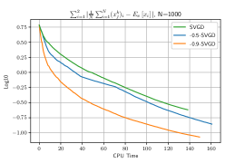
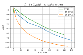
Figure 2: The target distribution is $\pi(x)=\frac{2}{5}\mathcal{N}((2,0),I_{2})+\frac{1}{5}\mathcal{N}((4,0),I_{2})+\frac{2}{5}\mathcal{N}((3,-3),I_{2})$. Each sampled point $x_{j}^{k}$ is of the form $\left((x_{j}^{k})_{1},(x_{j}^{k})_{2}\right)$, where $k$ denote the $k$-th iteration, $j$ denote the $j$-th sampled point. For distribution $\pi$, we have $\mathbb{E}_{\pi}\left[x_{1}\right]=2.8,\mathbb{E}_{\pi}\left[x_{2}\right]=-1.2$ and $\mathbb{E}_{\pi}\left[(x_{1})^{2}\right]=9.4,\mathbb{E}_{\pi}\left[(x_{2})^{2}\right]=4.6$. The initial $N$ points are sampled from $\mathcal{N}\left((-2,0),I_{2}\right)$. The step-size $\gamma$ for both algorithms equals $0.2$. In $\beta$-SVGD, we choose the small gap $\tau=0.01$ and we update the Stein importance weights every $20$ iterations using $40$ mirror descent steps with step-size $r=0.3$. Since the function computed in the second image is $x^{2}$, it is not surprising that there is an increase in the first few iterations.

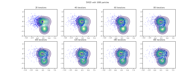
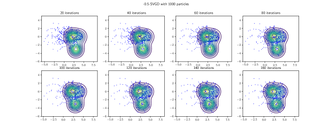
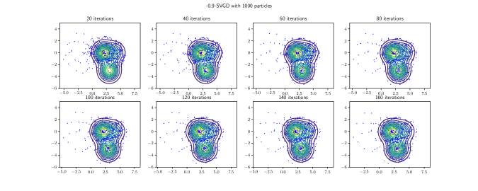
Figure 3: The same experiment setting as in Figure 1. We show how the particles move in the update of $\beta$-SVGD with $\beta=0,-0.5,-0.9$.

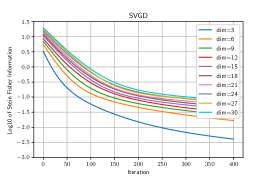
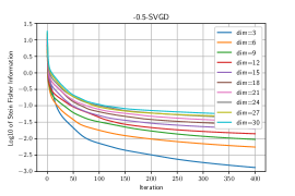
Figure 4: In this experiment, we show how the Stein Fisher information changes in the update of SVGD and $-0.5$-SVGD. The target distribution is $\mathcal{N}((2,\ldots,2)_{d},I_{d})$ and the initial points are sampled from $\mathcal{N}((0,\ldots,0)_{d},I_{d})$ with $N=300$. The step-size $\gamma=0.1$ for both algorithm and for $-0.5$-SVGD algorithm, we set the small gap $\tau=0.01$ and we update the Stein importance weight in every iteration using $40$ mirror descent with step-size $r=0.3$. We can see that the Stein Fisher information drops immediately below $1$ (note in the picture, the axis $y$ is $\log_{10}$ of the Stein Fisher information) in $-0.5$-SVGD, while in SVGD it drops slowly.

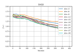
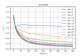
Figure 5: The experiment settings are the same as in Figure 4. We compare how the Stein importance weight changes in the update of SVGD and $-0.5$-SVGD (though we don’t have to compute the Stein importance weight in the implementation of SVGD). The error is defined by $f(\omega^{k}):=\sum_{i=1}^{N}|w_{i}^{k}-\frac{1}{N}|$, where $\omega_{i}^{k}$ denote the Stein importance weight of point $x_{i}^{k}$ and $N=300$. The results suggest that in high dimensional cases, the Stein importance weight can help to accelerate the decreasing of Stein Fisher information in the beginning, then it will approach to the identical weight $\frac{1}{N}$ quickly.

D.2 Bayesian Logistic Regression

In Figure 6, we compare the performance of SVGD and $\beta$-SVGD with $\beta=-0.5$ in Bayesian Logistic regression problem. This Bayesian Logistic regression experiment is done in Liu & Wang (2016) to compare SVGD with several Markov Chain Monte Carlo methods, more details about this experiment can refer to Liu & Wang (2016). As in the Gaussian Mixtures experiment, we choose the reproducing kernal $k(x,y)=e^{-\frac{\left\|x-y\right\|^{2}}{d}}$.

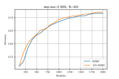
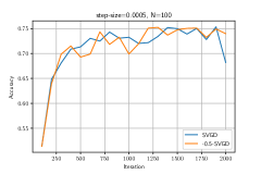
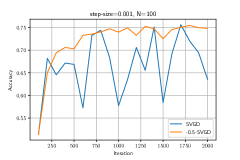
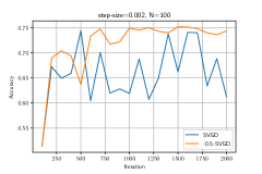
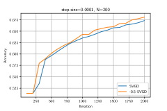
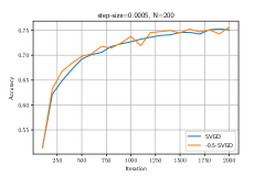
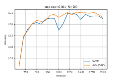
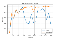
Figure 6: In this experiment, we test the binary Covertype dataset with 581,012 data points and 54 features ($d=54$). We run $2000$ iterations of SVGD and $\beta$-SVGD with different step-size and number of particles. In each iteration of $-0.5$-SVGD, we run $200$ steps of mirror descent with step-size $r=2$ (since the values of the entries of $\bm{K}_{\pi}$ in this experiment can be very big, we need to rescale the matrix by dividing a factor of $10^{9}$ to resolve the overflow problem, so the step-size for mirror descent is chosen relatively big) to find the Stein importance weights, we set the small gap $\tau=0.05$. The time required to run $2000$ iterations of $-0.5$-SVGD and test the accuracy every $100$ iterations is roughly double that required for SVGD. In this experiment, we found the Stein importance weight is close to the identical weight after only a few $\beta$-SVGD iterations with relatively big step-size (specifically, the percentage of weight $\omega_{i}$ such that $N\omega_{i}<0.1$ falls to $0$ after the first few iterations of $-0.5$-SVGD), so the acceleration effect is not very clear in this case. However, as shown in the first and fifth images, where the step-size is relatively small, we can see a faster improvement in accuracy in the first few hundreds iterations of $\beta$-SVGD. We can also see from the results that when $\gamma$ is relatively large, due to the Stein importance weight, $-0.5$-SVGD is much more stable than SVGD.

References

- Ambrosio et al. (2005) Luigi Ambrosio, Nicola Gigli, and Giuseppe Savaré. Gradient flows: in metric spaces and in the space of probability measures. Springer Science & Business Media, 2005.
- Arnold et al. (2001) Anton Arnold, Peter Markowich, Giuseppe Toscani, and Andreas Unterreiter. On convex Sobolev inequalities and the rate of convergence to equilibrium for Fokker-Planck type equations. 2001.
- Bakry et al. (2014) Dominique Bakry, Ivan Gentil, Michel Ledoux, et al. Analysis and geometry of Markov diffusion operators, volume 103. Springer, 2014.
- Berlinet & Thomas-Agnan (2011) Alain Berlinet and Christine Thomas-Agnan. Reproducing kernel Hilbert spaces in probability and statistics. Springer Science & Business Media, 2011.
- Betancourt (2017) Michael Betancourt. A conceptual introduction to Hamiltonian Monte Carlo. arXiv preprint arXiv:1701.02434, 2017.
- Cao et al. (2019) Yu Cao, Jianfeng Lu, and Yulong Lu. Exponential decay of Rényi divergence under Fokker–Planck equations. Journal of Statistical Physics, 176(5):1172–1184, 2019.
- Cheng et al. (2018) Xiang Cheng, Niladri S Chatterji, Peter L Bartlett, and Michael I Jordan. Underdamped Langevin MCMC: A non-asymptotic analysis. In Conference on learning theory, pp. 300–323. PMLR, 2018.
- Dalalyan & Karagulyan (2019) Arnak S Dalalyan and Avetik Karagulyan. User-friendly guarantees for the Langevin Monte Carlo with inaccurate gradient. Stochastic Processes and their Applications, 129(12):5278–5311, 2019.
- Detommaso et al. (2018) Gianluca Detommaso, Tiangang Cui, Youssef Marzouk, Alessio Spantini, and Robert Scheichl. A Stein variational Newton method. Advances in Neural Information Processing Systems, 31, 2018.
- Duane et al. (1987) Simon Duane, Anthony D Kennedy, Brian J Pendleton, and Duncan Roweth. Hybrid Monte Carlo. Physics letters B, 195(2):216–222, 1987.
- Duncan et al. (2019) Andrew Duncan, Nikolas Nüsken, and Lukasz Szpruch. On the geometry of Stein variational gradient descent. arXiv preprint arXiv:1912.00894, 2019.
- Durmus & Moulines (2017) Alain Durmus and Eric Moulines. Nonasymptotic convergence analysis for the unadjusted Langevin algorithm. The Annals of Applied Probability, 27(3):1551–1587, 2017.
- Garbuno-Inigo et al. (2020) Alfredo Garbuno-Inigo, Franca Hoffmann, Wuchen Li, and Andrew M Stuart. Interacting Langevin diffusions: gradient structure and ensemble Kalman sampler. SIAM Journal on Applied Dynamical Systems, 19(1):412–441, 2020.
- Gorham & Mackey (2017) Jackson Gorham and Lester Mackey. Measuring sample quality with kernels. In International Conference on Machine Learning, pp. 1292–1301. PMLR, 2017.
- Gorham et al. (2020) Jackson Gorham, Anant Raj, and Lester Mackey. Stochastic Stein discrepancies. Advances in Neural Information Processing Systems, 33:17931–17942, 2020.
- Han & Liu (2017) Jun Han and Qiang Liu. Stein variational adaptive importance sampling. arXiv preprint arXiv:1704.05201, 2017.
- Kassab & Simeone (2022) Rahif Kassab and Osvaldo Simeone. Federated generalized Bayesian learning via distributed Stein variational gradient descent. IEEE Transactions on Signal Processing, 2022.
- Korba et al. (2020) Anna Korba, Adil Salim, Michael Arbel, Giulia Luise, and Arthur Gretton. A non-asymptotic analysis for Stein variational gradient descent. Advances in Neural Information Processing Systems, 33:4672–4682, 2020.
- Li et al. (2020) Lei Li, Yingzhou Li, Jian-Guo Liu, Zibu Liu, and Jianfeng Lu. A stochastic version of Stein variational gradient descent for efficient sampling. Communications in Applied Mathematics and Computational Science, 15(1):37–63, 2020.
- Li & Ying (2019) Wuchen Li and Lexing Ying. Hessian transport gradient flows. Research in the Mathematical Sciences, 6(4):1–20, 2019.
- Liu (2017) Qiang Liu. Stein variational gradient descent as gradient flow. Advances in Neural Information Processing Systems, 30, 2017.
- Liu & Lee (2017) Qiang Liu and Jason Lee. Black-box importance sampling. In Artificial Intelligence and Statistics, pp. 952–961. PMLR, 2017.
- Liu & Wang (2016) Qiang Liu and Dilin Wang. Stein variational gradient descent: A general purpose bayesian inference algorithm. Advances in Neural Information Processing Systems, 29, 2016.
- Liu et al. (2017) Yang Liu, Prajit Ramachandran, Qiang Liu, and Jian Peng. Stein variational policy gradient. arXiv preprint arXiv:1704.02399, 2017.
- Mansour et al. (2012) Yishay Mansour, Mehryar Mohri, and Afshin Rostamizadeh. Multiple source adaptation and the Rényi divergence. arXiv preprint arXiv:1205.2628, 2012.
- Morales González et al. (2013) Domingo Morales González, Leandro Pardo Llorente, and Igor Vadja. Rényi statistics in directed families of exponential experiments. Ene, 9:30, 2013.
- Neal (2011) R. M Neal. MCMC using Hamiltonian dynamics. Handbook of Markov Chain Monte Carlo, 2(11):2, 2011.
- Pu et al. (2017) Yuchen Pu, Zhe Gan, Ricardo Henao, Chunyuan Li, Shaobo Han, and Lawrence Carin. VAE learning via Stein variational gradient descent. Advances in Neural Information Processing Systems, 30, 2017.
- Salim et al. (2021) Adil Salim, Lukang Sun, and Peter Richtárik. Complexity analysis of Stein variational gradient descent under Talagrand’s inequality T1. arXiv preprint arXiv:2106.03076, 2021.
- Shi et al. (2021) Jiaxin Shi, Chang Liu, and Lester Mackey. Sampling with mirrored Stein operators. arXiv preprint arXiv:2106.12506, 2021.
- Silverman (2018) Bernard W Silverman. Density estimation for statistics and data analysis. Routledge, 2018.
- Sun et al. (2022) Lukang Sun, Avetik Karagulyan, and Peter Richtárik. Convergence of Stein variational gradient descent under a weaker smoothness condition. arXiv preprint arXiv:2206.00508, 2022.
- Tao et al. (2019) Chenyang Tao, Shuyang Dai, Liqun Chen, Ke Bai, Junya Chen, Chang Liu, Ruiyi Zhang, Georgiy Bobashev, and Lawrence Carin. Variational annealing of GANs: A Langevin perspective. In International Conference on Machine Learning, pp. 6176–6185. PMLR, 2019.
- Van Erven & Harremos (2014) Tim Van Erven and Peter Harremos. Rényi divergence and Kullback-Leibler divergence. IEEE Transactions on Information Theory, 60(7):3797–3820, 2014.
- Villani (2009) Cédric Villani. Optimal transport: old and new, volume 338. Springer, 2009.
- Wang et al. (2018) Dilin Wang, Hao Liu, and Qiang Liu. Variational inference with tail-adaptive f-divergence. Advances in Neural Information Processing Systems, 31, 2018.
- Wang et al. (2019) Dilin Wang, Ziyang Tang, Chandrajit Bajaj, and Qiang Liu. Stein variational gradient descent with matrix-valued kernels. Advances in Neural Information Processing Systems, 32, 2019.
- Yu et al. (2020) Lantao Yu, Yang Song, Jiaming Song, and Stefano Ermon. Training deep energy-based models with f-divergence minimization. In International Conference on Machine Learning, pp. 10957–10967. PMLR, 2020.
- Zhang et al. (2018) Ruiyi Zhang, Chunyuan Li, Changyou Chen, and Lawrence Carin. Learning structural weight uncertainty for sequential decision-making. In International Conference on Artificial Intelligence and Statistics, pp. 1137–1146. PMLR, 2018.
- Zhang et al. (2019) Ruiyi Zhang, Zheng Wen, Changyou Chen, and Lawrence Carin. Scalable Thompson sampling via optimal transport. arXiv preprint arXiv:1902.07239, 2019.