An In-depth Study of Stochastic Backpropagation

Abstract

In this paper, we provide an in-depth study of Stochastic Backpropagation (SBP) when training deep neural networks for standard image classification and object detection tasks. During backward propagation, SBP calculates the gradients by only using a subset of feature maps to save the GPU memory and computational cost. We interpret SBP as an efficient way to implement stochastic gradient decent by performing backpropagation dropout, which leads to considerable memory saving and training process speedup, with a minimal impact on the overall model accuracy. We offer some good practices to apply SBP in training image recognition models, which can be adopted in learning a wide range of deep neural networks. Experiments on image classification and object detection show that SBP can save up to 40% of GPU memory with less than 1% accuracy degradation.

1 Introduction

A common practice to improve accuracy when training deep neural networks is to increase the input resolution [19], model depth [7], and model width [21]. However, this can significantly increase the GPU memory usage, making training on devices with limited resources difficult. For example, when training an object detector using ConvNeXt-Base [14] as the backbone with batch size 2, requires over 17 GB of memory, which cannot fit on most modern GPUs.

Many prior studies have focused on designing memory-efficient training method, especially for large model training on high resolution images or videos. Mixed-precision training [17] uses lower precision to represent the network weights and activations for certain layers of the network. Gradient checkpointing [2] restores intermediate feature maps by recomputing nodes in the computation graph during the backward pass, which requires extra computations. Gradient accumulation [12] splits a mini-batch into smaller chunks to calculate gradients iteratively, which slows down training process.

A recent method, Stochastic Backpropagation (SBP) [3], offers a new perspective for memory-efficient model training. It performs partial execution of gradients during backpropagation on randomly selected frames when training video models [13, 24, 23, 22]. It achieves considerable memory saving by only caching a subset of video frame feature maps without significant accuracy loss. However, SBP in [3] is only applied to video-based models using two architectures and its design space has not be thoroughly explored to wider tasks. The explanation provided in [3] for the effectiveness of SBP is simple but narrow — it attributes the validity of the method to the high redundancy of video.

This leaves many questions around SBP unanswered: (1) Is SBP’s effectiveness limited to operating on the redundancy of video frames or can it effectively leverage spatial redundancy? (2) If so, can SBP be generalized to image-based tasks, with more limited redundancy? (3) Is SBP generalizable to different networks (e.g., MLP, CNN, Transformer) and operators? (4) What are the key design choices when implementing SBP?

To answer these questions, we first formalize the SBP process in a general form and analyze the effect of SBP on the calculation of gradients. With this formulation, we show how to generalize the idea of SBPto image models and present an in-depth study of the design choices when using SBP. During backward propagation, SBP calculates gradients from a subset of spatial feature maps to save memory and computation cost. We observe that the calculated gradients by SBP are highly correlated with the standard SGD gradients, indicating SBP is a reasonable approximation. We also provide a new, straightforward implementation of the idea that requires only a few lines of code. We explore several important design strategies which have a noticeable impact on the performance. We validate the generalizability of SBP on two common tasks (image classification and object detection) with two popular network architectures: ViT [6] and ConvNeXt [14]. We show that SBP can effectively train image models with less than 1% loss of accuracy in a memory-efficient fashion.

2 Related Work

Since deep neural networks are highly extended in both depth [7] and breadth [21] in recent years, designing memory-efficient training methods has attracted a fair amount of attention. By saving and recomputing nodes in the computation graph during backpropagation, gradient checkpointing [2] can save a large amount of memory. Besides, gradient accumulation [12] splits the large sample batch into several mini batches and runs them iteratively without updating model parameters. This saves the GPU memory proportionally without affecting the accuracy, because accumulating the gradients of these sub-iterations and then updating the model parameters is identical to directly optimizing the model with a global batch size. However, these two methods slow down the training process. Multigrid [20] proposes to use different mini-batch shapes to speedup the model training. Sparse network [5] particularly targets the recognition tasks but can only save the memory theoretically. Sideways [15] and its follow-up [16] reduce the memory cost by overwriting activations whenever new ones become available, but they are limited to causal models. SBP [3] reduces a large portion of GPU memory by only backpropagating gradients from incomplete execution for video models. In this paper, we generalize SBP to more standard computer vision tasks including image recognition.

3 Understanding Stochastic Backpropagation (SBP)

In this section, we first formalize the process of Stochastic Backpropagation (SBP) (sec. 3.1) and show how to compute the gradient for two common operations (sec. 3.2). With these formulations established, we analyze how to perform the chain rule of gradient calculations for SBP (sec. 3.3). Finally, we present a simple implementation of SBP in practice with only a few lines of code (sec. 3.4).

3.1 Formulation of SBP

We first present a general formulation of SBP [3]. We denote a loss function $L(\Theta)$ to learn a model on a dataset $D=\{d_{j}\}_{j=1}^{N}$, where $\Theta$ is the collection (vector, matrix, or tensor) of all parameters of the model, $N$ is the total number of training samples, $d_{j}\in\mathbb{R}^{T\times H\times W\times C}$ is an input data sample, where $H$ and $W$ are spatial resolution height and width respectively, $C$ is the input channel size, $T=1$ represents an image and $T>1$ represents a video.

In each training iteration, the model with SBP processes a mini-batch of data samples $S\in\mathbb{R}^{B\times T\times H\times W\times C}\subseteq D$ to compute the loss in the forward pass, where $B$ is the batch size. During the backward pass, different from the traditional backpropagation that relies on the full feature maps $X_{i}\in\mathbb{R}^{B\times T_{i}\times H_{i}\times W_{i}\times C_{i}}$($i$ is the index of the layers), an incomplete execution for backpropagation (i.e., SBP) only utilizes a subset of the feature maps $X_{i}^{sub}\in\mathbb{R}^{B\times T_{i}^{sub}\times H_{i}^{sub}\times W_{i}^{sub}\times C_{i}}$ to approximate the gradient calculation. That is, it updates the model weights as

$$\Theta_{iter+1}=\Theta_{iter}-\eta\frac{1}{B}\sum_{x_{i}^{sub}\in X_{i}^{sub}}\nabla_{\Theta}L(x_{i}^{sub},\Theta_{iter}),$$ (1)

where $\eta$ is the learning rate, $\nabla_{\Theta}$ is the collection of model weight gradients, $\Theta_{iter}$ and $\Theta_{iter+1}$ are model weights at the current and next iteration, respectively.

SBP saves memory by only caching a subset of feature maps in the backward pass, but it keeps all the full forward paths. Note that the method in [3] is a special case of (1) as it performs on the temporal dimension and uses a subset of video frames $X_{i}^{T_{i}^{sub}}\in\mathbb{R}^{B\times T_{i}^{sub}\times H_{i}\times W_{i}\times C_{i}}$.

3.2 Backward Gradient Calculation

Next, we derive equations to compute the gradient during the backward phase of SBP. We denote that at layer $i$ of the model, an operator $f_{i}$ with learnable weights $W_{f_{i}}$ to processes the feature maps $X_{i}\in\mathbb{R}^{B\times T_{i}\times H_{i}\times W_{i}\times C_{i}^{in}}$, where $C_{i}^{in}$ refers to the input channel size.

3.2.1 Calculation of Linear Layers

We start with exploring $f_{i}$ as a point-wise convolutional (PW-Conv) layer. PW-Conv is widely used in the state-of-the-art computer vision models such as ViT [6] and ConvNeXt [14]. It is equivalent to the linear layers in Transformer MLP blocks [14], and is also known as channel-wise fully connected layer. It can be either implemented through the linear layer, or the $1\times 1$ convolutional layer. It is mainly used to enrich the channel information with weights $W_{f_{i}}\in\mathbb{R}^{C_{i}^{in}\times C_{i}^{out}}$, and the analysis on PW-Conv can be easily extended to other layers.

The forward pass of this layer is (the bias term is omitted):

$$X_{i+1}=f_{i}(X_{i})=X_{i}W_{f_{i}},$$ (2)

where $X_{i+1}\in\mathbb{R}^{(B\times T_{i}\times H_{i}\times W_{i})\times C_{i}^{out}}$ ($X_{i}$ and $X_{i+1}$ are reshaped as a matrix format). During the traditional backward pass with full backpropagation, the gradients of both activations and weights are calculated by:

$$\begin{array}[]{ll}dX_{i+1}&=\partial Loss/\partial X_{i+1},\vspace{1mm}\\ dW_{f_{i}}&=\partial Loss/\partial W_{f_{i}}=X_{i}^{T}dX_{i+1},\vspace{1mm}\\ dX_{i}&=\partial Loss/\partial X_{i}=dX_{i+1}W_{f_{i}}^{T}.\end{array}$$ (3)

It requires storing the weights $W_{f_{i}}\in\mathbb{R}^{C_{i}^{in}\times C_{i}^{out}}$ and full feature maps $X_{i}\in\mathbb{R}^{(B\times T_{i}\times H_{i}\times W_{i})\times C_{i}^{in}}$ to compute the gradients. In many cases, $B\times T_{i}\times H_{i}\times W_{i}\gg C_{i}^{out}$, i.e., caching of feature maps dominates the memory usage. In order to effectively save GPU memory during training, SBP only caches a subset of the feature maps for backpropagation.

In the backward pass of SBP process, we split the full feature maps $X_{i}$ into two subsets $X_{i}^{keep}$ and $X_{i}^{drop}$, which denote the corresponding indices of the sampled feature maps that are kept and dropped, respectively. An example of $X_{i}^{keep}$ can be $X_{i}[:,\mbox{even index on }T,:,:,:]$ for video, or $X_{i}[:,:,\mbox{even index on }H,\mbox{odd index on }W,:]$ for image (e.g., Fig. 3 left), and $X_{i}^{drop}$ is the complementary part of the feature maps. We have $X_{i}^{keep}\cap X_{i}^{drop}=\emptyset$ and $X_{i}^{keep}\cup X_{i}^{drop}=X_{i}$. We denote keep-ratio $r$ as the number of gradient kept indices $j\in\mathbb{Z}_{i}^{keep}$ over the number of all indices.

One advantage of simplifying the SBP problem by using PW-Conv operator is that the nodes in spatial or temporal dimensions can be calculated independently through the forward and backward passes. Therefore, we can update the forward pass separately on the kept and dropped indices:

$$\begin{array}[]{ll}&X_{i+1}=[X_{i+1}^{keep},X_{i+1}^{drop}]=[X_{i}^{keep},X_{i}^{drop}]W_{f_{i}},\vspace{1mm}\\ &\mbox{i.e.,}\quad X_{i+1}^{keep}=X_{i}^{keep}W_{f_{i}},\quad X_{i+1}^{drop}=X_{i}^{drop}W_{f_{i}}\end{array}$$ (4)

as well as the backward pass:

$$\begin{array}[]{ll}&dX_{i+1}=[dX_{i+1}^{keep},dX_{i+1}^{drop}],\vspace{1.5mm}\\ &dX_{i}^{keep}=dX_{i+1}^{keep}W_{f_{i}}^{T},\quad dX_{i}^{drop}=dX_{i+1}^{drop}W_{f_{i}}^{T},\vspace{1.5mm}\\ &dW_{f_{i}}=X_{i}^{T}dX_{i+1}=[X_{i}^{keep},X_{i}^{drop}]^{T}[dX_{i+1}^{keep},dX_{i+1}^{drop}]\vspace{1.5mm}\\ &={X_{i}^{keep}}^{T}dX_{i+1}^{keep}+{X_{i}^{drop}}^{T}dX_{i+1}^{drop}.\end{array}$$ (5)

SBP drops all the gradients calculation with superscripts ^drop and keeps all the gradients calculation with superscripts ^keep, thus it saves memory and computation on the dependencies of dropped indices. In other words, the memory usage and the backward computation cost is proportional to the keep-ratio of the original case. Mathematically, it is equivalent to set $dX_{i+1}^{drop}=\textbf{0}$ (thus $dX_{i}^{drop}=\textbf{0}$) and uses $dW_{f_{i}}^{keep}={X_{i}^{keep}}^{T}dX_{i+1}^{keep}$ as a stochastic approximation of the original weight gradients $dW_{f_{i}}$ to update the model weights.

3.2.2 Calculation of Convolutional Layers

We then derive the calculation of a general convolutional layer (ConvLayer) as $f_{i}$. Unlike the PW-Conv, nodes of general ConvLayer with kernel size $>1$ in spatial or temporal dimensions are no longer independent in forward and backward calculations. Assume that we apply a convolutional kernel $k\times k$ with stride $s$. The regular backpropagation of the ConvLayer is calculated as follows:

$$\begin{array}[]{ll}&dX_{i}=zeropad(dX_{i+1})\ast W_{f_{i}}^{\prime}\vspace{1mm}\\ &dW_{f_{i}}=X_{i}\ast dX_{i+1}\end{array}$$ (6)

where $\ast$ is the convolution operation, $zeropad$ is to pad the edge of the matrix with zeros, and $W_{f_{i}}^{\prime}$ represents the $180^{\circ}$ rotation of $W_{f_{i}}$.

From Eq. (6), in the gradient calculation of ConvLayer at a given location $j$ on the input feature map as $x_{i}^{j}\in X_{i}$, all the elements from $dX_{i+1}$ inside the region of the kernel size $k$ will contribute to the gradient calculation of $dx_{i}^{j}$. Therefore, in SBP of ConvLayer, when we set $dX_{i+1}^{drop}=\textbf{0}$ for certain areas, in general, two things will happen: (a) even if $j\in\mathbb{Z}^{drop}$ and $dx_{i+1}^{j}=0$, $dx_{i}^{j}$ will not be $0$ due to the non-zero gradient contribution of the neighbors of $j$ on $dX_{i+1}$; (b) $dx_{i}^{j}$ will be an approximated gradient unless all $dx_{i+1}^{p}$ with $p$ in the neighbor areas of $j$ in terms of the kernel size $k$ (i.e., indices $p$ are within the convolutional kernel of index $j$) are kept and there is no chain rule effect on $dx_{i+1}^{p}$. However, there is a special scenario: when $s\geq k$, the neighbor effects disappear due to the fact that $dX_{i+1}$ needs to be zero interweaved in gradient calculation. As a result, nodes in spatial or temporal dimensions are getting more independent, which is similar to the case of PW-Conv.

3.2.3 Discussion

From the derivation above, we see that the approximation effect of SBP performs differently when the operator changes. For layers such as linear layer or PW-Conv, the activation gradients (i.e., $dx_{i}$) are either 0 or exact. While for convolutional layers with kernel size larger than 1, most of the gradients on the activations are neither 0 nor exact. Due to space limitation, we only derived SBP on two most popular operators. For derivation of other operators, please refer to the supplementary material.

3.3 Chain Rule Effect

We have derived the calculation of SBP on a single layer in the previous section. In this section, we derive the calculation of SBP on a stack of multiple layers. For simplicity, we take two layers as an example, which can be easily generalized to more layers.

3.3.1 Two PW-Conv Layers

We first consider a scenario with two PW-Conv layers. We assume a layer before $f_{i}$, i.e., $f_{i-1}$, is another PW-Conv layer with weights $W_{f_{i-1}}$. The forward pass of this layer is (the bias term is also omitted):

$$X_{i}=f_{i-1}(X_{i-1})=X_{i-1}W_{f_{i-1}}.$$ (7)

Then we can calculate the gradients of weights and activations in layer $f_{i-1}$ similar to Eq. (3):

$$\begin{array}[]{ll}&dX_{i-1}=dX_{i}W_{f_{i-1}}^{T}=dX_{i+1}W_{f_{i}}^{T}W_{f_{i-1}}^{T},\vspace{1.5mm}\\ &dW_{f_{i-1}}=X_{i-1}^{T}dX_{i}=X_{i-1}^{T}dX_{i+1}W_{f_{i}}^{T}.\end{array}$$ (8)

We first consider the case when there is no additional gradient dropout at layer $f_{i-1}$. Since $dX_{i+1}$ has non-zero gradients at kept indices (i.e., $dX_{i+1}^{keep}$) and zero gradients at dropped indices (i.e., $dX_{i+1}^{drop}$), Eq. (8) can be updated to:

$$\begin{array}[]{ll}&dX_{i-1}=[dX_{i-1}^{keep},dX_{i-1}^{drop}],\vspace{1.5mm}\\ &dX_{i-1}^{keep}=dX_{i+1}^{keep}W_{f_{i}}^{T}W_{f_{i-1}}^{T},\quad dX_{i-1}^{drop}=dX_{i+1}^{drop}W_{f_{i}}^{T}W_{f_{i-1}}^{T}=\textbf{0},\vspace{1.5mm}\\ &dW_{f_{i-1}}={X_{i-1}^{keep}}^{T}dX_{i+1}^{keep}W_{f_{i}}^{T}.\end{array}$$ (9)

From the equation, we can see that if there is no additional gradient dropout applied on layer $f_{i-1}$, through the chain rule, the keep and drop set will transfer from $X_{i+1}$ to $X_{i-1}$ identically.

If we apply gradient dropout on layer $f_{i-1}$ as well, i.e., on layer $f_{i-1}$, we split $dX_{i}$ into $dX_{i}^{keep}$ and $dX_{i}^{drop}$. Assume that the keep and drop indices set at layer $i+1$ is $\mathbb{Z}_{i+1}^{keep}$ and $\mathbb{Z}_{i+1}^{drop}$, and at layer $i$ is $\mathbb{Z}_{i}^{keep}$ and $\mathbb{Z}_{i}^{drop}$, respectively. Then through Eq. (8) and Eq. (9), the keep and drop indices set on layer $i-1$ will be:

$$\small\mathbb{Z}_{i-1}^{keep}=\mathbb{Z}_{i+1}^{keep}\cap\mathbb{Z}_{i}^{keep},\quad\mathbb{Z}_{i-1}^{drop}=\mathbb{Z}_{i+1}^{drop}\cup\mathbb{Z}_{i}^{drop}.$$ (10)

Eq. (9) becomes:

$$\begin{array}[]{ll}&dX_{i-1}=[dX_{i-1}^{keep^{\prime}},dX_{i-1}^{drop^{\prime}}],\vspace{1.5mm}\\ &dX_{i-1}^{keep^{\prime}}=dX_{i+1}^{keep^{\prime}}W_{f_{i}}^{T}W_{f_{i-1}}^{T},\quad dX_{i-1}^{drop^{\prime}}=\textbf{0},\vspace{1.5mm}\\ &dW_{f_{i-1}}={X_{i-1}^{keep^{\prime}}}^{T}dX_{i+1}^{keep^{\prime}}W_{f_{i}}^{T}.\end{array}$$ (11)

where $keep^{\prime}=\mathbb{Z}_{i-1}^{keep}$ and $drop^{\prime}=\mathbb{Z}_{i-1}^{drop}$.

3.3.2 PW-Conv + ConvLayers

Now let’s look at the chain-rule effect of the case when $f_{i-1}$ is a ConvLayer with kernel size $k>1$ and stride $s$. Using the chain rule, we can update the Eq. (6) as follows:

$$\begin{array}[]{ll}&dX_{i-1}=zeropad(dX_{i})\ast W_{f_{i-1}}^{\prime}=zeropad(dX_{i+1}W_{f_{i}}^{T})\ast W_{f_{i-1}}^{\prime},\vspace{1.5mm}\\ &dW_{f_{i-1}}=X_{i-1}\ast dX_{i}=X_{i-1}\ast dX_{i+1}W_{f_{i}}^{T}.\end{array}$$ (12)

We can see from above equation that each $dx_{i-1}^{j}$ receives the backward gradients from the neighbors of $dx_{i}^{j}$, which might be partially dropped out, thus the gradient at $dx_{i-1}^{j}$ is no longer exact.

From Eq. (12), the dropout at layer $i$ makes the matrix $dX_{i}$ sparse (only indices at $\mathbb{Z}_{i+1}^{keep}$ are non-zero). If we conduct dropout at the current layer $f_{i-1}$ (i.e., we have $\mathbb{Z}_{i}^{keep}$ and $\mathbb{Z}_{i}^{drop}$), the matrix $dX_{i-1}$ will become even more sparse unless the dropout is happening on the same location $\mathbb{Z}_{i+1}^{drop}=\mathbb{Z}_{i}^{drop}$. If we stack PW-Conv + ConvLayer further and further in an interweaving way (i.e., $\mathbb{Z}_{i+1}^{drop}\neq\mathbb{Z}_{i}^{drop}$), the chain rule effect may lead to a very sparse output derivative matrix (e.g., $dX_{i-1}$). However, stacking ConvLayers (due to the space limitation, we skip the math derivation) will not have such a trend, as the gradient dropout in ConvLayer only creates approximated gradient but not many zeros, because of the neighbor effect of gradient calculation.

3.3.3 Discussion

Overall, in terms of the chain rule effect, we can see from Eq. (11) that stacking PW-Conv layers, especially in an interweaving way may lead to a sparse keep set $\mathbb{Z}_{i-1}^{keep}$ and a vanishing gradient of $dW_{f_{i-1}}$. However, in practice, we always drop gradients at the same positions across layers to avoid the gradient vanishing problem and to achieve good accuracy performance. Stacking PW-Conv + ConvLayers (in Eq. (12)) also tends to make the keep set sparse. While stacking ConvLayers doesn’t have such effect, though it stacks the non-exact gradient at almost every position and tends to make the gradients gradually move away from the original ones.

3.4 Efficient Implementation

With a deeper understanding of how SBP works, we provide a simple and efficient implementation of the SBP technique in Alg. 1. We point out that this is more efficient than the prior work [3] as there is (1) no need to do the re-forward in the backward, thus it is computationally more efficient, and (2) no need to manually cache the intermediate feature maps and fill zero gradients in the backward, which is much simpler. We emphasize that it is very simple and easy to implement, it only needs 3 lines of code to do the forward, and the backward (no need to implement manually) can be seamlessly handled by the ease of “autograd engine” in the deep learning frameworks. It supports point-wise convolutional layers, the dot-product attention layers, and multilayer perception (MLP) in popular networks including ViT [6] and its variants [6, 11, 13], ConvNeXt [14], and hybrid architectures [4].

Algorithm 1 Pytorch-like pseudocode of SBP for an arbitrary operation $f$.

⬇

# f: an arbitrary operation

# grad_keep_idx: sampled indices where gradients are kept

# grad_drop_idx: sampled indices where gradients are dropped

def sbp_f(f, inputs, grad_keep_idx, grad_drop_idx):

# initiate outputs

outputs = torch.zeros(output_shape, device=inputs.device)

# forward with gradient calculation, gradients will be calculated with torch.autograd

with torch.enable_grad():

outputs[grad_keep_idx] = f(inputs[grad_keep_idx])

# forward without gradient calculation

with torch.no_grad():

outputs[grad_drop_idx] = f(inputs[grad_drop_idx])

return outputs

 

4 Design Strategies

In this section, we investigate the effectiveness of different design strategies of SBP on image tasks. We use ViT-Tiny [6] model to evaluate the top-1 accuracy on ImageNet [18] validation dataset. The ViT-Tiny is a smaller version of the ViT [6] variants, it uses patch size $16$ with 12 transformer blocks (more than 80 layers), the embedding dimension is 192 and the number of heads is 3, i.e., each head has dimension 64. The experiments are trained for 100 epochs on the ImageNet training dataset. The conclusions remain for larger models and more training epochs.

How many layers should be applied with SBP? To answer this question, we progressively apply SBP to transformer layers from the last layers to early layers and present their results in Fig. 2 Left. As shown, we observe a sweet spot when applying SBP to 8 out of 12 block layers, which saves 33% of GPU memory with an accuracy drop within 1.5%. Although applying SBP on all the transformer layers can save the most GPU memory, it causes a large accuracy drop. Therefore, unless stated otherwise, we apply SBP on 2/3 of all layers of ViT models for the rest of this work.

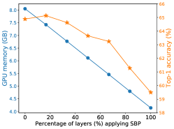
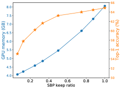
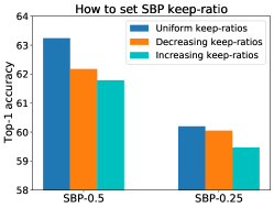
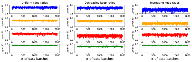
Figure 1: Illustration of the effect on applying SBP on different choices of the network layers and keep-ratios. Left: accuracy curve of applying SBP on different percentage of layers, the keep ratio of SBP is 0.5. Middle: trade-off of keep-ratio versus accuracy, every SBP layer has the same keep-ratio. Right: comparison of using uniform, decreasing and increasing keep-ratios for the SBP layers.

Figure 2: Cosine similarity of weights gradient between with and without applying SBP on ViT-Tiny with uniform, decreasing, and increasing keep-ratios. Results on Layer 20 (MHSA), 40 (MLP), 60 (LayerNorm), 80 (MLP) are displayed. Results on other layers have similar behavior.

How much gradients should be kept in SBP? In this section, we discuss the trade-off between the gradients keep-ratio and accuracy in SBP. As a reminder, keep-ratio $r$ is the number of gradients kept indices over the number of all indices, and it represents the percentage of spatial feature map values used to calculate the gradients. In general, the higher the keep-ratio is, the more gradient information is preserved, and the higher the accuracy is, but the less memory is saved. A natural question arises: what is a good keep-ratio to balance the accuracy drop and memory saving?

In Fig. 2 Middle, we show the trade-off between model accuracy and the keep-ratio of gradients. In this case, we apply the same keep-ratio to all the SBP layers at the same gradient kept indices and we call it uniform keep-ratios method. We observe that setting the keep-ratio to be 0.5 is a golden rule, and having a keep-ratio of 0.25 is too aggressive, which results in a dramatic accuracy drop (3.04%) of the model. We also explore different keep-ratio methods by linearly increasing or decreasing the keep-ratios from early to late layers while keeping their average keep-ratio to be 0.5. Specifically, the keep-ratios are $[0.25,0.32,0.39,0.46,0.53,0.60,0.68,0.75]$ (increasing) or its inverse (decreasing) on 8 transformer blocks. As shown in Fig. 2 Right, both models perform significantly worse.

We simulate the gradient calculation on ViT-Tiny with 2000 data batches randomly sampled from the ImageNet training dataset. We apply different keep-ratio methods on the same model with the same fixed weights, and calculate the correlation (measured by cosine similarity) between the weights gradient of applying SBP and the original exact weights gradient without applying SBP, i.e., $Cosine(dW_{{}_{SBP}},dW_{{}_{no-SBP}})$. From Fig. 2, we observe that the weights gradient has a stronger correlation by using uniform keep-ratios compared to increasing or decreasing keep-ratios. We believe that uniform keep-ratios can keep the consistency of gradient dropping locations between different layers and can preserve gradient information at these spatial locations. However, non-uniform keep-ratios will have different dropping locations between different layers. As an overall result, it may lose more gradient information on more spatial locations and produce a less accurate estimation of the original gradients, and hence it may have a lower accuracy performance.

How to sample the gradient keep mask? SBP calculates the gradients by only using a subset of feature maps. A key question is how to sample the subset of feature maps to mask the kept gradients. If we fix the spatial locations of the gradient kept indices for every training step, the backward only propagates the valid gradients (non-zeros) on these fixed locations, which forces the model to only learn from fixed partial spatial information and therefore severely hurts the model performance. A better strategy is to randomly sample the gradient kept indices in each training step, so that it can statistically visit every spatial location with equal importance.

We examine two mask sampling strategies: grid-wise mask sampling and random mask sampling. See Fig. 3 left as a particular example of keep-ratio 0.5. We report the accuracy in Fig. 4 left. Overall, grid-wise mask sampling achieves $0.5\%\sim 1.7\%$ higher accuracy over random mask sampling. In Fig. 3, a stronger correlation is also observed by using the grid-wise sampling. One explanation is that grid-wise sampling is a more structured sampling method and it provides a more accurate estimation of gradients calculation. Unless stated otherwise, we use grid-wise sampling in this paper.

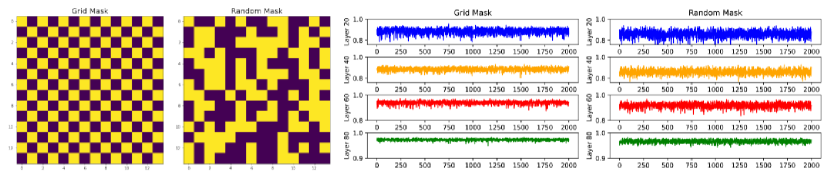
Figure 3: Left two: a particular example of gradient keep mask for grid-wise sampling and random sampling. Right two: cosine similarity of weights gradient between with and without applying SBP on ViT-Tiny. The SBP are applied with a keep-ratio of 0.5 on these two mask sampling methods.

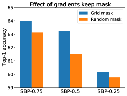
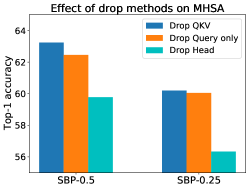
Figure 4: Left: effect of different sampling method for gradient keep mask. Right: effect of different SBP dropping methods on Multi-Head Self-Attention (MHSA).

How to apply SBP on MHSA? In general, the transformer block consists of two sub-blocks: Multi-Head Self-Attention (MHSA) and Multi-Layer Perception (MLP). Theoretically, the memory usage of applying SBP on MLP (two linear layers) is proportional to the keep-ratio $r$. However, the memory saving of applying SBP on MHSA depends on the sampling method on the query, key, value (QKV), and the ratio of head dimension $d$ over the number of tokens $n$. From [3], activation maps needed for gradients calculation in MHSA include the inputs and outputs ($2hdn$), QKV vectors (each with $hdn$), the attention weight maps ($2hnn$ before and after the softmax), thus requiring the memory of $3hdn+2hnn$ in total, where $h$ is the number of heads. Dropping gradients on query only (Drop Query only) or on all QKV (Drop QKV) enjoys the following memory usage ratio:

$$\small\begin{array}[]{ll}&\mbox{Drop Query only:}\quad\frac{2hdn+hdnr+2hnnr}{3hdn+2hnn}=\frac{r(\frac{d}{n}+2)+2\frac{d}{n}}{(\frac{d}{n}+2)+2\frac{d}{n}}\vspace{0.5mm}\\ &\mbox{Drop QKV:}\quad\frac{3hdnr+2hnnr^{2}}{3hdn+2hnn}=r\frac{3+2r\frac{d}{n}}{3+2\frac{d}{n}}\end{array}$$ (13)

In video transformers, the number of tokens $n$ is much larger than the head dimension $d$ (i.e., in video Swin Transformer [13] , $n=392$ and $d=32$, $\frac{d}{n}=0.082$) and thus the attention weight maps $2hnn$ comprise most of the memory. Therefore, dropping gradients on query only in the video model is good enough to save memory so that its memory is linearly proportional to the keep ratio $r$ [3].

However, in image task models such as ViT with a typical input size 224 and patch size 16, $n=14\times 14=196$ and $d=64$, $\frac{d}{n}=0.327$. With keep-ratio $r=0.5$ (or $r=0.25$), dropping gradients on query alone uses $0.61\times$ (or $0.42\times$) memory while dropping all QKV reduces its memory usage ratio to $0.46\times$ (or $0.22\times$). From Fig. 4, dropping gradients on all QKV also gains better accuracy. We also report the performance of dropping gradients along the attention heads, but we did not observe accuracy improvement. Hence, we apply SBP on all QKV for image-based transformers.

We plot the cosine similarity of the weights gradients of applying SBP and the original exact gradients in Fig. 5. One interesting observation is that Drop QKV has a slightly better correlation to Drop Query only and a much higher correlation to Drop Head. We believe an accurate estimation of the gradients might be an important factor to the model performance trained with SBP, which provides insight for further investigation.

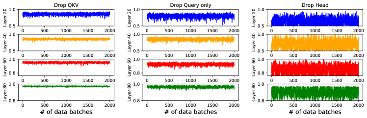
Figure 5: Cosine similarity of weights gradient for different method on applying SBP on ViT-Tiny MHSA layers with a keep-ratio of 0.5. Left: Drop QKV, middle: Drop Query only, right: Drop Head.

5 Generalizability of SBP

We evaluate the generalizability of our proposed SBP on two computer vision benchmarks: image classification on ImageNet [18] and object detection on COCO [10]. In order to do a fair comparison of the same network, we keep the training hyper-parameters of optimizer, augmentation, regularization, batch size and learning rate the same for a given model, and only adopt different stochastic depth augmentation [9] for different model sizes. The Mixed Precision Training [17] method is enabled for faster training. All experiments are conducted on machines with 8$\times$ Tesla 16GB V100. Each accuracy is reported with an average result of three runs with different random seeds. For more details of experimental settings, please refer to the supplementary material.

5.1 Classification on ImageNet

We report the memory and accuracy trade-off in Tab. 1 for two state-of-the-art networks: transformer-based ViT [6] and convolutional-based ConvNeXt [14]. We train 300 epochs for both these two networks by following the training recipe of ConvNeXt [14].

For ViT models, we apply SBP on the last 8 transformer blocks including MHSA and MLP layers with the keep-ratio of 0.5, reducing GPU memory usage by approximately 30%. Note that the memory saving ratio of the network is not proportional the the drop-ratio ($1-$ keep-ratio) because we only apply SBP on $\frac{2}{3}$ of all the layers. With keep ratio of 0.5, the SBP technique can still effectively learn with an accuracy drop of only 0.59% and 0.62% for ViT-Tiny and ViT-Base, respectively.

For ConvNeXt models, it builds the basic block with a depth-wise convolutional (DW-Conv) layer with kernel size $7\times 7$ followed by two point-wise convolutional (PW-Conv) layers and the DW-Conv layer only consumes a small portion of GPU memory (less than 10%). It has multi-scale stages where early stages have higher redundancy and occupy most of the GPU memory. Therefore, we apply SBP on the PW-Conv and down-sampling layers in the first three stages, and do not apply it on the last stage. With a keep ratio of 0.5, ConvNeXt-Tiny and ConvNeXt-Base can efficiently learn the model with a GPU memory saving of above 40% and an accuracy drop within 0.53%.

Table 1: Accuracy and memory results of applying SBP for ViT and ConvNeXt on ImageNet.

Network	Keep-ratio	Batch size	Memory (MB / GPU)	Top-1 accuracy (%)
ViT-Tiny	no SBP	256	8248	73.68
ViT-Tiny	0.5	256	5587 ($0.68\times$)	73.09 (-0.59)
ViT-Base	no SBP	64	10083	81.22
ViT-Base	0.5	64	7436 ($0.74\times$)	80.62 (-0.60)
ConvNeXt-Tiny	no SBP	128	12134	82.1
ConvNeXt-Tiny	0.5	128	7059 (0.58$\times$)	81.61 (-0.49)
ConvNeXt-Base	no SBP	64	14130	83.8
ConvNeXt-Base	0.5	64	8758 (0.62$\times$)	83.27 (-0.53)

5.2 Object Detection and Segmentation on COCO

We fine-tune Mask R-CNN [8] and Cascade Mask R-CNN [1] on the COCO dataset [10] with ConvNeXt-Tiny and ConvNeXt-Base backbones pretrained on ImageNet-1K, respectively. Following the same hyper-parameter settings of [14], we apply SBP on the ConvNeXt backbones to save training memory. Results in Tab. 2 show that SBP with keep-ratio of 0.5 can still learn the detection task reasonably well with 0.2% and 0.7% loss on the box and mask average precision (AP) for ConvNeXt-Base and ConvNeXt-Tiny backbones, respectively. However, it only consumes about 0.7$\times$ of the GPU memory.

Note that training detection models on high resolution images (up to 800$\times$1333) is memory intensive even for a very small batch size, e.g., with backbone of ConvNeXt-Base and batch size of 2, the training requires 17.4GB of GPU memory which may lead to out of memory error for common devices such as Tesla 16GB V100. While with the help of SBP, the model can still be effectively trained on GPUs with 12.5GB memory, which is much more feasible for many research groups. Here we apply SBP only in the backbone, we believe it has a potential to apply SBP on more other layers in the detection model to achieve more promising results in terms of memory efficiency.

Table 2: COCO object detection and segmentation results using Mask-RCNN with backbone ConvNeXt-T and Cascade Mask-RCNN with backbone ConvNeXt-B.

Backbone	Keep- ratio	Batch size	Memory (GB / GPU)	$\text{AP}^{\text{box}}$	$\text{AP}^{\text{box}}_{50}$	$\text{AP}^{\text{box}}_{75}$	$\text{AP}^{\text{mask}}$	$\text{AP}^{\text{mask}}_{\text{50}}$	$\text{AP}^{\text{mask}}_{75}$
ConvNeXt-T	no SBP	2	8.6	46.2	67.9	50.8	41.7	65.0	44.9
ConvNeXt-T	0.5	2	5.9 (0.69$\times$)	45.5	67.4	50.1	41.1	64.4	44.1
ConvNeXt-B	no SBP	2	17.4	52.7	71.3	57.2	45.6	68.9	49.5
ConvNeXt-B	0.5	2	12.5 (0.72$\times$)	52.5	71.3	57.2	45.4	68.7	49.2

6 Discussion

In this work, we present a comprehensive study of the Stochastic Backpropagation (SBP) mechanism with a generalized implementation. We analyze the effect of different design strategies to optimize the trade-off between accuracy and memory. We show that our approach can reduce up to 40% of the GPU memory when training image recognition models under various deep learning backbones.

Limitations: In general, SBP is a memory efficient training method, but it still causes slight loss of accuracy. In our current results, SBP produces only a small amount of training speedup($\sim 1.1\times$). How to further speed up the training process is part of our future work.

Societal impact: Our work studies the stochastic backpropagation mechanism, which can be used for training general deep learning models. Misuse can potentially cause societal harm. However, we believe our work is a general approach and is consist with the common practice in machine learning.

7 Acknowledgments and Disclosure of Funding

We thank the anonymous reviewers for their helpful suggestions. This work was funded by Amazon.

Checklist

1. For all authors…

   1. Do the main claims made in the abstract and introduction accurately reflect the paper’s contributions and scope? [Yes]

   2. Did you describe the limitations of your work? [Yes] See Section 6.

   3. Did you discuss any potential negative societal impacts of your work? [Yes] See Section 6.

   4. Have you read the ethics review guidelines and ensured that your paper conforms to them? [Yes]

2. If you are including theoretical results…

   1. Did you state the full set of assumptions of all theoretical results? [N/A]

   2. Did you include complete proofs of all theoretical results? [N/A]

3. If you ran experiments…

   1. Did you include the code, data, and instructions needed to reproduce the main experimental results (either in the supplemental material or as a URL)? [Yes] See Section 5’s first paragraph and Section 8.3 in the supplementary material.

   2. Did you specify all the training details (e.g., data splits, hyperparameters, how they were chosen)? [Yes] See Section 5’s first paragraph and Section 5.1’s first paragraph.

   3. Did you report error bars (e.g., with respect to the random seed after running experiments multiple times)? [Yes] Each accuracy report is an average result of running experiments three times with different random seeds.

   4. Did you include the total amount of compute and the type of resources used (e.g., type of GPUs, internal cluster, or cloud provider)? [Yes] See Section 5’s first paragraph and Section 8.3 in the supplementary material.

4. If you are using existing assets (e.g., code, data, models) or curating/releasing new assets…

   1. If your work uses existing assets, did you cite the creators? [Yes] We cited the all datasets we used, such as ImageNet [18] ad COCO [10].

   2. Did you mention the license of the assets? [No] ImageNet is under BSD 3-Clause License and COCO is under Creative Commons Attribution 4.0 License.

   3. Did you include any new assets either in the supplemental material or as a URL? [No]

   4. Did you discuss whether and how consent was obtained from people whose data you’re using/curating? [No]

   5. Did you discuss whether the data you are using/curating contains personally identifiable information or offensive content? [No] We do not have sufficient resource to exhaustively screen offensive content from the datasets we used. We expect, because the datasets only contain images of people with daily activities and common objects, they are unlikely to contain offensive content. They are both very widely used.

5. If you used crowdsourcing or conducted research with human subjects…

   1. Did you include the full text of instructions given to participants and screenshots, if applicable? [N/A]

   2. Did you describe any potential participant risks, with links to Institutional Review Board (IRB) approvals, if applicable? [N/A]

   3. Did you include the estimated hourly wage paid to participants and the total amount spent on participant compensation? [N/A]

 

An In-depth Study of Stochastic Backpropagation

 

8 Supplementary material

In this supplementary material, we expand our discussion on Stochastic Backpropagation (SBP) with additional analysis and experiments. In particular, we discuss the following:

• Section 8.1 derives the gradient calculation for attention layers.

• Section 8.2 discusses the chain rule effect on the transformer blocks.

• Section 8.3 reports the details of the experiment settings.

• Section 8.4 investigates the insights on the gradient keep-ratios and gradient keep masks on a very deep network ConvNeXt-Base.

• Section 8.5 discusses the vanishing gradient problem.

• Section 8.6 compares the model similarity between with and without applying SBP.

8.1 Gradient Calculation of Attention Layers

In section 3.2, we provide the gradient calculation of linear layers (or PW-Conv) and general convolutional layers for the backward phase of SBP. Here we derive the equations to the attention layers, as they are the important layers in the transformer-based architectures [6, 11].

In the original multi-head self-attention (MHSA) module of vision transformers [6], given a layer $i$, it first linearly transforms the input tensor $X_{i}\in\mathbb{R}^{B\times N_{i}\times C_{i}}$ (flatten from feature map $X_{i}\in\mathbb{R}^{B\times T_{i}\times H_{i}\times W_{i}\times C_{i}}$) to query tensor $Q_{i}\in\mathbb{R}^{(B\times N_{i})\times(h\times d_{Q_{i}})}$, key tensor $K_{i}\in\mathbb{R}^{(B\times N_{i})\times(h\times d_{K_{i}})}$, value tensor $V_{i}\in\mathbb{R}^{(B\times N_{i})\times(h\times d_{V_{i}})}$ by linear layers with learnable weights $W_{Q_{i}}\in\mathbb{R}^{C_{i}\times(h\times d_{Q_{i}})}$, $W_{K_{i}}\in\mathbb{R}^{C_{i}\times(h\times d_{K_{i}})}$, $W_{V_{i}}\in\mathbb{R}^{C_{i}\times(h\times d_{V_{i}})}$. The query $Q_{i}$, key $K_{i}$, value $V_{i}$ and their corresponding weights $W_{Q_{i}}$, $W_{K_{i}}$, $W_{V_{i}}$ are reshaped as a matrix format. The notation $N_{i}=T_{i}\times H_{i}\times W_{i}$ is the number of tokens, $h$ is the number of heads, and $d_{Q_{i}}$, $d_{K_{i}}$ and $d_{V_{i}}$ are the dimensions of query, key and value, respectively. The forward pass of these three linear mapping is

$$Q_{i}=X_{i}W_{Q_{i}},\quad K_{i}=X_{i}W_{K_{i}},\quad V_{i}=X_{i}W_{V_{i}}.$$ (14)

It then calculates a scaled dot-product attention,

$$\begin{array}[]{ll}&M_{i}=\frac{Q_{i}K_{i}^{T}}{\sqrt{d_{K_{i}}}},\quad S_{i}=\mbox{softmax}(M_{i}),\vspace{2mm}\\ &X_{i+1}=A_{i}=\mbox{Attention}(Q_{i},K_{i},V_{i})=\mbox{softmax}\left(\frac{Q_{i}K_{i}^{T}}{\sqrt{d_{K_{i}}}}\right)V_{i}=S_{i}V_{i}\end{array}$$ (15)

During the traditional backward pass with full backpropagation, the gradients of query, key, value are calculated by

$$dQ_{i}=dM_{i}\frac{K_{i}}{\sqrt{d_{K_{i}}}},\quad dK_{i}=\frac{Q_{i}^{T}}{\sqrt{d_{K_{i}}}}dM_{i},\quad dV_{i}=S_{i}^{T}dA_{i}.$$ (16)

The gradients of weights $W_{Q_{i}}$, $W_{K_{i}}$, $W_{V_{i}}$ are as follows

$$dW_{Q_{i}}=X_{i}^{T}dQ_{i},\quad dW_{K_{i}}=X_{i}^{T}dK_{i},\quad dW_{V_{i}}=X_{i}^{T}dV_{i},$$ (17)

and the gradient of input $X_{i}$ is

$$dX_{i}=dQ_{i}W_{Q_{i}}+dK_{i}W_{K_{i}}+dV_{i}W_{V_{i}}.$$ (18)

To apply SBP on the MHSA layers, we apply gradients dropout on the attention map $M_{i}$ (has dimension $hN_{i}^{2}$) instead of the feature map $X_{i+1}$ (has dimension $hd_{V_{i}}N_{i}$) because the attention map $M_{i}$ dominants the memory usage as $N_{i}>d_{V_{i}}$. We refer to section 4 and Eq. (13) for more details of the memory usage.

We also have different choices of dropping gradients and here we give an example of dropping on query only, other methods such as dropping on heads or dropping on all QKV can be easily derived in a similar way. Similar to the analysis of linear layer case in section 3.2.1, we split the query tensor into two subsets $Q_{i}^{keep}$ and $Q_{i}^{drop}$ along the spatial dimension, and the forward spatial nodes in query tensor $Q_{i}$ and the attention weights maps $M_{i}$ can be calculated independently as:

$$\begin{array}[]{ll}&Q_{i}^{keep}=X_{i}^{keep}W_{Q_{i}},\quad Q_{i}^{drop}=X_{i}^{drop}W_{Q_{i}},\vspace{2mm}\\ &M_{i}^{keep}=\frac{Q_{i}^{keep}K_{i}^{T}}{\sqrt{d_{K_{i}}}},\quad M_{i}^{drop}=\frac{Q_{i}^{drop}K_{i}^{T}}{\sqrt{d_{K_{i}}}}.\end{array}$$ (19)

Regarding to the backward, SBP drops gradients with superscripts ^drop on $Q_{i}$ and $M_{i}$. It sets $dM_{i}^{drop}=\textbf{0}$ and has

$$\begin{array}[]{ll}&dQ_{i}=[dQ_{i}^{keep},dQ_{i}^{drop}],\vspace{2mm}\\ &dQ_{i}^{keep}=\frac{1}{\sqrt{d_{K_{i}}}}dM_{i}^{keep}K_{i}^{T},\vspace{2mm}\\ &dQ_{i}^{drop}=\frac{1}{\sqrt{d_{K_{i}}}}dM_{i}^{drop}K_{i}^{T}=\textbf{0},\end{array}$$ (20)

and

$$\begin{array}[]{ll}dK_{i}&=\frac{1}{\sqrt{d_{K_{i}}}}Q_{i}^{T}dM_{i}=\frac{1}{\sqrt{d_{K_{i}}}}[Q_{i}^{keep},Q_{i}^{drop}]^{T}[dM_{i}^{keep},dM_{i}^{drop}],\vspace{2mm}\\ &=\frac{1}{\sqrt{d_{K_{i}}}}({Q_{i}^{keep}}^{T}dM_{i}^{keep}+{Q_{i}^{drop}}^{T}dM_{i}^{drop})=\frac{1}{\sqrt{d_{K_{i}}}}{Q_{i}^{keep}}^{T}dM_{i}^{keep}.\end{array}$$ (21)

That is, the query $Q_{i}$ has exact gradients on the kept locations and zero gradients on the dropped locations, and the gradient of key $dK_{i}$ has neither exact nor zero gradients but estimated by $\frac{1}{\sqrt{d_{K_{i}}}}{Q_{i}^{keep}}^{T}dM_{i}^{keep}$.

Since there is no gradient dropout on the value tensor $V_{i}$, from Eq. (17), it’s gradient $dV_{i}$ will not be affected by SBP and will be the same to the gradient (we call it the exact gradient) of the model without applying SBP.

However, the gradients of query and key weights will be updated and not be the same to the original case without applying SBP. More specifically, we have the gradients of query weights

$$\begin{array}[]{ll}dW_{Q_{i}}&=X_{i}^{T}dQ_{i}=[X_{i}^{keep},X_{i}^{drop}]^{T}[dQ_{i}^{keep},dQ_{i}^{drop}]\vspace{2mm}\\ &={X_{i}^{keep}}^{T}dQ_{i}^{keep}+{X_{i}^{drop}}^{T}dQ_{i}^{drop}={X_{i}^{keep}}^{T}dQ_{i}^{keep}\end{array}$$ (22)

and the gradients of key weights

$$\begin{array}[]{ll}dW_{K_{i}}&=X_{i}^{T}dK_{i}=\frac{1}{\sqrt{d_{K_{i}}}}X_{i}^{T}{Q_{i}^{keep}}^{T}dM_{i}^{keep}.\end{array}$$ (23)

They are all calculated as an approximated version of their original gradients by only using the feature maps at the kept indices. From Eq. (20) and  (21), we can also update the gradients of input $X_{i}$ in Eq. (18) and it will be an approximated version of its original case as well.

8.2 Chain Rule Effect of Transformer Blocks

In general, transformer block consists of two sub-blocks: Multi-Head Self-Attention (MHSA) and Multi-layer perception (MLP). The MLP sub-block is equivalent to two PW-Conv or linear layers. In section 3.3.1, we discuss the chain rule effect on two consecutive PW-Conv layers $f_{i}$ and $f_{i-1}$, here we extend the chain rule effect to the previous MHSA layers $f_{i-2}$. From section 3.3.1 and 4 (Fig. 2 right), using uniform keep-ratios and having the same gradients dropping indices set on consecutive layers can preserve more gradient information and gain higher accuracy, thus in this section we only consider the same keeping and dropping indices on the entire transformer block. That is, $\mathbb{Z}_{i+1}^{keep}=\mathbb{Z}_{i}^{keep}=\mathbb{Z}_{i-1}^{keep}$ and $\mathbb{Z}_{i+1}^{drop}=\mathbb{Z}_{i}^{drop}=\mathbb{Z}_{i-1}^{drop}$.

From 3.3.1, $dX_{i-1}$ has non-zero gradients (which are exact to the original case without SBP) at kept indices and zero gradients at dropped indices. By chain rule, the backward gradients pass to the MHSA layer output $A_{i-2}$ and we have $A_{i-2}^{keep}$ to be exact gradients and $A_{i-2}^{drop}=\textbf{0}$. From the Eq. (15), (16), and (17), the gradients of value tensor $dV_{i-2}$ and value weights $dW_{V_{i-2}}$ will be all affected and no longer be the exact. Therefore, the gradients of all QKV weights and activations will be updated and calculated as an estimation to the original gradients of mini-batch SGD without applying SBP.

8.3 Experimental Settings

In this section, we report the experimental details of training settings. For ImageNet training of both ViT and ConvNeXt, we follow the same hyper-parameter settings of Table. 5 in [14] except that we use different stochastic depth rates for different models. Specifically, we set stochastic depth rates 0.0, 0.5, 0.1, 0.5 (and 0.0, 0.3, 0.1, 0.3) for ViT-Tiny, ViT-Base, ConvNeXt-Tiny, ConvNeXt-Base without applying SBP (and with applying SBP with a keep-ratio of 0.5), respectively. For ViT-Tiny and ViT-Base, we apply SBP on the last 8 transformer blocks. For ConvNeXt-Tiny and ConvNeXt-Base, we apply SBP on all blocks of the first two stages. On the third stages, we apply SBP on the first 6, 21 blocks for ConvNeXt-Tiny, ConvNeXt-Base, respectively. We use one machine (each machine has 8$\times$ Tesla 16GB V100) to train ViT-Tiny and ConvNeXt-Tiny and 4 machines to train ViT-Base and ConvNeXt-Base.

For COCO experiments, we follow the same training settings used in Section A.3. of [14]. We only apply SBP on the ConvNeXt backbones. We use the backbone weights pre-trained from ImageNet as network initializations. We use one machine to train the detection task.

8.4 Gradient Keep-ratios and Keep Masks on ConvNeXt-Base

We further investigate the insights on the gradient keep-ratios and gradient keep masks on a very deep network, ConvNeXt-Base, which has more than 100 layers. We plot the cosine similarity of weights gradient between with and without applying SBP on layer 20, 50, 80, 110 of ConvNeXt-Base, which are PW-Conv1, DW-Conv, PW-Conv2, DW-Conv layers, respectively.

From Fig. 6, we also observe that the uniform keep-ratios method has an overall stronger correlation compared to non-uniform keep-ratios methods. More specifically, compared to uniform keep-ratios method, decreasing keep-ratios method has a weaker correlation on deeper layers as the keep-ratios are smaller in the deeper layers. Although the increasing keep-ratios method enjoys a stronger correlation on deeper layers, it has a smaller gradient keep-ratio as well as a weaker correlation in early layers. This observation is consistent between the ViT and ConvNeXt networks.

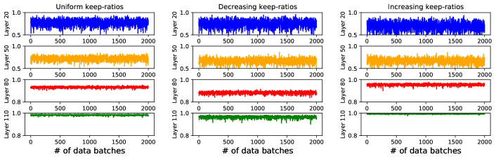
Figure 6: Cosine similarity of weights gradient between with and without applying SBP on ConvNeXt-Base with uniform, decreasing, and increasing keep-ratios.

Next, we compare the grid-wise sampling mask and random sampling mask. In the training process, we randomly sample the gradient keep mask in every iteration so that every spatial location will be statistically visited with equal importance. Once the mask is sampled in each iteration, we apply uniform keep-ratios for every SBP layer with the same gradient keep mask. Fig. 7 gives a particular example of the sampled masks for 5 iterations with a keep-ratio of 0.5. In the first two iterations (upper left of Fig. 7), the grid-wise sampling can visit all spatial locations, which is not observed in the random sampling. In Fig. 8, it is also observed that the grid-wise sampling achieves a stronger correlation compared to the random sampling. In general, the correlation behaviors of gradient keep-ratios methods and gradient sampling methods are consistent to both ViT and ConvNeXt networks.

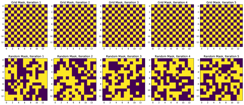
Figure 7: A particular example of sampled gradient keep masks for 5 iterations. Keep-ratio is 0.5. Upper: grid-wise sampling method. Lower: random sampling method.

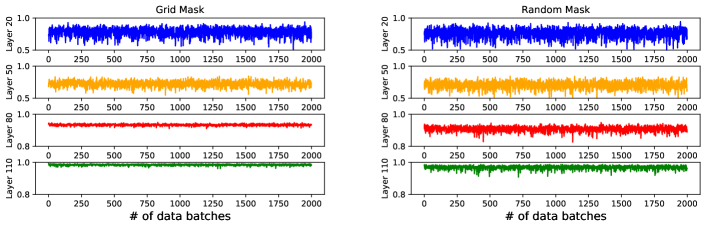
Figure 8: Cosine similarity of weights gradient between with and without applying SBP-0.5 on ConvNeXt-Base with grid-wise sampling and random sampling method.

8.5 Vanishing Gradients?

We plot the L2 norm of weight gradients of some or all layers of the model during training process for ViT-Tiny (Fig. 9) and ConvNeXt-Base (Fig. 10). Although SBP discards some parts of gradient information, especially on activations, we did not observe the vanishing gradient problem on weights. However, from (10) and (11), in an extreme case that two consecutive SBP layers have non-overlapped keep indices, i.e., $\mathbb{Z}_{i+1}^{keep}\cap\mathbb{Z}_{i}^{keep}=\emptyset$, the gradient information on all indices will be dropped, and therefore, the vanishing gradient occurs. We point out that this is never the case in practice and it can be simply avoided by using the same gradient keep mask across all SBP layers.

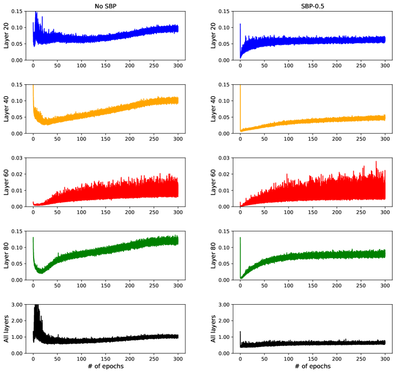
Figure 9: L2 norms of weights gradient on some or all layers of ViT-Tiny. Left: baseline without applying SBP. Right: with applying SBP-0.5.

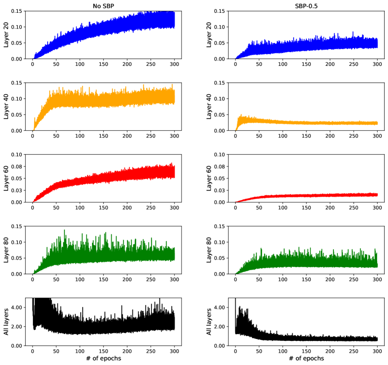
Figure 10: L2 norms of weights gradient on some or all layers of ConvNeXt-Base. Left: baseline without applying SBP. Right: with applying SBP-0.5.

8.6 Model Similarity

We plot the cosine similarity of model weights in Fig. 11 to show the change curve during the entire training process. The training hyper-parameters and model initialization weights are the same for model trained with and without applying SBP. We observe that the cosine similarity of model weights gradually decay from 1.00 to 0.14 for ViT-Tiny and 0.06 for ConvNeXt-Base, which indicates that the final model weights may not be similar after the dynamic training process. One explanation is that at the early stage of training, model weights with SBP only show a small difference compared to those without SBP. However, as the the training goes further and further, this small difference will be propagated and become larger and larger.

We also evaluate the sample-level top-1 prediction consistency rate between models trained with and without applying SBP. For ViT-Tiny and ConvNeXt-Base cases, the consistency rates on ImageNet validation dataset are 80.73% and 91.12%, respectively. The consistency rates are much higher than their corresponding top-1 accuracies, which demonstrates that models trained with or without applying SBP can can take different learning paths and end up with different local minima, but with similar prediction performance.

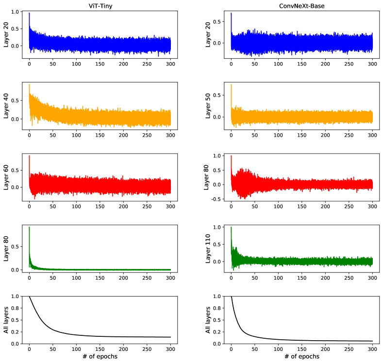
Figure 11: Cosine similarity of model weights on some or all layers between models with and without applying SBP-0.5.

References

- Cai and Vasconcelos [2018] Zhaowei Cai and Nuno Vasconcelos. Cascade r-cnn: Delving into high quality object detection. In CVPR, 2018.
- Chen et al. [2016] Tianqi Chen, Bing Xu, Chiyuan Zhang, and Carlos Guestrin. Training deep nets with sublinear memory cost. arXiv:1604.06174, 2016.
- Cheng et al. [2022] Feng Cheng, Mingze Xu, Yuanjun Xiong, Hao Chen, Xinyu Li, Wei Li, and Wei Xia. Stochastic backpropagation: A memory efficient strategy for training video models. CVPR, 2022.
- Dai et al. [2021] Zihang Dai, Hanxiao Liu, Quoc V Le, and Mingxing Tan. Coatnet: Marrying convolution and attention for all data sizes. NeurIPS, 2021.
- Dettmers and Zettlemoyer [2019] Tim Dettmers and Luke Zettlemoyer. Sparse networks from scratch: Faster training without losing performance. arXiv:1907.04840, 2019.
- Dosovitskiy et al. [2020] Alexey Dosovitskiy, Lucas Beyer, Alexander Kolesnikov, Dirk Weissenborn, Xiaohua Zhai, Thomas Unterthiner, Mostafa Dehghani, Matthias Minderer, Georg Heigold, Sylvain Gelly, et al. An image is worth 16x16 words: Transformers for image recognition at scale. arXiv:2010.11929, 2020.
- He et al. [2016] Kaiming He, Xiangyu Zhang, Shaoqing Ren, and Jian Sun. Deep residual learning for image recognition. In CVPR, 2016.
- He et al. [2017] Kaiming He, Georgia Gkioxari, Piotr Dollár, and Ross Girshick. Mask r-cnn. In ICCV, 2017.
- Huang et al. [2017] Gao Huang, Zhuang Liu, Laurens van der Maaten, and Kilian Q Weinberger. Densely connected convolutional networks. In CVPR, 2017.
- Lin et al. [2014] Tsung-Yi Lin, Michael Maire, Serge Belongie, James Hays, Pietro Perona, Deva Ramanan, Piotr Dollár, and C Lawrence Zitnick. Microsoft coco: Common objects in context. In ECCV, 2014.
- Liu et al. [2021a] Ze Liu, Yutong Lin, Yue Cao, Han Hu, Yixuan Wei, Zheng Zhang, Stephen Lin, and Baining Guo. Swin transformer: Hierarchical vision transformer using shifted windows. In ICCV, 2021a.
- Liu et al. [2021b] Ze Liu, Yutong Lin, Yue Cao, Han Hu, Yixuan Wei, Zheng Zhang, Stephen Lin, and Baining Guo. Official Implementation of Swin transformer. https://github.com/microsoft/Swin-Transformer, 2021b. [Online; accessed 12-Sep-2022].
- Liu et al. [2021c] Ze Liu, Jia Ning, Yue Cao, Yixuan Wei, Zheng Zhang, Stephen Lin, and Han Hu. Video swin transformer. arXiv:2106.13230, 2021c.
- Liu et al. [2022] Zhuang Liu, Hanzi Mao, Chao-Yuan Wu, Christoph Feichtenhofer, Trevor Darrell, and Saining Xie. A convnet for the 2020s. CVPR, 2022.
- Malinowski et al. [2020] Mateusz Malinowski, Grzegorz Swirszcz, Joao Carreira, and Viorica Patraucean. Sideways: Depth-parallel training of video models. In CVPR, 2020.
- Malinowski et al. [2021] Mateusz Malinowski, Dimitrios Vytiniotis, Grzegorz Swirszcz, Viorica Patraucean, and Joao Carreira. Gradient forward-propagation for large-scale temporal video modelling. In CVPR, 2021.
- Micikevicius et al. [2017] Paulius Micikevicius, Sharan Narang, Jonah Alben, Gregory Diamos, Erich Elsen, David Garcia, Boris Ginsburg, Michael Houston, Oleksii Kuchaiev, Ganesh Venkatesh, et al. Mixed precision training. arXiv:1710.03740, 2017.
- Russakovsky et al. [2015] Olga Russakovsky, Jia Deng, Hao Su, Jonathan Krause, Sanjeev Satheesh, Sean Ma, Zhiheng Huang, Andrej Karpathy, Aditya Khosla, Michael Bernstein, et al. Imagenet large scale visual recognition challenge. IJCV, 2015.
- Tan and Le [2019] Mingxing Tan and Quoc Le. Efficientnet: Rethinking model scaling for convolutional neural networks. In ICML, 2019.
- Wu et al. [2020] Chao-Yuan Wu, Ross Girshick, Kaiming He, Christoph Feichtenhofer, and Philipp Krahenbuhl. A multigrid method for efficiently training video models. In CVPR, 2020.
- Xie et al. [2017] Saining Xie, Ross Girshick, Piotr Dollár, Zhuowen Tu, and Kaiming He. Aggregated residual transformations for deep neural networks. In CVPR, 2017.
- Xu et al. [2020] Mengmeng Xu, Chen Zhao, David S Rojas, Ali Thabet, and Bernard Ghanem. G-tad: Sub-graph localization for temporal action detection. In CVPR, 2020.
- Xu et al. [2019] Mingze Xu, Mingfei Gao, Yi-Ting Chen, Larry S Davis, and David J Crandall. Temporal recurrent networks for online action detection. In ICCV, 2019.
- Xu et al. [2021] Mingze Xu, Yuanjun Xiong, Hao Chen, Xinyu Li, Wei Xia, Zhuowen Tu, and Stefano Soatto. Long short-term transformer for online action detection. NeurIPS, 2021.