Factorized Fusion Shrinkage for Dynamic Relational Data

Abstract

Modern data science applications often involve complex relational data with dynamic structures. In systems that experience regime changes, such as changes in alliances between nations after a war or air transportation networks in the wake of the COVID-19 pandemic, abrupt alterations in the relational dynamics of such data are commonly observed. To address this scenario, we propose a Factorized Fusion Shrinkage Model, which consists of a dynamic shrinkage of each decomposed factor towards a group-wise fusion structure, where shrinkage is achieved through the application of global-local shrinkage priors to successive differences in the row vectors of the factorized matrices. The priors employed in the model preserve both the separability of clusters and the long-range properties of latent factor dynamics. Under specific conditions, we prove that the posterior distribution of the model attains the minimax optimal rate up to logarithmic factors. In terms of computation, we introduce a structured mean-field variational inference algorithm that balances optimal posterior inference with computational scalability. This framework leverages both the inter-component dependence and the temporal dependence across time. Our framework is versatile and can accommodate a wide range of models, including latent space models for networks, dynamic matrix factorization, and low-rank tensor models. The efficacy of our methodology is tested through extensive simulations and real-world data analysis.

Keywords: Bayesian low-rank modeling; post-processing; posterior contraction; structured shrinkage; tensor data; variational inference

1 Introduction

Relational data describes the relationship between two or more sets of variables and is typically observed as matrices or multi-way arrays/tensors. One of the objectives of relational data analysis is to explain the variation in the entries of a relational array through unobserved explanatory factors. For example, given matrix-valued data $\boldsymbol{Y}\in\mathbb{R}^{n\times p}$, the static low-rank plus noise model of the form $\boldsymbol{Y}=\boldsymbol{U}\boldsymbol{V}^{\prime}+\boldsymbol{E}$, where $\max\{\mbox{rank}(\boldsymbol{U}),\mbox{rank}(\boldsymbol{V})\}\ll\min\{n,p\}$ and $\boldsymbol{E}$ is an error term, has been extensively studied; see Hoff, (2007); Chatterjee, (2015); Gavish and Donoho, (2014); Donoho et al., (2020) for a flavor and connections with truncated singular value decompositions.

Recent decades have seen a rapidly growing interest in analyzing dynamic, complex data sets in the era of data science. Models for dynamic relational data have found wide applications in numerous practice areas, including dynamic social network analysis (Sarkar and Moore,, 2005; Zhu et al.,, 2016), subspace tracking (Doukopoulos and Moustakides,, 2008), traffic prediction (Tan et al.,, 2016), recommendation system (Zhang et al.,, 2021) among others. Compared to static relational data, additional challenges are posed when the observation matrices possess a dynamic structure. Critically, modeling the evolution of $\boldsymbol{Y}_{t},t=1,...,T$ over time is vital. This is commonly achieved by specifying a parsimonious probability model for $\boldsymbol{Y}_{t}$ involving lower-dimensional latent/hidden variables at each time point $t$, and then specifying an appropriate evolution of these observations or latent variables over time. For example, the classical vector autoregressive (VAR) model (Stock and Watson,, 2016; Lütkepohl,, 2013) has been employed to model the evolution of the observations directly; Sarkar and Moore, (2005) used an AR(1) type of evolution of the latent factors in the context of latent space models for dynamic networks; Hoff, (2011) parameterized time-varying latent factors in terms of static factors with time-varying weights for a three-way tensor model; Hoff, (2015) considered a bi-linear autoregressive model and Friel et al., (2016) modeled the evolution by considering evolving observation-related parameters as well as latent factors in a bipartite network model.

Abrupt changes are important examples of non-stationarity, typically observed in systems that undergo regime changes due to an intervention, such as alliances between nations before/after a war (Gibler,, 2008), voting records before and after an election (Lee et al.,, 2004), or the impact of protein networks after a treatment (Hegde et al.,, 2008). This article presents a novel shrinkage process for dynamic relational data to handle such abrupt changes adaptively.

Given the dynamic likelihood $\boldsymbol{Y}_{t}=\boldsymbol{U}_{t}\boldsymbol{V}_{t}^{\prime}+\boldsymbol{E}_{t}$, $t=1,...,T$, we introduce time-dependence by shrinking the successive differences between the row vectors $\{\boldsymbol{u}_{it}\},\{\boldsymbol{v}_{it}\}$ of $\boldsymbol{U}_{t}$, $\boldsymbol{V}_{t}$ to group-wise sparse vectors. In particular, we propose a factorized fusion shrinkage (FFS) prior, where group-wise global-local shrinkage priors on all the transitions of latent factors are applied to promote group-wise fusion structures. The adopted global-local prior has a sufficient mass around zero, effectively shrinking transitions to zeros while keeping large enough transitions, promoting fusion structures. In addition, all components of the transitions share the same local scales from the prior, leading to interpretable group-wise shrinkage. The proposed model attempts to account for the dynamic change and dependence across $\boldsymbol{Y}_{t}$ by reflecting the piecewise constant changes among the row and column factors, $\boldsymbol{U}_{t}$ and $\boldsymbol{V}_{t}$. The symmetric version of the model is also useful for network models, where one requires that $\boldsymbol{U}_{t}=\boldsymbol{V}_{t}$ for $t=1,...,T$. In addition, we extend the model to tensor data under the CANDECOMP/PARAFAC (CP) type of low-rank structure.

The proposed FFS priors differ substantially from those in literature analyzing dynamic relational data, like normal transition priors with a common variance and Gaussian process priors (Sarkar and Moore,, 2005; Sun et al.,, 2014; Sewell and Chen,, 2015; Durante and Dunson,, 2014; Sewell and Chen,, 2017; Zhang et al.,, 2018). While the above commonly used dynamic priors tend to introduce the smoothness effect among dynamic transitions, FFS priors are designed to introduce the stopping and separation effects so that the transitions are either closed to zeros or large. In particular, the stopping effect of FFS priors can significantly enhance the interpretation of the dynamics of latent vectors. As an illustration, we present one simulation example (see subsection 8.2.2 in the supplement for details) to illustrate the effect of FFS prior by comparing it with the latent space model with a commonly used normal-inverse-gamma prior on the transitions (IGLSM, e.g., equation (2) in Sewell and Chen, (2015)) in the dynamic network settings. Figure 1 shows an example in which only subjects $1$ and $2$ change over time. With IGLSM, all subjects change in a small magnitude in the estimated latent space, so it is difficult to identify subjects $1$ and $2$ among all the other subjects, whereas with FFS, only the subjects $1$ and $2$ change significantly at the correct time point.

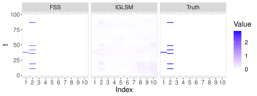
Figure 1: Heatmaps of matrices whose components are $\ell_{2}$ norm of transitions $\{\|D\boldsymbol{u}_{it}\|\}_{i=1,...,10;\,t=2,...,T}$ with $D\boldsymbol{u}_{it}=\boldsymbol{u}_{i(t+1)}-\boldsymbol{u}_{it}$ after estimating latent vectors by FFS priors, IGLSM and the truth correspondingly. Index: subject index; $t:$ time of the transitions. For IGLSM and FFS prior, Procrustes rotation (6) is performed where the latent vectors of time $t=2,..,T$ are projected to the locations that are most close to its previous locations. FFS priors can better identify the time and subjects of transitions than IGLSM when the true transitions are sparse.

Furthermore, the separation effect of FFS priors contributes to the detection of clusters among subjects after estimating the latent factors. The detected cluster results provide information on which subjects have similar effects in generating the relational data. When performing clustering algorithms such as $K$-means, the cluster separation $\delta_{t}=\min_{i\neq j}\|\boldsymbol{u}_{it}-\boldsymbol{u}_{jt}\|_{2}$ for any $\boldsymbol{u}_{it},\boldsymbol{u}_{jt}$ not in the same cluster plays a crucial role in determining the difficulty level of the problem (e.g., eigengap for spectral clustering, see Ng et al., (2001)). Generally, the larger $\delta_{t}$ is, the easier it is to detect clusters at time $t$. The separation effect of FFS priors is justified by encouraging more separate clusters: Suppose at time $t$ we have $\boldsymbol{u}_{it}=\boldsymbol{u}_{jt}$ for subjects $i,j$, and at time $t+1$, subject $i$ moves to another cluster while subject $j$ stays in the same cluster. Then the cluster separation at time $t+1$ satisfies $\delta_{t+1}\leq\|\boldsymbol{u}_{j(t+1)}-\boldsymbol{u}_{i(t+1)}\|_{2}=\|\boldsymbol{u}_{j(t+1)}-\boldsymbol{u}_{jt}\|_{2}=\|D\boldsymbol{u}_{jt}\|_{2}$, which highlights the importance of shrinking towards larger transitions. In contrast, priors that introduce smoothness to the transitions tend to impede the separation of the clusters. Overall, the model explicitly links the transitions of latent factors with the changing of cluster memberships for each subject: a zero transition implies no change in cluster membership, while a change in cluster membership implies a large transition.

Dynamic shrinkage priors have been studied in a wide range of literature (Frühwirth-Schnatter and Wagner,, 2010; Chan et al.,, 2012; Nakajima and West,, 2013; Kalli and Griffin,, 2014; Kowal et al.,, 2019). In particular, for dynamic linear models, Kowal et al., (2019) proposed a novel dynamic prior for the transitions with temporal adaptive local scales for their adopted global-local shrinkage prior. In this article, we consider matrix/tensor valued responses with complex dependence structures using a structural dynamic shrinkage model for the transition of the latent factors and illustrate its applicability across a wide range of problems. Additionally, we provide an in-depth theoretical analysis of the proposed prior. We first derive an informative-theoretic lower bound for the model under an appropriate parameter space, incorporating both the initial estimation errors of the matrix/tensor and the selection errors due to the sparsity of the transitions. In addition, we develop an $\ell_{1}$ prior concentration inequality for global-local priors across time when the error rate is also affected by an additional variable other than time due to the multivariate nature of the subjects. Using the proposed prior concentration and a fractional posterior device, we demonstrate that the posterior under the proposed prior can achieve minimax rates up to logarithmic factors. To our knowledge, both the lower bound and posterior concentration are the first results reported in the related literature for dynamic relational data. In addition, it has been established that a frequentist approach cannot achieve this fusion type of minimax optimal rate when $\ell_{1}$-regularization is used (Fan and Guan,, 2018). Therefore, such near-optimal convergence rates improve upon related models via $\ell_{1}$ penalized approaches. Finally, using dynamic network models as an example, we offer theoretical support for the proposed post-processing technique. While posterior post-processing has been increasingly popular in the Bayesian literature, theoretical validations are comparatively rare; see Lee and Lee, (2021) for a recent example in a different context. In particular, community detection and dynamic comparisons are considered under the latent space model, where the truth transitions are assumed to be sparse. Theoretically, we show how the sparsity of the truth transitions and the length of the time range for comparison affect the consistency of the comparison after performing Procrustes rotations. However, it should be noted that the proposed Procrustes rotation approach cannot be immediately applied to a tensor type of model.

From a computational aspect, we present posterior approximations based on variational inference for scalability and computational efficiency while noting that exact MCMC approaches can also be readily developed. We consider a structured mean-field (SMF) variational inference framework, where the group-wise fusion structure, which includes the temporal dependence and the group-wise effect among components, is taken into account. A corresponding coordinate ascent variational inference (Bishop and Nasrabadi, (2006), CAVI) algorithm is developed to incorporate the temporal dependence into the variational inference where simple closed-form updatings can be achieved. The proposed algorithm is more efficient than gradient descent or other first-order algorithm types with little increase in the complexity per iteration since the computation can utilize the banded (or block tri-diagonal) structure of the second-order moments, which incurs a $O(Td^{3})$ cost for matrix inversion compared to a naive approach with $O(T^{3}d^{3})$ cost. Finally, we extend our SMF variational inference framework to tensor data by utilizing a CP type of low-rank factorization.

2 Methodology

2.1 Factorized Fusion Shrinkage

We first lay down the factorized fusion shrinkage (FFS) approach in its most general form for dynamic multi-way arrays before discussing the special case of dynamic matrix-valued data. Specifically, let $\mathcal{Y}=\{\mathcal{Y}_{t}\}_{t=1}^{T}$ be the observed data, where $\mathcal{Y}_{t}\in\mathbb{R}^{n_{1}\times...\times n_{M}}$ is an $M$-way tensor corresponding to the $t$th time point. Examples of such dynamic tensor-valued relational data abound (Boccaletti et al.,, 2014). For example, in the context of daily air transportation networks arising from different airlines providing flights between cities, where the entries of the tensors represent whether the airlines provide flights between two cities on a given date, $\mathcal{Y}_{t}$ is a three-way array with arms representing the city of origin, city of destination, and airlines carrier respectively, and the time-index $t$ runs over days.

For such data, we consider the following dynamic low-rank tensor model:

$$\mathcal{Y}_{t}\sim p(\mathcal{M}_{t};\beta),\quad\mathcal{M}_{t}=\sum_{l=1}^{d}\boldsymbol{u}^{(1)}_{t,l}\otimes...\otimes\boldsymbol{u}^{(M)}_{t,l},\quad t\in[T]:\,=\{1,\ldots,T\},$$ (1)

where $\otimes$ is the vector outer product; $\boldsymbol{u}_{t,l}^{(m)}\in\mathbb{R}^{n_{m}}$ for each $t\in[T]$ and $l\in[d]$; $\mathbb{E}_{p}(\mathcal{Y}_{t}\mid\mathcal{M}_{t})=g(\mathcal{M}_{t})$ for some link function $g$ which operates elementwise on a tensor; and $\beta$ represents additional parameters (e.g., variance, subject-specific effects, etc.) specifying the distribution $p$. For example, an additive tensor Gaussian model assumes the form $\mathcal{Y}_{t}=\mathcal{M}_{t}+\sigma\mathcal{Z}_{t}$, with the entries of $\mathcal{Z}_{t}$ being i.i.d. $N(0,1)$. The decomposition of $\mathcal{M}_{t}$ in equation (1) is based on the CP decomposition (Kolda and Bader,, 2009), which expresses a tensor as a sum of $d$ rank-one tensors, where a rank-one tensor is an outer product of vectors. When $d$ is small compared to $n_{prod}:\,=n_{1}\times\ldots\times n_{m}$, the CP decomposition is highly parsimonious as it reduces the number of bits of information in $\mathcal{M}_{t}$ from $n_{prod}$ to $d\sum_{m=1}^{M}n_{m}$. Alternatively, dynamic tensor models utilizing Tucker decompositions are also widely explored in literature. A good example can be found in Chen et al., (2022).

Even though the CP decomposition vastly reduces the effective number of parameters for static tensor models, additional structural assumptions are necessitated in the dynamic setting to reduce model complexity. We achieve this by proposing a parsimonious yet flexible evolution of latent factor vectors as described below. To that end, we first introduce some notation. For each $m\in[M]$ representing an arm of the tensor, define an $n_{m}\times d$ matrix $\boldsymbol{U}_{t}^{(m)}=[\boldsymbol{u}^{(m)}_{t,1},...,\boldsymbol{u}^{(m)}_{t,d}]$. Let us also represent $\boldsymbol{U}_{t}^{(m)}$ in terms of its rows as $\boldsymbol{U}_{t}^{(m)}=[\boldsymbol{u}^{(m)^{\prime}}_{1t},...,\boldsymbol{u}^{(m)^{\prime}}_{n_{m}t}]^{\prime}$ with $\boldsymbol{u}_{it}^{(m)}\in\mathbb{R}^{d}$ for each $i\in[n_{m}]$. One may interpret $\boldsymbol{u}_{it}^{(m)}$ as a $d$-dimensional vector of latent factors for the $i$th data unit in the $m$th arm of the tensor at time $t$. For example, in the air transportation network setting, $\boldsymbol{u}_{it}^{(m=1)}$ represents latent factors corresponding to the $i$th city of origin at time $t$. We impose the following group-wise fusion structure on the evolution of the latent factors:

$$\sum_{t=2}^{T}\sum_{i=1}^{n_{m}}\mathbbm{1}\{D\boldsymbol{u}^{(m)}_{it}\neq\boldsymbol{0}_{d}\}\leq s^{(m)},m\in[M],$$ (2)

where $D\boldsymbol{u}^{(m)}_{it}=\boldsymbol{u}_{it}^{(m)}-\boldsymbol{u}_{i(t-1)}^{(m)}$ and $\boldsymbol{v}\neq\boldsymbol{0}_{d}$ means that $\boldsymbol{v}\in\mathbb{R}^{d}$ is different from a zero vector. In particular, when $D\boldsymbol{u}^{(m)}_{it}=\boldsymbol{0}_{d}$, the entire effect of subject $i$ of arm $m$ remains unchanged from time point $t$ to $t+1$. Therefore, when $s^{(m)}\ll n_{m}(T-1)$, the proposed dynamic fusion structure in equation (2) sparsely constrains the transitions over time in a group-wise manner and significantly constrains the active number of parameters across all time points. Figure 2 provides a schematic illustration of this dynamic fusion structure in the case of a $3$-way tensor. When the latent factor $\boldsymbol{u}^{(3)}_{i_{3}t}$ corresponding to the third arm of the tensor changes to $\boldsymbol{u}^{(3)}_{i_{3}(t+1)}$ while $\boldsymbol{U}^{(1)}_{t}$, $\boldsymbol{U}^{(2)}_{t}$ and all other row vectors of $\boldsymbol{U}^{(3)}_{t}$ remain unchanged, only the frontal plane indexed by $i_{3}$ of $\mathcal{M}_{t}$ changes, leaving the rest of the tensor intact.

[width=0.6]CP_standalone [width=0.6]CP2_standalone

Figure 2: A schematic illustration of the dynamic fusion structure in equation (2) for a three-way tensor decomposition. From time $t$ to $t+1$, $\boldsymbol{U}^{(1)}_{t}$ and $\boldsymbol{U}^{(2)}_{t}$ remain unchanged, while only the $i_{3}$-th row of $\boldsymbol{U}^{(3)}_{t}$ changes, thereby only changing the entire frontal plane indexed by $i_{3}$ of $\mathcal{M}_{t}$.

We operate in a Bayesian framework and adopt a continuous shrinkage framework to shrink towards the fusion structure in (2). Specifically, we propose a factorized fusion shrinkage (FFS) prior, which employs group-wise global-local shrinkage priors to model the transition of the latent factors:

$$\begin{aligned} &\boldsymbol{u}^{(m)}_{i(t+1)}\mid\boldsymbol{u}^{(m)}_{it}\sim\mathcal{N}(\boldsymbol{u}^{(m)}_{it},\lambda^{(m)2}_{it}\tau_{i}^{(m)2}\mathbb{I}_{d}),\quad t\in[T-1].\\ &\lambda^{(m)}_{it}\overset{ind.}{\sim}\mbox{Ca}^{+}(0,1),\quad\tau^{(m)}_{i}\overset{ind.}{\sim}g,\quad t\in[T-1],\end{aligned}$$ (3)

independently for $i\in[n_{m}],\,m\in[M]$. Observe that under the FFS prior, $D\boldsymbol{u}^{(m)}_{i(t+1)}\mid\boldsymbol{u}^{(m)}_{it}\sim\mathcal{N}(\boldsymbol{0}_{d},\lambda^{(m)2}_{it}\tau_{i}^{(m)2}\mathbb{I}_{d})$, i.e., the latent factor transitions are conditionally mean zero Gaussian vectors with conditional variance given by $\lambda^{(m)2}_{it}\tau_{i}^{(m)2}$. The FFS prior adopts a group-wise global-local parameterization for the transition variances, which simultaneously shrinks all the $d$ components of $D\boldsymbol{u}^{(m)}_{i(t+1)}$ to zero, as they all share the same local scale $\lambda^{(m)}_{it}$ from the prior. We place independent half-Cauchy priors (Carvalho et al.,, 2009) on the local transition scales, $\lambda^{(m)}_{it}\overset{ind.}{\sim}\mbox{Ca}^{+}(0,1)$, and the global prior $g$ is chosen to ensure that it places sufficient mass around zero. This structure ensures strong shrinkage of the entire vector $D\boldsymbol{u}^{(m)}_{i(t+1)}$ towards the origin, while at the same time, the Cauchy tails allow $D\boldsymbol{u}^{(m)}_{i(t+1)}$ to have large magnitude when warranted, allowing the prior to capture sharp changes. For example, the global military alliance networks among nations in the last two centuries, analyzed in Section 8.1, underwent dramatic changes in the late 1940s due to the end of World War II, which the proposed prior adequately captures. Finally, the prior specification is completed by letting $\boldsymbol{u}^{(m)}_{i1}\sim\mathcal{N}(\boldsymbol{0},\sigma^{(m)2}_{0i}\mathbb{I}_{d})$, with $\sigma^{(m)2}_{0i}\sim\mbox{IG}(a_{\sigma_{0}},b_{\sigma_{0}})$ for the first time point $t=1$, independently for each $i$ and $m$. We assume the latent dimension $d$ is fixed across time. Given the strong shrinkage employed, over-specifying the number of factors should not lead to a substantial loss in estimation. We also note that at the cost of additional computational burden, more elaborate modeling of the local scales is possible that allows automatic factor selection, e.g., as in Bhattacharya and Dunson, (2011).

Two special cases of FFS are worth discussing independently. When $M=2$, and assuming an additive Gaussian model for $p$, equation (1) reduces to a matrix factorization model

$$Y_{ij,t}\overset{ind.}{\sim}\mathcal{N}(\boldsymbol{u}_{it}^{\prime}\boldsymbol{v}_{jt},\sigma^{2}),\quad i\in[n],j\in[p],t\in[T],$$ (4)

where $Y_{ij,t}$ is the $(i,j)$-th component of observed data matrix $\boldsymbol{Y}_{t}\in\mathbb{R}^{n\times p}$ for $t\in[T]$. Letting $\boldsymbol{U}_{t}=[\boldsymbol{u}_{1t}^{\prime},...\boldsymbol{u}_{nt}^{\prime}]^{\prime}\in\mathbb{R}^{n\times d}$ and $\boldsymbol{V}_{t}=[\boldsymbol{v}_{1t}^{\prime},...\boldsymbol{v}_{pt}^{\prime}]^{\prime}\in\mathbb{R}^{p\times d}$, our proposed FFS prior (3) shrinks the row vectors of $\boldsymbol{U}_{t}$, $\boldsymbol{V}_{t}$ towards the following two-sided group-wise fusion structure:

$$\sum_{t=2}^{T}\sum_{i=1}^{n}\mathbbm{1}\{D\boldsymbol{u}_{it}\neq\boldsymbol{0}\}\leq s_{u},\quad\mbox{and}\quad\sum_{t=2}^{T}\sum_{j=1}^{p}\mathbbm{1}\{D\boldsymbol{v}_{jt}\neq\boldsymbol{0}\}\leq s_{v},$$

where $s_{u},s_{v}$ are much less than $n(T-1)$ and $p(T-1)$ respectively. A prominent example related to (4) is latent factor models, where $\boldsymbol{Y}_{t}$ is a data matrix with rows corresponding to individuals and columns corresponding to variables. The $i$-th row of $\boldsymbol{U}_{t}$ is a vector of latent factors for the $i$-th observation, and $\boldsymbol{V}_{t}$ corresponds to the factor loadings matrix. There is substantial literature on dynamic factor models (Stock and Watson,, 2011; Aßmann et al.,, 2016; Stock and Watson,, 2016). The FFS prior assumes both the latent factors and the factor loadings have transitions shrunk towards the above two-sided fusion structure.

Second, the popular latent space model for network data (Hoff et al.,, 2002) can be realized as a special case of our general modeling framework. Suppose $\{\boldsymbol{Y}_{t}\}_{t=1}^{T}$ is a collection of time-varying binary networks representing networks of $n$ individuals observed over $T$ time points, where each $\boldsymbol{Y}_{t}\in\{0,1\}^{n\times n}$. For $1\leq i,j\leq n$, denote $Y_{ij,t}\in\{0,1\}$ as the absence/presence of an edge between nodes $i$ and $j$ at time $t$. The latent space modeling then posits

$$Y_{ij,t}\sim\mbox{Bernoulli}(\mbox{logistic}(\boldsymbol{u}_{it}^{\prime}\boldsymbol{u}_{jt})),$$ (5)

where $Y_{ij,t}$ is the $(i,j)$-th component of $\boldsymbol{Y}_{t}\in\mathbb{R}^{n\times n}$ and $\boldsymbol{U}_{t}=[\boldsymbol{u}_{1t},...\boldsymbol{u}_{nt}]^{\prime}\in\mathbb{R}^{n\times d}$ for $t\in[T]$. Here $\mbox{logistic}(a)=1/(1+\exp(-a))$ is the standard logistic link function and $\boldsymbol{u}_{it}\in\mathbb{R}^{d}$ denotes the $d$-dimension latent Euclidean position of node $i$ at time $t$. Then the prior (3) is applied to shrink the parameters towards structures $\sum_{t=2}^{T}\sum_{i=1}^{n}\mathbbm{1}\{D\boldsymbol{u}_{it}\neq\boldsymbol{0}\}\leq s$, which indicates that the total count of transitions of nodes’ latent factors is upper bounded by $s$.

In supplement Section 8.2.1, we also perform a simulation to show how the shrinkage effect of the FFS prior on the transitions at the scale of $\mathcal{M}_{t}$.

2.2 Post-processing

Due to the unidentifiable nature of mode-level parameters $\boldsymbol{U}^{(m)}_{t}$ for $m=2$ and the continuous nature of the shrinkage prior in the proposed model, post-processing is often performed to make further statistical inferences. Upon obtaining estimates of latent factors, we consider two post-processing tasks: Procrustes rotations of estimated latent factors over time for $m=2$ and clustering of estimated latent factors at each time point. For simplicity, the mode index $(m)$ is omitted throughout this subsection.

When considering the latent space model or matrix factorization model for $m=2$, the non-identifiability in our model is more pronounced than in other dynamic relational models, as it can disrupt the structure of sparse transitions in the truth. For instance, the row-wise cluster structure of the truth $[\boldsymbol{U}^{*^{\prime}}_{t},\boldsymbol{U}^{*^{\prime}}_{t+1}]^{\prime}$, which also reflects sparsity in transitions, is compromised if different orthogonal transformations are applied. The identity rows in $[\boldsymbol{U}^{*^{\prime}}_{t},\boldsymbol{U}^{*^{\prime}}_{t+1}]^{\prime}$ may no longer be the same in $[(\boldsymbol{U}^{*}_{t}\boldsymbol{O}_{t})^{\prime},(\boldsymbol{U}^{*}_{t+1}\boldsymbol{O}_{t+1})^{\prime}]^{\prime}$ for different orthonormal matrices $\boldsymbol{O}_{t}$ and $\boldsymbol{O}_{t+1}$, even though the likelihood remains invariant to such orthogonal transformations. To address this issue, Procrustes rotation is the most commonly used approach (Sarkar and Moore,, 2005; Aßmann et al.,, 2016; Papastamoulis and Ntzoufras,, 2022).

Specifically, we adopt the following optimization objective:

$$\hat{\boldsymbol{O}}_{t(t-1)} =\operatorname*{argmin}_{\boldsymbol{O}\in\mathbb{O}^{d\times d}}\|\hat{\boldsymbol{U}}_{t-1}\hat{\boldsymbol{O}}_{(t-1)(t-2)}-\hat{\boldsymbol{U}}_{t}\boldsymbol{O}\|_{F},\quad t=2,...,T,$$ (6)

with $\boldsymbol{O}_{10}=\boldsymbol{I}$. We then define the final estimator of latent vectors as $\hat{\boldsymbol{U}}^{o}_{1}=\hat{\boldsymbol{U}}_{1},\,\hat{\boldsymbol{U}}^{o}_{2}=\hat{\boldsymbol{U}}_{2}\hat{\boldsymbol{O}}_{21},\ldots,\hat{\boldsymbol{U}}^{o}_{T}=$ $\hat{\boldsymbol{U}}_{T}\hat{\boldsymbol{O}}_{T(T-1)}$. The optimization objective (6) aims to rotate an estimated latent factor to maximize its similarity to the estimation at its previous time point by minimizing the sum of squared differences. This can be solved in a closed form using singular value decomposition (SVD) (Gower and Dijksterhuis,, 2004).

To interpret the estimator obtained via (6), we evaluate the transformed estimators $\hat{\boldsymbol{U}}^{o}_{t+1},\ldots,\hat{\boldsymbol{U}}^{o}_{t+k}$ using the following criterion for a given value of $k$:

$$\inf_{\boldsymbol{O}\in\mathbb{O}^{d\times d}}\sum_{k_{0}=1}^{k}\|\hat{\boldsymbol{U}}^{o}_{t+k}-\boldsymbol{U}^{*}_{t+k}\boldsymbol{O}\|_{F}^{2},$$ (7)

where a common orthogonal transformation is considered for the truth $\boldsymbol{U}^{*}_{t+1}\ldots\boldsymbol{U}^{*}_{t+k}$. When consistency holds under the loss function (7), the rotated estimators $\hat{\boldsymbol{U}}^{o}_{t+1},\ldots,\hat{\boldsymbol{U}}^{o}_{t+k}$ can exhibit the same sparse transition property as the truth because the common orthogonal transformation preserves the identity rows in $[\boldsymbol{U}^{*^{\prime}}_{t+1},\ldots,\boldsymbol{U}^{*^{\prime}}_{t+k}]^{\prime}$. For exploratory purposes, the user should provide $k$, which can be interpreted as the length of time the sparse transition property of the latent factors is expected to persist in the estimations. The consistency under the loss function (7) can be considered a long-range property of the proposed model, influenced by choice of $k$ and the sparsity $s$ of the truth. We discuss how these factors impact this long-range property in the theoretical section. For $m>2$, since the CP-type of low-rank tensor models is invariant only up to scaling and permutations (e.g., see Section 3.2 in (Kolda and Bader,, 2009)), but not for orthogonal transformations, we cannot perform Procrustes rotations on $\boldsymbol{U}_{t}^{(m)},m=1,...,M$ to their previous time points without altering the values of $\mathcal{M}_{t}$. Consequently, the proposed post-processing approach cannot be applied.

To demonstrate the long-range property discussed earlier, we use the same simulation setting as in Figure 1 to compare the recovered latent positions of our model to IGLSM (where the same Procrustes rotation (6) is also applied), only changing the sample size to $n=20$. It is important to note that in the true data-generating process, only nodes $1,2$ transit, while the rest remain static over time. As shown in Figure 3, for IGLSM, several nodes, including $5,13,18$, experience a significant shift in their estimated locations from time point $1$ to $100$. Since these nodes also move over time, it becomes difficult to determine whether the movement of the node positions is due to random error or an intrinsic property of the truth. However, with the proposed FFS prior, the property of the truth, where all nodes except $1,2$ remain static, can be recovered, which aligns with the long-range property discussed earlier for $k=T$.

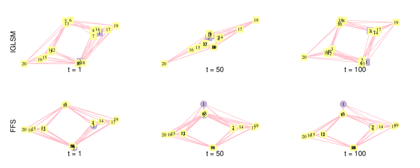
Figure 3: Snapshots of the estimated latent space for time points $1,50,100$, where only nodes $1,2$ transit and the rest stay static over time. Top row: IGLSM; bottom row: FFS. The estimated latent spaces for FFS are consistent across all time points, illustrating the long-range property of the proposed model.

On the other hand, inferring discrete structures from a continuous model through post-processing is a common objective in the literature (e.g., variable selection (Hahn and Carvalho,, 2015; Bashir et al.,, 2019) and rank estimation (Chakraborty et al.,, 2020)). Here, we consider a clustering analysis, which assigns cluster labels to the subjects $i=1,\ldots,n$, enabling the automatic grouping of subjects at a given time point $t$. In this article, we obtain cluster assignments using $K_{t}$-means after estimating the latent vectors, similar to spectral clustering, where $K$ means are obtained after acquiring latent vectors through spectral decomposition (Ng et al.,, 2001). Assume that the true latent vectors have only $K_{t}$ distinct rows. Then, given any obtained $\hat{\boldsymbol{U}}$, we can perform a $K_{t}$-means analysis on the row vectors of $\hat{\boldsymbol{U}}_{t}$:

$$(\hat{\boldsymbol{\Xi}}_{t},\hat{\boldsymbol{X}}_{t})=\operatorname*{argmin}_{\boldsymbol{\Xi}\in\mathbb{M}_{n,K_{t}},\boldsymbol{X}\in\mathbb{R}^{K_{t}\times d}}\|\boldsymbol{\Xi}\boldsymbol{X}-\hat{\boldsymbol{U}}_{t}\|_{F}^{2},$$

where $\mathbb{M}_{n,K_{t}}$ is the collection of membership matrices, each of which has exactly one $1$ and $K_{t}-1$ zeros in every row. The membership matrix $\hat{\boldsymbol{\Xi}}_{t}$ reveals the cluster assignments of subjects $i\in[n]$ at time $t$, and the row vectors of $\hat{\boldsymbol{X}}_{t}$ represent the estimated unique rows of latent factors at time $t$. Variants of $K_{t}$-means can also be applied, such as performing $K_{t}$-means after normalizing all row vectors (Von Luxburg,, 2007). The separation between the distinct rows of the truth significantly affects the performance of $K_{t}$-means.

3 Theoretical Analysis

In this section, we provide theoretical support for the proposed methodology. We only consider theoretical results for the matrix case, focusing on both the matrix factorization model (4) and the latent space model (5). The results should readily extend to the tensor case when the number of arms is fixed. First, we identify a suitable parameter space (8) reflecting the sparsity structure in the transitions for the decomposed low-rank matrices and obtain, in Theorem 3.1, a novel information-theoretic lower bound on the rate of recovery of $\mathcal{M}=\{\boldsymbol{M}_{t}\}_{t}$ under this parameter space. Then, in Theorem 3.2, we show that the rate of contraction of the fractional posterior, a variant of the usual posterior (see subsection 3.2 for details), matches the lower bound up to only a logarithmic factor, indicating the fractional posterior mean as a nearly rate-optimal estimator. Finally, we provide theoretical results for the post-processing, using dynamic network models as an example in Corollary 3.3 and Theorem 3.4. To simplify notation, we use $\boldsymbol{U},\boldsymbol{V}$ to denote $\boldsymbol{U}^{(1)}$ and $\boldsymbol{U}^{(2)}$ respectively. Denote $\varTheta=[\mathcal{U}^{\prime},\mathcal{V}^{\prime}]^{\prime},\mathcal{U}=[\boldsymbol{U}_{1},...,\boldsymbol{U}_{T}],\mathcal{V}=[\boldsymbol{V}_{1},...,\boldsymbol{V}_{T}],\boldsymbol{\Theta}_{t}=[\boldsymbol{U}_{t}^{\prime},\boldsymbol{V}_{t}^{\prime}]^{\prime}$ and $\boldsymbol{\theta}_{it}=\boldsymbol{u}_{it}$ if $i\in[n]$; $\boldsymbol{\theta}_{it}=\boldsymbol{v}_{(i-n)t}$ if $i=n+1,...,n+p$. Let $\boldsymbol{\theta}_{i\cdot}=[\boldsymbol{\theta}_{i1}^{\prime},...,\boldsymbol{\theta}^{\prime}_{iT}]^{\prime}$. Without ambiguity, we use the symbol $\varTheta,\boldsymbol{\Theta}_{t},\boldsymbol{\theta}_{it},\boldsymbol{\theta}_{i\cdot}$ for the symmetric case in equation (5) interchangeably with $\mathcal{U},\boldsymbol{U}_{t},\boldsymbol{u}_{it},\boldsymbol{u}_{i\cdot}$. For a vector $\boldsymbol{x}$, we use $\|\boldsymbol{x}\|_{2}$, $\|\boldsymbol{x}\|_{1}$, $\|\boldsymbol{x}\|_{\infty}$ to respectively represent its $\ell_{2}$, $\ell_{1}$ and $\ell_{\infty}$ norms, and $\boldsymbol{x}^{\prime}$ as its transpose. Let $\|\cdot\|_{F}$ denote the Frobenius norm of a matrix. Given sequences $a_{n}$ and $b_{n}$, we denote $a_{n}=O(b_{n})$ or $a_{n}\lesssim b_{n}$ if there exists a constant $C>0$ such that $a_{n}\leq Cb_{n}$ for all large enough $n$. Similarly, we define $a_{n}=\Omega(b_{n})$ or $a_{n}\gtrsim b_{n}$. In addition, let $a_{n}=o(b_{n}),a_{n}=\omega(b_{n})$ respectively correspond to $\lim_{n\rightarrow\infty}a_{n}/b_{n}=0$ and $\lim_{n\rightarrow\infty}b_{n}/a_{n}=0$ respectively.

3.1 Lower bound to the minimax risk

We first consider the following parameter space:

Double-sided Fusion (DSF):

$$\mbox{DSF}(s_{u},s_{v}):=\left\{\varTheta^{*}:\sum_{t=2}^{T}\sum_{i=1}^{n}\mathbbm{1}\{D\boldsymbol{u}^{*}_{it}\neq\boldsymbol{0}\}\leq s_{u},\,\sum_{t=2}^{T}\sum_{j=1}^{p}\mathbbm{1}\{D\boldsymbol{v}^{*}_{jt}\neq\boldsymbol{0}\}\leq s_{v}\right.$$ (8)

$$\left.\max_{i=1}^{n}\max_{t=1}^{T}\|\boldsymbol{u}_{it}\|_{2}\lesssim 1,\quad\max_{j=1}^{p}\max_{t=1}^{T}\|\boldsymbol{v}_{jt}\|_{2}\lesssim 1\right\}.$$

The sparsity constraint mentioned above implies that out of the total $n\times(T-1)$ transitions for the subjects of $\boldsymbol{U}$ and $p\times(T-1)$ transitions for the subjects of $\boldsymbol{V}$, only $s_{u}$ and $s_{v}$ transitions, respectively, are nonzero, while in the remaining cases, the latent vectors stay unchanged. Additionally, under the boundness assumption provided, for the Bernoulli likelihood, all the probabilities induced by the inner product $p_{u^{*}_{it},v^{*}_{jt}}:=1/\{1+\exp(-\boldsymbol{u}_{it}^{*^{\prime}}\boldsymbol{v}^{*}_{jt})\}$ are bounded away from $0$ and $1$. Sparsity levels $s_{u}$ and $s_{v}$ can be expressed as functions of $n,T$ and $p,T$, respectively. Next, we propose regularity conditions to further refine our understanding of the problem’s properties and behavior.

Assumption 1 (KL divergence regularity).

For any $\varTheta^{a}$, $\varTheta^{b}\in\mbox{DSF}(s_{u},s_{v})$, we assume the likelihood induced by $\boldsymbol{\Theta}_{t}^{a}$, $\boldsymbol{\Theta}_{t}^{b}$ for all $t\in[T]$ satisfies:

$$\max\left\{D_{KL}(p_{\boldsymbol{\Theta}_{t}^{a}},p_{\boldsymbol{\Theta}_{t}^{b}}),V_{2}(p_{\boldsymbol{\Theta}_{t}^{a}},p_{\boldsymbol{\Theta}_{t}^{b}})\right\}\lesssim\|\boldsymbol{U}_{t}^{a}\boldsymbol{V}_{t}^{a^{\prime}}-\boldsymbol{U}_{t}^{b}\boldsymbol{V}_{t}^{b^{\prime}}\|_{F}^{2},$$

where $D_{KL}(p_{\boldsymbol{\Theta}_{t}^{a}},p_{\boldsymbol{\Theta}_{t}^{b}})$ is the Kullback–Leibler (KL) divergence and $V_{2}(p_{\boldsymbol{\Theta}_{t}^{a}},p_{\boldsymbol{\Theta}_{t}^{b}})=$
$\int p_{\boldsymbol{\Theta}_{t}^{a}}\{\log(p_{\boldsymbol{\Theta}_{t}^{a}}/p_{\boldsymbol{\Theta}_{t}^{b}})^{2}\}dp_{\boldsymbol{\Theta}_{t}^{a}}$ is the second order moment of log-likelihood ratio between $p_{\boldsymbol{\Theta}_{t}^{a}}$ and $p_{\boldsymbol{\Theta}_{t}^{b}}$.

The assumption holds for many commonly used likelihood functions, like Gaussian and binary with true probabilities bounded away from $0$ and $1$. Given an estimator $\hat{\varTheta}$ of $\varTheta^{*}$, we consider the squared loss $\sum_{t=1}^{T}\|\hat{\boldsymbol{U}}_{t}\hat{\boldsymbol{V}}_{t}^{\prime}-\boldsymbol{U}^{*}_{t}\boldsymbol{V}^{*^{\prime}}_{t}\|_{F}^{2}/(npT)$ to formulate the minimax lower bound. Since $\boldsymbol{U}_{t},\boldsymbol{V}_{t}$ can only be identified up to rotation and scaling, the loss function is formulated in terms of the matrix products, which are rotation and scaling invariants. Then the following statement holds for the minimax lower bound:

Theorem 3.1.

Suppose the data generating process follows equation (4) and Assumption 1 holds, then suppose that $d$ is fixed. For large enough $n,p,T$, we have:

$$\begin{aligned} \inf_{\hat{\varTheta}}\sup_{\varTheta\in\mbox{DSF}(s_{u},s_{v})}\operatorname{\mathbf{E}}_{\varTheta}\left[\frac{1}{Tnp}\sum_{t=1}^{T}\|\hat{\boldsymbol{U}}_{t}\hat{\boldsymbol{V}}_{t}^{\prime}-\boldsymbol{U}^{*}_{t}\boldsymbol{V}^{*^{\prime}}_{t}\|_{F}^{2}\right]\\ \gtrsim\frac{1}{npT}\left\{{s_{u}\log\left(\frac{Tn}{s_{u}}\right)}+s_{v}\log\left(\frac{Tp}{s_{v}}\right)+n+p\right\}.\end{aligned}$$

Theorem 3.1 presents a novel result concerning the estimation of low-rank structured fused matrices with an information-theoretic lower bound. As far as we know, there are no similar results in the literature. We explicitly ignore the latent dimension $d$ in the bound by assuming it remains a fixed constant across time. The terms $s_{u}\log({Tn/s_{u}})$ and $s_{v}\log(Tp/s_{v})$ represent the selection errors for the fusion structure of $\mathcal{U}$ and $\mathcal{V}$, respectively. The term $(n+p)/(npT)$ identifies the initial estimation errors. Even in the extreme case that $s_{u}=s_{v}=0$, where all matrices are equal, it is still necessary to estimate $\boldsymbol{U}_{1}$ and $\boldsymbol{V}_{1}$. This matches the minimax lower bound $1+s\log(T/s)$ of the linear fused model (Fan and Guan,, 2018) with fusion sparsity $s$. On the other hand, in the dense case where $s_{u}\geq cnT$ and $s_{v}\geq cpT$ for some constant $c>0$, the lower bound is then $(n+p)/(np)$, which equates to estimating each low-rank mean matrix individually. If $n$ and $p$ are approximately equal, then both $\mathcal{U}$ and $\mathcal{V}$ must be structurally fused to deliver a measurable improvement in the lower bound. However, in the case of only a one-sided fusion structure, the lower bound may not even be improved from the error rate of the static case $(n+p)/(np)$. This highlights the importance of having two-sided fusion structures for better estimation performance.

3.2 Posterior contraction rate under FFS priors

To facilitate the theoretical analysis of the proposed model, we adopt the fractional posterior (Walker and Hjort,, 2001) framework, where the usual likelihood $P(\mathcal{Y}\mid\mathcal{U},\beta)$ is raised to a power $\alpha\in(0,1)$ to form a pseudo-likelihood $P_{\alpha}(\mathcal{Y}\mid\mathcal{U},\beta):=\left[P(\mathcal{Y}\mid\mathcal{U},\beta)\right]^{\alpha}$, leading to a fractional posterior $P_{\alpha}(\mathcal{U},\beta\mid\mathcal{Y})\propto P_{\alpha}(\mathcal{Y}\mid\mathcal{U},\beta)\,p(\mathcal{U})\,p(\beta)$. Such adaptation only requires minor changes in computation, while the theoretical analysis requires fewer conditions than the usual posterior (Bhattacharya et al.,, 2019). Similarly to the original posterior, the optimal convergence of a fractional posterior can imply a rate-optimal point estimator derived from the fractional posterior. We then need the following assumptions to establish results for the posterior convergence:

Assumption 2 (Likelihood regularity).

For any $0<\alpha<1$, and $\varTheta^{a}\,,\varTheta^{b}\in\mbox{DSF}(s_{u},s_{v})$, the $\alpha$-divergence induced by $\varTheta^{a}$, $\varTheta^{b}$ for all $t\in[T]$ satisfies:

$$D_{\alpha}(p_{\varTheta^{a}},p_{\varTheta^{b}})\gtrsim\|\boldsymbol{U}_{t}^{a}\boldsymbol{V}_{t}^{a^{\prime}}-\boldsymbol{U}_{t}^{b}\boldsymbol{V}_{t}^{b^{\prime}}\|_{F}^{2}.$$

Assumption 3 (Global prior).

For any $s_{i}\in[\max\{n,p\}]$, with $\log T=o(np),$ the global prior $g$ satisfies:

$$\log\left\{g(\tau_{i}^{\ast}<\tau<2\tau_{i}^{\ast})\right\}\gtrsim-s_{i}\log(npT),\quad\mbox{with}\quad\tau_{i}^{\ast}=\frac{s_{i}^{\frac{1}{2}}(\log(npT))^{\frac{1}{2}}}{(np)^{\frac{3}{2}}T^{\frac{5}{2}}}.$$

Similar to Assumption 1, Assumption 2 also holds for Gaussian and binary cases with true probabilities bounded away from $0$ and $1$, see Gil et al., (2013) for some detailed calculations. Assumption 3 requires that the global prior has a sufficient mass around proper small values. It can be satisfied by the priors $\tau\sim\mbox{Ca}^{+}(0,1)$ or $\tau^{2}\sim\mbox{Gamma}(a_{\tau},b_{\tau})$ with constants $a_{\tau},b_{\tau}$ as shown Proposition 8.1 in the appendix. Then we have the following main theorem:

Theorem 3.2.

Suppose the data generating process follows equation (4) and Assumptions 1, 2 and 3 hold. Then under the prior (3), if $\varTheta^{*}\in\mbox{DSF}(s_{u},s_{v})$ with $\log T=o(np)$ and $d$ is fixed. Denote $\epsilon_{n,p,T}=M\sqrt{(s_{u}+s_{v}+n+p)\log(npT)/npT}$ for some constant $M>0$. Then for large enough $n,p,T$, any $D\geq 2$ and $\eta>0$, with probability at least $1-2/\{(D-1+\eta)^{2}npT\epsilon_{n,p,T}^{2}\}$, we have

$$\Pi_{\alpha}\left\{\frac{1}{Tnp}\sum_{t=1}^{T}\|\boldsymbol{U}_{t}\boldsymbol{V}_{t}^{\prime}-\boldsymbol{U}^{*}_{t}\boldsymbol{V}^{*^{\prime}}_{t}\|_{F}^{2}\geq\frac{D+3\eta}{1-\alpha}\epsilon_{n,p,T}^{2}\mid\mathcal{Y}\right\}\leq e^{-\eta npT\epsilon_{n,p,T}^{2}}.$$

The above theorem indicates that the fractional posterior of the average estimation error can achieve the minimax lower bound with only a logarithmic factor when the true lists of row vectors of $\mathcal{U}$ and $\mathcal{V}$ are both group-wise fused. In the worst case, such a fusion type of lower bound cannot be matched by $\ell_{1}$ penalized regressions (Fan and Guan,, 2018). Therefore, theoretically, the proposed method is better than using $\ell_{1}$ regularization to introduce fusion structures. The proof of Theorem 3.2 is based on an $\ell_{1}$ type of prior concentration for the shrinkage prior shown in the supplementary material. The above theorem also demonstrates an advantage in comparison to the conditions required with the fusion model with only one variable. When there is only one variable of time $T$ with fusion sparsity $s$, then $s=o(T/\log(T))$ is required to make sure that the targeted rate $s\log T/T$ converges to zero. However, while the fusion structure holds for $np$ variables, the error rate for a subject with sparsity $s_{i}$ is $s_{i}\log(npT)/(npT)=s_{i}\log(np)/(npT)+s_{i}\log(T)/(npT)$. As long as the mild assumption $\log T=o(np)$ holds, the above rate converges to zero even if $s_{i}=T$, which is considerably more flexible since the successive differences of some subjects are therefore permitted to be non-sparse. In the next subsection, we use dynamic network models as an example to show the theoretical results for the post-processing, as described in Section 2.2, after obtaining the estimates.

3.3 Theoretical results for post-processing under dynamic network models

For dynamic network models, the estimation error in the inner product in Theorem 3.2 cannot directly imply the estimation of latent vectors that can be directly compared across time. To handle the issue, we study the recovery of latent vectors in the loss function (7). In particular, we divide the time $1,..,T$ into $T/k$ sets, where each set contains $k$ consecutive time points: ${(t-1)k+1,...,(t-1)k}_{t=1}^{T/k}$. We assume $\bar{t}=T/k$ is an integer for simplicity. We consider the comparison for latent space within each set of periods so that the maximal time gap is $k$ for each comparison. Then the following corollary characterizes the optimal estimation error of the estimator after sequential Procrustes rotations (6):

Corollary 3.3.

Suppose the Assumptions in Theorem 3.2 hold. In addition, assume that the smallest singular of $\boldsymbol{U}^{*}_{t}$, denoted as $\lambda_{t}$, satisfies $\lambda_{t}=\Omega(\sqrt{n})$ for $t\in[T]$. For the posterior means estimated $\hat{\boldsymbol{U}}_{t}$, after performing sequential Procrustes rotations (6) to obtain estimation $\hat{\boldsymbol{U}}^{o}_{1},...,\hat{\boldsymbol{U}}^{o}_{T}$, the average error for all windows satisfies

$$\frac{1}{nT}\sum_{t=1}^{\bar{t}}\inf_{\bar{\boldsymbol{O}}_{t,k}\in\mathbb{O}^{d\times d}}\sum_{k_{0}=1}^{k}\|\hat{\boldsymbol{U}}^{o}_{(t-1)k+k_{0}}-\boldsymbol{U}^{*}_{(t-1)k+k_{0}}\bar{\boldsymbol{O}}_{t,k}\|_{F}^{2}\lesssim\frac{(s+n)\log(nT)}{n^{2}T}$$

$$+\min\left\{\frac{k(s+n)\log(nT)}{n^{2}T},\frac{\log(nT)}{n}\right\}+\min\left\{\frac{sk(k-1)}{nT},\frac{s}{n},1\right\}.$$

An additional assumption characterizes the lower bound of the order of the smallest eigenvalue of the true latent vectors. The lower bound of the order $\sqrt{n}$ holds for many matrices. For example, for an $n\times d$ random matrix whose entries are i.i.d. distributed with zero mean and unit variance, the famous Bai-Yin’s law (Bai and Yin,, 2008) states that its smallest singular value is approximate $\sqrt{n}-\sqrt{d}$ (we refer to Vershynin, (2010) for more matrices with the same rate). When $k=1$, the error rate becomes the optimal estimation error in Theorem 3.2. When $k$ is a constant where the comparison is limited to adjacent ones, the average error for all windows converges to zero at rate $(s+n)\log(nT)/(n^{2}T)+s/(nT)$ as $n,T\rightarrow\infty$, leading to consistency as long as $s=o(nT)$. If the transition is extremely sparse $s=o(n)$, then one can simultaneously compare all the latent space for all time points of length $k=O(T)$. For the challenging case, where $s=o(nT)$, only constant time latent positions can be compared across time. In some special cases, the above error rate is not optimal. In supplementary subsection 8.9, we provide an improvement under a more stringent assumption of the true transitions. To our best knowledge, although Procrustes rotations have been popularly employed, there is no similar theoretical result to Corollary 3.3 that tries to quantitatively understand the possibility and limitations of long-term comparison of the estimated latent factors. Corollary 3.3 discusses the long-term properties of dynamic networks from a theoretical aspect.

Once the latent vectors have been obtained, $K$-means can be used to cluster the subjects. This is equivalent to detecting communities within networks. For any membership matrix $\boldsymbol{\Xi}$, the cluster membership of a subject $i$ is denoted by $g_{i}\in\{1,...,K\}$, which satisfies $\Xi{ig_{i}}=1$. Let $G_{k}(\Xi)=\{1\leq i\leq n:g_{i}=k\}$. We consider the following loss function to evaluate clustering accuracy

$$L(\hat{\boldsymbol{\Xi}},\boldsymbol{\Xi})=\min_{\boldsymbol{J}\in E_{K}}\|\hat{\boldsymbol{\Xi}}\boldsymbol{J}-\boldsymbol{\Xi}\|_{2,0},$$

which represents the number of misclustering subjects, where $E_{K}$ is the set of all $K\times K$ permutation matrix. Our next result concerns performing separate community detection for each network while improving the overall misclustering rate based on the network dependence structure.

Theorem 3.4.

Suppose the assumptions in Theorem 3.2 hold. In addition, assume that for $t\in[T]$, the truth $\boldsymbol{U}^{*}_{t}$ satisfies: 1. $\boldsymbol{U}^{*}_{t}$has $K_{t}$ distinct rows: $\boldsymbol{U}^{*}_{t}=\boldsymbol{\Xi}^{*}_{t}\boldsymbol{X}_{t}$, $\boldsymbol{\Xi}^{*}_{t}\in\mathbb{M}_{n,K_{t}}$ for some $K_{t}>0$ and $\boldsymbol{U}^{*}_{t}\in\mathbb{R}^{K_{t}\times d}$ is full rank; 2. The smallest singular value of $\boldsymbol{U}^{*}_{t}$, denoted as $\lambda_{t}$, satisfies $\lambda_{t}=\Omega(\sqrt{n})$; 3. Cluster separation: $\delta\leq\min_{i\neq j}\|\boldsymbol{u}^{*}_{it}-\boldsymbol{u}^{*}_{jt}\|_{2}$ for any $\boldsymbol{u}^{*}_{it}\neq\boldsymbol{u}^{*}_{jt}$, where $\delta>0$; 4. The minimal block size satisfies $\min_{i}|G_{i}(\boldsymbol{\Xi}^{*}_{t})|=\omega(\log(n)/\delta^{2})$.

Then after performing $K_{t}$-means for posterior means $\hat{\boldsymbol{U}}_{t}$ to obtain estimation of membership matrix $\hat{\boldsymbol{\Xi}}_{t}$, as $n,T\rightarrow\infty$, we have

$$\frac{1}{T}\sum_{t=1}^{T}L(\hat{\boldsymbol{\Xi}}_{t},\boldsymbol{\Xi}^{*}_{t})\lesssim\frac{(s+n)\log(nT)}{nT\delta^{2}}.$$

There exists a list of literature discussing community detection given a list of time-dependent networks under different settings (Liu et al.,, 2018; Pensky and Zhang,, 2019). Regarding assumptions in Theorem 3.4: Assumption 1 is prevalent in the literature on community detection for networks. Assumption 3 represents a minimum separation between different clusters, which can be a constant for many cases: For example, $\delta=1$ for a random matrix whose entries are i.i.d. binary distributed. Assumption 4 requires a minimum block size of the clusters. The usage of FFS is justified by cluster separation. Suppose at time $t$ we have $\boldsymbol{u}^{*}_{it}=\boldsymbol{u}^{*}_{jt}$ for subjects $i,j$. Then for time $t+1$, the subject $i$ move to another cluster while subject $j$ stay the same. Under the cluster separation condition, we have $\delta_{t+1}\leq\|\boldsymbol{u}^{*}_{j(t+1)}-\boldsymbol{u}^{*}_{i(t+1)}\|_{2}=\|\boldsymbol{u}^{*}_{j(t+1)}-\boldsymbol{u}^{*}_{jt}\|_{2}$, which requires the transitions of the subjects to be heterogeneous: either the transition is zero, or the transition is large. However, when smoothness-induced priors (e.g., Gaussian process priors) are adopted on the transitions, one assumes that the true difference satisfies some smoothness condition, which cannot adapt to the above heterogeneous requirement.

4 Computation

We present an efficient variational inference algorithm to approximate the posterior distribution under the FFS prior. The algorithm uses closed-form iterations of a coordinate-ascent method, which relies on the conditionally conjugate nature of the FFS prior as in the related literature (Loyal and Chen,, 2021; Zhao et al.,, 2022). Our variational inference algorithm targets the fractional posterior $p_{\alpha}(\mathcal{U},\beta\mid\mathbf{Y})$ defined in subsection 3.2 and aims to find the best approximation (in terms of KL divergence) from a structured mean-field variational (SMF) family $\Gamma$:

$$q(\mathcal{U},\beta)=\prod_{m=1}^{M}\prod_{i=1}^{n}q(\boldsymbol{u}^{(m)}_{i\cdot})q(\beta),$$ (9)

where $\boldsymbol{u}^{(m)}_{i\cdot}=[\boldsymbol{u}^{(m)^{\prime}}_{i1},...,\boldsymbol{u}^{(m)^{\prime}}_{iT}]^{\prime}$. The adopted SMF family accommodates the special structures of the $Td\times Td$ covariance matrix for $\boldsymbol{u}^{(m)}_{i\cdot}$, which includes the temporal dependence across time $t\in[T]$ and the group-wise dependence among components for the same subject $i$. The covariance of $\boldsymbol{u}^{(m)}_{i\cdot}$ is in a block tri-diagonal structure, which can be inverted efficiently (in $O(Td^{3})$ operations) using the Kalman smoothing framework. We first present the algorithm for the matrix case (4), and then extend it to the general tensor case (1) in Section 8.5 of the supplement.

The goal of the variational inference is

$$\begin{aligned} \hat{q}(\varTheta,\boldsymbol{\beta})&=\operatorname*{argmin}_{q(\varTheta,\boldsymbol{\beta})\in\Gamma}D_{KL}\left\{q(\varTheta,\boldsymbol{\beta})\mid\mid p_{\alpha}(\varTheta,\boldsymbol{\beta}\mid\mathcal{Y})\right\}=\operatorname*{argmin}_{q(\varTheta,\boldsymbol{\beta})\in\Gamma}-\operatorname{\mathbf{E}}_{q}\left\{\log\left(\frac{p_{\alpha}(\mathcal{Y},\varTheta,\boldsymbol{\beta})}{q(\varTheta,\beta)}\right)\right\},\end{aligned}$$

where the term $\operatorname{\mathbf{E}}_{q}\{\log(p_{\alpha}(\mathcal{Y},\varTheta,\beta)/q(\varTheta,\beta))\}$ is the evidence-lower bound (ELBO) and $p_{\alpha}(\varTheta,\boldsymbol{\beta}\mid\mathcal{Y})$ is the marginal posterior $p_{\alpha}(\varTheta,\boldsymbol{\beta}\mid\mathcal{Y})=\int p_{\alpha}(\varTheta,\boldsymbol{\beta},\boldsymbol{\Lambda},\boldsymbol{\sigma}_{0}\mid\mathcal{Y})d\boldsymbol{\Lambda}\,d\boldsymbol{\sigma}_{0}$. Recall that we denote $\varTheta=[\mathcal{U}^{\prime},\mathcal{V}^{\prime}]^{\prime},\boldsymbol{\Theta}_{t}=[\boldsymbol{U}_{t}^{\prime},\boldsymbol{V}_{t}^{\prime}]^{\prime}$ and $\boldsymbol{\theta}_{it}=\boldsymbol{u}_{it}$ if $i\in[n]$; $\boldsymbol{\theta}_{it}=\boldsymbol{v}_{(i-n)t}$ if $i=n+1,...,n+p$ for notation simplicity.

Furthermore, we adopt the variable augmentation that the square of the half-Cauchy distribution can be expressed as a mixture of Inverse-Gamma distributions (Neville et al.,, 2014): for $\lambda_{it}\sim\mbox{Ca}^{+}(0,1)$, we can write $\lambda_{it}^{2}\mid\eta_{it}\sim\mbox{IG}(\frac{1}{2},\frac{1}{\nu_{it}}),\quad\eta_{it}\sim\mbox{IG}(\frac{1}{2},1).$ Denote $\boldsymbol{H}=\{\eta_{it}\}_{i,t}$. Then the objective of KL minimization is as follows:

$$\hat{q}(\varTheta,\beta,\boldsymbol{H},\boldsymbol{\Lambda},\boldsymbol{\tau},\boldsymbol{\sigma}_{0}) =\operatorname*{argmin}_{q(\varTheta,\beta,\boldsymbol{H},\boldsymbol{\Lambda},\boldsymbol{\tau},\boldsymbol{\sigma}_{0})\in\Gamma}-\operatorname{\mathbf{E}}_{q}\left\{\log\left(\frac{p_{\alpha}(\mathcal{Y},\varTheta,\beta,\boldsymbol{H},\boldsymbol{\Lambda},\boldsymbol{\tau},\boldsymbol{\sigma}_{0})}{q(\varTheta,\beta,\boldsymbol{H},\boldsymbol{\Lambda},\boldsymbol{\tau},\boldsymbol{\sigma}_{0})}\right)\right\},$$

where now the SMF family is defined as:

$$q(\varTheta,\beta,\boldsymbol{H},\boldsymbol{\Lambda},\boldsymbol{\tau},\boldsymbol{\sigma}_{0})=\prod_{i=1}^{n+p}\left[q(\boldsymbol{\theta}_{i\cdot})q(\tau_{i})\prod_{t=1}^{T-1}\left\{q(\lambda_{it})q(\eta_{it})\right\}q(\sigma_{0i})\right]q(\beta).$$ (10)

The variational family defined in Equation (10) allows for updating $q(\eta_{it})$, $q(\lambda^{2}_{it})$, and $q(\sigma_{0i}^{2})$ in the inverse-Gamma conjugate family. Furthermore, $q(\boldsymbol{\tau})$ can be updated with a closed-form expression when the recommended half-Cauchy or Gamma prior is used. For likelihoods that are Gaussian or Bernoulli, updating $q(\beta)$ and $q(\boldsymbol{\theta}_{i\cdot})$ can be efficiently obtained through a message-passing framework. The derivations for these updates are provided in Section 8.3 of the supplementary material for completeness.

When applying CAVI algorithms to models with sparsity structures, the final accuracy depends heavily on the order of component-wise updating. Updating in a naive cyclical manner can lead to error accumulation, as noted in Huang et al., (2016). To prevent this, Ray and Szabó, (2021) proposed a prioritized updating approach for sparse regression. In our algorithm, we partition the subject-related components into different blocks based on the subject index, ${q(\boldsymbol{\theta}_{i\cdot}),q(\sigma_{0i}),q(\boldsymbol{\lambda}_{i\cdot}),q(\tau_{i}),q(\boldsymbol{\eta}_{i\cdot})},{i\in[n+p]}$, to avoid error accumulation. We update each block ${q(\boldsymbol{\theta}_{i\cdot}),q(\sigma_{0i}),q(\boldsymbol{\lambda}_{i\cdot}),q(\tau_{i}),q(\boldsymbol{\eta}_{i\cdot})}$ until convergence, and then move onto the next block. This block-wise updating strategy reduces cumulative error and converges quickly because the variational family (10) captures temporal dependence. In Section 8.4 of the supplement, we compare this algorithm with proximal gradient descent using an $\ell_{1}$ penalized objective function for each block (node fixed), and we extend the algorithm to tensor data in Section 8.5 of the supplement.

5 Data Analysis

5.1 Simulations

In this section, we perform simulations to show that the simultaneous low-rank and fusion structures can not be fully captured by some methods that only consider low-rankness or fusion structures. First, simulation cases are considered to compare with the following approaches: 1. SVD1: perform SVD to obtain the best rank $d$ approximation for matrices at each time; 2. SVD2: combine the observed matrices at the neighbor time together to perform a low-rank approximation: let $\tilde{\boldsymbol{Y}}_{t}=[\boldsymbol{Y}_{t-1},\boldsymbol{Y}_{t},\boldsymbol{Y}_{t+1}]$ ($\tilde{\boldsymbol{Y}}_{1}=[\boldsymbol{Y}_{1},\boldsymbol{Y}_{2}]$ and $\tilde{\boldsymbol{Y}}_{T}=[\boldsymbol{Y}_{T-1},\boldsymbol{Y}_{T}]$). We then perform low-rank approximation on $\tilde{\boldsymbol{Y}}_{t}$ where the rank is obtained by optimal hard thresholding (Gavish and Donoho,, 2014), and the estimator $\hat{\boldsymbol{Y}}_{t}$ is the corresponding sub-matrix of the low-rank estimator of $\tilde{\boldsymbol{Y}}_{t}$; 3. Flasso1: perform fused lasso to estimate each component over time separately; 4. Flasso2: perform fused lasso to estimate each component over time separately, then apply SVD to obtain the best rank $d$ approximation for each estimated matrix. SVD2 and Flasso2 are some modified approaches based on SVD and fused lasso to consider both low-rank and fusion structures in the final estimation, either based on a data argumentation or a two-step approach. Throughout all simulations, we fix the fractional power for the fractional likelihood defined in subsection 3.2 as $\alpha=0.95$, hyperparameters $a_{\sigma_{0}}=b_{\sigma_{0}}=1/2$. First, $25$ replicated data sets are generated from the following case: With $n,p=5,10,20$ with $n\geq p$, $\boldsymbol{u}^{(m)}_{i1}\sim\mathcal{N}(\boldsymbol{0},\mathbbm{I}),\quad i=1,...,n_{m},m=1,2$, $D\boldsymbol{u}^{(m)}_{it}=(0,0)^{\prime}\mbox{ with probability $\rho$ }$, $D\boldsymbol{u}^{(m)}_{it}=(-1,-1)^{\prime}\,\,\mbox{ with probability $(1-\rho)/2$}$, $D\boldsymbol{u}^{(m)}_{it}=(1,1)^{\prime}\,\,\mbox{ with probability $(1-\rho)/2$}$, and $Y_{ijt}\sim\mathcal{N}(\boldsymbol{u}^{(1)^{\prime}}_{it}\boldsymbol{u}^{(2)}_{jt},0.3^{2})\quad i\in[n_{1}];j\in[n_{2}];t\in[T].$ The above simulation corresponds to the example (4) introduced in the methodology section. The supplement provides two additional cases about the binary network and tensor models in subsection 8.2. We have $T=100,\,d=2,\,\rho=0.5,0.8,0.85,0.9,0.95,0.99$ across all cases. The expected number of effective parameters in the above simulations is $(n+p)(1-\rho)Td$ for the Gaussian factorization model. Simulation settings for FFS are as follows: In the Gaussian case, iterations are stopped when the difference between predictive root mean squared errors (RMSEs) in two consecutive cycles is less than $10^{-4}$. The estimated RMSE is also used to measure the discrepancy between the estimated and true latent distances. For the fused lasso, we use cross-validation to tune the hyperparameters. Note that all $np$ components are required to perform separately fused lasso with cross-validations.

Figure 4 provides numerical support for our theoretical results in multiple aspects. First, as $\rho$ increases, the estimation errors of FFS, Flasso1, Flasso2 and SVD2 decrease, whereas that of SVD barely changes. The reason is that SVD estimates observation matrices separately without considering temporal dependence, whereas other approaches can take advantage of dynamic dependence in the model. It can be seen that even though SVD2 can take into account partial temporal dependence, the exact fusion structure can not be captured, leading to large estimation errors than the proposed approach. Moreover, by comparing Flasso and Flasso 2, we can see that the simultaneously low-rank and fusion structure should be considered if the true data-generating process is constrained in that way. When the number of observations is sufficient, FFS consistently achieves lower RMSE than all other approaches. The more accurate estimation of FFS over Flasso and Flasso2 matches the theoretical results that our final estimators are near minimax optimal while the $\ell_{1}$ type of regularizations is not.

Finally, we perform simulations in the context of the dynamic latent space model (5) for dynamic networks introduced in the methodology section to demonstrate the effectiveness of FFS in clustering in the presence of sparse changes. We compare FFS priors to IGLSM, where we implement IGLSM via the same likelihood and variational inference framework, only changing the prior for the transition variance. The following setup is considered: Let $d=2,n=40,T=100$. The initial distribution of each component of the true latent vectors is uniformly sampled from $\{-2,2\}$, so that there are $2^{d}=4$ true clusters across all time: $(-2,-2),(-2,2),(2,-2),(2,2)$. Then we let all subjects transit with a probability $p$ each time, and switch uniformly to the other $3$ locations with a probability of $(1-p)/3$. Thus, the expected number of changes in cluster membership is $nT(1-p)$. We generate data according to the model $Y_{ij,t}\sim\mbox{Ber(logistic}(-2+\boldsymbol{u}_{it}^{\prime}\boldsymbol{u}_{jt})),i>j;Y_{ij,t}=Y_{ji,t},t\in[T],$ where the intercept $-2$ is to make sure the connection probabilities between cluster $(-2,2)$ and $(2,-2)$ are small enough. After obtaining the estimate of the latent vectors via variational means, we normalized all the latent subjects, performed Procrustes rotations (6) and then applied $K$-means with $4$ centers at each time independently. Finally, the average rand index over time between the true cluster and the estimated cluster determined by $K$-means is used to assess the accuracy of the clustering. Simulations are repeated $25$ times; the results are shown in Figure 5. According to the figure, FFS performs better than IGLSM except in the case $p=0.8,n=20$. This is because the sparsity assumption is somehow violated for the case $p=0.8,n=20$. Given the weak signals where the number of subjects $n$ is relatively small, the adaptive patterns between stopping and transition are hard to capture. In general, the more sparse the transitions, the better the performance in clustering, both for FFS and IGLSM, since sparsity introduces more dependence across time. In summary, FFS better captures the dependence introduced by sparsity in transitions than IGLSM.

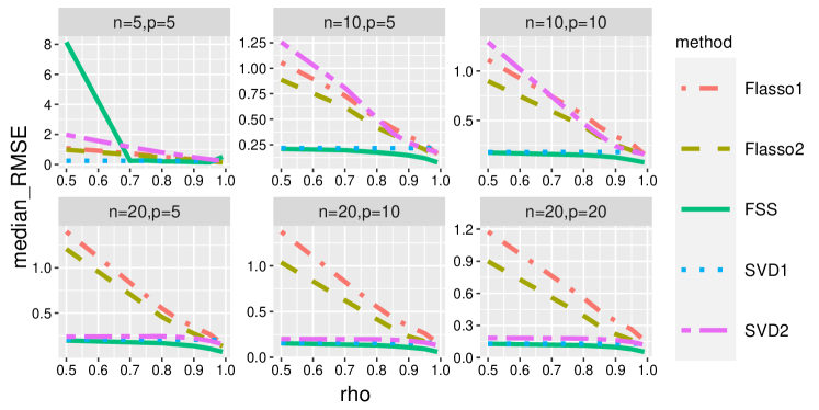
Figure 4: Performance comparison for Case 1 between FFS, SVD and Flasso. The measure is the median RMSE for the mean estimation of $\mathcal{M}$ across $25$ replicates. rho: $\rho$, the probability of remaining static for each time point and observation. FFS achieves lower RMSE than all other approaches when the number of observations is sufficient (except in the case $n=5,p=5$).

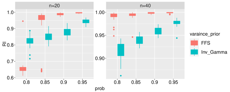
Figure 5: Boxplot comparing the performance of community detections between FFS and IGLSM. The measure is the median of means of the rand index calculated across $100$ time points using $K$-means over $25$ replications. RI: Rand index. $prob$: p. FFS performs no worse than IGLSM when the transitions are sparse or the number of subjects is sufficient (except $p=0.8$, $n=20$).

5.2 Real data analysis

Formal alliances data set:

Our methodology is applied to the formal alliances data set (Gibler, (2008), v4.1), which is a dynamic network data set recording all formal alliances (e.g., mutual defense pacts, non-aggression treaties, and ententes) among different nations between 1816 and 2012. An undirected edge between the two nations indicates that they formed a formal alliance in that year. We use a dynamic latent space model (5) under our methodology to analyze the data set. Studying the global military alliance networks can provide insight into the evolution of geopolitics and international relations across nations over the past two centuries. Visualizing the dynamic networks without a proper statistical model is challenging due to a large number of subjects ($n=180$ nations) and time points ($T=197$ years). For example, Park and Sohn, (2020) analyzed the data set with only selected years and subjects, both less than $10$. Our analysis aims to identify the significant historical events and countries that impacted the global alliance structure and provide a visual summary of these changes over time. While many territories changed during the period, we kept all the nations from the beginning to the end as long as they had at least one alliance at any given time. Therefore, the data set contains all subjects and all time points. Similar to the simulation subsection, we fix the fractional power $\alpha=0.95$ and hyperparameters $a_{\sigma_{0}}=b_{\sigma_{0}}=1/2$. We also choose $d=2$ for visualization purposes. Stopping criteria are taken as a difference between two consecutive training AUCs of not more than $0.01$. The estimate of the latent vectors is performed via variational means with Procrustes rotation (6). The figures and analyses are provided in the supplementary Section 8.1.

US domestic airline network during the COVID-19 pandemic:

We apply our proposed tensor models to analyze US domestic air transportation data from January 2018 to December 2021, obtained from the US Bureau of Transportation Statistics (US Bureau of Transportation Statistics,, 2022). The data is transformed into dynamic tensor-value observations, where the observed value for a carrier between two cities in a given month is represented as a binary value (0/1) indicating whether the carrier operated flights between the two cities during that month. Due to computational constraints, we limit the analysis to the 12 largest carriers and 100 cities with the highest number of flights, resulting in a time series tensor of size $100\times 100\times 12$ observed at $48$ time points with three modes: origin cities, destination cities, and carriers. One interesting aspect of this dynamic tensor data is its potential to track carriers’ reactions to the Covid-19 outbreak. Using the dynamic tensor-type low-rank model, our methodology can be applied to this task. We employ the FFS method with $d=2$ and a fixed fractional power of $\alpha=0.95$, along with hyperparameters $a_{\sigma_{0}}=b_{\sigma_{0}}=1/2$ similar to the simulation settings. We adopt a Gaussian likelihood with an $\mbox{IG}(1/2,1/2)$ prior on the variance instead of the Bernoulli one with logistics links, as the latter leads to unidentifiable estimations from the logistic links during the shut-down period when many nodes are isolated.

After estimation of the connection probabilities of the cities for different carriers, for example, let $\hat{P}_{\cdot,\cdot,i,t}$ be the estimated $100\times 100$ matrix of the connection probabilities of carrier $i$ at time $t$, we define the discrepancy measure as

$$d_{t1,t2,i}=\frac{\|\hat{P}_{\cdot,\cdot,i,t_{1}}-\hat{P}_{\cdot,\cdot,i,t_{2}}\|_{F}^{2}}{\|\hat{P}_{\cdot,\cdot,i,t_{1}}\|_{F}\|\hat{P}_{\cdot,\cdot,i,t_{2}}\|_{F}}.$$

The discrepancy measure $d_{t1,t2,i}$ is a measure of the relative change in the number of flights between two time periods $t_{1}$ and $t_{2}$ for a particular carrier $i$, where the normalization ensures that the measure is proportional to the relative change in the number of flights. The discrepancy measure has been normalized so that the maximum value across all carriers is equal to 1, resulting in Figure 6. Figure 6 illustrates a number of interesting phenomena. First, the period from April 2020 to July 2020 can be clearly identified as a shutdown period across all carriers, which is significantly different from other periods, implying that all carriers were affected by COVID-19 homogeneously during that time. Furthermore, the period from Aug. 2020 to Dec. 2021 behaves similarly to the pre-shutdown periods before March 2020. This is because the US Department of Transportation released a national strategy for the recovery of the US air transportation system in July 2020 (US Department of Transportation,, 2022), guiding the process of reviving the US air transportation industry. After the guidance was released, the US domestic airline industry entered the recovery stage. In addition, the magnitude of relative changes in the flights for different carriers is not uniform, with Southwest Airlines having the smallest changes among all airlines. In Sugishita et al., (2022), the specialty of Southwest Airlines with fewer variations in flights during the COVID outbreak was also found using a different analyzing approach.

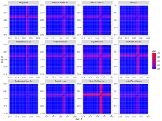
Figure 6: Heatmaps displaying the normalized $\ell_{2}$ distance matrices of the estimated connection probabilities for 12 US airline carriers from Jan. 2018 to Dec. 2021. The distances are normalized for each carrier by dividing all carriers’ largest distances. The period between April 2020 and July 2020 marked a significant shutdown phase across all carriers. In addition, Southwest Airlines exhibited less variation in the heatmap compared to the other 11 carriers.

6 Discussions

This paper examines dynamic latent variable models characterized by adaptively varying latent factors exhibiting negligible or significant changes over time. The proposed approach diverges from existing literature that typically considers changes in terms of Gaussian random walks or smooth transitions. We believe that the proposed FFS model can bring significant advantages when the inferential objective pertains to understanding the temporal evolution of cluster structures, as it preserves considerable separability between clusters. FFS enjoys strong theoretical support and efficient computation via a carefully structured mean-field variational inference algorithm, and we have illustrated its impressive performance in simulated and real datasets. Developing efficient MCMC algorithms toward full posterior exploration will be explored in future work. While the per-iteration complexity of MH-within-Gibbs-type algorithms should be similar with the proposed VI algorithm, mixing and convergence may be impacted by the strong posterior correlation between layers of latent variables.

7 Supplementary material

The supplementary material provides additional information to complement the main content. Section 8.1 presents figures and analyses related to the formal alliance data. Subsequent sections cover various topics: additional simulations in Section 8.2, algorithm details for SMF variational inference in Section 8.3, comparison of convergence for our algorithm within each block with others in Section 8.4, the algorithm for tensor data in Section 8.5, and proofs for the main theorems in Sections 8.6 to 8.10.

8 Appendix

8.1 Analysis for Formal alliances data set

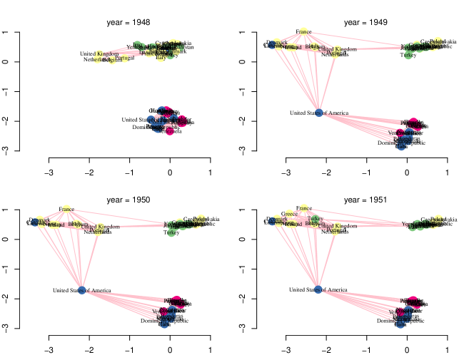
Figure 7: Latent space of world’s formal alliances for 1948 - 1951. The locations of countries’ names represent the corresponding subjects’ estimated locations after performing Procrustes rotation (6). Some selected labels are shown. Isolated subjects are not shown. Yellow, European countries; Red, South American countries; Blue, North American countries; Green, Asian countries; Green, African countries; Orange, Australian countries.

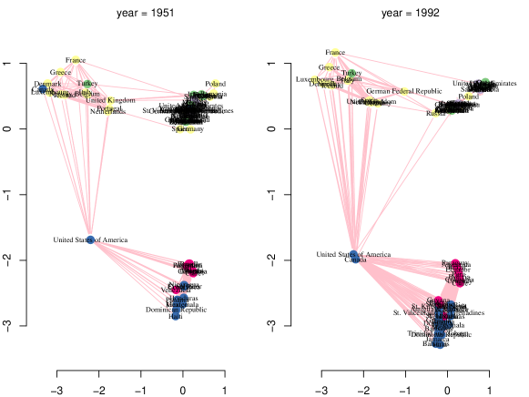
Figure 8: Latent space of world’s formal alliances for 1951 and 1992. The locations of countries’ names represent the corresponding subjects’ estimated locations after performing Procrustes rotation (6). Some selected labels are shown. Isolated subjects are not shown. Yellow, European countries; Rred, South American countries; Blue, North American countries; Green, Asian countries; Green, African countries; Orange, Australian countries.

Figure 7 in the supplement Section 8.1 displays the initial formation of the North Atlantic Treaty Organization (NATO). In 1948, the United States allied with several South American countries, as part of the Inter-American Treaty of Reciprocal Assistance. The graph shows that the United States was closely connected to these countries at that time. However, with the formation of NATO in 1949, the United States shifted its position and gained connections with NATO’s European members, demonstrating its strong influence in both America and Europe. Notably, from 1950 to 1951, Turkey also underwent a significant shift, moving from its proximity to Russia towards France, indicating its participation in NATO during 1951-1952. Figure 8 in the supplement Section 8.1 compares the estimated latent space between 1951 and 1992. Although there is a large time gap between the years, most nodes did not change their positions significantly, and the clustering structure remained similar. This reflects the stability of the world’s military structure during the Cold War based on the stopping property of the FFS model. In addition, some notable changes can be observed. For example, Canada gained several connections with South American countries, and its role became similar to that of the United States.

8.2 Additional simulations

8.2.1 Additional properties of FFS prior

In this section, we remark on the shrinkage effect of the FFS prior on the transitions at the scale of $\mathcal{M}_{t}$. Focusing on the Gaussian matrix factorization model with $d=2$, we examine the induced prior on the components of $D\mathcal{M}_{t}=\boldsymbol{U}_{t+1}\boldsymbol{V}_{t+1}^{\prime}-\boldsymbol{U}_{t}\boldsymbol{V}_{t}^{\prime}$ for different choices of the global parameter $\tau$. Given that $D\boldsymbol{u}_{it}$ and $D\boldsymbol{v}_{jt}$ are assigned group-wise shrinkage priors under FFS, the induced prior on the components of $D\mathcal{M}_{t}$ conditional on $\boldsymbol{u}_{i(t+1)},\boldsymbol{v}_{jt}$ can be expressed as a weighted sum of horseshoe-like priors. The summation and marginalization slightly decrease the mass assigned near the origin, which nevertheless can be adjusted by setting the global scale $\tau$ to a smaller value. To illustrate this, Figure 9 compares the shape of the FFS prior for different $\tau$ with the horseshoe prior on components of $D\mathcal{M}_{t}$ with $\tau=1$. According to the figure, the shrinkage effect towards $D\mathcal{M}_{t}$ is less pronounced than applying the usual horseshoe prior on elements of $D\mathcal{M}_{t}$ with the same $\tau$. We can, however, resolve this problem by using a smaller value of $\tau$. With $\tau=0.05$, the mass around zero is almost the same as that of the horseshoe prior applied directly to $D\mathcal{M}_{t}$ with $\tau=1$, while $\tau=0.01$ has even more mass around zero. Therefore, FFS priors can achieve a similar component-wise fusion shrinkage on mean matrices if the global prior on $\tau$ has a sufficient mass around zero. In particular, based on the details described in Assumption 3 in Section 3, the half-Cauchy prior $\tau^{(m)}_{i}\sim\mbox{Ca}^{+}(0,1)$ and Gamma prior $\tau_{i}^{(m)2}\sim\Gamma(a_{\tau},b_{\tau})$ can be adopted. As noted earlier, the application of the shrinkage on the latent factors instead of the components of $\mathcal{M}_{t}$ directly leads to a substantial reduction in the effective number of parameters.

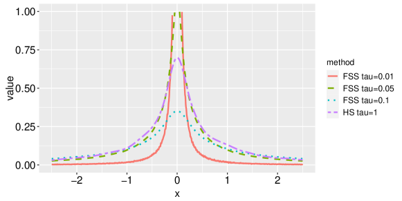
Figure 9: Density plot comparisons among marginal priors of $\boldsymbol{u}_{i(t+1)}^{\prime}\boldsymbol{v}_{j(t+1)}-\boldsymbol{u}^{\prime}_{it}\boldsymbol{v}_{jt}$ with different global parameters $\tau$ for FFS priors to the horseshoe prior (HS) component-wise on $D\mathcal{M}_{t}$ with the global parameter fixed at $\tau=1$. Value: values of fitted densities; $x$: $\boldsymbol{u}_{i(t+1)}^{\prime}\boldsymbol{v}_{j(t+1)}-\boldsymbol{u}^{\prime}_{it}\boldsymbol{v}_{jt}$. Small choices of $\tau$ in FFS priors can lead to similar marginal distributions with the HS prior applied directly to the component-wise differences.

We then provide some additional simulations in the binary network model and tensor model. The expected number of effective parameters is $n^{2}Td(1-\rho)$ for the binary network model, and $(n_{1}+n_{2}+n_{3})Td(1-\rho)$ for the tensor model. The piecewise change of binary and tensor cases is small to ensure that the absolute value of all latent vectors is bounded. We use the sample Pearson’s correlation coefficient (PCC) in the binary case to measure the discrepancy between the true and estimated probabilities. The stopping criterion is the difference between the training AUC (area under the curve) in two consecutive cycles not exceeding $0.01$.

Case 2, Binary network model:

$n=5,10,20,50$:

$$\boldsymbol{u}_{i1}\sim 0.5\mathcal{N}((1,0)^{\prime},\mathbbm{I})+0.5\mathcal{N}((-1,0)^{\prime},\mathbbm{I}),\quad i\in[n]$$

$$D\boldsymbol{u}_{it}=\begin{cases}(0,0)^{\prime}\,\,\mbox{ with probability $\rho$ }\\ (-0.25,-0.25)^{\prime}\,\,\mbox{ with probability $(1-\rho)/2$}\\ (0.25,0.25)^{\prime}\,\,\mbox{ with probability $(1-\rho)/2$}.\end{cases}\quad i\in[n];t=2,...,T$$

$$Y_{ijt}\sim\mbox{Ber(logistic}(\boldsymbol{u}_{it}^{\prime}\boldsymbol{u}_{jt}))\quad i>j;\quad Y_{ijt}=Y_{jit},t\in[T].$$

Case 3, Gaussian Tensor model:

$M=3$, $n_{1},n_{2},n_{3}=5,10$, $n_{1}\geq n_{2}\geq n_{3}$:

$$\boldsymbol{u}^{(m)}_{i1}\sim\mathcal{N}(\boldsymbol{0},\mathbbm{I}),\quad i\in[n_{m}],m=1,2,3$$

$$D\boldsymbol{u}^{(m)}_{it}=\begin{cases}(0,0)^{\prime}\,\,\mbox{ with probability $\rho$ }\quad\quad\quad m=1,2,3\\ (-0.25,-0.25)^{\prime}\,\,\mbox{ with probability $(1-\rho)/2$}\\ (0.25,0.25)^{\prime}\,\,\mbox{ with probability $(1-\rho)/2$},\end{cases}\quad i\in[n_{m}];t=2,...,T$$

$$\mathcal{Y}_{t}\sim\mathcal{N}(\sum_{l=1}^{d}\boldsymbol{u}^{(1)}_{t,l}\otimes\boldsymbol{u}^{(2)}_{t,l}\otimes\boldsymbol{u}^{(3)}_{t,l},0.3^{2})\quad i\in[n_{m}],m=1,2,3;\,t\in[T].$$

According to the simulation results from Table 1, when $\rho\geq 0.85$ increases, FFS, SVD and SVD2 improve estimation accuracy. The phenomenon occurs because the Bernoulli distribution has a smaller variance if the probabilities are close to zero or one. In addition, the initial distribution is generated from a mixture distribution with separate components that generate true probabilities close to zero or one. Consequently, if $\rho$ becomes larger, then the true binary responses for $t=2,...,T$ also tend to have probabilities close to $0$ or $1$, making it easier to obtain higher accuracy for the entire problem. Nevertheless, the proposed method still outperforms SVD and SVD2 in terms of PCC in almost all cases for $\rho\geq 0.8$. The results indicate that the proposed approach can benefit from the time dependence induced by fusion structure as $\rho$ increases, which cannot be ascribed to SVD and SVD2. When the sparsity assumption is violated with $\rho=0.5$, the proposed method is still comparable to SVD and SVD2. Next, Table 2 compares FFS with CP decomposition for tensor data generated in Case $3$. FFS performs better than CP across all simulation settings. Note that CP decomposition is optimized through alternating least squares, which is in a similar fashion to the CAVI algorithm. Therefore, both methods suffer from some bad local optimal induced by the alternating optimization mechanism. Therefore, the improvement in the estimation of FFS is simply because the fusion structure is taken into account.

Table 1: Performance comparison for binary cases between FFS and SVD. The measure is the median PCC for estimation of the connected probabilities.

$n$	Method	$\rho$
		0.5	0.8	0.85	0.9	0.95	0.99
5	FFS	0.909	0.867	0.920	0.959	0.984	0.990
	SVD	0.774	0.758	0.771	0.735	0.726	0.737
	SVD2	0.531	0.579	0.755	0.709	0.476	0.690
10	FFS	0.956	0.959	0.951	0.940	0.949	0.953
	SVD	0.864	0.833	0.833	0.829	0.876	0.889
	SVD2	0.829	0.819	0.844	0.852	0.884	0.881
20	FFS	0.973	0.980	0.985	0.985	0.994	0.999
	SVD	0.919	0.941	0.947	0.959	0.957	0.950
	SVD2	0.938	0.949	0.957	0.967	0.965	0.963
50	FFS	0.970	0.985	0.984	0.992	0.996	0.997
	SVD	0.934	0.967	0.936	0.970	0.973	0.973
	SVD2	0.972	0.975	0.960	0.978	0.979	0.981

Table 2: Performance comparison for tensor cases between FFS and CP decomposition. The measure is the median RMSE for estimation of the $\mathcal{M}$.

$(n_{1},n_{2},n_{3})$	Method	$\rho$
		0.5	0.8	0.85	0.9	0.95	0.99
(5 ,5 ,5)	FFS	0.132	0.119	0.119	0.121	0.127	0.113
	CP	0.187	0.147	0.153	0.145	0.148	0.143
(10 ,5 ,5)	FFS	0.114	0.107	0.102	0.106	0.103	0.104
	CP	0.213	0.127	0.132	0.117	0.117	0.121
(10 ,10 ,5)	FFS	0.093	0.088	0.087	0.082	0.081	0.074
	CP	0.159	0.121	0.111	0.092	0.092	0.092
(10 ,10 ,10)	FFS	0.073	0.068	0.069	0.067	0.067	0.065
	CP	0.192	0.072	0.073	0.071	0.071	0.072

8.2.2 Simulation settings for Figure 1

Let $d=2,n=10,T=100$. The initial distribution of each component of the true latent vectors is uniformly sampled from $\{(-1,-1)^{\prime},(-1,1)^{\prime},(1,-1)^{\prime},(1,1)^{\prime}\}$. The subjects $1$ and $2$ transit with probability $0.05$ at each time point, while the rest of the subjects stay static across all time. Data is then generated according to the model: $Y_{ijt}\sim\mbox{Ber(logistic}(2\boldsymbol{u}_{it}^{\prime}\boldsymbol{u}_{jt})),i>j;Y_{ijt}=Y_{jit},t\in[T]$.

8.3 CAVI algorithm

First, given $q(\varTheta)$, the updating of $q(\beta)$ is as follows:

$$q(\beta)\propto\exp[\operatorname{\mathbf{E}}_{-\beta}\{\log p_{\alpha}(\varTheta,\beta,\mathcal{Y})\}]\propto\exp[\operatorname{\mathbf{E}}_{\varTheta}\{\log P_{\alpha}(\mathcal{Y}\mid\varTheta,\beta)\}+\log p(\beta)],$$

which has a closed-form expression when the likelihood and priors are in a Gaussian form.

Given the above moment of $\lambda_{it}$, $\tau_{i}$ and $\sigma_{0i}$, the updating of $q(\boldsymbol{\theta}_{i\cdot})$ can be obtained through the message-passing framework: suppose $q(\beta)$, $q(\tau)$,$q(\sigma_{0})$ and $q_{j}(\boldsymbol{\theta}_{j\cdot}),\,j\neq i$ are given and the target is to update $q_{i}(\boldsymbol{\theta}_{i\cdot})$, we have:

$$q_{i}(\boldsymbol{\theta}_{i\cdot})\propto\exp\left[\operatorname{\mathbf{E}}_{-\boldsymbol{\theta}_{i\cdot}}\left\{{\sum_{t=1}^{T}\sum_{j\neq i,j=1}^{n}\{\log P_{\alpha}(Y_{ijt}\mid\boldsymbol{\theta}_{it},\boldsymbol{\theta}_{jt},\beta)\}}\right.\right.$$ (11)

$$\left.\left.+{\sum_{t=1}^{T-1}\log p(\boldsymbol{\theta}_{i(t+1)}\mid\boldsymbol{\theta}_{it},\lambda_{it})+\log p(\boldsymbol{\theta}_{i1}\mid\sigma_{0i})}\right\}\right],$$

where $\operatorname{\mathbf{E}}_{-\boldsymbol{\theta}_{it}}$ is the expectation taken with respect to the density $\big{[}\prod_{j\neq i}q_{j}(\boldsymbol{\theta}_{j\cdot})\big{]}q(\beta)q(\boldsymbol{\Lambda})q(\boldsymbol{\sigma}_{0})$.

We have the following factorial property for fractional joint distribution $p_{\alpha}(\mathcal{Y},\varTheta,\beta,\boldsymbol{H},\boldsymbol{\Lambda},\boldsymbol{\tau},\boldsymbol{\sigma}_{0})$:

$$\begin{aligned} &p_{\alpha}(\mathcal{Y},\varTheta,\beta,\boldsymbol{H},\boldsymbol{\Lambda},\boldsymbol{\tau},\boldsymbol{\sigma}_{0})\\ &\propto P_{\alpha}(\mathcal{Y}\mid\varTheta,\boldsymbol{\Lambda},\boldsymbol{\tau},\beta,\boldsymbol{\sigma}_{0},\boldsymbol{H})p(\varTheta\mid\boldsymbol{\Lambda},\boldsymbol{\tau},\boldsymbol{\sigma}_{0})p(\boldsymbol{\Lambda}\mid\boldsymbol{H})p(\boldsymbol{H})p(\beta)p(\boldsymbol{\tau})\\ &=\prod_{i=1}^{n}\left\{\prod_{t=1}^{T-1}p(\boldsymbol{\theta}_{i(t+1)}\mid\boldsymbol{\theta}_{it},\lambda_{it},\tau_{i})p(\lambda_{it}\mid\eta_{it})p(\eta_{it})p(\boldsymbol{\theta}_{i1}\mid\sigma_{0i})\right\}p(\beta)p(\tau_{i})\\ &\times\prod_{t=1}^{T}\prod_{1\leq i\neq j\leq n}P_{\alpha}(Y_{ijt}\mid\boldsymbol{\theta}_{it},\boldsymbol{\theta}_{jt},\beta),\end{aligned}$$ (12)

with $p(\boldsymbol{\theta}_{i(t+1)}\mid\boldsymbol{\theta}_{it},\lambda_{it},\tau_{i})\propto\exp(-\|\boldsymbol{\theta}_{i(t+1)}-\boldsymbol{\theta}_{it}\|_{2}^{2}/(2\tau_{i}^{2}\lambda^{2}_{it}))$ for $t\in[T-1]$.

By the scheme of CAVI, given the distributions $q(\varTheta),q(\beta)$, we have updatings of $\lambda_{it},\eta_{it},\sigma_{0i}$:

$$\hat{q}(\lambda_{it},\eta_{it},\sigma_{0i}) \propto\exp[\operatorname{\mathbf{E}}_{-\lambda_{it},\eta_{it},\sigma_{0i}}\{\log p_{\alpha}(\mathcal{Y},\varTheta,\beta,\boldsymbol{H},\boldsymbol{\Lambda},\boldsymbol{\tau},\boldsymbol{\sigma}_{0})\}]$$

$$\propto\exp[\operatorname{\mathbf{E}}_{-\lambda_{it},\eta_{it},\sigma_{0i}}\{\log P(\varTheta\mid\boldsymbol{\sigma}_{0},\boldsymbol{\Lambda})+\log P(\boldsymbol{\Lambda}\mid\boldsymbol{H})+\log P(\boldsymbol{H})+\log p(\boldsymbol{\sigma}_{0})\}]$$

$$\propto\exp\left[-\frac{d+3}{2}\log(\lambda_{it}^{2})-\operatorname{\mathbf{E}}_{\boldsymbol{\theta}_{i\cdot}}\left\{\frac{\|\boldsymbol{\theta}_{it}-\boldsymbol{\theta}_{i(t+1)}\|^{2}}{2\tau_{i}^{2}\lambda_{it}^{2}}\right\}-2\log(\eta_{it}^{2})-\frac{1}{\eta_{it}\lambda^{2}_{it}}-\frac{1}{\eta_{it}}\right.$$

$$\left.-\operatorname{\mathbf{E}}_{x_{i1}}\left(\frac{\|\boldsymbol{\theta}_{i1}\|^{2}_{2}}{2\sigma^{2}_{0i}}\right)-\left(\frac{d}{2}+a_{\sigma_{0}}+1\right)\log(\sigma_{0}^{2})-\frac{b_{\sigma_{0}}}{\sigma_{0i}^{2}}\right].$$

Therefore, we have

$$\eta_{it}^{(new)} \sim\mbox{IG}\left(1,1+\mu_{1/\lambda_{it}^{2}}\right);$$ (13)

$$\lambda_{it}^{2(new)} \sim\mbox{IG}\left(\frac{d+1}{2},\mu_{1/\eta_{it}}+\operatorname{\mathbf{E}}_{\boldsymbol{\theta}_{it},\boldsymbol{\theta}_{i(t+1)}}\left[\frac{\|\boldsymbol{\theta}_{it}-\boldsymbol{\theta}_{i(t+1)}\|_{2}^{2}}{2\tau_{i}^{2}}\right]\right);$$

$$\sigma_{0i}^{2(new)} \sim\mbox{IG}\left(\frac{nd+a_{\sigma_{0}}}{2},\frac{\operatorname{\mathbf{E}}_{q(\boldsymbol{\theta}_{i1})}(\|\boldsymbol{\theta}_{i1}\|_{2}^{2})+2b_{\sigma_{0}}}{2}\right),$$

where $\mu_{1/\lambda_{it}^{2}}=\operatorname{\mathbf{E}}_{q(\lambda_{it})}(1/\lambda_{it}^{2})$ and $\mu_{1/\eta_{it}}=\operatorname{\mathbf{E}}_{q(\eta_{it})}(1/\eta_{it})$. Note that the key moment has a closed-form expression in terms of the parameters: $a\sim\mbox{IG}(\alpha,\beta)$, $\operatorname{\mathbf{E}}(1/a)=\alpha/\beta$.

Given the equation (11), note that $q_{i}(\boldsymbol{\theta}_{i\cdot})$ has the following form:

$$q_{i}(\boldsymbol{\theta}_{i\cdot})=q_{i1}(\boldsymbol{\theta}_{i1})\prod_{t=1}^{T-1}q(\boldsymbol{\theta}_{i(t+1)}\mid q(\boldsymbol{\theta}_{it}))=\prod_{t=1}^{T-1}\frac{q_{it,i(t+1)}(\boldsymbol{\theta}_{it},\boldsymbol{\theta}_{i(t+1)})}{q_{it}(\boldsymbol{\theta}_{it})q_{i(t+1)}(\boldsymbol{\theta}_{i(t+1)})}\prod_{t=1}^{T}q_{it}(\boldsymbol{\theta}_{it}).$$ (14)

It follows that the graph of random variable $\boldsymbol{\theta}_{i\cdot}$ is structured by a chain from $\boldsymbol{\theta}_{i1}$ to $\boldsymbol{\theta}_{iT}$. Due to the above structure (14), the computation of $q_{i}(\boldsymbol{\theta}_{i\cdot})$ given the rest densities can be carried out efficiently in a message-passing manner. In particular, the message-passing algorithm involves computing all the unary marginals $\{q_{it}\}$ and binary marginals $\{q_{it,i(t+1)}\}$, which in turn help to update scales in closed forms (13).

When Gaussian likelihood is adopted:

$$P_{\alpha}(\mathcal{Y}\mid\varTheta,\beta)=\prod_{t=1}^{T}\prod_{1\leq i\leq n,1\neq j\leq p}\frac{1}{\sqrt{2\pi}\sigma}\exp\left[-\alpha\frac{\{Y_{ijt}-\boldsymbol{u}_{it}^{\prime}\boldsymbol{v}_{jt}\}^{2}}{2\sigma^{2}}\right].$$

where $\sigma$ is the $\beta$ in the previous general setting, the MP updating can be implemented in the framework of Gaussian belief propagation networks, where the mean and covariance of the new update of variational distribution can be calculated by Gaussian conjugate and marginalization using the Schur complement. In addition, the updating of $\sigma$ can also be obtained in the closed forms via inverse-gamma conjugacy.

For the Bernoulli likelihood:

$$P_{\alpha}(Y_{ijt}\mid\boldsymbol{u}_{it},\boldsymbol{v}_{jt})=\exp[\alpha Y_{ijt}(\boldsymbol{u}_{it}^{\prime}\boldsymbol{v}_{jt})-\alpha\log\{1+\exp(\boldsymbol{u}_{it}^{\prime}\boldsymbol{v}_{jt})\}].$$

The tangent transform approach proposed by Jaakkola and Jordan, (2000) is applied in the present context to obtain closed-form updates.

By introducing $\Xi=\{\xi_{ijt}:i,j=1,...,n,t\in[T]\}$ with $A(\xi_{ijt})=-\mbox{tanh}(\xi_{ijt}/2)/(4\xi_{ijt})$ and $C(\xi_{ijt})=\xi_{ijt}/2-\log(1+\exp(\xi_{ijt}))+\xi_{ijt}\mbox{tanh}(\xi_{ijt}/2)/(4\xi_{ijt})$ for any $\xi_{ijt}$, the following lower bound on $P_{\alpha}(Y_{ijt}\mid\boldsymbol{u}_{it},\boldsymbol{u}_{jt},\beta)$ holds:

$$\underline{P}_{\alpha}(Y_{ijt}\mid\boldsymbol{u}_{it},\boldsymbol{v}_{jt};\xi_{ijt})=\exp\left[\alpha A(\xi_{ijt})(\boldsymbol{u}_{it}^{\prime}\boldsymbol{v}_{jt})^{2}+\alpha\left(Y_{ijt}-\frac{1}{2}\right)(\boldsymbol{u}_{it}^{\prime}\boldsymbol{v}_{jt})+\alpha C(\xi_{ijt})\right].$$

The likelihood $P_{\alpha}(Y_{ijt}\mid\boldsymbol{u}_{it},\boldsymbol{u}_{jt})$ is replaced by its lower bound $\underline{P}_{\alpha}(Y_{ijt}\mid\boldsymbol{u}_{it},\boldsymbol{v}_{jt};\xi_{ijt})$, where the updating of $\varTheta$ in the Gaussian conjugate framework can be performed. After updating all the variational densities, $\xi_{ijt}$ is optimized based on EM algorithm according to Jaakkola and Jordan, (2000): $\xi^{(new)}_{ijt}=\operatorname{\mathbf{E}}_{q(\varTheta)}\{(\boldsymbol{u}_{it}^{\prime}\boldsymbol{v}_{jt})^{2}\}$. To summarize, for Gaussian or Bernoulli likelihoods, the proposed variational framework allows all updating in the Gaussian conjugate paradigm by assuming only independent relationships between different subjects within the variational family.

8.4 Comparison of the MP algorithm to proximal gradient for $\ell_{1}$ penalized trend filtering

Due to the fact that the variational family (10) captures the temporal dependence, the computation of $q(\boldsymbol{\theta}_{\cdot})$ given the rest densities can be carried out in a message-passing manner. The proposed VI algorithm converges faster than the proximal gradient descent algorithm for $\ell_{1}$ regularized trend filtering problem without increasing the complexity of computation and storage per iteration due to the fact that message-passing utilizes the banded (block tri-diagonal) structure of the second-order moments, which can be inverted at an $O(Td^{3})$ cost. Figure 10 provides a simulation example by comparing our convergence in iterations between the proposed VI approach and the proximal and accelerated proximal gradient descent for a trend-filtering problem with $\ell_{1}$ regularization for $d=1$.

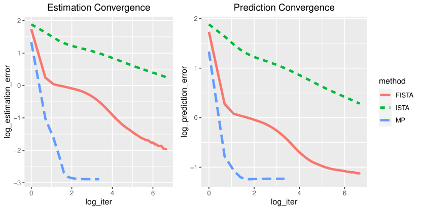
Figure 10: Comparison in iterations between message passing variational inference under proposed prior vs. proximal (ISTA) and accelerated proximal gradient descent (FISTA) under $\ell_{1}$ regularized trend filter problem. The hyperparameter $\tau$ of FFS are assigned with a fixed value to avoid model selection for fair comparison.

8.5 Computation for tensor data

For tensor data, the shrinkage priors are similarly applied on the transitions $\boldsymbol{u}^{(m)}_{it}\mid\boldsymbol{u}^{(m)}_{i(t-1)}\sim\mathcal{N}(\boldsymbol{u}^{(m)}_{i(t-1)},\tau^{(m)2}_{i}\lambda^{(m)2}_{it})$, and the SMF family is similarly defined:

$$q(\mathcal{U},\beta,\boldsymbol{H},\boldsymbol{\Lambda},\boldsymbol{\tau},\boldsymbol{\sigma}_{0})=\prod_{m=1}^{m}\prod_{i=1}^{n_{m}}\left[q(\boldsymbol{u}^{(m)}_{i\cdot})q(\tau^{(m)}_{i})\prod_{t=1}^{T-1}\left\{q(\lambda^{(m)}_{it})q(\eta^{(m)}_{it})\right\}q(\sigma^{(m)}_{0i})\right]q(\beta).$$

Then the extension from matrix to tensor is based on the tensor unfolding technique, as in Hoff, (2011) and Zhou et al., (2013). Tensor unfolding allows the components of the mean to be expressed as inner products of a targeted vector and component-wise products of some other vectors, which is fortunate to be compatible with the alternating updatings of the SMF variational family. Note that when we assume $\mathcal{M}_{t}$ defined as equation (1), we have the mode-$m$ unfolding:

$$\mathcal{M}_{t,(m)}=\left\{\boldsymbol{U}_{t}^{(M)}\odot\ldots\boldsymbol{U}_{t}^{(m+1)}\odot\boldsymbol{U}_{t}^{(m-1)}\odot\ldots\boldsymbol{U}_{t}^{(1)}\right\}\boldsymbol{U}_{t}^{(m)^{\prime}},$$

where $\odot$ is the Khatri-Rao product: $\boldsymbol{A}\odot\boldsymbol{B}=[\boldsymbol{a}_{1}\otimes\boldsymbol{b}_{1},...,\boldsymbol{a}_{K}\otimes\boldsymbol{b}_{K}]$ for $\boldsymbol{A}=[\boldsymbol{a}_{1},...,\boldsymbol{a}_{K}]\in\mathbb{R}^{I\times K}$ and $\boldsymbol{B}=[\boldsymbol{b}_{1},...,\boldsymbol{b}_{K}]\in\mathbb{R}^{J\times K}$. Therefore, the components of $\mathcal{M}_{t,(m)}$ equal inner products between row vectors of $\boldsymbol{U}_{t}^{(M)}\odot\ldots\boldsymbol{U}_{t}^{(m+1)}\odot\boldsymbol{U}_{t}^{(m-1)}\odot\ldots\boldsymbol{U}_{t}^{(1)}$ and $\boldsymbol{U}_{t}^{(m)}$. In particular, for $\{i_{m}\in[n_{m}]\}_{m}$, we have

$$\left\{\boldsymbol{u}_{i_{M}t}^{(M)}\circ\ldots\boldsymbol{u}_{i_{m+1}t}^{(m+1)}\circ\boldsymbol{u}_{i_{m-1}t}^{(m-1)}\circ\ldots\circ\boldsymbol{u}_{i_{1}t}^{(1)}\right\}^{\prime}\boldsymbol{u}^{(m)}_{jt}=\mathcal{[}M_{t,(m)}]_{i,j}$$

with $i=(i_{M}-1)(\prod_{j=1,j\neq M}^{M-1}n_{j})+...+(i_{m+1}-1)(\prod_{j=1}^{m-1}n_{j})+(i_{m-1}-1)(\prod_{j=1}^{m-2}n_{j})+...+i_{1}$, where $\circ$ is the Hadamard (element-wise) product. In the CAVI algorithm for the SMF family, when all the targeted row vectors follow Gaussian distributions, calculating the first and second moments of $\boldsymbol{u}_{i_{M}t}^{(M)}\circ\ldots\boldsymbol{u}_{i_{m+1}t}^{(m+1)}\circ\boldsymbol{u}_{i_{m-1}t}^{(m-1)}\circ\ldots\circ\boldsymbol{u}_{i_{1}t}^{(1)}$ is necessary to update a new mean and covariance for the distribution of $\boldsymbol{u}_{i_{m}t}^{(m)}$. For the component-wise product above, the first moment is straightforward, and the following lemma can be used to calculate the second moment sequentially:

Lemma 8.1.

Suppose $\boldsymbol{a}\sim\mathcal{N}(\boldsymbol{\mu},\boldsymbol{\Sigma})$ and $\boldsymbol{\Xi}$ is a positive definite matrix. Let $\boldsymbol{D}(\boldsymbol{a})=diag(\boldsymbol{a})$, then we have

$$\operatorname{\mathbf{E}}(\boldsymbol{D}(\boldsymbol{a})\boldsymbol{\Xi}\boldsymbol{D}(\boldsymbol{a}))=\boldsymbol{D}(\boldsymbol{\mu})\boldsymbol{\Xi}\boldsymbol{D}(\boldsymbol{\mu})+\boldsymbol{\Xi}\circ\boldsymbol{\Sigma},$$

With the lemma, given $\operatorname{\mathbf{E}}(\boldsymbol{a}\boldsymbol{a}^{\prime})$ and $\boldsymbol{b}\sim\mathcal{N}(\boldsymbol{\mu}_{b},\boldsymbol{\Sigma}_{b})$, we can first calculate $\operatorname{\mathbf{E}}((\boldsymbol{b}\circ\boldsymbol{a})(\boldsymbol{b}\circ\boldsymbol{a})^{\prime})=\operatorname{\mathbf{E}}(\boldsymbol{D}(\boldsymbol{b})\boldsymbol{a}\boldsymbol{a}^{\prime}\boldsymbol{D}(\boldsymbol{b}))$. Then $\operatorname{\mathbf{E}}((\boldsymbol{c}\circ\boldsymbol{b}\circ\boldsymbol{a})(\boldsymbol{c}\circ\boldsymbol{b}\circ\boldsymbol{a})^{\prime})$ can also be calculated sequentially with another normal distributed vector $\boldsymbol{c}$. A similar technique can also be applied when additional auxiliary variables are estimated using additional MF factorization. For example, to estimate the variance of the noise of a Gaussian tensor model $\sigma$, commonly used inverse-Gamma conjugate updates can be applied together within the MF framework, then the necessary term $\operatorname{\mathbf{E}}_{q}\{\sum_{t=1}^{T}(\mathcal{Y}_{t}-\mathcal{M}_{t})^{2}\}$ can also be computed through the above strategy.

8.6 Proof of Theorem 3.1

Proof.

For $\varTheta^{a}=[\mathcal{U}^{a^{\prime}},\mathcal{V}^{a^{\prime}}]^{\prime}$ and $\varTheta^{b}=[\mathcal{U}^{b^{\prime}},\mathcal{V}^{b^{\prime}}]^{\prime}$, let

$$d^{2}(\varTheta^{a},\varTheta^{b})=\sum_{t=1}^{T}\|\boldsymbol{U}^{a}_{t}\boldsymbol{V}^{a^{\prime}}_{t}-\boldsymbol{U}^{b}_{t}\boldsymbol{V}^{b^{\prime}}_{t}\|_{F}^{2},$$

and

$$d_{0}^{2}(\boldsymbol{U}^{a}_{t}\boldsymbol{V}^{a^{\prime}}_{t},\boldsymbol{U}^{b}_{t}\boldsymbol{V}^{b^{\prime}}_{t})=\|\boldsymbol{U}^{a}_{t}\boldsymbol{V}^{a^{\prime}}_{t}-\boldsymbol{U}^{b}_{t}\boldsymbol{V}^{b^{\prime}}_{t}\|_{F}^{2}.$$

The hypothesis set is constructed such that all elements are sufficiently distinct and the cardinality of the set can be constrained.

8.6.1 Asymmetric case:

To obtain the final bound for the asymmetric case, we use an alternative strategy. Initially, we fix $\mathcal{V}$ and select a suitable parameter space for $\mathcal{U}$ to obtain a rate of the lower bound; we then fix $\mathcal{U}$ and construct a hypothesis space for $\mathcal{V}$ to obtain a second lower bound. The final rate of the lower bound should be the sum of the two.

As a first step, we should first obtain a sparse Varshamov-Gilbert bound in Lemma 8.2 under Hamming distance for the low-rank subset construction:

Lemma 8.2 (Lemma 4.10 in Massart, (2007)).

Let $\Omega=\{0,1\}^{n}$ and $1\leq n_{0}\leq n/4$. Then there exists a subset $\{\boldsymbol{w}^{(1)},...,\boldsymbol{w}^{(M)}\}\subset\Omega$ such that

1. $\|\boldsymbol{w}^{(i)}\|_{0}=n_{0}$ for all $1\leq i\leq M$;

2. $\|\boldsymbol{w}^{(i)}-\boldsymbol{w}^{(j)}\|_{0}\geq n_{0}/2$ for $0\leq i\neq j\leq M$;

3. $\log M\geq cn_{0}\log(n/n_{0})$ with $c\geq 0.233$.

We construct the following case according to Lemma 8.2 (the construction holds under $n-d+1\geq 4$). For each $\boldsymbol{w}$, we can construct an $n\times d$ matrix and a $p\times d$ matrix as follows:

$$\boldsymbol{U}^{w}=\begin{bmatrix}\epsilon\boldsymbol{w}&\boldsymbol{0}\\ \boldsymbol{0}&\boldsymbol{I}_{d-1}\end{bmatrix}\quad\mbox{with}\quad w\in\Omega_{M};\quad\boldsymbol{V}^{0}=\begin{bmatrix}\boldsymbol{1}_{p-d+1}&\boldsymbol{0}\\ \boldsymbol{0}&\boldsymbol{I}_{d-1}\end{bmatrix},$$

which gives

$$\boldsymbol{U}^{w}\boldsymbol{V}^{0^{\prime}}=\begin{bmatrix}\epsilon\boldsymbol{w}\boldsymbol{1}^{\prime}&\boldsymbol{0}\\ \boldsymbol{0}&\boldsymbol{I}_{d-1}\end{bmatrix}.$$

The effect of this construction is that: for different $\boldsymbol{w}_{1},\boldsymbol{w}_{2}\in\Omega_{M}$, since $n_{0}/2\leq\|\boldsymbol{w}_{1}-\boldsymbol{w}_{2}\|_{0}\leq 2n_{0}$ and $\|\boldsymbol{V}^{0}\|_{F}\leq\sqrt{p}$, we have

$$d_{0}(\boldsymbol{U}^{w_{1}}\boldsymbol{V}^{0^{\prime}},\boldsymbol{U}^{w_{2}}\boldsymbol{V}^{0^{\prime}})\leq\|\boldsymbol{U}^{w_{1}}-\boldsymbol{U}^{w_{2}}\|_{F}\|\boldsymbol{V}^{0}\|_{F}=\sqrt{n}\epsilon\|\boldsymbol{w}_{1}-\boldsymbol{w}_{2}\|_{2}\leq\sqrt{{2pn_{0}}}\epsilon.$$

In addition, note that

$$d^{2}_{0}(\boldsymbol{U}^{w_{1}}\boldsymbol{V}^{0^{\prime}},\boldsymbol{U}^{w_{2}}\boldsymbol{V}^{0^{\prime}})=(p-d-1)\epsilon^{2}\sum_{i=1}^{n_{0}}(w_{1i}-w_{2i})^{2}\geq\frac{n_{0}(p-d-1)\epsilon^{2}}{2}.$$

Let

$$\boldsymbol{U}^{0}=\begin{bmatrix}\boldsymbol{0}&\boldsymbol{0}\\ \boldsymbol{0}&\boldsymbol{I}_{d-1}\end{bmatrix}$$

$\mathcal{U}^{0}=[\boldsymbol{U}^{0},...,\boldsymbol{U}^{0}]$, $\mathcal{V}^{0}=[\boldsymbol{V}^{0},...,\boldsymbol{V}^{0}]$ and $\varTheta^{0}=[\mathcal{U}^{0^{\prime}},\mathcal{V}^{0^{\prime}}]^{\prime}.$

We need the above Varshamov-Gilbert Bound 8.2 again to introduce another binary coding:

Let $\Omega_{r}=\{\boldsymbol{\phi}^{(1)},...,\boldsymbol{\phi}^{(M_{0})}\}\subset\{0,1\}^{T}$, such that $\|\boldsymbol{\phi}^{(i)}\|_{0}=t_{0}$ for all $1\leq i\leq M_{0}$ and $\|\boldsymbol{\phi}^{(i)}-\boldsymbol{\phi}^{(j)}\|_{0}\geq t_{0}/2$ for $0\leq i<j\leq M_{0}$ with $\log M_{0}\geq ct_{0}\log(T/t_{0})$ with $c\geq 0.233$.

Then we have the following construction:

$$\Xi_{\epsilon}=\{\varTheta^{(w,\phi)}:$$

$$\boldsymbol{U}^{(w,\phi)}_{t}=\boldsymbol{U}^{w^{(i)}},\quad\quad\mbox{if}\quad\phi_{t}=1,$$

$$\boldsymbol{U}^{(w,\phi)}_{t}=\boldsymbol{U}^{0},\quad\quad\mbox{if}\quad\phi_{t}=0,$$

$$\boldsymbol{V}_{t}^{(w,\phi)}=\boldsymbol{V}_{0},$$

$$\boldsymbol{w}^{(i)}\in\Omega_{M},\,\forall i=1,...,t_{0},\,\boldsymbol{w}^{(i)}\,\mbox{is chosen with replacement},\quad\boldsymbol{\phi}\in\Omega_{r}\},$$

For example, when $\phi=(0,1,0,1,0,1,...)$, $\boldsymbol{U}^{(w,\phi)}_{1}$,..,$\boldsymbol{U}^{(w,\phi)}_{T}$ is:

$$\begin{bmatrix}\boldsymbol{U}^{0}\\ \boldsymbol{V}^{0}\end{bmatrix},\begin{bmatrix}\boldsymbol{U}^{w^{(1)}}\\ \boldsymbol{V}^{0}\end{bmatrix},\begin{bmatrix}\boldsymbol{U}^{0},\\ \boldsymbol{V}^{0}\end{bmatrix},\begin{bmatrix}\boldsymbol{U}^{w^{(2)}},\\ \boldsymbol{V}^{0}\end{bmatrix},\begin{bmatrix}\boldsymbol{U}^{0},\\ \boldsymbol{V}^{0}\end{bmatrix},\begin{bmatrix}\boldsymbol{U}^{w^{(3)}}\\ \boldsymbol{V}^{0}\end{bmatrix},...$$

For $\varTheta^{(w_{1},\phi_{1})},\varTheta^{(w_{2},\phi_{2})}\in\Xi_{\epsilon}$, we have

$$d^{2}(\varTheta^{(w_{1},\phi_{1})},\varTheta^{(w_{2},\phi_{2})})=\sum_{t=1}^{T}d_{0}^{2}(\boldsymbol{U}_{t}^{(w_{1},\phi_{1})}\boldsymbol{V}^{0^{\prime}},\boldsymbol{U}^{(w_{2},\phi_{2})}_{t}\boldsymbol{V}^{0^{\prime}})\geq\frac{t_{0}n_{0}(p-d+1)}{4}\epsilon^{2}.$$

We have

$$|\Xi_{\epsilon}|=M_{0}M^{t_{0}},\quad\mbox{with}\quad\log(|\Xi_{\epsilon}|)\geq ct_{0}n_{0}\log((n-d-1)/n_{0})+c_{0}t_{0}\log(T/t_{0}).$$

In addition, the KL divergence between any elements $\varTheta\in\Xi_{\epsilon}$ and $\varTheta^{0}$ can be upper bounded:

$$D_{KL}(P_{\varTheta}\,||\,P_{\varTheta^{0}})\leq C_{0}d^{2}(\varTheta,\varTheta^{0})\leq C_{0}t_{0}n_{0}(p-d-1)\epsilon^{2},$$

for some constant $C_{0}>0$.

Based on the construction, we have for $\varTheta\in\Xi_{\epsilon}$, $\sum_{t=2}^{T}\mathbbm{1}\{D\boldsymbol{u}_{it}\neq 0\}\leq 2t_{0}$ for $i\in[n]$ and $\sum_{i=1}^{n}\mathbbm{1}\{D\boldsymbol{u}_{it}\neq 0\}\leq 2n_{0}$ for $t=2,...,T$. Therefore we have

$$\sum_{i=1}^{n}\sum_{t=2}^{T}\mathbbm{1}\{D\boldsymbol{u}_{it}\neq 0\}\leq 4t_{0}n_{0}.$$

We use the following Lemma 8.3 to show final proof that the minimax rate holds:

Lemma 8.3 (Theorem 2.5 in Tsybakov, (2008)).

Suppose $M\geq 2$ and $(\Theta,d)$ contains elements $\theta_{0},...,\theta_{M}$ such that $d(\theta_{i},\theta_{j})\geq 2s>0$ for any $0\leq i\leq j\leq M$ and $\sum_{i=1}^{M}D_{KL}(P_{\theta_{i}},P_{0})/M\leq\alpha\log M$ with $0<\alpha<1/8$. Then we have

$$\inf_{\hat{\theta}}\sup_{\theta\in\Theta}P_{\theta}(d(\hat{\theta},\theta)\geq s)\geq\frac{\sqrt{M}}{1+\sqrt{M}}\left(1-2\alpha-\sqrt{\frac{2\alpha}{\log M}}\right).$$

We consider different cases such that by choosing different $t_{0}$, $n_{0}$, the constraint $4t_{0}n_{0}\leq s_{u}$ and the KL is upper bounded by the log cardinality (up to constant factor) can both be satisfied:

$$\begin{cases}4t_{0}n_{0}&\leq s_{u};\\ t_{0}n_{0}(p-d-1)\epsilon^{2}&\lesssim t_{0}n_{0}\log((n-d-1)/n_{0})+t_{0}\log(T/t_{0}).\end{cases}$$ (15)

Sparse rate ($s_{u}\leq T$):

When $s_{u}\leq T$. Denote $n_{0}=1$ and $t_{0}=s_{u}/4$, which satisfies $4n_{0}t_{0}\leq s_{u}$. Then it’s enough to set

$$s_{u}(p-d-1)\epsilon^{2}\lesssim s_{u}\log(4T/s_{u})+s_{u}\log\left(n-d-1\right).$$

Sparse rate ($s_{u}>T$):

First, suppose $(n-d-1)T/4>s_{u}>T$, we assume $s_{u}/T$ is an integer for simplicity. Let $n_{0}=s_{u}/T$ and $t_{0}=T/4$, which satisfies $4n_{0}t_{0}\leq s_{u}$. To adopt the above Lemma 8.3, it suffices to show

$$n_{0}t_{0}(p-d-1)\epsilon^{2}\leq\alpha\log(M_{0}M^{T/4})=\alpha\log(|\Xi_{\epsilon}|),$$

with $\alpha<1/8$. Then we only need to set

$$s_{u}(p-d-1)\epsilon^{2}\lesssim T\log 4+s_{u}\log\left(\frac{(n-d-1)T}{s_{u}}\right).$$

By taking $\epsilon=c^{*}\sqrt{\log(nT/s_{u})/(p-d-1)}$ for some constant $c^{*}>0$ such that the above inequality is satisfied, we have

$$\frac{t_{0}n_{0}(p-d+1)\epsilon^{2}}{4}\gtrsim s_{u}\log(Tn/s_{u}).$$

By taking $\epsilon=c^{*}\sqrt{\log(Tn/s_{u})/(p-d-1)}$ for some constant $c^{*}>0$, we have

$$\frac{t_{0}n_{0}(p-d+1)\epsilon^{2}}{4}\gtrsim s_{u}\log(Tn/s_{u}).$$

Dense rate:

If $s_{u}\geq(n-d-1)T/4$, the difference between latent vectors is dense instead. Then we assign $n_{0}=(n-d-1)/2$ and $t_{0}=T/2$, which satisfies the constraint. In this case, we need to set

$$(p-d-1)Tn\epsilon^{2}\lesssim T+T(n-d-1).$$

By taking $\epsilon=c^{*}\sqrt{1/(p-d-1)}$ for some constant $c^{*}>0$ such that the above inequality is satisfied, we have

$$\frac{t_{0}n_{0}(p-d+1)\epsilon^{2}}{4}\gtrsim nT.$$

Initial estimation rate:

When the sparse rate is too small, then the above construction if not optimal, since we at least need to estimate the first matrix well without any sparse structures. Therefore, we consider we consider $T$ copies of the same matrix. Note that the sparse constraint on the differences of the matrix is automatically satisfied when all matrices are the same. By constructing the following subset

$$\Xi_{\epsilon}=\{\varTheta^{(w)}:\boldsymbol{U}^{(w)}_{t}=\boldsymbol{U}^{w},\boldsymbol{V}^{(w)}_{t}=\boldsymbol{V}_{0},\quad\forall t=[T],\,\boldsymbol{w}\in\Omega_{M}\}.$$ (16)

the KL divergence between any elements $\varTheta\in\Xi_{\epsilon}$ and $\varTheta^{0}$ can be upper bounded:

$$D_{KL}(P_{\varTheta}\,||\,P_{\varTheta^{0}})\lesssim T(p-d-1)\|\boldsymbol{w}\|_{2}^{2}\epsilon^{2}\leq Tn_{0}(p-d-1)\epsilon^{2}.$$ (17)

Let $n_{0}$ be the largest possible integer less than or equal to $(n-d-1)$, then it suffices to let

$$T(n-d-1)(p-d-1)\epsilon^{2}\lesssim n-d-1.$$

Therefore, we can choose $\epsilon=\sqrt{1/((p-d-1)T)}$. Then we have

$$d^{2}(\varTheta^{(w_{1})},\varTheta^{(w_{2})})\gtrsim Tn_{0}(p-d+1)\epsilon^{2}\gtrsim n.$$

Finally, based on Markov’s inequality, by combining all the above cases, we have

$$\begin{aligned} \inf_{\hat{\varTheta}}\sup_{\varTheta\in\mbox{DSF}(s_{u},s_{v})}\operatorname{\mathbf{E}}_{\varTheta}\left[\frac{1}{Tnp}\sum_{t=1}^{T}\|\hat{\boldsymbol{U}}_{t}\hat{\boldsymbol{V}}_{t}^{\prime}-\boldsymbol{U}^{*}_{t}\boldsymbol{V}^{*^{\prime}}_{t}\|_{F}^{2}\right]\gtrsim\frac{1}{npT}\left\{{s_{u}\log\left(\frac{Tn}{s_{u}}\right)}+n\right\}.\end{aligned}$$ (18)

By the alternating technique: fixing $\mathcal{U}$ and constructing a similar hypothesis set for $\mathcal{V}$, we can also obtain the other rate of the lower bound

$$\begin{aligned} \inf_{\hat{\varTheta}}\sup_{\varTheta\in\mbox{DSF}(s_{u},s_{v})}\operatorname{\mathbf{E}}_{\varTheta}\left[\frac{1}{Tnp}\sum_{t=1}^{T}\|\hat{\boldsymbol{U}}_{t}\hat{\boldsymbol{V}}_{t}^{\prime}-\boldsymbol{U}^{*}_{t}\boldsymbol{V}^{*^{\prime}}_{t}\|_{F}^{2}\right]\gtrsim\frac{1}{npT}\left\{{s_{v}\log\left(\frac{Tp}{s_{v}}\right)}+p\right\}.\end{aligned}$$ (19)

Then the final conclusion is obtained.

8.6.2 Symmetric case

In the symmetric case, we adopt a different hypothesis construction. Let $\Omega_{M}=\{\boldsymbol{w}^{(1)},...,\boldsymbol{w}^{(M)}\}\subset\{0,1\}^{(n-d+1)/2}$ constructed based on the above Lemma 8.2 (the construction holds under $n-d+1\geq 8$). For each $\boldsymbol{w}$, we can construct a $n\times d$ matrix as follows:

$$\boldsymbol{U}^{w}=\begin{bmatrix}\boldsymbol{u}^{w}&\boldsymbol{0}\\ \boldsymbol{0}&\boldsymbol{I}_{d-1}\end{bmatrix}\quad\mbox{with}\quad\boldsymbol{u}^{w}=\begin{bmatrix}1\\ ...\\ 1\\ \epsilon\boldsymbol{w}\end{bmatrix}\in\mathbb{R}^{n-d+1},w\in\Omega_{M}$$

where the first $(n-d+1)/2$ components for $\boldsymbol{v}^{w}$ are all ones.

The effect of this construction is that: for different $\boldsymbol{w}_{1},\boldsymbol{w}_{2}\in\Omega_{M}$, since $n_{0}/2\leq\|\boldsymbol{w}_{1}-\boldsymbol{w}_{2}\|_{0}\leq 2n_{0}$ and $\|\boldsymbol{U}^{w}\|_{F}\leq\sqrt{n}$, we have

$$d_{0}(\boldsymbol{U}^{w_{1}},\boldsymbol{U}^{w_{2}})\leq\|\boldsymbol{U}^{w_{1}}\boldsymbol{U}^{{}^{\prime}w_{1}}-\boldsymbol{U}^{w_{2}}\boldsymbol{U}^{{}^{\prime}w_{2}}\|_{F}\leq\|\boldsymbol{U}^{w_{1}}(\boldsymbol{U}^{{}^{\prime}w_{1}}-\boldsymbol{U}^{{}^{\prime}w_{2}})\|_{F}+\|(\boldsymbol{U}^{w_{1}}-\boldsymbol{U}^{w_{2}})\boldsymbol{U}^{{}^{\prime}w_{2}}\|_{F}$$

$$\leq 2\sqrt{n}\|\boldsymbol{U}^{w_{1}}-\boldsymbol{U}^{w_{2}}\|_{F}=2\sqrt{n}\|\boldsymbol{u}^{w_{1}}-\boldsymbol{u}^{w_{2}}\|_{2}\leq 2\sqrt{{2nn_{0}}}\epsilon.$$

In addition, consider $A:=\{i+(n-d+1)/2:w_{1i}\neq 0\}$, $B:=\{j+(n-d+1)/2:w_{2j}\neq 0\}$, $C:=A\cap B$, where $w_{1i},w_{2j}$ are $i$ and $j$th component of $w_{1}$ and $w_{2}$. We have $|C|\leq n_{0}/2$, $|A-C|\geq n_{0}/2$ and $|B-C|\geq n_{0}/2$.

$$d^{2}_{0}(\boldsymbol{U}^{w_{1}},\boldsymbol{U}^{w_{2}})=\sum_{i\neq j}^{n-d+1}(u^{w_{1}}_{i}u^{w_{1}}_{j}-u^{w_{2}}_{i}u^{w_{2}}_{j})^{2}.$$

By only considering the sum for $i\in\{1,...,(n-d+1)/2\},j\in A-C$ where $u_{i}^{w_{1}}=u_{i}^{w_{2}}=1$ $u^{w_{1}}_{j}=\epsilon$, $u^{w_{2}}_{j}=0$ and $i\neq j$, we have

$$d^{2}_{0}(\boldsymbol{U}^{w_{1}},\boldsymbol{U}^{w_{2}})\geq\sum_{i=1}^{(n-d+1)/2}\sum_{j\in A-C}(\epsilon{w_{1}}_{j}-\epsilon{w_{2}}_{j})^{2}\geq\frac{n_{0}(n-d+1)}{4}\epsilon^{2}.$$

Let

$$\boldsymbol{U}^{0}=\begin{bmatrix}\boldsymbol{0}&\boldsymbol{0}\\ \boldsymbol{0}&\boldsymbol{I}_{d-1}\end{bmatrix}\quad\mbox{with}\quad\boldsymbol{v}^{w_{0}}=\begin{bmatrix}1\\ ...\\ 1\\ \boldsymbol{w}_{0}\end{bmatrix}\in\mathbb{R}^{n-d+1}$$

and $\mathcal{U}^{0}=[\boldsymbol{U}^{0},...,\boldsymbol{U}^{0}]$. We need the above Varshamov-Gilbert Bound 8.2 again to introduce another binary coding: Let $\Omega_{r}=\{\boldsymbol{\phi}^{(1)},...,\boldsymbol{\phi}^{(M_{0})}\}\subset\{0,1\}^{T}$, such that $\|\boldsymbol{\phi}^{(i)}\|_{0}=t_{0}$ for all $1\leq i\leq M_{0}$ and $\|\boldsymbol{\phi}^{(i)}-\boldsymbol{\phi}^{(j)}\|_{0}\geq t_{0}/2$ for $0\leq i<j\leq M_{0}$ with $\log M_{0}\geq ct_{0}\log(T/t_{0})$ with $c\geq 0.233$.

Then we have the following construction:

$$\Xi_{\epsilon}=\{\mathcal{U}^{(w,\phi)}:$$

$$\boldsymbol{U}^{(w,\phi)}_{t}=\boldsymbol{U}^{w^{(i)}},\quad\quad\mbox{if}\quad\phi_{t}=1,$$

$$\boldsymbol{U}^{(w,\phi)}_{t}=\boldsymbol{U}^{0},\quad\quad\mbox{if}\quad\phi_{t}=0,$$

$$\boldsymbol{w}^{(i)}\in\Omega_{M},\,\forall i=1,...,t_{0},\,\boldsymbol{w}^{(i)}\,\mbox{is chosen with replacement},\quad\boldsymbol{\phi}\in\Omega_{r}\},$$

For example, when $\phi=(0,1,0,1,0,1,...)$, $\boldsymbol{U}^{(w,\phi)}_{1}$,..,$\boldsymbol{U}^{(w,\phi)}_{T}$ is:

$$\boldsymbol{U}^{0},\boldsymbol{U}^{w^{(1)}},\boldsymbol{U}^{0},\boldsymbol{U}^{w^{(2)}},\boldsymbol{U}^{0},\boldsymbol{U}^{w^{(3)}},...$$

for $\mathcal{U}^{a},\mathcal{U}^{b}\in\Xi_{\epsilon}$, we have

$$d^{2}(\mathcal{U}^{a},\mathcal{U}^{b})=\sum_{t=1}^{T}d_{0}^{2}(\boldsymbol{U}^{a}_{t},\boldsymbol{U}^{b}_{t})\geq\frac{t_{0}n_{0}(n-d+1)}{8}\epsilon^{2}.$$

We have $|\Xi_{\epsilon}|=M_{0}M^{t_{0}}$.

In addition, the KL divergence between any elements $\mathcal{U}\in\Xi_{\epsilon}$ and $\mathcal{U}^{0}$ can be upper bounded:

$$D_{kl}(P_{\mathcal{U}}\,||\,P_{\mathcal{U}^{0}})\leq C_{0}d^{2}(\mathcal{U},\mathcal{V})\leq 4C_{0}t_{0}n_{0}n\epsilon^{2},$$

for some constant $C_{0}>0$ ($C_{0}=1$ for the binary case, $C_{0}=1/(2\sigma^{2})$ for the Gaussian case).

Based on the construction, we have for $\mathcal{U}\in\Xi_{\epsilon}$, $\sum_{t=2}^{T}\mathbbm{1}\{D\boldsymbol{u}_{it}\neq 0\}\leq 2t_{0}$ for $i\in[n]$ and $\sum_{i=1}^{n}\mathbbm{1}\{D\boldsymbol{u}_{it}\neq 0\}\leq 2n_{0}$ for $t=2,...,T$. Therefore we have

$$\sum_{i=1}^{n}\sum_{t=2}^{T}\mathbbm{1}\{D\boldsymbol{u}_{it}\neq 0\}\leq 4t_{0}n_{0}.$$

We use the following Lemma 8.3 to show finally prove that the minimax rate holds:

Sparse rate ($s\leq T$):

When $s\leq T$. Denote $n_{0}=1$ and $t_{0}=s/4$, which satisfies $4n_{0}t_{0}\leq s$. Then it’s enough to set

$$sn\epsilon^{2}\leq\alpha cs\log(4T/s)+\alpha cs\log\left(\frac{n-d-1}{2}\right)/8$$

with $c=0.233/C_{0}$.

By taking $\epsilon=c^{*}\sqrt{s\log(Tn/s)/n}$ for some constant $c^{*}>0$ such that the above inequality is satisfied, we have

$$\frac{t_{0}n_{0}(n-d+1)\epsilon^{2}}{8}\gtrsim s\log(Tn/s).$$

Sparse rate ($s>T$):

First, suppose $(n-d-1)T/8>s>T$, we assume $s/T$ is an integer for simplicity since it doesn’t affect the final rate.

Denote $n_{0}=s/T$ and $t_{0}=T/4$, which satisfies $4n_{0}t_{0}\leq s$. Since $s/T\leq(n-d-1)/8$, the construction holds given. To adopt the above Lemma 8.3, it suffices to show

$$2C_{0}sn\epsilon^{2}/4\leq\alpha\log(M_{0}M^{T/4})=\alpha\log(|\Xi_{\epsilon}|),$$

with $\alpha<1/8$. Then we need to set

$$sn\epsilon^{2}\leq\alpha cT\log 4+\alpha cs\log\left(\frac{(n-d-1)T}{2s}\right)/2$$

with $c=0.233/C_{0}$.

By taking $\epsilon=c^{*}\sqrt{\log(nT/s)/n}$ for some constant $c^{*}>0$ such that the above inequality is satisfied, we have

$$\frac{t_{0}n_{0}(n-d+1)\epsilon^{2}}{8}\gtrsim s\log(Tn/s).$$

Dense rate:

If $s\geq(n-d-1)T/8$, the difference between latent vectors is dense instead. Then we assign $n_{0}=(n-d-1)/8$ and $t_{0}=T/4$, which satisfies the constraint. In this case, we need to set

$$(n-d-1)T/32n\epsilon^{2}\leq\alpha cT\log 4+\alpha cT(n-d-1)\log 4/4$$

with $c=0.233/C_{0}$.

By taking $\epsilon=c^{*}\sqrt{1/n}$ for some constant $c^{*}>0$ such that the above inequality is satisfied, we have

$$\frac{t_{0}n_{0}(n-d+1)\epsilon^{2}}{8}\gtrsim nT.$$

Initial estimation rate:

When the sparse rate is too small, then the above construction if not optimal, since we at least need to estimate the first matrix well without any sparse structures. Therefore, we consider we consider $T$ copies of the same matrix. Note that the sparse constraint on the differences of the matrix is automatically satisfied when all matrices are the same. By constructing the following subset

$$\Xi_{\epsilon}=\{\mathcal{U}^{(w)}:\boldsymbol{U}^{(w)}_{t}=\boldsymbol{U}^{w},\quad\forall t=[T],\,\boldsymbol{w}\in\Omega_{M}\}.$$ (20)

the KL divergence between any elements $\mathcal{U}\in\Xi_{\epsilon}$ and $\mathcal{U}^{0}$ can be upper bounded:

$$D_{KL}(P_{\mathcal{U}}\,||\,P_{\mathcal{U}^{0}})\leq C_{0}d_{0}^{2}(\boldsymbol{U}_{t},\boldsymbol{V}_{t})\leq 4Tn(n-d-1)\epsilon^{2}.$$ (21)

Let $n_{0}$ be the largest possible value $(n-d-1)/8$, then it suffices to let

$$4Tn(n-d-1)\epsilon^{2}\leq\frac{c(n-d-1)\log 4}{16}\leq\alpha\log(M).$$

Therefore, based on the above equation, we need to choose $\epsilon=\sqrt{1/(nT)}$. Then we have

$$\frac{t_{0}n_{0}(n-d+1)\epsilon^{2}}{8}\gtrsim n.$$

Finally, based on Markov’s inequality, by combining all the above cases the final conclusion holds.

∎

8.7 Proof of Theorem 3.2

Denote the $\epsilon$ ball for KL divergence neighborhood centered at $\varTheta^{*}$ as

$$B_{n}(\varTheta^{*};\epsilon)=\left\{\varTheta\in\Xi:\int p_{\varTheta^{*}}\log(\frac{p_{\varTheta^{*}}}{p_{\varTheta}})d\mu\leq npT\epsilon^{2},\int p_{\varTheta^{*}}\log^{2}(\frac{p_{\varTheta^{*}}}{p_{\varTheta}})d\mu\leq npT\epsilon^{2}\right\},$$

where $\mu$ is the Lebesgue measure.

Based on Assumption $1$, we have $\max\{D_{KL}(p_{\varTheta},p_{\varTheta^{*}}),V_{2}(p_{\varTheta},p_{\varTheta^{*}})\}\lesssim\sum_{t=1}^{T}\|\boldsymbol{U}_{t}\boldsymbol{V}^{\prime}_{t}-\boldsymbol{U}_{t}\boldsymbol{V}_{t}^{*^{\prime}}\|_{F}^{2}$. Hence we only need to lower bound the prior probability of the set $E_{0}:=\{\sum_{i,j,t}(\boldsymbol{u}_{it}^{\prime}\boldsymbol{v}_{jt}-\boldsymbol{u}^{*^{\prime}}_{it}\boldsymbol{v}^{*}_{jt})^{2}\leq npT\epsilon^{2}\}\supset\{\max_{i,j,t}(\boldsymbol{u}_{it}^{\prime}\boldsymbol{v}_{jt}-\boldsymbol{u}^{*^{\prime}}_{it}\boldsymbol{v}^{*}_{jt})^{2}\leq\epsilon^{2}\}$. Given $i\neq j,t$ we have

$$|\boldsymbol{u}_{it}^{\prime}\boldsymbol{v}_{jt}-\boldsymbol{u}^{*^{\prime}}_{it}\boldsymbol{v}^{*}_{jt}| \leq|(\boldsymbol{u}^{\prime}_{it}-\boldsymbol{u}^{*^{\prime}}_{it})\boldsymbol{v}^{*}_{jt}|+|\boldsymbol{u}^{\prime}_{it}(\boldsymbol{v}_{jt}-\boldsymbol{v}^{*}_{jt})|=|(\boldsymbol{u}^{\prime}_{it}-\boldsymbol{u}^{*^{\prime}}_{it})\boldsymbol{v}^{*}_{jt}|+|(\boldsymbol{u}^{\prime}_{it}-\boldsymbol{u}^{*^{\prime}}_{it}+\boldsymbol{u}^{*^{\prime}}_{it})(\boldsymbol{v}_{jt}-\boldsymbol{v}^{*}_{jt})|$$

$$\leq\|\boldsymbol{u}_{it}-\boldsymbol{u}^{*}_{it}\|_{2}\|\boldsymbol{v}^{*}_{jt}\|_{2}+\|\boldsymbol{v}_{jt}-\boldsymbol{v}^{*}_{jt}\|_{2}\|\boldsymbol{u}^{*}_{it}\|_{2}+\|\boldsymbol{u}_{it}-\boldsymbol{u}^{*}_{it}\|_{2}\|\|\boldsymbol{v}_{jt}-\boldsymbol{v}^{*}_{jt}\|_{2}$$

Note that $\max\{\boldsymbol{u}^{*}_{it},\boldsymbol{v}^{*}_{jt}\}\leq C$ for a constant $C$ based on assumption. Then when $\epsilon=o(1)$, $\max_{it}\|\boldsymbol{u}_{it}-\boldsymbol{u}^{*}_{it}\|_{2}\leq\epsilon/3C$ and $\max_{jt}\|\boldsymbol{v}_{jt}-\boldsymbol{v}^{*}_{jt}\|_{2}\leq\epsilon/3C$, we have

$$\max_{i,j,t}|\boldsymbol{u}_{it}^{\prime}\boldsymbol{v}_{jt}-\boldsymbol{u}^{*^{\prime}}_{it}\boldsymbol{v}^{*}_{jt}|\leq\frac{2\epsilon}{3}+\frac{\epsilon^{2}}{9C^{2}}\leq\epsilon,$$

for large enough $n,p,T$. We first show the prior concentration for $\max_{it}\|\boldsymbol{u}_{it}-\boldsymbol{u}^{*}_{it}\|_{2}\leq\epsilon/3C$, the prior concentration for $\max_{jt}\|\boldsymbol{v}_{jt}-\boldsymbol{v}^{*}_{jt}\|_{2}\leq\epsilon/3C$ will be similarly derived.

Let $\epsilon_{u}=\sqrt{(s_{u}+n)\log(npT)/(npT)}$, then $npT\epsilon_{u}^{2}=(s_{u}+n)\log(npT)$, suppose for subjects $i$ the sparsity is $s_{ui}$ such that $\sum_{i=1}^{n}s_{ui}=s_{u}$.

Denote $E_{0}=\{\max_{it}\|\boldsymbol{u}_{it}-\boldsymbol{u}^{*}_{it}\|_{2}\leq C_{0}\epsilon/3C\}$ for some large enough constant $C_{0}>0$, $E_{1}=\{\max_{i,j,t}|(U_{ijt}-U_{ij1})-(U^{*}_{ijt}-U^{*}_{ij1})|\leq\epsilon_{ui}\}$, $E_{2}=\{\max_{i,j}|U_{ij1}-U^{*}_{ij1}|\leq\epsilon_{u}\}$ with $\epsilon_{ui}=\sqrt{(s_{ui}+1)\log(npT)/\{3C\sqrt{d}npT\}}$. Note that $\sum_{i=1}^{n}\epsilon_{ui}^{2}\lesssim\epsilon^{2}_{u}$, so we have $E_{1}\bigcap E_{2}\subset E_{0}$ as long as $C_{0}$ is a large enough constant, which implies that

$$\Pi(E_{0})\geq\Pi\left(E_{1}\right)\Pi\left(E_{2}\right)=\prod_{i,j}\Pi\left(\sup_{t\geq 2}|\tilde{U}_{ijt}-\tilde{U}^{*}_{ijt}|\leq{\epsilon_{ui}}\right)\prod_{i,j}\Pi\left(|U_{ij1}-U^{*}_{ij1}|\leq{\epsilon_{u}}\right),$$

where $\tilde{U}_{ijt}=U_{ijt}-U_{ij1}$ for all $i,j,t$. Note that we have by triangular inequality:

$$|\tilde{U}_{ijt}-\tilde{U}^{*}_{ijt}|\leq\sum_{t_{0}=2}^{t}|\tilde{U}_{ijt_{0}}-\tilde{U}_{ij(t_{0}-1)}-\left(\tilde{U}^{*}_{ijt_{0}}-\tilde{U}^{*}_{ij(t_{0}-1)}\right)|.$$

Therefore, based on Lemma 8.5 and $\epsilon_{ui}=O(\sqrt{\max\{s_{ui},1\}\log(npT)/npT})$, and the choice of $\tau_{u}$, we have

$$\Pi\left(\sup_{t\geq 2}|\tilde{U}_{ijt}-\tilde{U}^{*}_{ijt}|\leq{\epsilon_{ui}}\right)$$

$$\geq\Pi\left(\sum_{t=2}^{T}|\tilde{U}_{ijt}-\tilde{U}_{ij(t-1)}-\left(\tilde{U}^{*}_{ijt}-\tilde{U}^{*}_{ij(t-1)}\right)|\leq C_{2}\sqrt{\frac{\max\{s_{ui},1\}\log(npT)}{npT}}\right)$$

$$\gtrsim e^{-K(s_{i}+1)\log(npT)},$$

for some constant $C_{2},K>0$, $i\in[n]$ and $j\in[d]$, since each $\tilde{U}_{ijt}-\tilde{U}_{ij(t-1)}$ is assigned with a component of the shrinkage prior. This implies that

$$\Pi(E_{1})\gtrsim e^{-K(s_{u}+n)\log(npT)}.$$

Let $\sigma_{0}^{*}=1$, we consider the event on the initial variance $E_{3}=\{|\sigma_{0i}^{2}-\sigma_{0}^{*2}|\leq\sigma_{0}^{*2}/2\}$. Note that the density of Inverse-Gamma$(a_{\sigma_{0}},b_{\sigma_{0}})$ is lower bounded by a constant within the constrained space $[\sigma_{0}^{*2}/2,3\sigma_{0}^{*2}/2]$. Therefore we have the prior concentration:

$$\Pi(E_{3})=\prod_{i=1}^{n}\Pi\left(|\sigma_{0i}^{2}-\sigma_{0}^{*2}|\leq\sigma_{0}^{*2}/2\right)\gtrsim e^{-K_{2}n},$$

for some constant $K_{2}>0$.

Then for the initial error concentration $\Pi(E_{2})$, by the mean-zero Gaussian of $U_{ij1}$ for all $i,j$, we have the concentration:

$$\Pi(E_{2})=\Pi(E_{2}\mid E_{3})\Pi(E_{3}) =\prod_{i,j}\Pi\left(|U_{ij1}-U^{*}_{ij1}|\leq{\epsilon_{u}}\mid E_{3}\right)\Pi(E_{3})$$ (22)

$$\gtrsim\frac{1}{(\sqrt{2\pi}\sigma_{0}^{*}/\sqrt{2})^{nd}}\exp(-\sum_{i,j}\frac{U^{*2}_{ij1}}{2\sigma_{0}^{*2}})(2\epsilon_{u})^{nd}e^{-K_{2}n}$$

$$\gtrsim\exp\left[-K_{3}\left\{\frac{\|\boldsymbol{U}^{*}_{1}\|_{F}^{2}}{2\sigma_{0}^{*2}}+nd+nd\log(\frac{1}{\epsilon_{u}})\right\}\right].$$

for some constant $K_{3}>0$. Note that $\sigma_{0}^{*}$ is a constant and $\|\boldsymbol{U}^{*}_{1}\|_{F}^{2}=O(n)$. We have $\log\Pi(E_{2})\gtrsim-n\log({1/\epsilon_{u}})$ and $\log\Pi(E_{0})\gtrsim-(s_{u}+n)\log({1/\epsilon_{u}})$.

Similarly, by the same technique, we can show that $\log\Pi(\max_{jt}\|\boldsymbol{v}_{jt}-\boldsymbol{v}^{*}_{jt}\|_{2}\leq\epsilon_{v})\gtrsim-(s_{v}+p)\log({1/\epsilon_{v}})$ for $\epsilon_{v}=\sqrt{(s_{v}+p)\log(npT)/(npT)}$. Finally, by choosing $\epsilon_{n,p,T}=\sqrt{\epsilon^{2}_{u}+\epsilon^{2}_{v}}$, we have

$$\log\Pi(\max_{it}\|\boldsymbol{u}_{it}-\boldsymbol{v}^{*}_{it}\|_{2}\leq\epsilon_{n,p,T},\,\max_{jt}\|\boldsymbol{v}_{jt}-\boldsymbol{v}^{*}_{jt}\|_{2}\leq\epsilon_{n,p,T})\gtrsim-(s_{u}+s_{v}+n+p)\log(npT).$$

Note that for the symmetric case, the prior concentration still holds by only considering the concentration for $\mathcal{U}$: $\log\Pi(\max_{it}\|\boldsymbol{u}_{it}-\boldsymbol{v}^{*}_{it}\|_{2}\leq\epsilon_{n,p,T})\gtrsim-(s_{u}+n)\log(n^{2}T)$.

Finally, as shown in Theorem 3.2 in Bhattacharya et al., (2019), under the condition that

$$\Pi(B_{n}(\varTheta^{*};\epsilon_{n,p,T}))\geq e^{-Tnp\epsilon_{n,p,T}^{2}},$$

we can obtain the convergence of the $\alpha$-divergence at the rate:

$$D_{\alpha}(p_{\varTheta},p_{\varTheta^{*}})=\frac{1}{\alpha-1}\log\int(p_{\varTheta^{*}})^{\alpha}(p_{\varTheta})^{1-\alpha}d\mu.$$

Therefore, the conclusion holds that the $\alpha$-divergence is lower bound by the loss function under Assumption 2.

8.8 Proof of Corollary 3.3

We first show that the static rate can be achieved marginally under the same prior for any time. Given a time point $t$, the goal is to show the rate of estimating $\|\hat{\boldsymbol{U}}_{t}\hat{\boldsymbol{U}}^{\prime}_{t}-\boldsymbol{U}^{*}_{t}\boldsymbol{U}^{*^{\prime}}_{t}\|^{2}_{F}$ under the proposed prior. Note that the prior for each component of $\boldsymbol{u}_{it}$ is $\mathcal{N}(0,\sigma_{it}^{2})$ conditional on $\sigma_{0i},\lambda_{it_{0}},t_{0}=1,...,t$, with $\sigma_{it}^{2}=\sigma_{0i}^{2}+\sum_{t_{0}=1}^{t-1}\lambda^{2}_{it0}\tau_{u}^{2}$. We can consider the above prior in estimating $t_{0}$ copies of $\boldsymbol{U}^{*}_{t}$: for time point $1,..,t$, the true latent matrices are $\boldsymbol{U}^{*}_{t},\boldsymbol{U}^{*}_{t},...,\boldsymbol{U}^{*}_{t}$, where the sparsity of the transitions is zero. Note that the prior concentration of the proposed prior on the truth is $(n+s)\log(nT)$, while now $s=0$. This implies that the prior concentration for $\|\hat{\boldsymbol{U}}_{t}\hat{\boldsymbol{U}}^{\prime}_{t}-\boldsymbol{U}^{*}_{t}\boldsymbol{U}^{*^{\prime}}_{t}\|^{2}_{F}$ is $n\log(nT)$, by the same argument with proof of the dynamic rate, we have for large enough $n$, we have $\|\hat{\boldsymbol{U}}_{t}\hat{\boldsymbol{U}}^{\prime}_{t}-\boldsymbol{U}^{*}_{t}\boldsymbol{U}^{*^{\prime}}_{t}\|^{2}_{F}\lesssim n\log(nT)$ for any $t$.

To prove the conclusion, we start with $t=1$, corresponding to the truth $\boldsymbol{U}_{1}^{*},\boldsymbol{U}^{*}_{2}$. For any $t_{0}=[T]$, we denote

$$\boldsymbol{O}_{t_{0}}=\operatorname*{argmin}_{\boldsymbol{O}\in\mathbb{O}^{d\times d}}\|\hat{\boldsymbol{U}}^{o}_{t_{0}}-\boldsymbol{U}^{*}_{t_{0}}\boldsymbol{O}\|_{F}.$$

First, note that $\hat{\boldsymbol{U}_{1}^{o}}=\hat{\boldsymbol{U}}_{1}$, consider the common matrix $\boldsymbol{O}_{1}$, we have

$$\|\hat{\boldsymbol{U}}^{o}_{2}\hat{\boldsymbol{O}}_{21}-\boldsymbol{U}^{*}_{2}\boldsymbol{O}_{1}\|_{F} \leq\|\hat{\boldsymbol{U}}^{o}_{2}\hat{\boldsymbol{O}}_{21}-\hat{\boldsymbol{U}}^{o}_{1}\|_{F}+\|\hat{\boldsymbol{U}}^{o}_{1}-\boldsymbol{U}^{*}_{1}\boldsymbol{O}_{1}\|_{F}+\|\boldsymbol{U}^{*}_{1}\boldsymbol{O}_{1}-\boldsymbol{U}^{*}_{2}\boldsymbol{O}_{1}\|_{F}$$

$$\leq\|\hat{\boldsymbol{U}}^{o}_{2}\hat{\boldsymbol{O}}_{21}-\hat{\boldsymbol{U}}^{o}_{1}\|_{F}+\|\hat{\boldsymbol{U}}^{o}_{1}-\boldsymbol{U}^{*}_{1}\boldsymbol{O}_{1}\|_{F}+\|\boldsymbol{U}^{*}_{1}-\boldsymbol{U}^{*}_{2}\|_{F},$$

and

$$\|\hat{\boldsymbol{U}}^{o}_{2}\hat{\boldsymbol{O}}_{21}-\hat{\boldsymbol{U}}_{1}^{o}\|_{F} \leq\|\hat{\boldsymbol{U}}^{o}_{2}\boldsymbol{O}_{2}^{\prime}-\hat{\boldsymbol{U}}_{1}^{o}\boldsymbol{O}_{1}^{\prime}\|_{F}$$

$$\leq\|\hat{\boldsymbol{U}}^{o}_{2}\boldsymbol{O}_{2}^{\prime}-\boldsymbol{U}^{*}_{2}\|_{F}+\|\boldsymbol{U}_{2}^{*}-\boldsymbol{U}_{1}^{*}\|_{F}+\|\hat{\boldsymbol{U}}_{1}^{o}\boldsymbol{O}_{1}^{\prime}-\boldsymbol{U}^{*}_{1}\|_{F}$$

$$=\|\hat{\boldsymbol{U}}^{o}_{2}-\boldsymbol{U}^{*}_{2}\boldsymbol{O}_{2}\|_{F}+\|\boldsymbol{U}_{2}^{*}-\boldsymbol{U}_{1}^{*}\|_{F}+\|\hat{\boldsymbol{U}}_{1}^{o}-\boldsymbol{U}^{*}_{1}\boldsymbol{O}_{1}\|_{F}.$$

The above two inequalities imply that

$$\|\hat{\boldsymbol{U}}^{o}_{2}\hat{\boldsymbol{O}}_{21}-\boldsymbol{U}^{*}_{2}\boldsymbol{O}_{1}\|_{F}\leq 2\|\hat{\boldsymbol{U}}^{o}_{1}-\boldsymbol{U}^{*}_{1}\boldsymbol{O}_{1}\|_{F}+\|\hat{\boldsymbol{U}}^{o}_{2}-\boldsymbol{U}^{*}_{2}\boldsymbol{O}_{2}\|_{F}+2\|\boldsymbol{U}^{*}_{2}-\boldsymbol{U}^{*}_{1}\|_{F}.$$

Therefore, similarly, for $k\geq 3$, we have

$$\|\hat{\boldsymbol{U}}^{o}_{k}\hat{\boldsymbol{O}}_{k1}-\boldsymbol{U}^{*}_{k}\boldsymbol{O}_{1}\|_{F} \leq\|\hat{\boldsymbol{U}}^{o}_{k}-\boldsymbol{U}^{*}_{k}\boldsymbol{O}_{k}\|_{F}+2\|\boldsymbol{U}^{*}_{k}-\boldsymbol{U}^{*}_{1}\|_{F}+2\|\hat{\boldsymbol{U}}^{o}_{1}-\boldsymbol{U}^{*}_{1}\boldsymbol{O}_{1}\|_{F},$$

which implies that

$$\|\hat{\boldsymbol{U}}^{o}_{k}\hat{\boldsymbol{O}}_{k1}-\boldsymbol{U}^{*}_{k}\boldsymbol{O}_{1}\|^{2}_{F} \leq 2\|\hat{\boldsymbol{U}}^{o}_{k}-\boldsymbol{U}^{*}_{k}\boldsymbol{O}_{k}\|^{2}_{F}+16\|\boldsymbol{U}^{*}_{k}-\boldsymbol{U}^{*}_{1}\|^{2}_{F}+16\|\hat{\boldsymbol{U}}^{o}_{1}-\boldsymbol{U}^{*}_{1}\boldsymbol{O}_{1}\|^{2}_{F}.$$

Therefore, by induction, we have

$$\sum_{k_{0}=1}^{k}\|\hat{\boldsymbol{U}}^{o}_{k_{0}}\hat{\boldsymbol{O}}_{k_{0}1}-\boldsymbol{U}^{*}_{k_{0}}\boldsymbol{O}_{1}\|^{2}_{F} \leq 2\sum_{k_{0}=1}^{k}\|\hat{\boldsymbol{U}}^{o}_{k_{0}}-\boldsymbol{U}^{*}_{k_{0}}\boldsymbol{O}_{k_{0}}\|^{2}_{F}+16\sum_{k_{0}=1}^{k}\|\boldsymbol{U}^{*}_{k_{0}}-\boldsymbol{U}^{*}_{1}\|^{2}_{F}+16k\|\hat{\boldsymbol{U}}_{1}-\boldsymbol{U}^{*}_{1}\boldsymbol{O}_{1}\|^{2}_{F}.$$

For large enough $n$, we have $\|\hat{\boldsymbol{U}}_{t}\hat{\boldsymbol{U}}^{\prime}_{t}-\boldsymbol{U}^{*}_{t}\boldsymbol{U}^{*^{\prime}}_{t}\|_{F}$. By the eigenvalue condition, we have $\|\boldsymbol{U}^{*\dagger}_{t}\|\lesssim 1/\sqrt{n}$ where $\boldsymbol{U}^{*\dagger}_{t}$ is the psedo-inverse of $\boldsymbol{U}^{*}_{t}$. The above two conclusion implies that $\|\boldsymbol{U}^{*\dagger}_{t}\|\sqrt{\|\hat{\boldsymbol{U}}_{t}\hat{\boldsymbol{U}}^{\prime}_{t}-\boldsymbol{U}^{*}_{t}\boldsymbol{U}^{*^{\prime}}_{t}\|_{F}}\leq 1/2$ for large enough $n$. Therefore, by Lemma 8.6, we have:

$$\|\hat{\boldsymbol{U}}^{o}_{t}-\boldsymbol{U}^{*}_{t}\boldsymbol{O}_{t}\|_{F}\lesssim\|\hat{\boldsymbol{U}}_{t}\boldsymbol{U}^{\prime}_{t}-\boldsymbol{U}^{*}_{t}\boldsymbol{U}^{*^{\prime}}_{t}\|_{F}/\sqrt{n}\lesssim\sqrt{\log nT}.$$

For the rest of the windows (e.g., $\boldsymbol{U}^{*}_{k+1},...,\boldsymbol{U}^{*}_{2k-1}$), the proof follows the same technique, with the common orthogonal transformation $\boldsymbol{O}_{k}$. Then when the average error is considered, note that

$$\sum_{t=1}^{\bar{t}}\sum_{k_{0}=1}^{k}\|\hat{\boldsymbol{U}}^{o}_{(t-1)k+k_{0}}-\boldsymbol{U}^{*}_{(t-1)k+k_{0}}\boldsymbol{O}_{(t-1)k+1}\|_{F}^{2}$$

$$\lesssim\sum_{t=1}^{\bar{t}}\sum_{k_{0}=1}^{k}\|\hat{\boldsymbol{U}}^{o}_{(t-1)k+k_{0}}-\boldsymbol{U}^{*}_{(t-1)k+k_{0}}\boldsymbol{O}_{(t-1)k+k_{0}}\|^{2}_{F}$$

$$+\sum_{t=1}^{\bar{t}}\sum_{k_{0}=1}^{k}\|\boldsymbol{U}^{*}_{(t-1)k+k_{0}}-\boldsymbol{U}^{*}_{(t-1)k+1}\|^{2}_{F}+\sum_{t=1}^{\bar{t}}k\|\hat{\boldsymbol{U}}^{o}_{(t-1)k+1}-\boldsymbol{U}^{*}_{(t-1)k+1}\boldsymbol{O}_{(t-1)k+1}\|^{2}_{F}.$$

First, by the estimation error rate, we have

$$\sum_{t=1}^{\bar{t}}k\|\hat{\boldsymbol{U}}^{o}_{(t-1)k+1}-\boldsymbol{U}^{*}_{(t-1)k+1}\boldsymbol{O}_{(t-1)k+1}\|^{2}_{F}$$

$$\lesssim\min\{\sum_{t=1}^{T}k\|\hat{\boldsymbol{U}}_{t}-\boldsymbol{U}^{*}_{t}\boldsymbol{O}_{t}\|^{2}_{F},T\log(nT)\}\lesssim\min\{k(s+n)\log(nT)/n,T\log(nT)\};$$

and

$$\sum_{t=1}^{\bar{t}}\sum_{k_{0}=1}^{k}\|\hat{\boldsymbol{U}}^{o}_{(t-1)k+k_{0}}-\boldsymbol{U}^{*}_{(t-1)k+k_{0}}\boldsymbol{O}_{(t-1)k+k_{0}}\|^{2}_{F}$$

$$\lesssim\sum_{t=1}^{T}2\|\hat{\boldsymbol{U}}_{t}-\boldsymbol{U}^{*}_{t}\boldsymbol{O}_{t}\|^{2}_{F}\lesssim(s+n)\log(nT)/n.$$

Suppose the true transitions are $s_{1},...s_{\bar{t}},t=1,...,\bar{t}$ in each window, then $\sum_{t=1}^{\bar{t}}s_{t}=s$, then we have for any $t,k,k_{0}>1$, $\|\boldsymbol{U}^{*}_{(t-1)k+k_{0}}-\boldsymbol{U}^{*}_{(t-1)k+1}\|_{F}\lesssim\min\{\sqrt{s_{t}k},\sqrt{s},\sqrt{n}\}$. Therefore, we have

$$\sum_{t=1}^{\bar{t}}\sum_{k_{0}=1}^{k}\|\boldsymbol{U}^{*}_{(t-1)k+k_{0}}-\boldsymbol{U}^{*}_{(t-1)k+1}\|^{2}_{F}\lesssim\min\{sk(k-1),Tn,sT\}.$$

Therefore, the final conclusion holds by aggregating the corresponding three terms.

8.9 An improved rate for Corollary 3.3

The rate in Corollary 3.3 is not optimal in some special cases. Consider that there is only one node change $O(T)$ times with $T>n$, then the best rate of $k$ could only approach $O(\sqrt{n})\leq O(\sqrt{T})$. This does not match our intuition that when almost all nodes do not change, it should be no problem to compare all latent positions across all time. To handle this case, we consider the following more stringent assumption:

Assumption 4 (Active nodes constraint).

There is a $s_{0,k}=o(n)$, such that

$$\max_{k_{0}=1}^{k}\max_{t=1}^{T}\|\boldsymbol{U}^{*}_{(t-1)k+k_{0}}-\boldsymbol{U}^{*}_{(t-1)k+1}\|_{2,0}\leq s_{0,k}.$$ (23)

The Assumption 4 assumes that within a window for $k_{0}=1,...,k$, only at most $2s_{0,k}$ of $n$ nodes transit over time, which are therefore considered as ‘active nodes’, while the rest of nodes remain static. However, the active nodes can transit over all time points.

Corollary 8.4.

Under the assumptions in 3.3, if we further assume that Assumption 4 holds, then we have

$$\inf_{\bar{\boldsymbol{O}}_{t,k}\in\mathbb{O}^{d\times d}}\sum_{k_{0}=1}^{k}\|\hat{\boldsymbol{U}}^{o}_{(t-1)k+k_{0}}-\boldsymbol{U}^{*}_{(t-1)k+k_{0}}\bar{\boldsymbol{O}}_{t,k}\|_{F}^{2}\lesssim k\log nT+s_{0,k}(k-1),$$

and the average error for all windows satisfies

$$\frac{1}{nT}\sum_{t=0}^{\bar{t}-1}\inf_{\bar{\boldsymbol{O}}_{t,k}\in\mathbb{O}^{d\times d}}\sum_{k_{0}=1}^{k}\|\hat{\boldsymbol{U}}^{o}_{(t-1)k+k_{0}}-\boldsymbol{U}^{*}_{(t-1)k+k_{0}}\bar{\boldsymbol{O}}_{t}\|_{F}^{2}\lesssim\frac{(s+n)\log(nT)}{n^{2}T}$$

$$+\min\left\{\frac{k(s+n)\log(nT)}{n^{2}T},\frac{\log(nT)}{n}\right\}+\min\left\{\frac{sk(k-1)}{nT},\frac{s_{0,k}}{n}\right\}.$$

According to Corollary 3.3, as long as $s_{0,k}=o(n)$ (which is possible when $s=o(nT)$, therefore improved upon Theorem 3.3), then one can compare all the latent space for time points of length $k=O(T)$ simultaneously, which can be intuitively explained that when the majority of nodes do not move across all time, there is no need to adjust the axis within all the time period.

Proof.

Under Assumption 8.4, we can improve the following bound: for any $t,k,k_{0}>1$, $\|\boldsymbol{X}^{*}_{(t-1)k+k_{0}}-\boldsymbol{X}^{*}_{(t-1)k+1}\|_{F}\lesssim\sqrt{s_{t}k},\sqrt{s_{0,k}}\}$ in the final step in the proof in subsection 8.8. Therefore, we have

$$\sum_{t=0}^{\bar{t}}\sum_{k_{0}=1}^{k}\|\boldsymbol{X}^{*}_{(t-1)k+k_{0}}-\boldsymbol{X}^{*}_{(t-1)k+1}\|^{2}_{F}\lesssim\min\{sk(k-1),s_{0,k}T\},$$

and the rest follows similarly.

∎

8.10 Proof of Theorem 3.4

For any $t\in[T]$, denote

$$\boldsymbol{O}_{t}=\operatorname*{argmin}_{\boldsymbol{O}\in\mathbb{O}^{d\times d}}\|\hat{\boldsymbol{U}}_{t}-\boldsymbol{U}^{*}_{t}\boldsymbol{O}\|_{F}.$$

Note that $\boldsymbol{U}^{*}_{t}\boldsymbol{O}$ has the same cluster configuration with $\boldsymbol{U}^{*}_{t}$. Note that for large enough $n$, we have $\|\hat{\boldsymbol{U}}_{t}\hat{\boldsymbol{U}}^{\prime}_{t}-\boldsymbol{U}^{*}_{t}\boldsymbol{U}^{*^{\prime}}_{t}\|_{F}\lesssim\sqrt{n\log nT}$ by the posterior concentration for the static latent space model. By assumption 2, we have $\|\boldsymbol{U}^{*\dagger}_{t}\|\lesssim 1/\sqrt{n}$ where $\boldsymbol{U}^{*\dagger}_{t}$ is the psedo-inverse of $\boldsymbol{U}^{*}_{t}$. The above two conclusion implies that $\|\boldsymbol{U}^{*\dagger}_{t}\|\sqrt{\|\hat{\boldsymbol{U}}_{t}\boldsymbol{U}^{\prime}_{t}-\boldsymbol{U}^{*}_{t}\boldsymbol{U}^{*^{\prime}}_{t}\|_{F}}\leq 1/2$ for large enough $n$. Therefore, by Lemma 8.6, we have:

$$\|\hat{\boldsymbol{U}}_{t}-\boldsymbol{U}^{*}_{t}\boldsymbol{O}_{t}\|_{F}\lesssim\|\hat{\boldsymbol{U}}_{t}\boldsymbol{U}^{\prime}_{t}-\boldsymbol{U}^{*}_{t}\boldsymbol{U}^{*^{\prime}}_{t}\|_{F}/\sqrt{n}\lesssim\sqrt{\log nT}.$$

Note that the smallest cluster size is greater than $16\|\hat{\boldsymbol{U}}_{t}-\boldsymbol{U}^{*}_{t}\boldsymbol{O}_{t}\|_{F}^{2}/\delta^{2}$. By lemma 8.7, the above bounds implies that by applying $K_{t}$ means on $\hat{\boldsymbol{U}}_{t}$ to obtain $\hat{\boldsymbol{\Xi}}_{t}$, we have

$$L(\hat{\boldsymbol{\Xi}}_{t},\boldsymbol{\Xi}_{t})\leq 16\|\hat{\boldsymbol{U}}_{t}-\boldsymbol{U}^{*}_{t}\boldsymbol{O}_{t}\|_{F}^{2}/\delta^{2}.$$

The above two inequalities lead to

$$\frac{\sum_{t=1}^{T}L(\hat{\boldsymbol{\Xi}}_{t},\boldsymbol{\Xi}_{t})}{T}\lesssim\frac{\sum_{t=1}^{T}\|\hat{\boldsymbol{U}}_{t}\hat{\boldsymbol{U}}^{\prime}_{t}-\boldsymbol{U}^{*}_{t}\boldsymbol{U}^{*^{\prime}}_{t}\|^{2}_{F}}{nT\delta^{2}}\lesssim\frac{(s+n)\log(nT)}{nT\delta^{2}}.$$

Therefore, the final conclusion holds.

8.11 Auxiliary Lemmas

Consider the prior concentration for dynamic networks with sparsity on the differences between two consecutive vectors of the same subject:

$$\begin{aligned} \lambda_{t}&\sim\mbox{Ca}^{+}(0,1),\quad t\in[T],\quad\tau\sim g\\ \beta_{t}&\sim\mathcal{N}(0,\lambda_{t}^{2}\tau^{2}),\quad t\in[T].\end{aligned}$$ (24)

In the following Lemma, we reformulate the form of prior concentration for shrinkage prior with additional variable $n$ to fit the network and factor problems. Note that the additional variable $n$ here stands for $np$ for factor models and $n^{2}$ for network models.

Lemma 8.5 ($\ell_{1}$ concentration for proposed shrinkage prior with additional variable $n$).

Suppose $\boldsymbol{\beta}^{*}\in\mathbb{R}^{T}$ with $S=\{j:\beta^{*}_{j}\neq 0\}$ and $|S|\leq s$, $1\leq s\leq T$. Denote $\delta=\sqrt{s\log(nT)/(nT)}$ with $\log T=o(n)$, $n\geq 1$ and $\max_{t=1}^{T}|\beta_{t}|=O(n^{\alpha}T^{\alpha})$ for some constant $\alpha>0$. Under the above shrinkage prior (24) with $g$ satisfying the following property:

$$\log\left\{g(\tau^{\ast}<\tau<2\tau^{\ast})\right\}\gtrsim-s_{i}\log(nT),\quad\mbox{with}\quad\tau^{\ast}=\frac{s^{\frac{1}{2}}(\log(nT))^{\frac{1}{2}}}{n^{\frac{3}{2}}T^{\frac{5}{2}}}.$$ (25)

then for some constant $c_{0}>0$, we have

$$\Pi(\|\boldsymbol{\beta}-\boldsymbol{\beta}^{*}\|_{1}\leq\delta)\geq e^{-Ks\log(nT)},$$ (26)

where $K>0$ is a constant.

Proof.

$\log T=o(n)$ guarantees $\delta=o(1)$ for any $s=[T]$.

First, we have

$$Pr(\|\boldsymbol{\beta}-\boldsymbol{\beta}^{*}\|_{1}<\delta)\geq\prod_{j\in S}Pr(|\beta_{j}-\beta^{*}_{j}|<\frac{\delta}{2s})\prod_{j\in S^{c}}Pr(|\beta_{j}-\beta^{*}_{j}|<\frac{\delta}{2T}),$$

Denote

$$\tau^{\ast}=\frac{s^{\frac{1}{2}}(\log(nT))^{\frac{1}{2}}}{n^{\frac{3}{2}}T^{\frac{5}{2}}},$$ (27)

and consider the event $E_{\tau}=\{\tau:\tau\in[\tau^{\ast},2\tau^{\ast}]\}$.

For the non-signal part. For $j\in S^{c}$, by the Chernoff bound for a Gaussian random variable, we have

$$Pr(|\beta_{j}|>\frac{\delta}{2T}\mid\lambda_{j},\tau)\leq 2e^{-\delta^{2}/(8T^{2}\lambda_{j}^{2}\tau^{2})}.$$

Then we have

$$Pr(|\beta_{j}|<\frac{\delta}{2T}\mid\tau) \geq\int_{\lambda_{j}}\left\{1-2e^{-\delta^{2}/(8T^{2}\lambda_{j}^{2}\tau^{2})}\right\}f(\lambda_{j})d\lambda_{j}$$

$$=1-\int_{\lambda_{j}}2e^{-\delta^{2}/(8T^{2}\lambda_{j}^{2}\tau^{2})}f(\lambda_{j})d\lambda_{j},$$

with $f(\lambda_{j})=1/(1+\lambda_{j}^{2})<\lambda_{j}^{-2}$. Then, we have

$$\int_{\lambda_{j}}2e^{-\delta^{2}/(8T^{2}\lambda_{j}^{2}\tau^{2})}f(\lambda_{j})d\lambda_{j} <2\int_{\lambda_{j}}e^{-\delta^{2}/(8T^{2}\lambda_{j}^{2}\tau^{2})}\lambda_{j}^{-2}d\lambda_{j}$$

$$=2\frac{\Gamma(1/2)}{\{\delta^{2}/(8T^{2}\tau^{2})\}^{1/2}}$$

$$=C\frac{T\tau}{\sqrt{s\log(nT)/(nT)}}$$

$${\leq}C^{\prime}\frac{1}{nT},$$

where in the final step we use $\tau<2\tau^{*}$.

Moreover, for the signal part, let $\delta_{0}=\delta/(2s)$, we have

$$Pr(|\beta_{j}-\beta^{*}_{j}|<\delta_{0}\mid\tau) =\int_{\lambda_{j}}\int_{|\beta_{j}-\beta^{*}_{j}|<\delta_{0}}(\frac{2}{\pi^{3}})^{1/2}\exp\left\{-\beta_{j}^{2}/(2\lambda_{j}^{2}\tau^{2})\right\}\frac{1}{\lambda_{j}\tau(1+\lambda_{j}^{2})}d\lambda_{j}d\beta_{j}$$

$$\geq(\frac{2}{\pi^{3}})^{1/2}\int_{|\beta_{j}-\beta^{*}_{j}|<\delta_{0}}\int_{n^{\alpha}T^{\alpha}/\tau^{\ast}}^{2n^{\alpha}T^{\alpha}/\tau^{\ast}}\frac{1}{\sqrt{2\pi}}\exp\left\{-\beta_{j}^{2}/(2\lambda_{j}^{2}\tau^{2})\right\}\frac{1}{\lambda_{j}\tau(1+\lambda_{j}^{2})}d\lambda_{j}d\beta_{j}$$

$$\stackrel{{\scriptstyle(i)}}{{\geq}}(\frac{2}{\pi^{3}})^{1/2}\int_{|\beta_{j}-\beta^{*}_{j}|<\delta_{0}}\exp\left\{-\beta_{j}^{2}/(4n^{2\alpha}T^{2\alpha})\right\}\int_{n^{\alpha}T^{\alpha}/\tau^{*}}^{n^{\alpha}T^{\alpha}/\tau^{*}}\frac{1}{4n^{\alpha}T^{\alpha}(1+\lambda_{j}^{2})}d\lambda_{j}d\beta_{j}$$

$$\geq(\frac{2}{\pi^{3}})^{1/2}\frac{\tau}{2(4n^{2\alpha}T^{2\alpha}+\tau^{2})}\int_{|\beta_{j}-\beta^{*}_{j}|<\delta_{0}}\exp\left\{-\beta_{j}^{2}/(4n^{2\alpha}T^{2\alpha})\right\}d\beta_{j}$$

$$\stackrel{{\scriptstyle(ii)}}{{\geq}}K\delta_{0}\tau^{*}n^{-2\alpha}T^{-2\alpha}$$

$${\geq}K^{\prime}\frac{\sqrt{\log(nT)}}{\sqrt{nTs}}n^{-2\alpha}T^{-2\alpha}\frac{s^{\frac{1}{2}}(\log(nT))^{\frac{1}{2}}}{n^{\frac{3}{2}}T^{\frac{5}{2}}}\stackrel{{\scriptstyle(iii)}}{{\geq}}K^{\prime\prime}(nT)^{-M}$$

where $(i)$ holds based on $n^{\alpha}T^{\alpha}<\tau\lambda_{j}<4n^{\alpha}T^{\alpha}$; $(ii)$ is due to $\tau<1$ and $\max_{t}(|\beta_{t}|)=O(n^{\alpha}T^{\alpha})$; $(iii)$ is because $s<p$; $M,K,K^{\prime},K^{\prime\prime}>0$ are some constants.

Therefore, we under Assumption 3, we have

$$\Pi(\|\boldsymbol{\beta}-\boldsymbol{\beta}^{*}\|_{1}<\delta)\geq\Pi(\|\boldsymbol{\beta}-\boldsymbol{\beta}^{*}\|_{1}<\delta\mid E_{\tau})\Pi(E_{\tau})\geq(1-C^{\prime}/(nT))^{T-s}K^{\prime\prime}e^{-Ms\log(nT)}\geq e^{-K^{*}s\log(nT)},$$

where $K^{*}$ is a positive constant.

∎

8.12 Proof of Lemma 8.1

Proof.

$$[\operatorname{\mathbf{E}}(\boldsymbol{D}(\boldsymbol{a})\boldsymbol{\Xi}\boldsymbol{D}(\boldsymbol{a}))]_{ij}=\operatorname{\mathbf{E}}(a_{i}\Xi_{ij}a_{j})=\begin{cases}\mu_{i}\Xi_{ij}\mu_{j}+\Xi_{ij}\Sigma_{ij}\quad\mbox{if}\quad i\neq j,\\ \mu_{i}\Xi_{ij}\mu_{i}+\Xi_{ij}\Sigma_{ii}\quad\mbox{if}\quad i=j.\end{cases}$$

∎

Proposition 8.1.

The equation (25) is satisfied for $\tau\sim\mbox{Ca}^{+}(0,1)$ and $\tau^{2}\sim\mbox{Gamma}(a_{\tau},b_{\tau})$ with positive constants $a_{\tau},b_{\tau}$.

Proof.

Given $\tau\sim\mbox{Ca}^{+}(0,1)$, for any $s=[T]$, by mean-value theorem, we have

$$g(\tau^{*}<\tau<2\tau^{*})=\int_{\tau^{*}}^{2\tau^{*}}\frac{1}{1+\tau^{2}}d\tau\geq\tau^{*}\geq c_{1}e^{-c_{2}s\log(nT)},$$

where the final inequality follows by $\log(\tau^{*})\gtrsim-s\log(nT)$, and $c_{1},c_{2}$ are positive constants. Given the $\Gamma(a_{\tau},b_{\tau})$ prior for $\tau^{2}$ with constants $a_{\tau},b_{\tau}$, for any $s=[T]$, by mean-value theorem,

$$g(\tau^{*}<\tau<2\tau^{*})=\int_{\tau^{*2}}^{4\tau^{*2}}\frac{b_{\tau}^{a_{\tau}}}{\Gamma(a_{\tau})}\tau^{2(a_{\tau}-1)}e^{-b_{\tau}\tau^{2}}d\tau^{2}\geq c_{1}\tau^{*(2a_{\tau}-2)}e^{-c_{2}\tau^{*2}}\tau^{*2}$$

$$\geq c_{1}e^{-c_{2}\tau^{*2}+2a_{\tau}\log\tau^{*}}\geq c_{1}e^{-c_{3}s\log(nT)},$$

where the final inequality follows by $-\tau^{*2}\gtrsim-s\log(nT)$ and $\log(\tau^{*})\gtrsim-s\log(nT)$, and $c_{1},c_{2},c_{3}$ are positive constants. ∎

Lemma 8.6 (Perturbation bound for procrustes, Theorem 1 in Arias-Castro et al., (2020)).

Consider two matrices $\boldsymbol{X},\boldsymbol{Y}\in\mathbb{R}^{n\times d}$, with $\boldsymbol{X}$ having full rank, and set $\epsilon^{2}=\|\boldsymbol{Y}\boldsymbol{Y}^{T}-\boldsymbol{X}\boldsymbol{X}^{T}\|_{F}$. Then if $\|\boldsymbol{X}^{\dagger}\|\epsilon\leq 1/\sqrt{2}$, we have

$$\min_{\boldsymbol{O}\in\mathbb{O}^{d\times d}}\|\boldsymbol{Y}-\boldsymbol{X}\boldsymbol{O}\|_{F}\leq(1+\sqrt{2})\|\boldsymbol{X}^{\dagger}\|\epsilon^{2},$$ (28)

where $\boldsymbol{X}^{\dagger}$ is the pseudo-inverse of $\boldsymbol{X}$.

Lemma 8.7 ($K$-means error bound, adapted from Lemma 5.3 in Lei and Rinaldo, (2015)).

For any two matrices $\hat{\boldsymbol{U}},\boldsymbol{U}\in\mathbb{R}^{n\times d}$ such that $\boldsymbol{U}=\boldsymbol{\Theta}\boldsymbol{X}$ with $\boldsymbol{\Theta}\in\mathbb{M}_{n,K}$, $\boldsymbol{X}\in\mathbb{R}^{K\times d}$, let $(\hat{\boldsymbol{\Theta}},\hat{\boldsymbol{X}})$ be the solution to the $K$-means problem and $\bar{\boldsymbol{U}}=\hat{\boldsymbol{\Theta}}\hat{\boldsymbol{X}}$. Then for any $\delta_{k}\leq\min_{l\neq k}\|\boldsymbol{u}_{l}-\boldsymbol{u}_{k}\|_{2}$, define $S_{k}=\{i\in G_{k}(\boldsymbol{\Theta}):\|\bar{\boldsymbol{u}}_{i}-\boldsymbol{u}_{i}\|_{2}\geq\delta_{k}/2\}$, then

$$\sum_{k=1}^{K}|S_{k}|\delta_{k}^{2}\leq{16\|\hat{\boldsymbol{U}}-\boldsymbol{U}\|_{F}^{2}}.$$

Moreover, if

$$16\|\hat{\boldsymbol{U}}-\boldsymbol{U}\|_{F}^{2}/\delta_{k}^{2}<n_{k}\quad\text{for all }k,$$

then there exists a $K\times K$ permutation matrix $J$ such that $\hat{\boldsymbol{\Theta}}_{G^{*}}=\boldsymbol{\Theta}_{G^{*}}J$, where $G=\cap_{k=1}^{K}(G_{k}-S_{k})$.

References

• Arias-Castro et al., (2020) Arias-Castro, E., Javanmard, A., and Pelletier, B. (2020). Perturbation bounds for procrustes, classical scaling, and trilateration, with applications to manifold learning. Journal of machine learning research, 21:15–1.
• Aßmann et al., (2016) Aßmann, C., Boysen-Hogrefe, J., and Pape, M. (2016). Bayesian analysis of static and dynamic factor models: An ex-post approach towards the rotation problem. Journal of Econometrics, 192(1):190–206.
• Bai and Yin, (2008) Bai, Z.-D. and Yin, Y.-Q. (2008). Limit of the smallest eigenvalue of a large dimensional sample covariance matrix. In Advances In Statistics, pages 108–127. World Scientific.
• Bashir et al., (2019) Bashir, A., Carvalho, C. M., Hahn, P. R., and Jones, M. B. (2019). Post-processing posteriors over precision matrices to produce sparse graph estimates. Bayesian Analysis, 14(4):1075–1090.
• Bhattacharya and Dunson, (2011) Bhattacharya, A. and Dunson, D. B. (2011). Sparse bayesian infinite factor models. Biometrika, pages 291–306.
• Bhattacharya et al., (2019) Bhattacharya, A., Pati, D., and Yang, Y. (2019). Bayesian fractional posteriors. The Annals of Statistics, 47(1):39–66.
• Bishop and Nasrabadi, (2006) Bishop, C. M. and Nasrabadi, N. M. (2006). Pattern recognition and machine learning, volume 4. Springer.
• Boccaletti et al., (2014) Boccaletti, S., Bianconi, G., Criado, R., Del Genio, C. I., Gómez-Gardenes, J., Romance, M., Sendina-Nadal, I., Wang, Z., and Zanin, M. (2014). The structure and dynamics of multilayer networks. Physics reports, 544(1):1–122.
• Carvalho et al., (2009) Carvalho, C. M., Polson, N. G., and Scott, J. G. (2009). Handling sparsity via the horseshoe. In Artificial Intelligence and Statistics, pages 73–80. PMLR.
• Chakraborty et al., (2020) Chakraborty, A., Bhattacharya, A., and Mallick, B. K. (2020). Bayesian sparse multiple regression for simultaneous rank reduction and variable selection. Biometrika, 107(1):205–221.
• Chan et al., (2012) Chan, J. C., Koop, G., Leon-Gonzalez, R., and Strachan, R. W. (2012). Time varying dimension models. Journal of Business & Economic Statistics, 30(3):358–367.
• Chatterjee, (2015) Chatterjee, S. (2015). Matrix estimation by universal singular value thresholding. The Annals of Statistics, 43(1):177–214.
• Chen et al., (2022) Chen, R., Yang, D., and Zhang, C.-H. (2022). Factor models for high-dimensional tensor time series. Journal of the American Statistical Association, 117(537):94–116.
• Donoho et al., (2020) Donoho, D. L., Gavish, M., and Romanov, E. (2020). Screenot: Exact mse-optimal singular value thresholding in correlated noise. arXiv preprint arXiv:2009.12297.
• Doukopoulos and Moustakides, (2008) Doukopoulos, X. G. and Moustakides, G. V. (2008). Fast and stable subspace tracking. IEEE Transactions on Signal Processing, 56(4):1452–1465.
• Durante and Dunson, (2014) Durante, D. and Dunson, D. B. (2014). Nonparametric Bayes dynamic modelling of relational data. Biometrika, 101(4):883–898.
• Fan and Guan, (2018) Fan, Z. and Guan, L. (2018). Approximate $\ell_{0}$-penalized estimation of piecewise-constant signals on graphs. Annals of Statistics, 46(6B):3217–3245.
• Friel et al., (2016) Friel, N., Rastelli, R., Wyse, J., and Raftery, A. E. (2016). Interlocking directorates in irish companies using a latent space model for bipartite networks. Proceedings of the National Academy of Sciences, 113(24):6629–6634.
• Frühwirth-Schnatter and Wagner, (2010) Frühwirth-Schnatter, S. and Wagner, H. (2010). Stochastic model specification search for gaussian and partial non-gaussian state space models. Journal of Econometrics, 154(1):85–100.
• Gavish and Donoho, (2014) Gavish, M. and Donoho, D. L. (2014). The optimal hard threshold for singular values is $4/\sqrt{3}$. IEEE Transactions on Information Theory, 60(8):5040–5053.
• Gibler, (2008) Gibler, D. M. (2008). International military alliances, 1648-2008. CQ Press.
• Gil et al., (2013) Gil, M., Alajaji, F., and Linder, T. (2013). Rényi divergence measures for commonly used univariate continuous distributions. Information Sciences, 249:124–131.
• Gower and Dijksterhuis, (2004) Gower, J. C. and Dijksterhuis, G. B. (2004). Procrustes problems, volume 30. OUP Oxford.
• Hahn and Carvalho, (2015) Hahn, P. R. and Carvalho, C. M. (2015). Decoupling shrinkage and selection in Bayesian linear models: a posterior summary perspective. Journal of the American Statistical Association, 110(509):435–448.
• Hegde et al., (2008) Hegde, S. R., Manimaran, P., and Mande, S. C. (2008). Dynamic changes in protein functional linkage networks revealed by integration with gene expression data. PLoS computational biology, 4(11):e1000237.
• Hoff, (2007) Hoff, P. D. (2007). Model averaging and dimension selection for the singular value decomposition. Journal of the American Statistical Association, 102(478):674–685.
• Hoff, (2011) Hoff, P. D. (2011). Hierarchical multilinear models for multiway data. Computational Statistics & Data Analysis, 55(1):530–543.
• Hoff, (2015) Hoff, P. D. (2015). Multilinear tensor regression for longitudinal relational data. The Annals of applied statistics, 9(3):1169.
• Hoff et al., (2002) Hoff, P. D., Raftery, A. E., and Handcock, M. S. (2002). Latent space approaches to social network analysis. Journal of the american Statistical association, 97(460):1090–1098.
• Huang et al., (2016) Huang, X., Wang, J., and Liang, F. (2016). A variational algorithm for Bayesian variable selection. arXiv preprint arXiv:1602.07640.
• Jaakkola and Jordan, (2000) Jaakkola, T. S. and Jordan, M. I. (2000). Bayesian parameter estimation via variational methods. Statistics and Computing, 10(1):25–37.
• Kalli and Griffin, (2014) Kalli, M. and Griffin, J. E. (2014). Time-varying sparsity in dynamic regression models. Journal of Econometrics, 178(2):779–793.
• Kolda and Bader, (2009) Kolda, T. G. and Bader, B. W. (2009). Tensor decompositions and applications. SIAM review, 51(3):455–500.
• Kowal et al., (2019) Kowal, D. R., Matteson, D. S., and Ruppert, D. (2019). Dynamic shrinkage processes. Journal of the Royal Statistical Society: Series B (Statistical Methodology), 81(4):781–804.
• Lee et al., (2004) Lee, D. S., Moretti, E., and Butler, M. J. (2004). Do voters affect or elect policies? evidence from the us house. The Quarterly Journal of Economics, 119(3):807–859.
• Lee and Lee, (2021) Lee, K. and Lee, J. (2021). Post-processed posteriors for sparse covariances and its application to global minimum variance portfolio. arXiv preprint arXiv:2108.09462.
• Lei and Rinaldo, (2015) Lei, J. and Rinaldo, A. (2015). Consistency of spectral clustering in stochastic block models. The Annals of Statistics, 43(1):215–237.
• Liu et al., (2018) Liu, F., Choi, D., Xie, L., and Roeder, K. (2018). Global spectral clustering in dynamic networks. Proceedings of the National Academy of Sciences, 115(5):927–932.
• Loyal and Chen, (2021) Loyal, J. D. and Chen, Y. (2021). An eigenmodel for dynamic multilayer networks. arXiv preprint arXiv:2103.12831.
• Lütkepohl, (2013) Lütkepohl, H. (2013). Vector autoregressive models. In Handbook of Research Methods and Applications in Empirical Macroeconomics, pages 139–164. Edward Elgar Publishing.
• Massart, (2007) Massart, P. (2007). Concentration inequalities and model selection, volume 6. Springer.
• Nakajima and West, (2013) Nakajima, J. and West, M. (2013). Bayesian analysis of latent threshold dynamic models. Journal of Business & Economic Statistics, 31(2):151–164.
• Neville et al., (2014) Neville, S. E., Ormerod, J. T., and Wand, M. (2014). Mean field variational Bayes for continuous sparse signal shrinkage: pitfalls and remedies. Electronic Journal of Statistics, 8(1):1113–1151.
• Ng et al., (2001) Ng, A., Jordan, M., and Weiss, Y. (2001). On spectral clustering: Analysis and an algorithm. Advances in neural information processing systems, 14.
• Papastamoulis and Ntzoufras, (2022) Papastamoulis, P. and Ntzoufras, I. (2022). On the identifiability of Bayesian factor analytic models. Statistics and Computing, 32(2):1–29.
• Park and Sohn, (2020) Park, J. H. and Sohn, Y. (2020). Detecting structural changes in longitudinal network data. Bayesian Analysis, 15(1):133–157.
• Pensky and Zhang, (2019) Pensky, M. and Zhang, T. (2019). Spectral clustering in the dynamic stochastic block model. Electronic Journal of Statistics, 13(1):678–709.
• Ray and Szabó, (2021) Ray, K. and Szabó, B. (2021). Variational Bayes for high-dimensional linear regression with sparse priors. Journal of the American Statistical Association, pages 1–12.
• Sarkar and Moore, (2005) Sarkar, P. and Moore, A. W. (2005). Dynamic social network analysis using latent space models. Acm Sigkdd Explorations Newsletter, 7(2):31–40.
• Sewell and Chen, (2015) Sewell, D. K. and Chen, Y. (2015). Latent space models for dynamic networks. Journal of the American Statistical Association, 110(512):1646–1657.
• Sewell and Chen, (2017) Sewell, D. K. and Chen, Y. (2017). Latent space approaches to community detection in dynamic networks. Bayesian analysis, 12(2):351–377.
• Stock and Watson, (2011) Stock, J. H. and Watson, M. (2011). Dynamic factor models. Oxford Handbooks Online.
• Stock and Watson, (2016) Stock, J. H. and Watson, M. W. (2016). Dynamic factor models, factor-augmented vector autoregressions, and structural vector autoregressions in macroeconomics. In Handbook of macroeconomics, volume 2, pages 415–525. Elsevier.
• Sugishita et al., (2022) Sugishita, K., Mizutani, H., and Hanaoka, S. (2022). Dynamics of the us domestic airline network during the covid-19 pandemic. arXiv preprint arXiv:2205.15541.
• Sun et al., (2014) Sun, J. Z., Parthasarathy, D., and Varshney, K. R. (2014). Collaborative kalman filtering for dynamic matrix factorization. IEEE Transactions on Signal Processing, 62(14):3499–3509.
• Tan et al., (2016) Tan, H., Wu, Y., Shen, B., Jin, P. J., and Ran, B. (2016). Short-term traffic prediction based on dynamic tensor completion. IEEE Transactions on Intelligent Transportation Systems, 17(8):2123–2133.
• Tsybakov, (2008) Tsybakov, A. B. (2008). Introduction to nonparametric estimation. Springer Science & Business Media.
• US Bureau of Transportation Statistics, (2022) US Bureau of Transportation Statistics (2022). Air carriers : T-100 domestic market (U.S. carriers). https://transtats.bts.gov/DL_SelectFields.aspx?gnoyr_VQ=FIL&QO_fu146_anzr=Nv4+Pn44vr45.
• US Department of Transportation, (2022) US Department of Transportation (2022). National strategy for recovery of the U.S. air transportation system. https://www.transportation.gov/sites/dot.gov/files/2020-07/Runway_to_Recovery_07022020.pdf.
• Vershynin, (2010) Vershynin, R. (2010). Introduction to the non-asymptotic analysis of random matrices. arXiv preprint arXiv:1011.3027.
• Von Luxburg, (2007) Von Luxburg, U. (2007). A tutorial on spectral clustering. Statistics and computing, 17(4):395–416.
• Walker and Hjort, (2001) Walker, S. and Hjort, N. L. (2001). On Bayesian consistency. Journal of the Royal Statistical Society: Series B (Statistical Methodology), 63(4):811–821.
• Zhang et al., (2018) Zhang, R., Lin, C. D., and Ranjan, P. (2018). Local gaussian process model for large-scale dynamic computer experiments. Journal of Computational and Graphical Statistics, 27(4):798–807.
• Zhang et al., (2021) Zhang, Y., Bi, X., Tang, N., and Qu, A. (2021). Dynamic tensor recommender systems. Journal of Machine Learning Research, 22(65):1–35.
• Zhao et al., (2022) Zhao, P., Bhattacharya, A., Pati, D., and Mallick, B. K. (2022). Structured optimal variational inference for dynamic latent space models. arXiv preprint arXiv:2209.15117.
• Zhou et al., (2013) Zhou, H., Li, L., and Zhu, H. (2013). Tensor regression with applications in neuroimaging data analysis. Journal of the American Statistical Association, 108(502):540–552.
• Zhu et al., (2016) Zhu, L., Guo, D., Yin, J., Ver Steeg, G., and Galstyan, A. (2016). Scalable temporal latent space inference for link prediction in dynamic social networks. IEEE Transactions on Knowledge and Data Engineering, 28(10):2765–2777.